

1. Introduction
In recent decades, Mexico has experienced both increases in per-capita income and declines in income inequality [Lustig et al. (Reference Lustig, Lopez-Calva and Ortiz-Juarez2013)]. Despite these gains, income inequality remains considerably higher in Mexico compared to other OECD countries [OECD (2016)]. Educational attainment in Mexico has similarly grown over recent decades; however, a large share of the population still has less than a primary education. If couples sort by educational attainment, then the marriage market may amplify inequality across households.Footnote 1 Moreover, inequality due to assortative matching has the potential to impact future generations through intergenerational transfers of human capital.Footnote 2
In this paper, we study educational assortative matching using administrative marriage and birth records. To better understand the Mexican context, we begin by documenting demographic trends over the past three decades in marriage, divorce, and fertility rates, as well as trends in educational attainment. We establish several stylized facts. First, we show that marriage rates have declined across all education levels, with both men and women marrying later on average. Second, the birth rate in Mexico has converged across education levels, decreasing for those with lower levels of education and increasing for highly educated individuals. Third, we observe a significant increase in educational attainment, especially for women. As a result, among newly married couples from 2007 onward, the spouse with higher levels of education is more likely to be the wife.
Unlike the above descriptive trends, measuring how assortative matching has changed over time is not straightforward [Chiappori et al. (Reference Chiappori, Salanié, Weiss, Dias and Meghir2021)]. The main challenge is that the marginal distributions of education for men and women have shifted over time, and in particular, the distributions have become more similar. As a result, the prevalence of same-education couples has mechanically increased. We, and the literature at large, are primarily interested in identifying how preferences for same-education partners have evolved over this time period, after accounting for these mechanical changes.
Several methods have been developed to overcome this measurement challenge. We primarily rely on Chiappori et al. (Reference Chiappori, Salanié, Weiss, Dias and Meghir2020)'s Separable Extreme Value (SEV) index, which measures assortativeness using an underlying structural model that builds upon Choo and Siow (Reference Choo and Siow2006).Footnote 3 The key idea behind the model (and the resulting index) is that sorting is determined by the utility that spouses derive from matching with a particular type of partner. As a result, one can connect changes in preferences for a partner of the same education level to changes in assortativeness. Since changes in preferences over partners are precisely what we wish to capture, the use of the model to measure assortativeness is preferable to alternative methods.Footnote 4 Nonetheless, we also employ [Shen (Reference Shen2020)]'s Perfect-Random Normalization measure of assortativeness in the Appendix as a robustness check. The Perfect-Random normalization has the advantage of being an intuitive measure that also accounts for changes in the distributions of men's and women's education levels over time.
We compute our measures of assortativeness using the full universe of administrative marriage records recorded in Mexico by the National Institute of Statistics and Geography (INEGI). Our results suggest that assortativeness has broadly increased over the past thirty years. In Mexico, it has become increasingly common for partners of similar education levels to marry one another, even after accounting for increases in educational attainment. Moreover, we find that this result is especially strong among the college educated.Footnote 5
These findings, however, mask important heterogeneity that underlies our summary measures. In particular, assortativeness is a local property [Chiappori et al. (Reference Chiappori, Salanié, Weiss, Dias and Meghir2020)], meaning that it is possible for assortativeness to be high within one pair of education categories (e.g., college and secondary), but low within other pairs (e.g., primary and middle). In our context, we divide individuals into four mutually exclusive education categories: primary or less, middle, secondary, and college. Allowing for multiple education categories is especially important in Mexico, where a high share of the population has less than a middle-school education (see Fig. A1 in the Appendix).
We find that the level of assortativeness is higher when focusing on non-adjacent versus adjacent education categories (i.e., primary-college versus secondary-college). This finding suggests that both men and women prefer partners who have slightly lower or higher education but not those with significantly different levels of education. Second, we find that the assortativeness of adjacent education categories has increased only slightly over the past three decades. However, we observe a large increase in assortativeness among college graduates. Moreover, this increase is greater when measuring assortativeness among college graduates and individuals in non-adjacent education categories.
We complement our primary analysis using marriage records by replicating the findings using annual birth records. Birth records allow us to examine both marital and parental matching. The benefit of using administrative birth records, which is not standard, is that it highlights the transmission of educational inequality across generations [Mare and Schwartz (Reference Mare and Schwartz2006)]. While computing assortativeness using marriage records captures a portion of this relationship, birth records are a more direct measure as not every marriage results in children, and not every child has married parents. The difference between these two data sources is especially relevant in Mexico, where it is increasingly common to have a first birth while cohabiting or being unmarried. However, the cost of using birth records is missing information on the father's education, which we discuss in Sec. B of the Appendix.
We find that the patterns are remarkably similar regardless of whether we use birth or marriage records. Both the relative magnitudes of assortativeness in a given year and the trends we observe over time are similar across marriages and births. If there is any meaningful difference, parental education may be slightly less assortative, but this result depends on the pair of education categories being considered. This similarity is perhaps unsurprising; childless couples in Mexico are rare, and it follows that marital and parental matching is similar. This result differs somewhat, however, from comparable work in the United States by Mare and Schwartz (Reference Mare and Schwartz2006), who find parental matches are more positively assortative than marriage matches.
This paper makes three contributions to the existing literature. First, we measure the evolution of assortative matching in Mexico over the past 30 years, adding to the cross-sectional results in Choi and Mare (Reference Choi and Mare2012) and Torche (Reference Torche2010). While a large literature has examined changes over time in assortative matching in high-income countries, less is known about the dynamics in a country like Mexico, where educational attainment is rapidly growing and the patterns are different for men and women.Footnote 6 For example, in the United States, the gender gap in education between men and women has reversed [Goldin et al. (Reference Goldin, Katz and Kuziemko2006); Fortin et al. (Reference Fortin, Oreopoulos and Phipps2015); Bavel et al. (Reference Bavel, Schwartz and Esteve2018)]. While this reversal has also occurred in some Latin American countries, it has not in Mexico [Duryea et al. (Reference Duryea, Galiani, Nopo and Piras2007); Ganguli et al. (Reference Ganguli, Hausmann and Viarengo2014)]. These differing patterns may have implications for the marriage market, and therefore inequality as well.
Our second contribution is to measure parental matching using administrative birth records. In Mexico, where a majority of births are currently to unmarried couples, measuring matching patterns among parents is necessary to understand trends in intergenerational mobility. We, therefore, complement existing work by Mare and Schwartz (Reference Mare and Schwartz2006) and Shen (Reference Shen2020) who examine parental matching in the United States, as well as Krzyzanowska and Mascie-Taylor (Reference Krzyzanowska and Mascie-Taylor2014) and Bratsberg et al. (Reference Bratsberg, Markussen, Raaum, Roed and Røgeberg2018) who study the relationship between assortative matching and fertility in the United Kingdom and Norway, respectively.
Finally, we deviate from the existing literature by measuring assortative marriage matching using administrative records of new marriages and births as opposed to using census data. The advantage of having the full universe of new marriages is that it allows us to detect immediate changes in the marriage market. Nonetheless, the use of data on new marriages and births has several disadvantages related to changes in the age at marriage over time and the relationship between divorce and assortativeness. We discuss these issues in more detail in Sec. 4.
The rest of the paper is organized as follows. In Sec. 2 we provide an overview of the related literature on assortativeness and discuss formal measures of assortative matching. Section 3 provides an overview of demographic trends in Mexico, and relates this to changes in assortative matching. We then present the results in Sec. 4. Section 5 concludes.
2. Assortative matching
This study primarily relates to research on assortative matching and how it has evolved over time. The extent to which individuals with similar characteristics marry has interested economists, sociologists, and demographers as it is relevant to intergenerational mobility, inter- and intra- household inequality, and more generally to how partners within the marriage interact.Footnote 7
2.1. Previous work on assortative matching
A large literature has measured changes in matching patterns over time in the United States. While past research in this area has suggested that assortativeness has increased continuously in recent decades [Schwartz and Mare (Reference Schwartz and Mare2005); Hou and Myles (Reference Hou and Myles2008); Mare (Reference Mare2016); Eika et al. (Reference Eika, Mogstad and Zafar2018)], there is a growing consensus that this was not necessarily the case.Footnote 8 Gihleb and Lang (Reference Gihleb and Lang2017) highlight the measurement difficulties inherent in such exercises and demonstrate that results are often sensitive to how education categories are chosen. Recent work by Shen (Reference Shen2020), building upon work by Liu and Lu (Reference Liu and Lu2006), has discussed the importance of differential changes in education rates by gender, and how this may also lead to incorrect conclusions. Shen (Reference Shen2020) suggests a measure of assortativeness that avoids these complications and finds that assortativeness declined in the United States prior to 2000, but has increased more recently. Finally, the more structural literature has consistently found little change in assortativeness over time in the United States (see, e.g., Siow, Reference Siow2015; Chiappori et al., Reference Chiappori, Salanié and Weiss2017).
We are not the first study to examine assortative matching in Mexico. Choi and Mare (Reference Choi and Mare2012) study the relationship between US-Mexico migration and assortative matching and find that migration results in more heterogeneous couples as migration alters the pool of available spouses.Footnote 9 Similar work by Solís et al. (Reference Solís, Pullum and Bratter2007) studies the relationship between migration and assortative matching over time in Monterrey, Mexico. Finally, Torche (Reference Torche2010) also measures assortative matching using the 2000 Mexico census. We differ from these studies in several important ways. First, unlike Choi and Mare (Reference Choi and Mare2012) and Torche (Reference Torche2010), we examine how assortative matching has changed over time. Second, unlike [Solís et al. (Reference Solís, Pullum and Bratter2007)], we focus on all of Mexico, and not just a single state. Moreover, we account for changes in the marginal distributions of male and female education. We also examine parental matching, which adds to our understanding of the role of assortative matching in intergenerational mobility.
2.2. Measuring assortative matching
The extent of assortative matching is determined by the number of individuals with similar characteristics (in our case education) marrying one another. While this concept is straightforward, there are several measurement challenges that researchers need to overcome. First, changes in the distributions of men's and women's education over time make intertemporal comparisons of assortativeness challenging. If these distributions grow more similar over time (as has been the case in Mexico), that mechanically increases the maximum degree of sorting. We wish to measure preferences for homogamous unions after accounting for changes in the underlying male and female education distributions.
A second challenge is defining education categories. Gihleb and Lang (Reference Gihleb and Lang2017) demonstrate that grouping college graduates and post-graduate degrees leads to different conclusions about how assortativeness has changed over time in the United States. This problem is more relevant in our context where education levels vary from post-college degrees to individuals with less than a primary education. We address this by using four education categories to flexibly measure assortativeness across the education distribution.
We begin by introducing the notation we use to measure assortativeness. We then discuss [Chiappori et al. (Reference Chiappori, Salanié, Weiss, Dias and Meghir2020)], who provide a way of computing assortativeness that is robust to changes in gender-specific education rates across time, and is therefore ideal for the Mexican setting. The added benefit of Chiappori et al. (Reference Chiappori, Salanié, Weiss, Dias and Meghir2020) is that it connects the level of assortativeness with an underlying structural, marriage matching model.
Three parameters will govern our measures of assortativeness. Let m and n be the proportion of male and female college graduates, respectively. Let r denote the proportion of marriages where both spouses are college graduates. For now, we consider only two types of education levels (college and high school), but in our empirical analysis, we use four education categories: college, secondary, middle, and primary or less. If there were perfect assortative matching, then r would equal the minimum of m and n. If the matching were random, then r would equal the product of m and n.Footnote 10 Where r falls in this interval determines the extent of assortative matching observed in the population. Table I illustrates the degree of assortative matching in matrix form. Panel A provides the notation for the observed values. Panel B illustrates the case of random matching, and Panel C presents the case of perfect matching, when there is an equal number of men and women with college degrees (i.e., m = n).
Assortative matching in a two-education market

Note: In the above tables, r denotes the share of marriages where both spouses have a college degree, and m and n denotes the number of men and women with a college degree, respectively. In Panel C, we assume the education distributions for men and women are identical.
Chiappori et al. (Reference Chiappori, Salanié, Weiss, Dias and Meghir2021) discuss several properties that any measure of assortative matching must satisfy. The first property, Monotonicity, requires that assortativeness is increasing in r when m and n are fixed. This intuitive property simply means that the level of assortative matching is higher if there are more couples that both have the highest education level. It follows that assortativeness is increasing in the number of non-college educated couples, given by 1 − m − n + r. The second property, Perfectly Assortative Matching, states that the maximum level of assortativeness occurs when there are no couples of mixed education levels (when m = n). The third property is Scale Invariance, meaning that the size of the population should not affect the index measure. Finally, Symmetry requires that an index should treat the two categories identically. While these properties seem obvious, they are necessary to deal with the complexities of changing distributions of education levels over time.
2.3. The separable extreme value model
We use the SEV model following Chiappori et al. (Reference Chiappori, Salanié, Weiss, Dias and Meghir2020) to measure assortativeness. As in Choo and Siow (Reference Choo and Siow2006), this model requires frictionless marital matching and a transferable utility setting.Footnote 11 Men match with women, and each match generates a marital surplus that is divided among the spouses. The matching is stable if there is no man and woman who would prefer to divorce their spouse and marry each other. With this being the case, we can infer the deterministic utility each spouse derives from being married by observing matching patterns, which we then use to infer the level of assortativeness.
We provide more details regarding the model derivation in Sec. D in the Appendix, and summarize the key elements here. Suppose there are X men, who are denoted by the subscript i, and Y women denoted by the subscript j in a marriage market. Men and women maximize their utility, and can either remain single or get married. A match generates a surplus s ij that is divided among the spouses. With Transferable Utility, this gain is additively separable between spouses.Footnote 12 Let u i be the man's utility from marriage, and v j the utility of the woman. Then s ij = u i + v j.
Under the SEV model, there are a small (relative to the size of X and Y) number of types of individuals I ∈ {1, …, N}. In our context these will be levels of education, and for simplicity we assume that N = 2 for now. The marriage surplus when man i matches with woman j is given by: s ij = Z IJ + γ ij where Z IJ is the deterministic component of the surplus which only depends on individual education levels, and γ ij is unobserved preference heterogeneity that reflects each spouse's utility from marriage outside of what is driven by observable characteristics. Let the surplus for a man to remain single be given by $s_{i0} = \epsilon ^0_i$ and similarly for women $s_{0j} = \nu ^0_j$
 . Normalizing the deterministic part of the surplus to zero for singles means that we can interpret the matrix Z = [Z IJ] as the influence of education on matching patterns. With two levels of education, the supermodular core of Z is given by S = Z 11 + Z 22 − Z 12 − Z 21. We can therefore think of S as a measure of complementarity. Moreover, the greater S is, the more gains there are from marrying a same-education level spouse. It follows that S will be a natural measure of positive assortative matching.Footnote 13, Footnote 14
Following Chiappori et al. (Reference Chiappori, Salanié, Weiss, Dias and Meghir2020), the supermodular core in the two-education case is written as follows:

This result can then be used to write the SEV assortativeness index that we use in our analysis:

which can again be computed as r, m, and n are observable. One can understand this index by noting the sorting matrix given in Panel A of Table I. In effect, the SEV index is the sum of the logs of the diagonal elements of the sorting matrix (i.e., the homogamous matches) minus the sum of the logs of the off-diagonal elements (i.e., the hypergamous matches). Stated differently, a sorting matrix exhibits more assortative matching if there are more marriages along the main diagonal. When the matching is random, I SEV = 0. If there is positive assortative matching, then I SEV > 0. Finally, when there is negative assortative matching, I SEV < 0. We discuss in more detail how to interpret the magnitudes of changes in the index in Sec. 4.4.
We also present an alternative measure of assortativeness, the Perfect-Random Normalization of Shen (Reference Shen2020), which normalizes the case of random matching, (r = mn) to zero and perfect matching (r = min{m, n}) to one. The index that ranks assortative matching is then given as follows where m ≥ n:

This normalization can be understood using Table I. The numerator is scaled by the random matching case (Panel B), while the denominator reflects the distance between the perfect matching case (Panel C) and the random matching case (Panel B).
3. Demographic trends in Mexico
Before we formally compute assortative matching, we document changes in marriages, divorces, and births by educational attainment. To examine these demographic trends, we use vital statistics data from the National Institute of Statistics and Geography (INEGI). The data include the full universe of marriages, births, and divorces from 1993 to 2019.Footnote 15 We combine this administrative data with census data to show the transformation in educational attainment as well as to compute divorce, marriage, and birth rates. We discuss the data in more detail in Sec. D of the Appendix.
Educational attainment has risen dramatically in Mexico over the past 30 years.Footnote 16 In 1990, roughly 60 percent of adults aged 25 to 54 had a primary school education or less. This number has declined to just above 30 percent in 2015. Past work on changes in assortative matching has focused on the shift from high school to a college education, and the difference between past work and the present setting motivates how we measure assortativeness in Sec. 4. Moreover, men's and women's growth in educational attainment has followed a similar pattern. While the gender gap in education has converged over time, it has not reversed among the 25 to 54 population, as has been the case in other settings [Goldin et al. (Reference Goldin, Katz and Kuziemko2006); Duryea et al. (Reference Duryea, Galiani, Nopo and Piras2007)].
We present changes in demographic trends by education in Fig. 1. Panel A presents marriage rates for those 15 to 54.Footnote 17 We first see that marriage rates are highest among highly-educated individuals, those with a college or high school education. Second, marriage rates have been falling sharply, particularly among those with more education.Footnote 18 Panel B of Fig. 1 reveals that falling marriage rates have coincided with rising divorce rates (across all levels of education).Footnote 19 These dramatic shifts in the marriage market may have implications for how assortativeness has changed over the past three decades. Moving to birth rates in Panel C of Fig. 1, we see that couples are having fewer children, especially individuals with a middle and primary school education. In Appendix Fig. A2, we also show the birth rate by marital status. The birth rate is declining most dramatically for married couples while increasing for cohabitating couples. The increase in births to cohabitating couples highlights the importance of measuring assortative matching among parents and not just among married couples. Given that intergenerational mobility is one of the primary reasons we are interested in assortative matching, accounting for non-marital births is essential.
Marriage, Divorce, and Birth Rates by Education. Sources: INEGI marriage, divorce, and birth statistics. Mexican IPUMS data. Notes: The rates are per 1000 women 15–54 with each level of education. Less than primary education is either sin escolaridad, or education 1 a 3 años and 4 a 5 años. Primary education is primaria completa. Middle school education is secundaria. Secondary education is preparatoria. College is greater professional. Technical education is grouped with secondary. .

We conclude by examining which types of couples are marrying and having children. That is, do the majority of couples have the same level of education? And how has this changed over time? We present the trends in coupling by education for marriage and births in Fig. 2. The top of Fig. 2 plots changes in equal-education marriages and (first) births by level of education.Footnote 20 Unsurprisingly, we see that both the share of primary-primary marriages and births have declined dramatically, while college-college marriages and births have increased. In the bottom sub-figures, we plot non-homogamous marriages and births, where the partners have different education levels. We separately plot adjacent and non-adjacent marriages and births, where adjacency is defined by whether the difference in educational attainment across partners is “close” (i.e., adjacent) or not (i.e., non-adjacent). The trends suggest that adjacent-category matches are significantly more common than non-adjacent ones. Moreover, we again observe that in 1993, husbands typically have more education than their wives, and that by 2006, this is no longer the case. This pattern is even more pronounced among parental matches.Footnote 21
Matching Patterns (1993–2018), (A.1) Homogamous Marriages, (A.2) Homogamous Parents, (B.1) Non-Homogamous Marriages, (B.2) Non-Homogamous Parents. Notes: Vital Statistics Marriage and Birth Records. Men and women are divided into four mutually exclusive education categories: 1. Primary or Less, 2. Middle, 3. Secondary, 4. College. In Panel A, we plot the proportion of all marriages where couples have equal educational attainment. Each line represents the share of couples who both have education i. In Panel B, we plot the proportion of marriages where couples have different educational attainment. Adjacent categories are defined as pairs of categories that are either directly above or below education category i (e.g., college and secondary are adjacent). Non-adjacent categories are defined as pairs of categories that are different, but not directly above or below education category i (e.g., college and primary are non-adjacent).

4. Assortative matching over time
In Sec. 3, we document demographic trends, including changes in the frequency of homogamous marriages (see Fig. 2). These results, by themselves, do not demonstrate how assortative matching has changed over time. The reason for this is that educational attainment has changed, and importantly, the educational adjustments have not been identical for men and women. The descriptive results therefore confound changes in assortativeness coming from changes in the marginal distributions of education for men and women with changes in the underlying matching function. The more formal tools discussed in Sec. 2.2 help solve these issues, which we employ now.
We first describe the matching measures in more detail in Sec. 4.1. We then discuss the results using marriage and birth-records data in Sections 4.2 and 4.3, respectively. In Sec. 4.4 we provide additional details on intepreting the magnitudes of the changes in the SEV index. Finally, we conclude by discussing the implications of the results in Sec. 4.5.
4.1. Assortative measures
The marriage matching trends given in Fig. 2 consist of four education categories. To measure assortativeness using Equation (2), we focus on measuring assortativeness among 2 × 2 sub-matrices of the larger 4 × 4 matching matrix.Footnote 22 This method results in six pairs of education categories in total. For example, to measure assortativeness among college graduates and those with a middle school degree, we compute r 1 (the share of college-college matches), r 3 (the share of middle-middle matches), f (the share of college-educated men matching with middle school-educated women), and d (the share of college-educated women matching with middle school-educated men). The SEV index for this pair is then computed as $I_{SEV} = \ln ( {r_1r_3\over ( f-r_1) ( d-r_1) })$ , which is comparable to the SEV Index given in Equation (2), where r 1, r 2, d, and f are defined in Table A3.Footnote 23
The motivation for the 2 × 2 grouping is that, as discussed in Chiappori et al. (Reference Chiappori, Salanié, Weiss, Dias and Meghir2020), assortativeness is a local property; college graduates may prefer partners with secondary education but rarely prefer partners with only a primary school degree. In this case, assortativeness would be high when comparing primary-college pairs, but low when considering secondary-college ones. With four education levels, there are six 2 × 2 sub-matrices along the main diagonal. This allows us to determine if there were differential changes in assortativeness at high and low levels of education, and if there were differences in adjacent pairs (i.e., college and secondary) and non-adjacent pairs (i.e. college and primary school).
4.2. Marriage matching
We begin by examining assortative marriage matching using administrative records of new marriages. In Panel A.1 of Fig. 3 we plot adjacent 2 × 2 education categories, while Panel B.1 presents the non-adjacent 2 × 2 ones. Several patterns are worth noting. First, the level of assortativeness is always positive, and somewhat flat across most pairs; there has not been any clear monotonic rise or fall in assortativeness over time. Nonetheless, assortativeness has increased among certain pairs of education categories, particularly among pairs which include college graduates. This result suggests that in 2018, college graduates preferred partners with more similar levels of education as compared to 1993, even after accounting for increases in educational attainment. This finding is consistent with what has been observed in other contexts (e.g., Chiappori et al., Reference Chiappori, Salanié, Weiss, Dias and Meghir2020; Shen, Reference Shen2020 in the United States)
Assortative Marriage and Parental Matching, (A.1) Marriages: Adjacent Categories, (A.2) Births: Adjacent Categories, (B.1) Marriages: Non-Adjacent Categories, (B.2) Births: Non-Adjacent Categories. Notes: Vital Statistics Marriage and Birth Records. Men and women are divided into four mutually exclusive education categories: 1. Primary or Less, 2. Middle, 3. Secondary, 4. College. In Panels A and B, each figure plots assortative matching for the diagonal 2 × 2 sub-matrices of the full sorting matrix using the SEV index. Panel A plots adjacent education categories while Panel B plots non-adjacent categories. The weighted average curve is computed by averaging the assortative index across educational levels, where the weights are determined by diagonal value of the matching table given in Table A3.

The results also suggest that across all years, the level of assortativeness is significantly higher when we consider non-adjacent pairs of education categories (note that the y-axis range is different in Panel B). For example, the SEV index is above six when examining the level of assortativeness between college graduates and those with a primary education or less. This result means that the greater the “distance” between education categories, the less preference there is to match across pairs.
We next present the numerical values of the SEV index for the first and last years of data in our sample in Table II. These results follow Fig. 3, but are limited to the years 1993 and 2018. Here, we can more easily compare long-term trends in assortativeness for different pairs of education categories and observe the magnitude of any changes. We provide SEV measures for the 2 × 2 sub-matrices of the 4 × 4 matching matrix given in Table A3. Again, we can see that assortativeness has been largely constant, except among college graduates. For all education pairs that include college graduates, the SEV index has increased by at least 0.314. As a point of comparison, in the United States Chiappori et al. (Reference Chiappori, Salanié, Weiss, Dias and Meghir2020) finds that the SEV index has increased by 0.580, 0.216, and 0.470 for college graduate pairs involving individuals with some college, a high school degree, and high school dropouts, respectively.Footnote 24
Changes in assortativeness 1993–2018
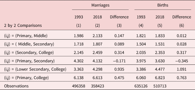
Notes: Vital Statistics Marriage and Birth Records. Men and women are divided into four mutually exclusive education categories: 1. Primary or Less, 2. Middle, 3. Secondary, 4. College. Each row provides the assortative matching measure for the diagonal 2 × 2 sub-matrices of the full sorting matrix using the SEV index.
We preform several robustness checks to examine the sensitivity of the results. First, one concern regarding the use of administrative records of new births and marriages is that we may measure the match prior to one or both of the individuals completing their education. That is, one may get married in one year, and complete more schooling subsequently. To determine the extent to which this is a concern, we limit the sample to individuals age 25 to 54, who are more likely to have completed their education. We present these results in Fig. A5 in the Appendix. The levels are unsurprisingly somewhat different, as age of marriage is likely correlated with education. Nonetheless, the trends over time (which is what we are primarily interested in), are consistent with the results in our main analysis.
A second concern is that our use of administrative marriage records ignores divorce. If non-homogamous marriages are more likely to end in divorce, our use of administrative records for assortative matching may understate the degree of assortative matching in the population.
As a result of these limitations, we complement our main results by computing assortativeness using more standard IPUMS census data. Census data is unable to capture immediate changes in the marriage market, but it does offer us the ability to focus on individuals who's marital status is settled and who have completed their education. In the analysis, we use the 10 percent sample for the years 1970, 1990, 1995, 2000, 2010, and 2015. We compute the SEV index separately for different age groups, as combining adults of all ages would result in comparing very different cohorts together in a given year. That is, most new marriages involve couples who are young so comparing them to the marriage patterns of older adults is not as informative. The results are presented in Fig. A6 and are mostly consistent with our main results in the paper. We see similar levels of the SEV index for all education pairs, as well as similar trends over time. The results are most similar for the younger age groups (15-24 and 25-34) which are likely more comparable to the population we examine with the administrative records.
4.3. Parental matching
In addition to measuring assortativeness among married couples, we also examine parental matching using administrative birth records. As discussed in Sec. 3, there are differential trends in birth and marriage rates across education levels. There may then be differential trends in non-marital childbearing across education levels as well. Moreover, given that intergenerational mobility is a primary reason we study assortative matching, focusing on parental matching is, by itself, relevant.Footnote 25 We repeat our analysis in Sec. 4.2 using the universe of first births in Mexico.Footnote 26
First, Panels A.2 and B.2 of Fig. 3 and Columns 4 to 6 of Table II show that the overall trend in assortativeness across both adjacent and non-adjacent education categories is similar to what we observed using the marriage records. Moreover, the level of assortativeness is also largely similar whether or not we focus on marital or parental matching. Second, an advantage of the birth certificate records is the presence of both unmarried and married couples in the data. Observing marital status allows us to determine if we observe differential patterns in assortativeness across married and unmarried parents. The left half of Fig. 4 and Table III show that the level of assortativeness is mostly higher (five of the six comparisons) among married parents, but there is no systematic difference in trends over time. Why might assortativeness differ across married and unmarried parents? It's possible that marriage rates are simply higher when examining same-educated parents relative to parents with different education levels. Though, a definitive reason is difficult to determine without more information on the couples.
Assortative Parental Matching (Married vs. Non-Married), (A.1) Married: Adjacent Categories, (A.2) Unmarried: Adjacent Categories, (B.1) Married: Non-Adjacent Categories, (B.2) Unmarried: Non-Adjacent Categories. Notes: Vital Statistics Birth Records. Men and women are divided into four mutually exclusive education categories: 1. Primary or Less, 2. Middle, 3. Secondary, 4. College. In Panels A and B, each figure plots assortative matching for the diagonal 2 × 2 sub-matrices of the full sorting matrix using the SEV index. We plot married parents on the left, and unmarried (single and cohabiting) parents on the right. Panel A plots adjacent education categories while Panel B plots non-adjacent categories. The weighted average curve is computed by averaging the assortative index across educational levels, where the weights are determined by diagonal value of the matching table given in Table A3.

Changes in assortativeness 1993–2018 (married vs. non-married)
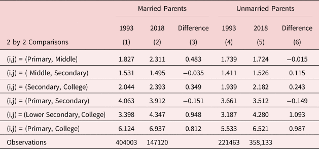
Notes: Vital statistics birth records. Men and women are divided into four mutually exclusive education categories: 1. Primary or Less, 2. Middle, 3. Secondary, 4. College. Each row provides the assortative matching measure for the diagonal 2 × 2 sub-matrices of the full sorting matrix using the SEV index.
4.4. Understanding magnitudes of the SEV index
To better understand how to interpret the magnitudes of the SEV Index, we provide numerical examples of different sorting patterns, and compute what the resulting SEV index is for each of those cases. We limit our attention to two education categories (e.g., college and high school) for simplicity, and use the 2 × 2 measures of assortativeness. To illustrate how to interpret the index, we fix values of m and n, which denote the share of men and women with a college degree as a percentage of men and women with either a college or high school degree, respectively. We then vary r, which measures the share of marriages where both spouses have a college degree. As r increases, there is more assortativeness.
Suppose that we observe 100 married couples. Further, suppose that 40 men have a college degree (m = 0.40), 40 women have a college degree (n = 0.40), and that all other individuals have a high school education. Thus, there can be anywhere from 0 to 40 marriages where both spouses have a college degree. If the 40 college-educated men match with the 40 college-educated women, then the share of college-college matches is r = 0.40, and there is perfect assortative matching (i.e., I SEV = ∞). If there are 16 college-college matches out of 100 (r = mn = 0.16), then there is random matching, and I SEV = 0. If there are no college-college matches, then there is perfect negative assortative matching and I SEV = −∞.
Table A4 further illustrates how the SEV index changes as the rate of homogamous marriages increases. Consistent with the above setup, we fix m and n, and vary r. We see that increasing the share of homogamous marriages does not result in a linear increase in the SEV index. For example, increasing the share of college-college matches from 24 to 28 results in a smaller change (1.42 → 2.23) in the SEV index compared to going from 28 to 32 (2.23 → 3.26).
To relate these hypothetical values to the actual results, it is useful to note that the highest magnitude for the SEV index that we observe is approximately 6.8, where the comparisons are between college graduates and those with only a primary education in 2017. Assuming that m = 0.4 and n = 0.40, that would require that r ≈ 0.38, so that with 100 married couples, 38 would be college educated men matching with college educated women, and there would be four instances of a college educated man or woman matching with a primary educated partner. The lowest magnitude that we observe is roughly 1.5, where the comparisons are between those with a middle or secondary education in 1993. If m and n were to both equal 0.40, then that would imply that out of 100 couples, around 25 would be homogamous matches.
An important limitation of the above discussion of SEV magnitudes is that we fix men's and women's education levels (i.e., m and n). Since m and n change over time, the way in which homogamy rates r translate to the SEV index also changes. This is precisely why homogamy rates are an inadequate measure of assortativeness, but we ignore this fact here in order to provide a rough sense of the relationship between homogamy rates and the SEV index.
4.5. Discussion
To this point, we've established three main results: 1.) assortative matching is highest in non-adjacent education categories, 2.) over time, assortativeness has increased the most among college graduates, and 3.) the patterns in assortativeness do not depend on whether we use marriage records or birth records. We now discuss potential explanations for these findings and their implications.
There are several potential factors that explain the increase in educational assortativeness. First, there may have been reductions in the search costs to finding a spouse due to increased female labor force participation. If women, particularly highly-educated women, are entering the labor market, there are less search frictions in terms of finding a similarly-educated spouse. Given that female labor force participation has grown over the past three decades [Gasparini and Marchionni (Reference Gasparini and Marchionni2017)], it is not surprising that assortativeness has increased. This mechanism is consistent with recent work by Mansour and McKinnish (Reference Mansour and McKinnish2018), who demonstrate that individuals in the United States who share the same occupation prefer a spouse with the same occupation.Footnote 27 More generally, the growing acceptance of women entering the labor force and obtaining a college degree may have shifted norms, resulting in educated men placing greater value in having an educated partner. This mechanism is discussed by Goldin and Katz (Reference Goldin and Katz2002), who examine how family formation for college educated women was affected by the introduction of the pill. Second, recent work suggests that marriage market segmentation reinforces assortative preferences [Jaffe and Weber (Reference Jaffe and Weber2019); Ciscato (Reference Ciscato2021)]. Thus, if more women enter college and the labor force, this may increase the segmentation of the marriage market by education.
Third, changes in legislation governing the marriage market may have also resulted in an increase in assortativeness. Over the past 30 years, Mexico has liberalized its divorce laws, and unilateral divorce is now legal in all 32 states. Recent work by Hoehn-Velasco and Penglase (Reference Hoehn-Velasco and Penglase2021) has found that these laws resulted in a large increase in divorce rates, which suggests that the marriage market was affected more generally. If divorce is easier, this lowers the gains to specializing in home production, since leaving the labor market may have a negative effect on future income, should a divorce occur. Given that this type of specialization is likely most common in negative-assortative marriages, we may expect assortativeness to increase due to liberalized divorce laws.Footnote 28 This mechanism is explored in Liu (Reference Liu2018), who finds that the introduction of unilateral divorce in the United States increased the correlation in both income and education between spouses. A similar pattern may be present in Mexico.
Fourth, Fernández et al. (Reference Fernández, Guner and Knowles2005) and Chiappori et al. (Reference Chiappori, Salanié and Weiss2017) suggest that increases in the returns to education (or skill premium) incentivize highly educated individuals to match with one another, as parental education is an input in child human capital production. Given that the returns to education have risen in Mexico [López-Acevedo (Reference López-Acevedo2004)], this mechanism may apply to our context as well.
Fifth, changes in gender-specific migration patterns may have contributed to the growth in assortativeness. Men in Mexico are much more likely to migrate than women. Migration affects both the marriage outcomes of the migrant, but also the matching patterns of the “sending” community. Choi and Mare (Reference Choi and Mare2012) find evidence that return migrants are more likely to marry outside their education category, and attribute this change to increased income. Moreover, Choi and Mare (Reference Choi and Mare2012) find that in communities where migration is common, there is less assortative matching. It is therefore plausible that the decline in Mexico–U.S. migration over the past decade explains some of the increase in assortativeness.
Finally, an important caveat to our results is that we are restricting the degree of unobserved heterogeneity in preferences to be constant over time. Thus, it may not be the case that preferences for similarly educated partners has increased, but instead preferences for other unobserved factors correlated with education have changed. More general frameworks, such as those employed by Ciscato et al. (Reference Ciscato, Galichon and Goussé2020) or Ciscato and Weber (Reference Ciscato and Weber2020), are necessary to determine the extent to which this is the case.
Regarding the data used in our analysis, our results are largely independent of whether we use administrative records of newly formed marriages, or birth records; Looking at Table II, the signs of the differences in Panel A are constant across columns (3) and (6). One reason for this, is that the assortativeness of married parents is largely similar to that of unmarried parents (see Table III). Given the prevalence of cohabitation, the importance of marriage on fertility behavior may be minimal compared to other contexts. However, an important caveat to the similar results is that they occur when we use first births to measure parental matching. As shown in Fig. A11 and Table A9, the results slightly differ when looking at non-first births. This suggests that there are minimal differences in the probability of having children, conditional on matching, but the number of children a couple has depends on the characteristics of the couple.
5. Conclusion
We study educational assortative matching in Mexico. Understanding who marries whom is essential for uncovering the causes of inequality across households. If both high and low-educated individuals only match within the same education category, the marriage market has the potential to increase income inequality. Moreover, since education is highly correlated across generations, positive assortative matching may exacerbate inequality across time.
Using administrative records on marriages and births, we quantify changes in assortative matching over the past three decades. We focus both on marriage matching, as well as parental matching. This distinction is especially important in a country like Mexico, where not every couple formally marries. To measure assortativeness, we rely on recent work by Chiappori et al. (Reference Chiappori, Salanié, Weiss, Dias and Meghir2020) who demonstrate how one can identify changes in assortativeness over time in such a way that accounts for mechanical increases in homogamous marriages due to converging distributions of male and female education.
Our findings suggest three main patterns. First, we find a moderate increase in average assortativeness across the three decades considered. Moreover, the increase is greatest among college graduates. Second, the level of assortativeness is considerably higher when focusing on non-adjacent versus adjacent education categories; individuals who marry outside their education category are most likely to do so with someone with a similar education level. This suggests that the incidence of college-educated individuals marrying those with less than a high school degree has declined, but this change in assortativeness does not hold when looking at the frequency of college graduates marrying those with a high school degree. Finally, we find that the overall patterns are consistent whether we use data on newly formed marriages, or from birth records. Our results have implications for understanding between-household inequality and child human capital development.
Future work can incorporate singlehood into the analysis. Because we employ birth and marriage records, we do not observe those who are not getting married, or having children. This does not impact the measures of assortativeness [Chiappori et al. (Reference Chiappori, Salanié, Weiss, Dias and Meghir2020)], but it does limit our ability to measure how marital surplus has evolved over time. Moreover, our analysis suggests potential drivers of changes in assortativeness. Further research into several of the potential causes would add to our understanding of marriage market dynamics in Mexico.
Supplementary material
The supplementary material for this article can be found at https://doi.org/10.1017/dem.2022.27
Acknowledgments
We thank Matthew Braaksma, David Lam, David Ribar, and two anonymous referees for helpful comments. We also thank conference participants at the Population Association of America annual meeting. All errors are our own.
Conflict of interest
The authors declare none.


 Open access