


1. Introduction
The Epoch of reionization (EoR) when the diffuse neutral hydrogen (Hi) in the inter-galactic medium (IGM) underwent a transition to the ionised state is one of the least understood phases in the evolution of our Universe. The redshifted 21-cm radiation from Hi is a promising observational probe of EoR (Madau et al. Reference Madau, Meiksin and Rees1997; Bharadwaj & Ali Reference Bharadwaj and Ali2005; McQuinn et al. Reference McQuinn, Zahn, Zaldarriaga, Hernquist and Furlanetto2006; Morales & Wyithe Reference Morales and Wyithe2010; Pritchard & Loeb Reference Pritchard and Loeb2012). Several radio interferometers, such as the Murchison Widefield Array (MWA; Tingay et al. Reference Tingay2013), LOw Frequency ARray (LOFAR; van Haarlem et al. Reference van Haarlem2013), Hydrogen Epoch of Reionization Array (HERA; DeBoer et al. Reference DeBoer2017), Giant Metrewave Radio Telescope (GMRT; Swarup et al. Reference Swarup1991; Gupta et al. Reference Gupta2017) and the upcoming SKA-low (Mellema et al. Reference Mellema2013; Koopmans et al. Reference Koopmans2015) aim to detect the power spectrum (PS) of the EoR 21-cm brightness temperature fluctuations. Despite substantial observational efforts, it has not been possible to detect the EoR 21-cm PS to date, and we only have upper limits (Paciga et al. Reference Paciga2013; Kolopanis et al. Reference Kolopanis2019; Mertens et al. Reference Mertens2020; Trott et al. Reference Trott2020; Pal et al. Reference Pal, Bharadwaj, Ghosh and Choudhuri2021; Abdurashidova et al. Reference Abdurashidova2022; Kolopanis et al. Reference Kolopanis, Pober, Jacobs and McGraw2023). At present we have the best upper limit of $\Delta^2(k) \lt (30.76)^{2} \, \mathrm{mK}^2$
at
$\Delta^2(k) \lt (30.76)^{2} \, \mathrm{mK}^2$
at $k = 0.192\, h\, \mathrm{Mpc}^{-1}$
for
$k = 0.192\, h\, \mathrm{Mpc}^{-1}$
for $z = 7.9$
from HERA (Abdurashidova et al. Reference Abdurashidova2022).
$z = 7.9$
from HERA (Abdurashidova et al. Reference Abdurashidova2022).
The main challenge is that the faint Hi 21-cm signal is buried in foregrounds which are observed to be three to four orders of magnitude brighter (Ali et al. Reference Ali, Bharadwaj and Chengalur2008; Bernardi et al. Reference Bernardi2009; Ghosh et al. Reference Ghosh, Prasad, Bharadwaj, Ali and Chengalur2012; Paciga et al. Reference Paciga2013; Patil et al. Reference Patil2017). In recent years, there have been significant developments to mitigate the foregrounds, relying upon the fact that foregrounds are spectrally smooth compared to the 21-cm signal. Two approaches are generally taken to deal with the foregrounds. In the ‘foreground removal’ approach, one tries to entirely remove the foregrounds (e.g. Chapman et al. Reference Chapman2012; Mertens et al. Reference Mertens, Ghosh and Koopmans2018; Elahi et al. Reference Elahi2023b). An alternative approach, ‘foreground avoidance’, only uses the $(k_\perp, k_{\parallel})$
region outside the ‘foreground wedge’ (Datta et al. Reference Datta, Bowman and Carilli2010; Morales et al. Reference Morales, Hazelton, Sullivan and Beardsley2012; Vedantham et al. Reference Vedantham, Udaya Shankar and Subrahmanyan2012; Trott et al. Reference Trott, Wayth and Tingay2012; Pober et al. Reference Pober2016) to estimate
$(k_\perp, k_{\parallel})$
region outside the ‘foreground wedge’ (Datta et al. Reference Datta, Bowman and Carilli2010; Morales et al. Reference Morales, Hazelton, Sullivan and Beardsley2012; Vedantham et al. Reference Vedantham, Udaya Shankar and Subrahmanyan2012; Trott et al. Reference Trott, Wayth and Tingay2012; Pober et al. Reference Pober2016) to estimate $P(k)$
the spherical PS of the EoR 21-cm signal (e.g. Dillon et al. Reference Dillon2014; Dillon Reference Dillon2015; Trott et al. Reference Trott2020; Pal et al. Reference Pal, Bharadwaj, Ghosh and Choudhuri2021; Abdurashidova et al. Reference Abdurashidova2022).
$P(k)$
the spherical PS of the EoR 21-cm signal (e.g. Dillon et al. Reference Dillon2014; Dillon Reference Dillon2015; Trott et al. Reference Trott2020; Pal et al. Reference Pal, Bharadwaj, Ghosh and Choudhuri2021; Abdurashidova et al. Reference Abdurashidova2022).
The Tapered Gridded Estimator (TGE; Choudhuri et al. Reference Choudhuri, Bharadwaj, Ghosh and Ali2014, Reference Choudhuri2016) is a visibility-based 21-cm PS estimator that has been extensively used for measuring the 21-cm PS (Pal et al. Reference Pal, Bharadwaj, Ghosh and Choudhuri2021, Reference Pal2022; Elahi et al. Reference Elahi2023a,Reference Elahib, Reference Elahi2024) and for characterising the diffused Galactic foregrounds Choudhuri et al. (Reference Choudhuri2017) and magnetohydrodynamic turbulence (Saha et al. Reference Saha, Bharadwaj, Roy, Choudhuri and Chattopadhyay2019, Reference Saha2021). The main attribute of TGE is that it suppresses the sidelobe responses of the telescope to mitigate the effects of extra-galactic point source foregrounds (Ghosh et al. Reference Ghosh, Bharadwaj, Ali and Chengalur2011a,b). Additionally, the TGE is computationally efficient as it deals with gridded visibilities. It is also an unbiased estimator as it internally estimates the noise bias from the self-correlation of the visibilities to yield an unbiased estimate of the PS. In a recent work Chatterjee et al. (Reference Chatterjee, Bharadwaj, Choudhuri, Sethi and Patwa2022) (hereafter, Reference Chatterjee, Bharadwaj, Choudhuri, Sethi and PatwaPaper I) have introduced the Tracking Tapered Gridded Estimator (TTGE), which generalises the TGE for estimating the 21-cm PS from drift scan observations. Reference Chatterjee, Bharadwaj, Choudhuri, Sethi and PatwaPaper I has also validated the TTGE considering simulated MWA drift scan observations at a single frequency, where it was demonstrated that the estimated $C_{\ell}$
matches the input model
$C_{\ell}$
matches the input model $C^M_{\ell}$
.
$C^M_{\ell}$
.
Missing frequency channels, flagged to remove radio frequency interferences (RFIs) or for other reasons, pose a serious problem for visibility-based PS estimation. The Fourier transform from frequency to delay space (e.g. Morales & Hewitt Reference Morales and Hewitt2004; Parsons & Backer Reference Parsons and Backer2009) introduces artefacts in the estimated PS, and there has been substantial work to address this problem (Parsons & Backer Reference Parsons and Backer2009; Parsons et al. Reference Parsons2014; Trott Reference Trott2016; Kern & Liu Reference Kern and Liu2021; Ewall-Wice et al. Reference Ewall-Wice2021; Kennedy et al. Reference Kennedy, Bull, Wilensky, Burba and Choudhuri2023). We, however, note that this problem does not arise if we correlate the visibilities directly in the frequency domain (Bharadwaj & Sethi Reference Bharadwaj and Sethi2001; Bharadwaj & Ali Reference Bharadwaj and Ali2005) and use this to estimate the 21-cm signal. The TGE and the TTGE first correlate the visibilities to estimate $C_{\ell}(\Delta\nu)$
the multi-frequency angular power spectrum (MAPS; Datta et al. Reference Datta, Choudhury and Bharadwaj2007; Mondal et al. Reference Mondal, Bharadwaj and Datta2018) and then Fourier transforms
$C_{\ell}(\Delta\nu)$
the multi-frequency angular power spectrum (MAPS; Datta et al. Reference Datta, Choudhury and Bharadwaj2007; Mondal et al. Reference Mondal, Bharadwaj and Datta2018) and then Fourier transforms $C_{\ell}(\Delta\nu)$
along the
$C_{\ell}(\Delta\nu)$
along the $\Delta\nu$
to estimate
$\Delta\nu$
to estimate $P(k_\perp, k_{\parallel})$
the cylindrical PS. Using simulations Bharadwaj et al. (Reference Bharadwaj, Pal, Choudhuri and Dutta2018) have shown that
$P(k_\perp, k_{\parallel})$
the cylindrical PS. Using simulations Bharadwaj et al. (Reference Bharadwaj, Pal, Choudhuri and Dutta2018) have shown that $C_{\ell}(\Delta\nu)$
does not exhibit any missing
$C_{\ell}(\Delta\nu)$
does not exhibit any missing $\Delta\nu$
values even when
$\Delta\nu$
values even when $80 \%$
of randomly chosen frequency channels are flagged in the visibility data, and it is possible to estimate
$80 \%$
of randomly chosen frequency channels are flagged in the visibility data, and it is possible to estimate $P(k_\perp, k_{\parallel})$
without any artefacts due to the missing channels. This has been further borne out in the analysis of actual data using the TGE (Pal et al. Reference Pal, Bharadwaj, Ghosh and Choudhuri2021, Reference Pal2022; Elahi et al. Reference Elahi2023a,Reference Elahib, Reference Elahi2024).
$P(k_\perp, k_{\parallel})$
without any artefacts due to the missing channels. This has been further borne out in the analysis of actual data using the TGE (Pal et al. Reference Pal, Bharadwaj, Ghosh and Choudhuri2021, Reference Pal2022; Elahi et al. Reference Elahi2023a,Reference Elahib, Reference Elahi2024).
MWA has a periodic pattern of flagged channels in the visibility data, which introduce horizontal streaks in $P(k_\perp, k_{\parallel})$
(Paul et al. Reference Paul2016; Li et al. Reference Li2019; Trott et al. Reference Trott2020; Patwa et al. Reference Patwa, Sethi and Dwarakanath2021). In this paper, we consider the MWA drift scan observation used in Patwa et al. (Reference Patwa, Sethi and Dwarakanath2021). Here we investigate if the TTGE can overcome this issue. For this, we first simulated the MWA drift scan observation with exactly the same flagging as in the actual data and used this to verify if the TTGE can faithfully recover the input model PS used for the simulations. We have subsequently applied the TTGE to actual observations and present preliminary results here.
$P(k_\perp, k_{\parallel})$
(Paul et al. Reference Paul2016; Li et al. Reference Li2019; Trott et al. Reference Trott2020; Patwa et al. Reference Patwa, Sethi and Dwarakanath2021). In this paper, we consider the MWA drift scan observation used in Patwa et al. (Reference Patwa, Sethi and Dwarakanath2021). Here we investigate if the TTGE can overcome this issue. For this, we first simulated the MWA drift scan observation with exactly the same flagging as in the actual data and used this to verify if the TTGE can faithfully recover the input model PS used for the simulations. We have subsequently applied the TTGE to actual observations and present preliminary results here.
We have arranged the paper in the following manner. First, we describe the MWA drift scan observation in Section 2. In Section 3, we present the TTGE and the formalism for the PS. Section 4 describes the simulations and the validation of the TTGE. We have shown the preliminary results from actual MWA observation in Section 5. We summarise and discuss our findings in Section 6.
2. MWA drift-scan observation
The data analysed here is from Phase II (compact configuration) of the MWA (Lonsdale et al. Reference Lonsdale2009; Wayth et al. Reference Wayth2018) which is a radio interferometer with 128 tiles (antennas in rest of the paper) located in Western Australia (latitude $-26.7^\circ$
, longitude
$-26.7^\circ$
, longitude $116.7^\circ$
). Each antenna consists of 16 crossed dipoles placed in a
$116.7^\circ$
). Each antenna consists of 16 crossed dipoles placed in a $4\times 4$
arrangement on a square mesh of side
$4\times 4$
arrangement on a square mesh of side $\sim$ $4 \, \mathrm{m}$
. MWA operates in several frequency bands ranging from 80 to 300 MHz. The observed visibilities are recorded with the time resolution of 0.5 s, and they are written out at an interval of 2 min (one snapshot) in which the actual duration of observation is 112 s.
$4 \, \mathrm{m}$
. MWA operates in several frequency bands ranging from 80 to 300 MHz. The observed visibilities are recorded with the time resolution of 0.5 s, and they are written out at an interval of 2 min (one snapshot) in which the actual duration of observation is 112 s.
For this work we consider a particular drift scan observation (project ID G0031) that is described in Patwa et al. (Reference Patwa, Sethi and Dwarakanath2021). In short, the observation is at a fixed declination (DEC) $-26.7^{\circ}$
which corresponds to the zenith and it covers a region of the sky from right ascension (RA)
$-26.7^{\circ}$
which corresponds to the zenith and it covers a region of the sky from right ascension (RA) $349^{\circ}$
to
$349^{\circ}$
to $70.3^{\circ}$
which spans
$70.3^{\circ}$
which spans $81.3^{\circ}$
in RA over a time duration of 5 hr 24 min. The beginning and end of the drift scan observation are marked with
$81.3^{\circ}$
in RA over a time duration of 5 hr 24 min. The beginning and end of the drift scan observation are marked with $\star$
in Fig. 1. Visibilities are recorded every 2 min which leads to 162 different pointing centres (PCs, labelled PC=1,2,…,162), located at an interval of
$\star$
in Fig. 1. Visibilities are recorded every 2 min which leads to 162 different pointing centres (PCs, labelled PC=1,2,…,162), located at an interval of $0.5^{\circ}$
along RA. This region includes two well observed MWA fields namely EoR 0 (
$0.5^{\circ}$
along RA. This region includes two well observed MWA fields namely EoR 0 ( $0^{\circ}, -26.7^{\circ}$
) and EoR 1 (
$0^{\circ}, -26.7^{\circ}$
) and EoR 1 ( $60^{\circ}, -26.7^{\circ}$
) which are also shown in Fig. 1. The same drift scan observation was carried out on 10 consecutive nights. The present observation has been performed at a nominal frequency of
$60^{\circ}, -26.7^{\circ}$
) which are also shown in Fig. 1. The same drift scan observation was carried out on 10 consecutive nights. The present observation has been performed at a nominal frequency of $\nu_c=154.2 \, \mathrm{MHz}$
(nominal redshift
$\nu_c=154.2 \, \mathrm{MHz}$
(nominal redshift $z_c=8.2$
) with
$z_c=8.2$
) with $N_c = 768$
channels of resolution of
$N_c = 768$
channels of resolution of $\Delta\nu_c=40 \, \mathrm{kHz}$
covering the observing bandwidth of
$\Delta\nu_c=40 \, \mathrm{kHz}$
covering the observing bandwidth of $B_\mathrm{bw} = 30.72$
MHz. This is further divided into 24 coarse bands each containing 32 channels or
$B_\mathrm{bw} = 30.72$
MHz. This is further divided into 24 coarse bands each containing 32 channels or $1.28 \, \mathrm{MHz}$
.
$1.28 \, \mathrm{MHz}$
.
This shows the $408 \, \mathrm{MHz}$
Haslam map (Haslam et al. Reference Haslam, Salter, Stoffel and Wilson1982) scaled to 154 MHz assuming the brightness temperature spectral index
$408 \, \mathrm{MHz}$
Haslam map (Haslam et al. Reference Haslam, Salter, Stoffel and Wilson1982) scaled to 154 MHz assuming the brightness temperature spectral index $\alpha = -2.52$
(Rogers & Bowman Reference Rogers and Bowman2008). The iso-contours in green, magenta, red, and black show the MWA primary beam at values 0.9, 0.5, 0.05, and 0.005, respectively, for a pointing centre at (
$\alpha = -2.52$
(Rogers & Bowman Reference Rogers and Bowman2008). The iso-contours in green, magenta, red, and black show the MWA primary beam at values 0.9, 0.5, 0.05, and 0.005, respectively, for a pointing centre at ( $6.1^{\circ}, -26.7^{\circ}$
) which corresponds to the data analysed here. The scan starts roughly at the location of the ‘
$6.1^{\circ}, -26.7^{\circ}$
) which corresponds to the data analysed here. The scan starts roughly at the location of the ‘ $\star$
’ on the right (RA=
$\star$
’ on the right (RA= $349^{\circ}$
) and lasts until the ‘
$349^{\circ}$
) and lasts until the ‘ $\star$
’ on the left (RA=
$\star$
’ on the left (RA= $70.3^{\circ}$
). Blue filled circles mark the fields EoR 0(
$70.3^{\circ}$
). Blue filled circles mark the fields EoR 0( $0^{\circ}, -26.7^{\circ}$
) and EoR 1(
$0^{\circ}, -26.7^{\circ}$
) and EoR 1( $60^{\circ}, -26.7^{\circ}$
). The red circle shows the position of Fornax A.
$60^{\circ}, -26.7^{\circ}$
). The red circle shows the position of Fornax A.

The data has been pre-processed with COTTER (Offringa et al. Reference Offringa2015) which flags RFI and non-working antennas. For each coarse band, COTTER also flags four channels at both ends and one channel at the centre resulting in channels (1-4,17,29-32) to be flagged. The produces a period pattern of flagged channels as shown in Fig. 2. We apply COTTER individually to the 0.5 s time resolution visibility data and then average them to 10 s time resolution. This pre-processed data is written in CASA
Footnote
a
readable Measurement Sets (MS). The MS for 10 nights are calibrated separately using the steps mentioned in Patwa et al. (Reference Patwa, Sethi and Dwarakanath2021). We note that the first $2 \, \mathrm{hr}$
of data is missing from the 6-th night, and as a consequence the nights of observations is
$2 \, \mathrm{hr}$
of data is missing from the 6-th night, and as a consequence the nights of observations is $N_\mathrm{nights}=10$
for some PCs whereas it is
$N_\mathrm{nights}=10$
for some PCs whereas it is $N_\mathrm{nights}=9$
for others. Since the observations covers the same region of the sky, we perform Local Sidereal Time (LST) stacking (e.g. Bandura et al. Reference Bandura2014; CHIME Collaboration et al. 2022) and obtain the equivalent one night drift scan data. We finally have 162 MS, each corresponding to a different pointing direction on the sky. Each MS contains visibility data with 11 different time stamps each with
$N_\mathrm{nights}=9$
for others. Since the observations covers the same region of the sky, we perform Local Sidereal Time (LST) stacking (e.g. Bandura et al. Reference Bandura2014; CHIME Collaboration et al. 2022) and obtain the equivalent one night drift scan data. We finally have 162 MS, each corresponding to a different pointing direction on the sky. Each MS contains visibility data with 11 different time stamps each with $t_\mathrm{int}= N_\mathrm{nights} \times 10 \, \mathrm{s}$
effective integration time.
$t_\mathrm{int}= N_\mathrm{nights} \times 10 \, \mathrm{s}$
effective integration time.
This shows the periodic channel flagging in the observed MWA visibility data. The entire frequency bandwidth is divided into 24 coarse bands of 32 channels or $1.28 \, \mathrm{MHz}$
width each. The colours here shows arbitrarily normalised visibility amplitudes, and the black vertical lines indicate the flagged channels.
$1.28 \, \mathrm{MHz}$
width each. The colours here shows arbitrarily normalised visibility amplitudes, and the black vertical lines indicate the flagged channels.

In addition to the sky signal, each measured visibility also has a system noise contribution. For the present data, $\unicode{x03C3}_\mathrm{N}$
the r.m.s. system noise for the real (and also imaginary) part of the measured visibilities is estimated using
$\unicode{x03C3}_\mathrm{N}$
the r.m.s. system noise for the real (and also imaginary) part of the measured visibilities is estimated using
 \begin{eqnarray} \unicode{x03C3}_\mathrm{N} = \frac{1}{\unicode{x03B7}_s} \frac{2 K_\mathrm{B} T_\mathrm{sys} }{A_\mathrm{eff} \sqrt{\Delta\nu t_\mathrm{int}}} \end{eqnarray}
where the $A_\mathrm{eff} = 21.4 \, \mathrm{m}^2$
and
$A_\mathrm{eff} = 21.4 \, \mathrm{m}^2$
and $T_\mathrm{sys} / \unicode{x03B7}_s = 290\,\mathrm{K}$
(Patwa et al. Reference Patwa, Sethi and Dwarakanath2021). This yields
$T_\mathrm{sys} / \unicode{x03B7}_s = 290\,\mathrm{K}$
(Patwa et al. Reference Patwa, Sethi and Dwarakanath2021). This yields $\unicode{x03C3}_\mathrm{N} = [N_\mathrm{nights}]^{-0.5} \times 60 \, \mathrm{Jy}$
for a single visibility.
$\unicode{x03C3}_\mathrm{N} = [N_\mathrm{nights}]^{-0.5} \times 60 \, \mathrm{Jy}$
for a single visibility.
Considering the baseline distribution, 99 per cent of the baselines are found to be smaller than 500 m, that is, $257.8\unicode{x03BB}$
(Figure 2 of Reference Chatterjee, Bharadwaj, Choudhuri, Sethi and PatwaPaper I), and we have restricted the baseline range in our analysis to
$257.8\unicode{x03BB}$
(Figure 2 of Reference Chatterjee, Bharadwaj, Choudhuri, Sethi and PatwaPaper I), and we have restricted the baseline range in our analysis to $\mid U \mid \leq 245 \unicode{x03BB}$
.
$\mid U \mid \leq 245 \unicode{x03BB}$
.
3. The tracking TGE $T(\hat{\textbf{n}}, \nu)$
the brightness temperature distribution on the sky is decomposed into spherical harmonics
$T(\hat{\textbf{n}}, \nu)$
the brightness temperature distribution on the sky is decomposed into spherical harmonics $Y_{\ell}^{m}(\hat{\textbf{n}})$
using
$Y_{\ell}^{m}(\hat{\textbf{n}})$
using
 \begin{equation} T(\hat{\textbf{n}}, \nu) = \sum_{\ell, m}a_{\ell}^{m}(\nu) Y_{\ell}^{m}(\hat{\textbf{n}}) \end{equation}
where $a_{\ell}^{m}(\nu)$
are the expansion coefficients. The MAPS which is defined as
$a_{\ell}^{m}(\nu)$
are the expansion coefficients. The MAPS which is defined as
 \begin{equation} C_{\ell}(\nu_a,\nu_b) = \langle a_{\ell}^{m}(\nu_a) a_{\ell}^{m *}(\nu_b) \rangle \,, \end{equation}
jointly characterises the angular and frequency dependence of the two-point statistics of $T(\hat{\textbf{n}}, \nu)$
. Further, the MAPS is a function of the frequency separation
$T(\hat{\textbf{n}}, \nu)$
. Further, the MAPS is a function of the frequency separation
 \begin{equation} C_{\ell}(\nu_a, \nu_b) = C_{\ell}(\Delta\nu) \,\, \mathrm{where} \,\, \Delta \nu= \mid \nu_b-\nu_a\mid \end{equation}
if $T(\hat{\textbf{n}}, \nu)$
is assumed to be statistically homogeneous (ergodic) along the line of sight direction.
$T(\hat{\textbf{n}}, \nu)$
is assumed to be statistically homogeneous (ergodic) along the line of sight direction.
Reference Chatterjee, Bharadwaj, Choudhuri, Sethi and PatwaPaper I presents the TTGE to determine the MAPS $C_{\ell}(\nu_a,\nu_b)$
using the measured visibility data from drift scan radio-interferometric observations. Reference Chatterjee, Bharadwaj, Choudhuri, Sethi and PatwaPaper I also explained how
$C_{\ell}(\nu_a,\nu_b)$
using the measured visibility data from drift scan radio-interferometric observations. Reference Chatterjee, Bharadwaj, Choudhuri, Sethi and PatwaPaper I also explained how $C_{\ell}(\nu_a,\nu_b)$
can be used to determine the cylindrical PS
$C_{\ell}(\nu_a,\nu_b)$
can be used to determine the cylindrical PS $P(k_{\perp},k_{\parallel})$
. However, the validation in that paper is restricted to a single frequency
$P(k_{\perp},k_{\parallel})$
. However, the validation in that paper is restricted to a single frequency $\nu$
. There, we have simulated observations where the sky signal
$\nu$
. There, we have simulated observations where the sky signal $T(\hat{\textbf{n}})$
corresponds to an input model
$T(\hat{\textbf{n}})$
corresponds to an input model $C^M_{\ell}$
. We have applied TTGE on the simulated visibilities to estimate
$C^M_{\ell}$
. We have applied TTGE on the simulated visibilities to estimate $C_{\ell}$
and demonstrated that the estimated
$C_{\ell}$
and demonstrated that the estimated $C_{\ell}$
matches the input model. In this section of the present paper, we briefly summarise the formalism of the TTGE, and in Section 4, we validate it considering multi-frequency observations and the full three-dimensional PS
$C_{\ell}$
matches the input model. In this section of the present paper, we briefly summarise the formalism of the TTGE, and in Section 4, we validate it considering multi-frequency observations and the full three-dimensional PS $P(k)$
.
$P(k)$
.
The visibility $\mathcal{V}\left( \textbf{U}, \nu \right)$
measured at a baseline
$\mathcal{V}\left( \textbf{U}, \nu \right)$
measured at a baseline $\textbf{U}$
and frequency
$\textbf{U}$
and frequency $\nu$
is given by:
$\nu$
is given by:
 \begin{equation}\mathcal{V}\left( \textbf{U}, \nu \right) = Q_{\nu} \int d\Omega_{\hat{\textbf{n}}}T\left(\hat{\textbf{n}},\nu \right) A\left(\Delta \hat{\textbf{n}},\nu\right) e^{2 \pi i \textbf{U}\cdot \Delta \textbf{n} },\end{equation}
where $Q_{\nu} = 2 k_B / \unicode{x03BB}^2$
is the conversion factor from brightness temperature to specific intensity in the Raleigh-Jeans limit,
$Q_{\nu} = 2 k_B / \unicode{x03BB}^2$
is the conversion factor from brightness temperature to specific intensity in the Raleigh-Jeans limit, $T\left(\hat{\textbf{n}},\nu \right)$
is the brightness temperature distribution on the sky,
$T\left(\hat{\textbf{n}},\nu \right)$
is the brightness temperature distribution on the sky, $d\Omega_{\hat{\textbf{n}}}$
is the elemental solid angle in the direction
$d\Omega_{\hat{\textbf{n}}}$
is the elemental solid angle in the direction $\hat{\textbf{n}}$
,
$\hat{\textbf{n}}$
, $A\left(\Delta \hat{\textbf{n}},\nu \right)$
is the antenna primary beam (PB) pattern, and
$A\left(\Delta \hat{\textbf{n}},\nu \right)$
is the antenna primary beam (PB) pattern, and $\Delta \hat{\textbf{n}} =\hat{\textbf{n}} -\hat{\textbf{p}}$
where
$\Delta \hat{\textbf{n}} =\hat{\textbf{n}} -\hat{\textbf{p}}$
where $\hat{\textbf{p}}$
is the telescope’s pointing direction or PC. In this work, we consider drift scan observations where the telescope is held fixed (on earth) to point towards the zenith. Here
$\hat{\textbf{p}}$
is the telescope’s pointing direction or PC. In this work, we consider drift scan observations where the telescope is held fixed (on earth) to point towards the zenith. Here $\hat{\textbf{p}}$
has a fixed declination
$\hat{\textbf{p}}$
has a fixed declination $\unicode{x03B4}_0$
(latitude of the array), whereas the RA
$\unicode{x03B4}_0$
(latitude of the array), whereas the RA $\alpha_p$
varies due to the earth’s rotation. In such a situation, it is convenient to use
$\alpha_p$
varies due to the earth’s rotation. In such a situation, it is convenient to use $\mathcal{V}(\alpha_p,\textbf{U}_i,\nu_a)$
where we have included
$\mathcal{V}(\alpha_p,\textbf{U}_i,\nu_a)$
where we have included $\alpha_p$
as a parameter which tells us the pointing direction
$\alpha_p$
as a parameter which tells us the pointing direction $\hat{\textbf{p}}$
for which the visibilities were recorded. As noted earlier, for the observations considered here, we have
$\hat{\textbf{p}}$
for which the visibilities were recorded. As noted earlier, for the observations considered here, we have $\unicode{x03B4}_0=-26.7^{\circ}$
and
$\unicode{x03B4}_0=-26.7^{\circ}$
and $349^{\circ} \le \alpha_p \le 70.3^{\circ}$
at an interval
$349^{\circ} \le \alpha_p \le 70.3^{\circ}$
at an interval $\Delta \alpha_p =0.5^{\circ}$
.
$\Delta \alpha_p =0.5^{\circ}$
.
The question is ‘How do we combine the visibility data from different $\hat{\textbf{p}}$
?’. To address this, we choose a tracking centre (TC)
$\hat{\textbf{p}}$
?’. To address this, we choose a tracking centre (TC) $\hat{\textbf{c}}$
which remains fixed on the sky and consider the convolved visibilities defined in the uv plane as:
$\hat{\textbf{c}}$
which remains fixed on the sky and consider the convolved visibilities defined in the uv plane as:
 \begin{equation} \mathcal{V}_c(\alpha_p,\textbf{U},\nu)=\int d^2 U^{'} \, \tilde{w}(\textbf{U}-\textbf{U}^{'}) \, e^{2 \pi i \textbf{U}^{'} \cdot \unicode{x1D6D8}_p } \, \mathcal{V}(\alpha_p,\textbf{U}^{'},\nu) \, \end{equation}
where $\unicode{x1D6D8}_p=\hat{\textbf{p}} -\hat{\textbf{c}}$
and
$\unicode{x1D6D8}_p=\hat{\textbf{p}} -\hat{\textbf{c}}$
and $\tilde{w}(\textbf{U})$
is the Fourier transform of a tapering function
$\tilde{w}(\textbf{U})$
is the Fourier transform of a tapering function $W\left(\unicode{x1D6C9} \right)$
which is typically chosen to be considerably narrower than the antenna’s PB pattern
$W\left(\unicode{x1D6C9} \right)$
which is typically chosen to be considerably narrower than the antenna’s PB pattern $A\left(\unicode{x1D6C9},\nu \right)$
. Here we have used a Gaussian
$A\left(\unicode{x1D6C9},\nu \right)$
. Here we have used a Gaussian $ W\left(\unicode{x1D6C9} \right)=e^{-\unicode{x03B8}^2/\unicode{x03B8}_w^2}$
. Adopting the flat-sky approximation, equation (6) can be expressed as
$ W\left(\unicode{x1D6C9} \right)=e^{-\unicode{x03B8}^2/\unicode{x03B8}_w^2}$
. Adopting the flat-sky approximation, equation (6) can be expressed as
 \begin{equation} \mathcal{V}_c(\alpha_p,\textbf{U},\nu)=Q_{\nu} \int d^2 \unicode{x03B8} \,T\left(\unicode{x1D6C9},\nu \right) \, W(\unicode{x1D6C9}) \, A\left(\unicode{x1D6C9}-\unicode{x1D6D8}_p,\nu\right) e^{2 \pi i \textbf{U} \cdot \unicode{x1D6C9} }\end{equation}
where the phase centre of $\mathcal{V}_c(\textbf{U},\nu)$
is shifted to
$\mathcal{V}_c(\textbf{U},\nu)$
is shifted to $\hat{\textbf{c}}$
, and the function
$\hat{\textbf{c}}$
, and the function $W(\unicode{x1D6C9})$
restricts the sky response to a small region around
$W(\unicode{x1D6C9})$
restricts the sky response to a small region around $\hat{\textbf{c}}$
. For the purpose of this discussion, we may assume that the convolved visibility
$\hat{\textbf{c}}$
. For the purpose of this discussion, we may assume that the convolved visibility $\mathcal{V}_c(\alpha_p,\textbf{U},\nu)$
only records the signal from a small region of the sky centred around
$\mathcal{V}_c(\alpha_p,\textbf{U},\nu)$
only records the signal from a small region of the sky centred around $\hat{\textbf{c}}$
. We can now coherently combine the data from different pointings
$\hat{\textbf{c}}$
. We can now coherently combine the data from different pointings
 \begin{equation} \mathcal{V}_c(\textbf{U},\nu)= \sum_p s_p \mathcal{V}_c(\alpha_p,\textbf{U},\nu)\end{equation}
to estimate the sky signal from a small region around $\hat{\textbf{c}}$
. The contribution to
$\hat{\textbf{c}}$
. The contribution to $\mathcal{V}_c(\textbf{U},\nu)$
from
$\mathcal{V}_c(\textbf{U},\nu)$
from $\mathcal{V}_c(\alpha_p,\textbf{U},\nu)$
at a particular PC
$\mathcal{V}_c(\alpha_p,\textbf{U},\nu)$
at a particular PC $\hat{\textbf{p}}$
goes down as
$\hat{\textbf{p}}$
goes down as $\sim A\left(-\unicode{x1D6D8}_p,\nu\right)$
(equation (7)) which declines rapidly as the separation
$\sim A\left(-\unicode{x1D6D8}_p,\nu\right)$
(equation (7)) which declines rapidly as the separation $\unicode{x1D6D8}_p=\hat{\textbf{p}}-\hat{\textbf{c}}$
increases. In addition to the sky signal, each
$\unicode{x1D6D8}_p=\hat{\textbf{p}}-\hat{\textbf{c}}$
increases. In addition to the sky signal, each $\mathcal{V}_c(\alpha_p,\textbf{U},\nu)$
also contains a system noise contribution. This implies that the PC
$\mathcal{V}_c(\alpha_p,\textbf{U},\nu)$
also contains a system noise contribution. This implies that the PC $\hat{\textbf{p}}$
, which are close to
$\hat{\textbf{p}}$
, which are close to $\hat{\textbf{c}}$
contribute to
$\hat{\textbf{c}}$
contribute to $\mathcal{V}_c(\textbf{U},\nu)$
with a relatively high signal-to-noise ratio (SNR) as compared to those which are at a large angular distance from
$\mathcal{V}_c(\textbf{U},\nu)$
with a relatively high signal-to-noise ratio (SNR) as compared to those which are at a large angular distance from $\hat{\textbf{c}}$
. We account for this by suitably choosing the factor
$\hat{\textbf{c}}$
. We account for this by suitably choosing the factor $s_p$
, which assigns different weights to every PC.
$s_p$
, which assigns different weights to every PC.
Considering the observational data, we evaluate the convolved visibilities on a rectangular grid (labelled using g) on a uv plane. Note that our analysis does not account for the fact that the baseline $\textbf{U} = \textbf{d} \nu/c$
corresponding to a fixed antenna separation
$\textbf{U} = \textbf{d} \nu/c$
corresponding to a fixed antenna separation $\textbf{d}$
changes with frequency, and it is held fixed at the value corresponding to
$\textbf{d}$
changes with frequency, and it is held fixed at the value corresponding to $\nu_c$
. The convolved gridded visibilities are evaluated using
$\nu_c$
. The convolved gridded visibilities are evaluated using
 \begin{align} \mathcal{V}_{cg}(\nu_a) = \sum_{p} s_p \sum_{n} & \tilde{w}(\textbf{U}_g-\textbf{U}_i) e^{2 \pi i \textbf{U}_i \cdot \unicode{x1D6D8}_p } \times \nonumber \\ & \mathcal{V}(\alpha_p,\textbf{U}_i,\nu_a) F_{p, n}(\nu_a) \,\end{align}
where $F_{p, n}(\nu_a)$
has a value 0 if the particular visibility is flagged and is 1 otherwise. Here, the sum over different baselines
$F_{p, n}(\nu_a)$
has a value 0 if the particular visibility is flagged and is 1 otherwise. Here, the sum over different baselines $\textbf{U}_i$
is evaluated for a fixed PC (labelled p), whereas the outer sum combines all the different PCs covered in the drift scan observation. The final
$\textbf{U}_i$
is evaluated for a fixed PC (labelled p), whereas the outer sum combines all the different PCs covered in the drift scan observation. The final $\mathcal{V}_{cg}(\nu_a)$
refers to the sky signal centred at a particular TC
$\mathcal{V}_{cg}(\nu_a)$
refers to the sky signal centred at a particular TC $\hat{\textbf{c}}$
.
$\hat{\textbf{c}}$
.
Following equation (6) of Pal et al. (Reference Pal2022), we define the TTGE as:
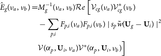 \begin{align} \hat{E}_g(\nu_a,\nu_b) = & M^{-1}_g(\nu_a,\nu_b) {\mathcal Re} \, \Big{[} \mathcal{V}_{cg}(\nu_a) \mathcal{V}^*_{cg}(\nu_b) \nonumber \\ & - \sum_{p,i} F_{p, i}(\nu_a) F_{p, i}(\nu_b) \mid s_p \tilde{w}(\textbf{U}_g-\textbf{U}_i) \mid^2 \nonumber \\ & \mathcal{V}(\alpha_p,\textbf{U}_i,\nu_a) \mathcal{V}^*(\alpha_p,\textbf{U}_i,\nu_b) \Big{]}\end{align}
where $M_g(\nu_a,\nu_b)$
is a normalisation factor and
$M_g(\nu_a,\nu_b)$
is a normalisation factor and ${\mathcal Re}[]$
denotes the real part. The second term in the r.h.s. of equation (10) subtract out the contribution from the correlation between the visibilities measured at the same baseline and pointing direction. This is primarily introduced to cancel out the noise bias which arises when we correlate a visibility with itself (i.e.
${\mathcal Re}[]$
denotes the real part. The second term in the r.h.s. of equation (10) subtract out the contribution from the correlation between the visibilities measured at the same baseline and pointing direction. This is primarily introduced to cancel out the noise bias which arises when we correlate a visibility with itself (i.e. $a=b$
; Reference Chatterjee, Bharadwaj, Choudhuri, Sethi and PatwaPaper I).
$a=b$
; Reference Chatterjee, Bharadwaj, Choudhuri, Sethi and PatwaPaper I).
We use all-sky simulations (Section 4.1) to estimate $M_g(\nu_a,\nu_b)$
. The simulated sky signal
$M_g(\nu_a,\nu_b)$
. The simulated sky signal $T(\hat{\textbf{n}},\nu)$
is a realisation of a Gaussian random field (GRF) corresponding to an unit multi-frequency angular power spectrum (UMAPS) where
$T(\hat{\textbf{n}},\nu)$
is a realisation of a Gaussian random field (GRF) corresponding to an unit multi-frequency angular power spectrum (UMAPS) where $C_{\ell}(\nu_a,\nu_b)=1$
. The simulations consider identical drift scan observations as the actual data, with exactly the same flagging, and frequency and baseline coverage. The simulated visibilities
$C_{\ell}(\nu_a,\nu_b)=1$
. The simulations consider identical drift scan observations as the actual data, with exactly the same flagging, and frequency and baseline coverage. The simulated visibilities $ [\mathcal{V}(\alpha_p,\textbf{U}_i,\nu_a)]_\mathrm{UMAPS}$
are analysed exactly the same as the actual data. We have estimated
$ [\mathcal{V}(\alpha_p,\textbf{U}_i,\nu_a)]_\mathrm{UMAPS}$
are analysed exactly the same as the actual data. We have estimated $M_g(\nu_a,\nu_b)$
using
$M_g(\nu_a,\nu_b)$
using
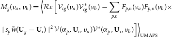 \begin{align} & M_g (\nu_a, \nu_b)= \Big{\langle } {\mathcal Re} \, \Big{[} \mathcal{V}_{cg}(\nu_a) \mathcal{V}^*_{cg}(\nu_b) - \sum_{p,n} F_{p, n}(\nu_a) F_{p, n}(\nu_b) \times \nonumber \\ & \mid s_p \tilde{w}(\textbf{U}_g-\textbf{U}_i) \mid^2 \mathcal{V}(\alpha_p,\textbf{U}_i,\nu_a) \mathcal{V}^*(\alpha_p,\textbf{U}_i,\nu_b) \Big{]} \Big{\rangle}_\mathrm{UMAPS} \end{align}
where the angular brackets $\langle \ldots \rangle$
denote an average over multiple realisations of the UMAPS. Here we have used 100 random realisations of the UMAPS to reduce the statistical uncertainties in the estimated
$\langle \ldots \rangle$
denote an average over multiple realisations of the UMAPS. Here we have used 100 random realisations of the UMAPS to reduce the statistical uncertainties in the estimated $M_g(\nu_a,\nu_b)$
.
$M_g(\nu_a,\nu_b)$
.
The MAPS TTGE defined in equation (10) provides an unbiased estimate of $C_{\ell}{_g}(\nu_a,\nu_b)$
at the angular multipole
$C_{\ell}{_g}(\nu_a,\nu_b)$
at the angular multipole $\ell_g=2 \pi U_g$
, that is,
$\ell_g=2 \pi U_g$
, that is,
 \begin{equation}\langle {\hat E}_g(\nu_a,\nu_b) \rangle = C_{\ell}{_g}(\nu_a,\nu_b)\end{equation}
To enhance the SNR and also reduce the data volume, we have divided the uv plane into annular bins. We use this to define the binned TTGE
 \begin{equation}\hat{E}_G[q](\nu_a,\nu_b) = \frac{\sum_g w_g {\hat E}_g(\nu_a,\nu_b)}{\sum_g w_g } \,.\end{equation}
where $w_g$
refers to the weight assigned to the contribution from any particular grid point
$w_g$
refers to the weight assigned to the contribution from any particular grid point $g$
. For the analysis presented in this paper we have used the weight
$g$
. For the analysis presented in this paper we have used the weight $w_g=M_g(\nu_a,\nu_b)$
which roughly averages the visibility correlation
$w_g=M_g(\nu_a,\nu_b)$
which roughly averages the visibility correlation ${\mathcal{V}}_{cg}(\nu_a) \, {\mathcal{V}}_{cg}^{*}(\nu_b)$
across all the grid points which are sampled by the baseline distribution and lie within the boundaries of bin
${\mathcal{V}}_{cg}(\nu_a) \, {\mathcal{V}}_{cg}^{*}(\nu_b)$
across all the grid points which are sampled by the baseline distribution and lie within the boundaries of bin $g$
.
$g$
.
The binned estimator has an expectation value
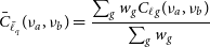 \begin{equation}\bar{C}_{\bar{\ell}_q}(\nu_a,\nu_b) = \frac{ \sum_g w_g C_{\ell}{_g}(\nu_a,\nu_b)}{ \sum_g w_g}\end{equation}
where $ \bar{C}_{\bar{\ell}_q}(\nu_a,\nu_b)$
is the bin averaged MAPS at
$ \bar{C}_{\bar{\ell}_q}(\nu_a,\nu_b)$
is the bin averaged MAPS at
 \begin{equation}\bar{\ell}_q =\frac{ \sum_g w_g \ell_g}{ \sum_g w_g}\end{equation}
which is the effective angular multipole for bin $q$
. For brevity of notation, we use
$q$
. For brevity of notation, we use $C_{\ell}(\nu_a,\nu_b)$
instead of
$C_{\ell}(\nu_a,\nu_b)$
instead of $\bar{C}_{\bar{\ell}_q}(\nu_a,\nu_b)$
in the subsequent discussion.
$\bar{C}_{\bar{\ell}_q}(\nu_a,\nu_b)$
in the subsequent discussion.
For the subsequent analysis, we assume that the 21-cm signal is statistically homogeneous (ergodic) along the line of sight whereby $C_{\ell}(\nu_a, \nu_b) = C_{\ell}(\Delta\nu)$
(equation (4)). Such an assumption is valid for the redshifted 21-cm signal if the observing bandwidth
$C_{\ell}(\nu_a, \nu_b) = C_{\ell}(\Delta\nu)$
(equation (4)). Such an assumption is valid for the redshifted 21-cm signal if the observing bandwidth $B_w$
is sufficiently small (
$B_w$
is sufficiently small ( $\approx$ $8 \, \mathrm{MHz}$
; Mondal et al. Reference Mondal, Bharadwaj and Datta2018) such that the mean neutral hydrogen fraction does not evolve significantly across the corresponding redshift interval. Although
$8 \, \mathrm{MHz}$
; Mondal et al. Reference Mondal, Bharadwaj and Datta2018) such that the mean neutral hydrogen fraction does not evolve significantly across the corresponding redshift interval. Although $B_w = 30.72 \, \mathrm{MHz}$
used here is quite a bit larger and we may expect some signal loss at the small
$B_w = 30.72 \, \mathrm{MHz}$
used here is quite a bit larger and we may expect some signal loss at the small $k$
, we still adopt this assumption as it significantly simplifies the analysis as we can quantify the signal using
$k$
, we still adopt this assumption as it significantly simplifies the analysis as we can quantify the signal using $P(k_{\perp},\,k_{\parallel})$
the cylindrical PS of the 21-cm brightness temperature fluctuations which is related to a
$P(k_{\perp},\,k_{\parallel})$
the cylindrical PS of the 21-cm brightness temperature fluctuations which is related to a $C_{\ell}(\Delta \nu)$
through a Fourier transform. We have (Datta et al. Reference Datta, Choudhury and Bharadwaj2007)
$C_{\ell}(\Delta \nu)$
through a Fourier transform. We have (Datta et al. Reference Datta, Choudhury and Bharadwaj2007)
 \begin{equation} P(k_{\perp},\,k_{\parallel})= r^2\,r^{\prime} \int_{-\infty}^{\infty} d (\Delta \nu) \, e^{-i k_{\parallel} r^{\prime} \Delta \nu}\, C_{\ell}(\Delta \nu) \end{equation}
where $k_{\parallel}$
(the Fourier conjugate of
$k_{\parallel}$
(the Fourier conjugate of $\Delta \nu$
) and and
$\Delta \nu$
) and and $k_{\perp}=\ell/r$
are component of
$k_{\perp}=\ell/r$
are component of $\textbf{k}$
, respectively, parallel and perpendicular to the line of sight. Here,
$\textbf{k}$
, respectively, parallel and perpendicular to the line of sight. Here, $r = 9\,210 \,\mathrm{Mpc}$
is the comoving distance corresponding to
$r = 9\,210 \,\mathrm{Mpc}$
is the comoving distance corresponding to $\nu_c$
and
$\nu_c$
and $r^{\prime}=d r/d \nu = 16.99 \,\mathrm{Mpc\, MHz}^{-1}$
evaluated at
$r^{\prime}=d r/d \nu = 16.99 \,\mathrm{Mpc\, MHz}^{-1}$
evaluated at $\nu_c$
. The reader is referred to Bharadwaj et al. (Reference Bharadwaj, Pal, Choudhuri and Dutta2018) for further details.
$\nu_c$
. The reader is referred to Bharadwaj et al. (Reference Bharadwaj, Pal, Choudhuri and Dutta2018) for further details.
To proceed further with the TTGE, we have collapsed the measured $C_{\ell}(\nu_a, \nu_b)$
to obtain
$C_{\ell}(\nu_a, \nu_b)$
to obtain $C(\Delta \nu_n)$
where
$C(\Delta \nu_n)$
where $\Delta \nu_n =n \, \Delta \nu_c$
with
$\Delta \nu_n =n \, \Delta \nu_c$
with $n=0,1,2,\ldots,N_c-1$
. We then use a maximum likelihood estimator (MLE; Pal et al. Reference Pal2022) to obtain the cylindrical PS
$n=0,1,2,\ldots,N_c-1$
. We then use a maximum likelihood estimator (MLE; Pal et al. Reference Pal2022) to obtain the cylindrical PS
 \begin{equation} P(k_{\perp}, k_{\parallel q}) = \sum_n \left[ \left(\textbf{A} ^{\dagger} \textbf{N}^{-1} \textbf{A}\right)^{-1} \textbf{A}^{\dagger} \textbf{N}^{-1} \right]_{qn} \mathcal{W}(\Delta\nu_n) \, C_{\ell}(\Delta\nu_n) \end{equation}
where the Hermitian matrix $\textbf{A}$
contains the Fourier coefficients and
$\textbf{A}$
contains the Fourier coefficients and $\textbf{N}$
is the noise covariance matrix. We have assumed
$\textbf{N}$
is the noise covariance matrix. We have assumed $\textbf{N}$
to be diagonal and estimated it using noise only simulations. In these simulations the real and imaginary parts of the measured visibilites were both replaced with Gaussian random noise of variance
$\textbf{N}$
to be diagonal and estimated it using noise only simulations. In these simulations the real and imaginary parts of the measured visibilites were both replaced with Gaussian random noise of variance $\unicode{x03C3}_\mathrm{N}^2$
. These simulated data were run through the TTGE pipeline to estimate
$\unicode{x03C3}_\mathrm{N}^2$
. These simulated data were run through the TTGE pipeline to estimate $C_{\ell}(\Delta\nu_n)$
, and we have used 20 realisations of the simulated visibilities to estimate
$C_{\ell}(\Delta\nu_n)$
, and we have used 20 realisations of the simulated visibilities to estimate $[\unicode{x03B4} C_{\ell}(\Delta\nu_n)]^2$
the variance of
$[\unicode{x03B4} C_{\ell}(\Delta\nu_n)]^2$
the variance of $C_{\ell}(\Delta\nu_n)$
which are the diagonal elements of
$C_{\ell}(\Delta\nu_n)$
which are the diagonal elements of $\textbf{N}$
. Note that TTGE avoids the noise bias, and the mean
$\textbf{N}$
. Note that TTGE avoids the noise bias, and the mean $C_{\ell}(\Delta\nu_n)$
is expected to be zero for noise only simulations.
$C_{\ell}(\Delta\nu_n)$
is expected to be zero for noise only simulations.
The window function $\mathcal{W}(\Delta\nu_n)$
, which is normalised to unity at
$\mathcal{W}(\Delta\nu_n)$
, which is normalised to unity at $\Delta\nu = 0$
, is used to avoid a discontinuity in the measured
$\Delta\nu = 0$
, is used to avoid a discontinuity in the measured $C_{\ell}(\Delta\nu_n)$
at the band edges. For the present work we have used a Blackman–Nuttall (BN; Nuttall Reference Nuttall1981) window function.
$C_{\ell}(\Delta\nu_n)$
at the band edges. For the present work we have used a Blackman–Nuttall (BN; Nuttall Reference Nuttall1981) window function.
4. Validating the TTGE
4.1 All-sky simulation
The aim here is to simulate the visibilities that would be measured in MWA drift scan observations of $T(\hat{\textbf{n}},\nu)$
the redshifted 21-cm brightness temperature distribution on the sky. We simulate
$T(\hat{\textbf{n}},\nu)$
the redshifted 21-cm brightness temperature distribution on the sky. We simulate $T(\hat{\textbf{n}},\nu)$
using the package HEALPix (Hierarchical Equal Area isoLatitude Pixelization of a sphere; Gorski et al. Reference Gorski2005). For the simulations presented here, we have set
$T(\hat{\textbf{n}},\nu)$
using the package HEALPix (Hierarchical Equal Area isoLatitude Pixelization of a sphere; Gorski et al. Reference Gorski2005). For the simulations presented here, we have set $N_\mathrm{side}=512$
in HEALPix, which results in
$N_\mathrm{side}=512$
in HEALPix, which results in $\ell_{max}= 1\,535$
and a pixel size of
$\ell_{max}= 1\,535$
and a pixel size of $6.87^{'}$
.
$6.87^{'}$
.
We assume $T(\hat{\textbf{n}},\nu)$
to be a GRF with a given input model PS
$T(\hat{\textbf{n}},\nu)$
to be a GRF with a given input model PS $P^m (k_{\perp}, k_{\parallel})$
. To simulate the signal, we consider
$P^m (k_{\perp}, k_{\parallel})$
. To simulate the signal, we consider
 \begin{equation} C_{\ell}(\Delta\nu_n) = \frac{1}{N_c \Delta\nu_c \, r^2\,r^{\prime}} \sum_{q=0}^{N_c-1} P(k_{\perp}, k_{\parallel q}) \, e^{2 \pi i n q /N_c} \, \end{equation}
which is the discrete representation of the inverse of equation (16). We generate the expansion coefficients $a_{\ell}^{m}(\nu_n)$
at the
$a_{\ell}^{m}(\nu_n)$
at the $n$
-th frequency channel (equation (3)) using
$n$
-th frequency channel (equation (3)) using
 \begin{equation} a_{\ell}^{m}(\nu_n) = \sum_{q=0}^{N_c-1} \left[ \sqrt{\frac{P^m(k_{\perp}, k_{\parallel q})}{N_c \Delta\nu_c \, r^2 \, r^{\prime} }} \left( \frac{\hat{\textbf{x}}_q + i \hat{\textbf{y}}_q}{\sqrt{2}} \right)\right]\, e^{\frac{2 \pi i n q}{N_c}} \, \end{equation}
where $\hat{\textbf{x}}_q,\hat{\textbf{y}}_q$
are independent Gaussian random variables of unit variance and use equation (2) to calculate
$\hat{\textbf{x}}_q,\hat{\textbf{y}}_q$
are independent Gaussian random variables of unit variance and use equation (2) to calculate $T(\hat{\textbf{n}},\nu_n)$
. We now use equation (4) of Reference Chatterjee, Bharadwaj, Choudhuri, Sethi and PatwaPaper I to calculate the simulated visibilities
$T(\hat{\textbf{n}},\nu_n)$
. We now use equation (4) of Reference Chatterjee, Bharadwaj, Choudhuri, Sethi and PatwaPaper I to calculate the simulated visibilities $\mathcal{V}(\alpha_p,\textbf{U}_i,\nu_a)$
for all the PCs covered in the actual data. Note that we have simulated the visibilities for the same baseline distribution, frequency channels, and flagging of the actual data. For the present work, we have assumed the model PS to be
$\mathcal{V}(\alpha_p,\textbf{U}_i,\nu_a)$
for all the PCs covered in the actual data. Note that we have simulated the visibilities for the same baseline distribution, frequency channels, and flagging of the actual data. For the present work, we have assumed the model PS to be
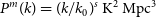 \begin{equation} P^m (k) = (k/k_0 )^s \, \mathrm{K}^2 \, \mathrm{Mpc}^3 \,\end{equation}
with $k_0 =1 \, \mathrm{Mpc}^{-1}$
and
$k_0 =1 \, \mathrm{Mpc}^{-1}$
and $s = -1$
. We have used 20 independent relaisations of the simulated signal to estimate the mean and
$s = -1$
. We have used 20 independent relaisations of the simulated signal to estimate the mean and $1 \unicode{x03C3}$
errors for all the results presented below.
$1 \unicode{x03C3}$
errors for all the results presented below.
In order to simulate the sky signal corresponding to UMAPS, we first consider a fixed frequency channel (say $n=0$
) and generate a GRF
$n=0$
) and generate a GRF $T(\hat{\textbf{n}},\nu_0)$
corresponding to a unit angular PS
$T(\hat{\textbf{n}},\nu_0)$
corresponding to a unit angular PS $C_{\ell}=1$
. We then assign the same brightness temperature map to all the other frequency channels within our observing bandwidth, that is,
$C_{\ell}=1$
. We then assign the same brightness temperature map to all the other frequency channels within our observing bandwidth, that is, $T(\hat{\textbf{n}},\nu_n)=T(\hat{\textbf{n}},\nu_0)$
for
$T(\hat{\textbf{n}},\nu_n)=T(\hat{\textbf{n}},\nu_0)$
for $n = 1,2,3,\ldots,N_c-1$
. This ensures that the simulated sky signal
$n = 1,2,3,\ldots,N_c-1$
. This ensures that the simulated sky signal $T(\hat{\textbf{n}},\nu_n)$
corresponds to
$T(\hat{\textbf{n}},\nu_n)$
corresponds to $C_{\ell}(\nu_a,\nu_b)=1$
(UMAPS). The UMAPS visibilities
$C_{\ell}(\nu_a,\nu_b)=1$
(UMAPS). The UMAPS visibilities $ [\mathcal{V}(\alpha_p,\textbf{U}_i,\nu_a)]_\mathrm{UMAPS}$
were simulated using HEALPix exactly the same way as for the model PS, with the exception that the sky signal is different. As mentioned earlier, we have used 100 realisations of UMAPS to estimate
$ [\mathcal{V}(\alpha_p,\textbf{U}_i,\nu_a)]_\mathrm{UMAPS}$
were simulated using HEALPix exactly the same way as for the model PS, with the exception that the sky signal is different. As mentioned earlier, we have used 100 realisations of UMAPS to estimate $M_g(\nu_a,\nu_b)$
.
$M_g(\nu_a,\nu_b)$
.
We have introduced noise in the simulations as a GRF with zero mean and standard deviation $\unicode{x03C3}_\mathrm{N} = 10 \, \mathrm{Jy}$
. This is equivalent to an observation where
$\unicode{x03C3}_\mathrm{N} = 10 \, \mathrm{Jy}$
. This is equivalent to an observation where $N_\mathrm{nights} = 36$
(equation (1)) and sets the
$N_\mathrm{nights} = 36$
(equation (1)) and sets the $\mathrm{SNR}\,{=}\,3$
at the smallest
$\mathrm{SNR}\,{=}\,3$
at the smallest $k$
-bin for the input model considered here. The actual EoR signal is significantly fainter and requires much longer observations for a detection.
$k$
-bin for the input model considered here. The actual EoR signal is significantly fainter and requires much longer observations for a detection.
4.2 Single pointing
In this subsection, and also the subsequent subsection, we use the simulated visibilities to validate the TTGE considering a single TC at $(\mathrm{RA,DEC)} = (6.1^{\circ},-26.7^{\circ})$
. We have used a window function (equation (7))
$(\mathrm{RA,DEC)} = (6.1^{\circ},-26.7^{\circ})$
. We have used a window function (equation (7)) $ W\left(\unicode{x1D6C9} \right)=e^{-\unicode{x03B8}^2/\unicode{x03B8}_w^2}$
where
$ W\left(\unicode{x1D6C9} \right)=e^{-\unicode{x03B8}^2/\unicode{x03B8}_w^2}$
where $\unicode{x03B8}_w =0.6 \, \unicode{x03B8}_\mathrm{FWHM}$
with
$\unicode{x03B8}_w =0.6 \, \unicode{x03B8}_\mathrm{FWHM}$
with $\unicode{x03B8}_\mathrm{FWHM} = 15^{\circ}$
. This effectively restricts the sky signal to an angular region of extent
$\unicode{x03B8}_\mathrm{FWHM} = 15^{\circ}$
. This effectively restricts the sky signal to an angular region of extent $\sim 15^{\circ}$
centred around the TC, and this remains fixed even as the pointing centre PC drifts across the sky. In this section, we have considered a single PC (=34) which exactly coincides with the TC. Note that the simulations used here do not contain any system noise.
$\sim 15^{\circ}$
centred around the TC, and this remains fixed even as the pointing centre PC drifts across the sky. In this section, we have considered a single PC (=34) which exactly coincides with the TC. Note that the simulations used here do not contain any system noise.
Fig. 3 shows the estimated MAPS $C_{\ell}(\Delta\nu)$
along with the model predictions
$C_{\ell}(\Delta\nu)$
along with the model predictions $C_{\ell}^\mathrm{M}(\Delta\nu)$
. Note that the range
$C_{\ell}^\mathrm{M}(\Delta\nu)$
. Note that the range $ 50 \lt \ell \lt 1\,493 $
has been divided into 20
$ 50 \lt \ell \lt 1\,493 $
has been divided into 20 $\ell$
bins, and the results are shown for four representative bins. We see that model predictions are within the
$\ell$
bins, and the results are shown for four representative bins. We see that model predictions are within the $1 \unicode{x03C3}$
error bars of the estimated
$1 \unicode{x03C3}$
error bars of the estimated $C_{\ell}(\Delta\nu)$
, indicating that the two are in good agreement. It is important to note that the estimated
$C_{\ell}(\Delta\nu)$
, indicating that the two are in good agreement. It is important to note that the estimated $C_{\ell}(\Delta\nu)$
shows a smooth
$C_{\ell}(\Delta\nu)$
shows a smooth $\Delta \nu$
dependence with no missing frequency separations
$\Delta \nu$
dependence with no missing frequency separations $\Delta \nu$
. In particular, we do not see any artefacts in the estimated
$\Delta \nu$
. In particular, we do not see any artefacts in the estimated $C_{\ell}(\Delta\nu)$
due to the periodic pattern of flagged channels present in the simulations (Fig. 2).
$C_{\ell}(\Delta\nu)$
due to the periodic pattern of flagged channels present in the simulations (Fig. 2).
This shows $C_{\ell}(\Delta\nu)$
as a function of
$C_{\ell}(\Delta\nu)$
as a function of $\Delta\nu$
for four values of
$\Delta\nu$
for four values of $\ell$
. The data points with
$\ell$
. The data points with $1\unicode{x03C3}$
error bars are estimated from 20 realisations of the all-sky simulations. The lines show the theoretical predictions calculated using the input model power spectrum
$1\unicode{x03C3}$
error bars are estimated from 20 realisations of the all-sky simulations. The lines show the theoretical predictions calculated using the input model power spectrum $P^m(k)=(1 \mathrm{Mpc}^{-1}/k) \, \mathrm{K^2}\, \mathrm{Mpc^3}$
in equation (16). The
$P^m(k)=(1 \mathrm{Mpc}^{-1}/k) \, \mathrm{K^2}\, \mathrm{Mpc^3}$
in equation (16). The $\Delta\nu = 0$
points have been slightly shifted for the convenience of plotting on a logarithmic scale.
$\Delta\nu = 0$
points have been slightly shifted for the convenience of plotting on a logarithmic scale.

The left panel of Fig. 4 shows the cylindrical PS $P(k_{\perp}, k_{\parallel})$
estimated from the
$P(k_{\perp}, k_{\parallel})$
estimated from the $C_{\ell}(\Delta\nu)$
shown in Fig. 3 using equation (17). For comparison, the right panel shows
$C_{\ell}(\Delta\nu)$
shown in Fig. 3 using equation (17). For comparison, the right panel shows $P(k_{\perp}, k_{\parallel})$
estimated using identical simulations which do not incorporate the channel flagging. We note that the
$P(k_{\perp}, k_{\parallel})$
estimated using identical simulations which do not incorporate the channel flagging. We note that the $P(k_{\perp}, k_{\parallel})$
shown in the two panels are visually indistinguishable. Several earlier works which have first transformed from frequency to delay space and then estimated the PS (e.g. Paul et al. Reference Paul2016; Li et al. Reference Li2019; Trott et al. Reference Trott2020; Patwa et al. Reference Patwa, Sethi and Dwarakanath2021) have reported horizontal streaks in the estimated
$P(k_{\perp}, k_{\parallel})$
shown in the two panels are visually indistinguishable. Several earlier works which have first transformed from frequency to delay space and then estimated the PS (e.g. Paul et al. Reference Paul2016; Li et al. Reference Li2019; Trott et al. Reference Trott2020; Patwa et al. Reference Patwa, Sethi and Dwarakanath2021) have reported horizontal streaks in the estimated $P(k_{\perp}, k_{\parallel})$
due to the periodic pattern of flagged channels present in the MWA data. In our approach (Bharadwaj et al. Reference Bharadwaj, Pal, Choudhuri and Dutta2018), we first estimate
$P(k_{\perp}, k_{\parallel})$
due to the periodic pattern of flagged channels present in the MWA data. In our approach (Bharadwaj et al. Reference Bharadwaj, Pal, Choudhuri and Dutta2018), we first estimate $C_{\ell}(\Delta\nu)$
, which does not have any missing
$C_{\ell}(\Delta\nu)$
, which does not have any missing $\Delta\nu$
even when the visibility data contains flagged channels. We then Fourier transform
$\Delta\nu$
even when the visibility data contains flagged channels. We then Fourier transform $C_{\ell}(\Delta\nu)$
to obtain a clean estimate of
$C_{\ell}(\Delta\nu)$
to obtain a clean estimate of $P(k_{\perp}, k_{\parallel})$
. We see that the missing frequency channels do not introduce any artefacts in the estimated
$P(k_{\perp}, k_{\parallel})$
. We see that the missing frequency channels do not introduce any artefacts in the estimated $P(k_{\perp}, k_{\parallel})$
.
$P(k_{\perp}, k_{\parallel})$
.
Left panel shows the cylindrical power spectrum $P(k_{\perp}, k_{\parallel})$
estimated from simulations with MWA coarse channel flagging. For comparison, the right panel shows the
$P(k_{\perp}, k_{\parallel})$
estimated from simulations with MWA coarse channel flagging. For comparison, the right panel shows the $P(k_{\perp}, k_{\parallel})$
estimated from simulations without coarse channel flagging. We do not notice any significant difference.
$P(k_{\perp}, k_{\parallel})$
estimated from simulations without coarse channel flagging. We do not notice any significant difference.

The top panel of Fig. 5 shows $P(k)$
the spherical PS estimated directly from the
$P(k)$
the spherical PS estimated directly from the $C_{\ell}(\Delta\nu)$
shown in Fig. 3 using an MLE (Elahi et al. Reference Elahi2023a), for comparison we also show
$C_{\ell}(\Delta\nu)$
shown in Fig. 3 using an MLE (Elahi et al. Reference Elahi2023a), for comparison we also show $P^m(k)$
the input model PS. We see that the model predictions
$P^m(k)$
the input model PS. We see that the model predictions $P^m(k)$
are within the
$P^m(k)$
are within the $1 \unicode{x03C3}$
error bars of the estimated
$1 \unicode{x03C3}$
error bars of the estimated $P(k)$
, indicating that the two are in good agreement through the entire
$P(k)$
, indicating that the two are in good agreement through the entire $k$
range 0.01–4
$k$
range 0.01–4 $\mathrm{Mpc}^{-1}$
probed here. We have quantified the percentage deviation between
$\mathrm{Mpc}^{-1}$
probed here. We have quantified the percentage deviation between $P(k)$
and
$P(k)$
and $P^m(k)$
using
$P^m(k)$
using $\Delta = [P(k) - P^m(k)]/P^m(k) \times 100$
shown in the second panel (from top) of Fig. 5. We see that for nearly all
$\Delta = [P(k) - P^m(k)]/P^m(k) \times 100$
shown in the second panel (from top) of Fig. 5. We see that for nearly all $k$
the values of
$k$
the values of $\Delta$
are within the predicted
$\Delta$
are within the predicted $1 \unicode{x03C3}$
error bars. The values of
$1 \unicode{x03C3}$
error bars. The values of $\mid \Delta \mid$
are within
$\mid \Delta \mid$
are within $1 \%$
for
$1 \%$
for $k \ge 0.13 \, \mathrm{ Mpc^{-1}}$
and within
$k \ge 0.13 \, \mathrm{ Mpc^{-1}}$
and within $2 \%$
for
$2 \%$
for $k \ge 0.035 \, \mathrm{ Mpc^{-1}}$
. We see that
$k \ge 0.035 \, \mathrm{ Mpc^{-1}}$
. We see that $\mid \Delta \mid$
increases at smaller
$\mid \Delta \mid$
increases at smaller $k$
due to the convolution with the window function and the PB pattern. We have the largest deviation
$k$
due to the convolution with the window function and the PB pattern. We have the largest deviation $|\Delta| = 6.9 \%$
at
$|\Delta| = 6.9 \%$
at $ k = 0.013 \, \mathrm{Mpc^{-1}} $
. Overall, we find very good agreement between
$ k = 0.013 \, \mathrm{Mpc^{-1}} $
. Overall, we find very good agreement between $P(k)$
and
$P(k)$
and $P^m(k)$
. Further, we do not find any artefacts due to the periodic pattern of flagged channels present in the MWA data.
$P^m(k)$
. Further, we do not find any artefacts due to the periodic pattern of flagged channels present in the MWA data.
The upper panel shows the estimated spherically binned power spectrum $P(k)$
and
$P(k)$
and $1-\unicode{x03C3}$
error bars for simulations for PC=34 with no noise and coarse channel flagging. For comparison, the input model
$1-\unicode{x03C3}$
error bars for simulations for PC=34 with no noise and coarse channel flagging. For comparison, the input model $P^m(k)=(1 \mathrm{Mpc}^{-1}/k) \, \mathrm{K^2}\, \mathrm{Mpc^3}$
is also shown by the solid line. The lower panels show the percentage error
$P^m(k)=(1 \mathrm{Mpc}^{-1}/k) \, \mathrm{K^2}\, \mathrm{Mpc^3}$
is also shown by the solid line. The lower panels show the percentage error $\Delta= [P(k) - P^m (k)]/P^m (k)$
(data points) and the relative statistical fluctuation
$\Delta= [P(k) - P^m (k)]/P^m (k)$
(data points) and the relative statistical fluctuation $\unicode{x03C3} /P^m (k) \times 100 \%$
(between the solid lines). The four lower panels consider situations for combining different PCs mentioned in the figure legends.
$\unicode{x03C3} /P^m (k) \times 100 \%$
(between the solid lines). The four lower panels consider situations for combining different PCs mentioned in the figure legends.

The flagged channels present in the MWA data cause $\sim 28 \%$
data loss, and we expect this to degrade the SNR of the 21-cm PS relative to the situation when there are no flagged channels. The upper panel of Fig. 6 shows a comparison of the SNR for the 21-cm PS estimated from the simulations with (squares) and without (circles) the periodic pattern of flagged channels. In the absence of flagging, the SNR has value
$\sim 28 \%$
data loss, and we expect this to degrade the SNR of the 21-cm PS relative to the situation when there are no flagged channels. The upper panel of Fig. 6 shows a comparison of the SNR for the 21-cm PS estimated from the simulations with (squares) and without (circles) the periodic pattern of flagged channels. In the absence of flagging, the SNR has value $\sim$
4 at the smallest
$\sim$
4 at the smallest $k$
bin and rises monotonically to
$k$
bin and rises monotonically to $\sim$
300 at the largest
$\sim$
300 at the largest $k$
bin. The results with flagging are similar, but the SNR values are somewhat smaller. The lower panel shows the ratio of the SNR without flagging to with flagging. We find that the ratio is very close to unity at
$k$
bin. The results with flagging are similar, but the SNR values are somewhat smaller. The lower panel shows the ratio of the SNR without flagging to with flagging. We find that the ratio is very close to unity at $k \lt 0.09 \, \mathrm{Mpc}^{-1}$
, and the ratio increases only at large
$k \lt 0.09 \, \mathrm{Mpc}^{-1}$
, and the ratio increases only at large $k$
where it varies in the range 1–2. We find that The ratio has a maximum value
$k$
where it varies in the range 1–2. We find that The ratio has a maximum value $(\sim$
2) at
$(\sim$
2) at $k\sim 0.5 \, \mathrm{Mpc}^{-1}$
. Note that the discussion, till now, has not considered the system noise. The upper panel of Fig. 6 also shows the SNR for the simulations which include the system noise. We see that the SNR at the two smallest
$k\sim 0.5 \, \mathrm{Mpc}^{-1}$
. Note that the discussion, till now, has not considered the system noise. The upper panel of Fig. 6 also shows the SNR for the simulations which include the system noise. We see that the SNR at the two smallest $k$
bins are not much affected even if we introduce the system noise. The total noise budget in these two bins is dominated by the cosmic variance (CV), and the system noise make only a small contribution. We find that there is a very substantial drop in the SNR at the larger
$k$
bins are not much affected even if we introduce the system noise. The total noise budget in these two bins is dominated by the cosmic variance (CV), and the system noise make only a small contribution. We find that there is a very substantial drop in the SNR at the larger $k$
bins when we introduce the system noise. There is very little difference in the SNR between with and without flagging once we introduce the system noise contribution.
$k$
bins when we introduce the system noise. There is very little difference in the SNR between with and without flagging once we introduce the system noise contribution.
The upper panel shows a comparison of SNR achievable for a single pointing with (circles) and without (squares) the periodic pattern of flagged channels. The triangles show the expected SNR values in the presence of system noise with $\unicode{x03C3}_\mathrm{N} = 10 \, \mathrm{Jy}$
(equation (1)). The lower panel shows the ratio of the SNR values without and with flagging. The shaded region indicates the
$\unicode{x03C3}_\mathrm{N} = 10 \, \mathrm{Jy}$
(equation (1)). The lower panel shows the ratio of the SNR values without and with flagging. The shaded region indicates the $k$
-range where the SNR values remain mostly unaffected due to flagging.
$k$
-range where the SNR values remain mostly unaffected due to flagging.

4.3 Multiple pointings
In this subsection we coherently combine the visibilities measured at multiple PCs to estimate the signal in a small angular region centred at the fixed TC $\hat{\textbf{c}}$
whose sky coordinates we have mentioned in the previous subsection. As mentioned earlier, the contribution from a PC declines as
$\hat{\textbf{c}}$
whose sky coordinates we have mentioned in the previous subsection. As mentioned earlier, the contribution from a PC declines as $\sim A\left(-\unicode{x1D6D8}_p,\nu\right)$
(equation (7)) as the separation
$\sim A\left(-\unicode{x1D6D8}_p,\nu\right)$
(equation (7)) as the separation $\unicode{x1D6D8}_p=\hat{\textbf{p}}-\hat{\textbf{c}}$
increases. The PC which are close to the TC contribute to
$\unicode{x1D6D8}_p=\hat{\textbf{p}}-\hat{\textbf{c}}$
increases. The PC which are close to the TC contribute to $\mathcal{V}_{cg}(\nu_a)$
with the higher SNR as compared to the PC which are at a large angular separation, and we account for this by suitably choosing the factor
$\mathcal{V}_{cg}(\nu_a)$
with the higher SNR as compared to the PC which are at a large angular separation, and we account for this by suitably choosing the factor $s_p$
(equation (9)).
$s_p$
(equation (9)).
In the previous subsection, we have considered a single pointing centre PC=34 which exactly coincides with the TC, that is, $\hat{\textbf{p}}=\hat{\textbf{c}}$
and
$\hat{\textbf{p}}=\hat{\textbf{c}}$
and $\unicode{x1D6D8}_p=0$
. In this subsection we consider other pointing directions PC=34 +
$\unicode{x1D6D8}_p=0$
. In this subsection we consider other pointing directions PC=34 + $\Delta$
PC. Before combining the signal from multiple pointing directions, we analyse how the correlation between the signal from two different pointing directions PC=34 and PC=34 +
$\Delta$
PC. Before combining the signal from multiple pointing directions, we analyse how the correlation between the signal from two different pointing directions PC=34 and PC=34 + $\Delta$
PC changes as
$\Delta$
PC changes as $\Delta \, \mathrm{PC} $
is varied. To evaluate this we consider the dimensionless correlation coefficient
$\Delta \, \mathrm{PC} $
is varied. To evaluate this we consider the dimensionless correlation coefficient
 \begin{equation} c_{\ell}(\Delta \, \mathrm{PC}) = [C_{\ell}(0)]_{\Delta \, \mathrm{PC}} /C_{\ell}(0) \end{equation}
where we have evaluated $[C_{\ell}(0)]_{\Delta \, \mathrm{PC}}$
using eqution (10) with the difference that
$[C_{\ell}(0)]_{\Delta \, \mathrm{PC}}$
using eqution (10) with the difference that $\mathcal{V}_{cg}(\nu_a) $
and
$\mathcal{V}_{cg}(\nu_a) $
and $ \mathcal{V}^*_{cg}(\nu_b)$
refer to PC=34 and PC=34 +
$ \mathcal{V}^*_{cg}(\nu_b)$
refer to PC=34 and PC=34 + $\Delta$
PC, respectively. Note that these simulations do not contain system noise, and it is not necessary to subtract out the self-correlation in equation (10).
$\Delta$
PC, respectively. Note that these simulations do not contain system noise, and it is not necessary to subtract out the self-correlation in equation (10).
Fig. 7 shows $c_{\ell}(\Delta \, \mathrm{PC}) $
as a function of
$c_{\ell}(\Delta \, \mathrm{PC}) $
as a function of $\ell$
for different values of
$\ell$
for different values of $\Delta \, \mathrm{PC}$
in the range 1–5. We see that in all cases, the correlation drops as
$\Delta \, \mathrm{PC}$
in the range 1–5. We see that in all cases, the correlation drops as $\Delta \, \mathrm{PC} $
, the offset between TC and PC, is increased. This is roughly consistent with the expected
$\Delta \, \mathrm{PC} $
, the offset between TC and PC, is increased. This is roughly consistent with the expected $\sim A\left(-\unicode{x1D6D8}_p,\nu\right)$
(equation (7)) decline, and also the finding of Patwa & Sethi (Reference Patwa and Sethi2019). This analysis sets the choice for combining different PC later in the analysis.
$\sim A\left(-\unicode{x1D6D8}_p,\nu\right)$
(equation (7)) decline, and also the finding of Patwa & Sethi (Reference Patwa and Sethi2019). This analysis sets the choice for combining different PC later in the analysis.
This shows a measure of visibility correlation between two different PCs for a fixed TC. The correlation = $C_{\ell}(\Delta\nu=0, \Delta \mathrm{PC})/C_{\ell}(\Delta\nu=0, \Delta \mathrm{PC}=0)$
. Here, we have fixed the TC at PC=34 and estimated the MAPS
$C_{\ell}(\Delta\nu=0, \Delta \mathrm{PC})/C_{\ell}(\Delta\nu=0, \Delta \mathrm{PC}=0)$
. Here, we have fixed the TC at PC=34 and estimated the MAPS $C_{\ell}(\Delta\nu)$
by correlating visibilities separated by
$C_{\ell}(\Delta\nu)$
by correlating visibilities separated by $\Delta \mathrm{PC}$
pointing centres. Here, we only show the results for
$\Delta \mathrm{PC}$
pointing centres. Here, we only show the results for $\Delta\nu = 0$
, however,
$\Delta\nu = 0$
, however, $\Delta\nu > 0$
results are quite similar.
$\Delta\nu > 0$
results are quite similar.

Considering $\Delta \, \mathrm{PC}=1$
, we see that
$\Delta \, \mathrm{PC}=1$
, we see that $c_{\ell}(\Delta \, \mathrm{PC}) \approx 1$
for
$c_{\ell}(\Delta \, \mathrm{PC}) \approx 1$
for $\ell \le 300$
, it is
$\ell \le 300$
, it is $>0.9$
for
$>0.9$
for $\ell \le 800$
and it drops at larger
$\ell \le 800$
and it drops at larger $\ell$
to
$\ell$
to $\sim 0.8$
at
$\sim 0.8$
at $\ell = 2\,000$
. We find a similar behaviour for larger
$\ell = 2\,000$
. We find a similar behaviour for larger $ \Delta \, \mathrm{PC}$
, but the values of
$ \Delta \, \mathrm{PC}$
, but the values of $c_{\ell}(\Delta \, \mathrm{PC}) $
are smaller. Overall, the signal at small
$c_{\ell}(\Delta \, \mathrm{PC}) $
are smaller. Overall, the signal at small $\ell \, (\le 300)$
remains correlated for large
$\ell \, (\le 300)$
remains correlated for large $\Delta \, \mathrm{PC}$
, even beyond 5. However, at larger
$\Delta \, \mathrm{PC}$
, even beyond 5. However, at larger $\ell$ $(> 800)$
the correlation falls below
$(> 800)$
the correlation falls below $\sim 0.7$
for
$\sim 0.7$
for $ \Delta \, \mathrm{PC} \ge 3$
. We have also investigated
$ \Delta \, \mathrm{PC} \ge 3$
. We have also investigated $c_{\ell}(\Delta \, \mathrm{PC}) $
for other values of
$c_{\ell}(\Delta \, \mathrm{PC}) $
for other values of $\Delta \nu$
(equation (21)), and we find that the behaviour is very similar to that for
$\Delta \nu$
(equation (21)), and we find that the behaviour is very similar to that for $\Delta \nu=0$
shown here. We note that the variation of
$\Delta \nu=0$
shown here. We note that the variation of $c_{\ell}(\Delta \, \mathrm{PC}) $
with
$c_{\ell}(\Delta \, \mathrm{PC}) $
with $\Delta \, \mathrm{PC}$
depends on the width of the window function where we have used
$\Delta \, \mathrm{PC}$
depends on the width of the window function where we have used $\unicode{x03B8}_\mathrm{FWHM} = 15^{\circ}$
, and we expect the correlation to decrease faster with
$\unicode{x03B8}_\mathrm{FWHM} = 15^{\circ}$
, and we expect the correlation to decrease faster with $ \Delta \, \mathrm{PC}$
if
$ \Delta \, \mathrm{PC}$
if $\unicode{x03B8}_\mathrm{FWHM}$
is reduced.
$\unicode{x03B8}_\mathrm{FWHM}$
is reduced.
The results shown in Fig. 7 indicate that it is most optimal to consider the weights $s_p$
in equation (9) as functions of
$s_p$
in equation (9) as functions of $\ell$
. However, we have not considered this here. We have considered three simple schemes where we use uniform weights
$\ell$
. However, we have not considered this here. We have considered three simple schemes where we use uniform weights $s_p=1$
to combine multiple pointings. In the first scheme we combine PC=33, 34, and 35 (33-35) for which the maximum
$s_p=1$
to combine multiple pointings. In the first scheme we combine PC=33, 34, and 35 (33-35) for which the maximum $ \mid \Delta \, \mathrm{PC} \mid $
has value 1. We similarly also consider PC= 32-36 and 31-37 for which the maximum
$ \mid \Delta \, \mathrm{PC} \mid $
has value 1. We similarly also consider PC= 32-36 and 31-37 for which the maximum $ \mid \Delta \, \mathrm{PC} \mid$
has values 2 and 3, respectively. The correlation at large
$ \mid \Delta \, \mathrm{PC} \mid$
has values 2 and 3, respectively. The correlation at large $\ell$
falls considerably for
$\ell$
falls considerably for $ \mid \Delta \, \mathrm{PC} \mid \ge 4$
, and we have not considered combining such pointings. Considering PC=31-37, the RA difference between PC=31 and PC=37 is
$ \mid \Delta \, \mathrm{PC} \mid \ge 4$
, and we have not considered combining such pointings. Considering PC=31-37, the RA difference between PC=31 and PC=37 is $6^{\circ}$
and the total time duration is
$6^{\circ}$
and the total time duration is $14 \, \mathrm{min}$
.
$14 \, \mathrm{min}$
.
The $C_{\ell}(\Delta \nu)$
,
$C_{\ell}(\Delta \nu)$
, $P(k_{\perp}, k_{\parallel})$
and
$P(k_{\perp}, k_{\parallel})$
and $P(k)$
estimated after combining multiple pointings are very similar to those for a single pointing, and we have not shown these separately. Considering the three schemes for combining multiple pointings, the three lower panels of Fig. 5 show
$P(k)$
estimated after combining multiple pointings are very similar to those for a single pointing, and we have not shown these separately. Considering the three schemes for combining multiple pointings, the three lower panels of Fig. 5 show $\Delta$
the percentage deviation between the estimated
$\Delta$
the percentage deviation between the estimated $P(k)$
and the input model
$P(k)$
and the input model $P^m(k)$
. We see that the results from the three schemes are practically indistinguishable from those for a single pointing. Note that this is expected as the simulations considered here do not have any system noise. We expect the system noise to drop when multiple pointings are combined, however, we do not expect the sky signal or the CV to change.
$P^m(k)$
. We see that the results from the three schemes are practically indistinguishable from those for a single pointing. Note that this is expected as the simulations considered here do not have any system noise. We expect the system noise to drop when multiple pointings are combined, however, we do not expect the sky signal or the CV to change.
Fig. 8 shows the estimated $P(k)$
and the SNR when the simulations include system noise. Considering the left panel, we see that the estimated
$P(k)$
and the SNR when the simulations include system noise. Considering the left panel, we see that the estimated $P(k)$
is consistent with the input model
$P(k)$
is consistent with the input model $P^m(k)$
within the
$P^m(k)$
within the $1\unicode{x03C3}$
error bars through the entire
$1\unicode{x03C3}$
error bars through the entire $k$
range. However, the predicted
$k$
range. However, the predicted $1 \unicode{x03C3}$
error bars and the percentage deviation from
$1 \unicode{x03C3}$
error bars and the percentage deviation from $P^m(k)$
depend on the number of PCs that we combine. For a single PC we find that
$P^m(k)$
depend on the number of PCs that we combine. For a single PC we find that $\mid\Delta\mid \lt 10 \%$
for
$\mid\Delta\mid \lt 10 \%$
for $k<0.2 \, \mathrm{Mpc}^{-1}$
whereas it increases up to 50% at larger
$k<0.2 \, \mathrm{Mpc}^{-1}$
whereas it increases up to 50% at larger $k$
. Considering multiple pointings where we combine PC=31-37, we find that the
$k$
. Considering multiple pointings where we combine PC=31-37, we find that the $1 \unicode{x03C3}$
error bars reduce considerably, and
$1 \unicode{x03C3}$
error bars reduce considerably, and $\mid\Delta\mid<10\%$
for the entire
$\mid\Delta\mid<10\%$
for the entire $k$
range. The right panel of Fig. 8 shows how the SNR improves as we combine multiple PCs. Note that this is very similar to the right panel of Fig. 6 which shows the SNR for a single pointing PC=34. For reference, PC=31-37(CV) shows the SNR in the absence of system noise, where we only have CV. We do not expect the CV to change when we combine multiple pointings, and the SNR for PC=31-37(CV) is very close to that for ‘PC=34-Flagging’ shown in the right panel of Fig. 6. Considering the results with system noise, we note that the first 2
$k$
range. The right panel of Fig. 8 shows how the SNR improves as we combine multiple PCs. Note that this is very similar to the right panel of Fig. 6 which shows the SNR for a single pointing PC=34. For reference, PC=31-37(CV) shows the SNR in the absence of system noise, where we only have CV. We do not expect the CV to change when we combine multiple pointings, and the SNR for PC=31-37(CV) is very close to that for ‘PC=34-Flagging’ shown in the right panel of Fig. 6. Considering the results with system noise, we note that the first 2 $k$
bins are CV-dominated, and these SNR values do not change when we introduce system noise or combine PCs. The SNR in all the other
$k$
bins are CV-dominated, and these SNR values do not change when we introduce system noise or combine PCs. The SNR in all the other $k$
bins degrades substantially when we introduce system noise. We see that we have the lowest SNR when we consider a single PC as compared to multiple PCs. For a single PC, the SNR peaks in the second and third
$k$
bins degrades substantially when we introduce system noise. We see that we have the lowest SNR when we consider a single PC as compared to multiple PCs. For a single PC, the SNR peaks in the second and third $k$
bins where
$k$
bins where $\mathrm{SNR}= 6$
, the SNR falls at larger
$\mathrm{SNR}= 6$
, the SNR falls at larger $k$
and it is below unity at
$k$
and it is below unity at $k>0.09\,\mathrm{Mpc}^{-1}$
. The SNR improves significantly as we combine multiple PCs. Combining PC = 33-35, we can achieve
$k>0.09\,\mathrm{Mpc}^{-1}$
. The SNR improves significantly as we combine multiple PCs. Combining PC = 33-35, we can achieve $\mathrm{SNR} \sim 10$
in the range
$\mathrm{SNR} \sim 10$
in the range $0.02<k<0.07\,\mathrm{Mpc}^{-1}$
and the SNR is greater than unity up to
$0.02<k<0.07\,\mathrm{Mpc}^{-1}$
and the SNR is greater than unity up to $k \sim 0.6\,\mathrm{Mpc}^{-1}$
. Considering PC = 32-36, we find
$k \sim 0.6\,\mathrm{Mpc}^{-1}$
. Considering PC = 32-36, we find $\mathrm{SNR}\sim10$
in the range
$\mathrm{SNR}\sim10$
in the range $0.02<k<0.09\,\mathrm{Mpc}^{-1}$
and the SNR is greater than unity up to
$0.02<k<0.09\,\mathrm{Mpc}^{-1}$
and the SNR is greater than unity up to $k \sim 1\,\mathrm{Mpc}^{-1}$
. We find that the SNR improves further for PC=31-37. However, this improvement is very small, which indicates that
$k \sim 1\,\mathrm{Mpc}^{-1}$
. We find that the SNR improves further for PC=31-37. However, this improvement is very small, which indicates that $\Delta \mathrm{PC} = 3$
is indeed an optimal choice for combining multiple PCs.
$\Delta \mathrm{PC} = 3$
is indeed an optimal choice for combining multiple PCs.
Left upper panel shows the estimated spherical PS $P(k)$
after combining multiple pointing centres coherently. The solid line shows the input model (
$P(k)$
after combining multiple pointing centres coherently. The solid line shows the input model ( $P^m(k)=(1 \mathrm{Mpc}^{-1}/k) \, \mathrm{K^2}\, \mathrm{Mpc^3}$
) used for the simulations. Twenty realisations of the simulations are used to estimate the mean and
$P^m(k)=(1 \mathrm{Mpc}^{-1}/k) \, \mathrm{K^2}\, \mathrm{Mpc^3}$
) used for the simulations. Twenty realisations of the simulations are used to estimate the mean and $1 \unicode{x03C3}$
errors shown here. The red triangles and the error bars show the results for PC=34, whereas the black circles and error bars correspond to PC=31-37, that is, all the pointing centres between PC=31 and 37 have been combined. Considering the
$1 \unicode{x03C3}$
errors shown here. The red triangles and the error bars show the results for PC=34, whereas the black circles and error bars correspond to PC=31-37, that is, all the pointing centres between PC=31 and 37 have been combined. Considering the $P(k)$
estimates in the left upper panel, the left lower panel shows the corresponding percentage deviation relative to the input model, the hatched regions (in red), and the region between black solid line show the
$P(k)$
estimates in the left upper panel, the left lower panel shows the corresponding percentage deviation relative to the input model, the hatched regions (in red), and the region between black solid line show the $1\unicode{x03C3}$
statistical fluctuations for PC=34 and PC=31-37, respectively. Blue dotted lines show
$1\unicode{x03C3}$
statistical fluctuations for PC=34 and PC=31-37, respectively. Blue dotted lines show $|\Delta|=10\%$
. The right panel shows the SNR after combining multiple PCs. Here, PC=31-37(CV) refers to the SNR in the absence of system noise, where we only have cosmic variance (CV). This is very close to the SNR for a single pointing (PC=34-Flagging) shown in the right panel of Fig. 6.
$|\Delta|=10\%$
. The right panel shows the SNR after combining multiple PCs. Here, PC=31-37(CV) refers to the SNR in the absence of system noise, where we only have cosmic variance (CV). This is very close to the SNR for a single pointing (PC=34-Flagging) shown in the right panel of Fig. 6.

5. Preliminary results from the observed data
In this section, we present the results from the actual MWA observation described in Section 2. The analysis is restricted to a single pointing PC=34 which we have considered in section 4.2. For this PC, we have $N_\mathrm{Nights}=9$
whereby
$N_\mathrm{Nights}=9$
whereby $\unicode{x03C3}_N = 20 \, \mathrm{Jy}$
(equation (1)). Considering the measured visibilities, we find that the amplitudes at small baselines are much larger than those at the longer baselines. The estimated
$\unicode{x03C3}_N = 20 \, \mathrm{Jy}$
(equation (1)). Considering the measured visibilities, we find that the amplitudes at small baselines are much larger than those at the longer baselines. The estimated $C_{\ell}(\Delta\nu)$
is expected to be correlated across an extent
$C_{\ell}(\Delta\nu)$
is expected to be correlated across an extent $\unicode{x03B4} \ell \sim 40$
(and possibly larger) due to the tapering (Figure 5, Chatterjee et al. Reference Chatterjee, Bharadwaj, Choudhuri, Sethi and Patwa2022), and there is a risk of the high foreground level at the small baselines leaking out to the larger baselines. To avoid this, we have discarded the baselines shorter than
$\unicode{x03B4} \ell \sim 40$
(and possibly larger) due to the tapering (Figure 5, Chatterjee et al. Reference Chatterjee, Bharadwaj, Choudhuri, Sethi and Patwa2022), and there is a risk of the high foreground level at the small baselines leaking out to the larger baselines. To avoid this, we have discarded the baselines shorter than $6\unicode{x03BB}$
for the subsequent analysis. We also note an earlier work (Li et al. Reference Li2019), which has discarded the baselines shorter than
$6\unicode{x03BB}$
for the subsequent analysis. We also note an earlier work (Li et al. Reference Li2019), which has discarded the baselines shorter than $12 \unicode{x03BB}$
to avoid foreground leakage into the EoR window. We have applied the TTGE on the data to estimate
$12 \unicode{x03BB}$
to avoid foreground leakage into the EoR window. We have applied the TTGE on the data to estimate $C_{\ell}(\Delta\nu)$
, for which the results are presented in Appendix 1. We have used these
$C_{\ell}(\Delta\nu)$
, for which the results are presented in Appendix 1. We have used these $C_{\ell}(\Delta\nu)$
values to estimate the cylindrical PS
$C_{\ell}(\Delta\nu)$
values to estimate the cylindrical PS $P(k_{\perp}, k_{\parallel})$
which we now discuss in some detail.
$P(k_{\perp}, k_{\parallel})$
which we now discuss in some detail.
The left panel of Fig. 9 shows the estimated $\mid P(k_{\perp}, k_{\parallel}) \mid$
that is found to have values in the range
$\mid P(k_{\perp}, k_{\parallel}) \mid$
that is found to have values in the range $10^7$
–
$10^7$
– $10^{15} \, \mathrm{mK^2}\, \mathrm{Mpc^3}$
. The grey dashed line shows the boundary of the foreground wedge, which corresponds to the foreground contamination expected from a monochromatic source located at the horizon. The black dashed line shows the same for a source located at
$10^{15} \, \mathrm{mK^2}\, \mathrm{Mpc^3}$
. The grey dashed line shows the boundary of the foreground wedge, which corresponds to the foreground contamination expected from a monochromatic source located at the horizon. The black dashed line shows the same for a source located at $\unicode{x03B8} = 23^{\circ}$
, which corresponds to the full-width-at-half-maxima (FWHM) of the telescope’s PB. We find that the large values
$\unicode{x03B8} = 23^{\circ}$
, which corresponds to the full-width-at-half-maxima (FWHM) of the telescope’s PB. We find that the large values $\mid P(k_{\perp}, k_{\parallel}) \mid > 10^{15} \, \mathrm{mK^2}\, \mathrm{Mpc^3}$
, which are due to the foregrounds, are localised within the FWHM line. We also notice a relatively smaller foreground contribution
$\mid P(k_{\perp}, k_{\parallel}) \mid > 10^{15} \, \mathrm{mK^2}\, \mathrm{Mpc^3}$
, which are due to the foregrounds, are localised within the FWHM line. We also notice a relatively smaller foreground contribution $(\mid P(k_{\perp}, k_{\parallel}) \mid \sim 10^{13} \, \mathrm{mK^2}\, \mathrm{Mpc^3})$
between the FWHM line and the wedge boundary. In addition to this, we also find a significant amount of foreground leakage beyond the wedge boundary, and the values of
$(\mid P(k_{\perp}, k_{\parallel}) \mid \sim 10^{13} \, \mathrm{mK^2}\, \mathrm{Mpc^3})$
between the FWHM line and the wedge boundary. In addition to this, we also find a significant amount of foreground leakage beyond the wedge boundary, and the values of $\mid P(k_{\perp}, k_{\parallel}) \mid$
gradually decrease to
$\mid P(k_{\perp}, k_{\parallel}) \mid$
gradually decrease to $\le 10^{11} \, \mathrm{mK^2}\, \mathrm{Mpc^3}$
at
$\le 10^{11} \, \mathrm{mK^2}\, \mathrm{Mpc^3}$
at $k_{\parallel}\sim 0.3\,\mathrm{Mpc}^{-1}$
and beyond.
$k_{\parallel}\sim 0.3\,\mathrm{Mpc}^{-1}$
and beyond.
The left panel shows the cylindrical PS $\mid P(k_{\perp}, k_{\parallel}) \mid$
. The grey and black dashed lines show the theoretically predicted boundary of foreground contamination expected from a monochromatic source located at the horizon and the FWHM of the telescope’s PB, respectively. The region inside the black rectangle is used to constrain the 21-cm signal. The middle panel shows the histogram of the quantity
$\mid P(k_{\perp}, k_{\parallel}) \mid$
. The grey and black dashed lines show the theoretically predicted boundary of foreground contamination expected from a monochromatic source located at the horizon and the FWHM of the telescope’s PB, respectively. The region inside the black rectangle is used to constrain the 21-cm signal. The middle panel shows the histogram of the quantity $X=P(k_{\perp}, k_{\parallel}) / \unicode{x03B4} P_{N}(k_{\perp}, k_{\parallel})$
considering the modes inside the rectangle. The right panel shows
$X=P(k_{\perp}, k_{\parallel}) / \unicode{x03B4} P_{N}(k_{\perp}, k_{\parallel})$
considering the modes inside the rectangle. The right panel shows $\mid \Delta^2(k) \mid$
the absolute values of the mean squared brightness temperature fluctuations and the corresponding
$\mid \Delta^2(k) \mid$
the absolute values of the mean squared brightness temperature fluctuations and the corresponding $2\unicode{x03C3}$
error bars. The negative values of
$2\unicode{x03C3}$
error bars. The negative values of $\Delta^2(k)$
are marked with a cross.
$\Delta^2(k)$
are marked with a cross.

We notice a few horizontal streaks in the PS that extend across several $k_{\perp}$
bins at some fixed values of
$k_{\perp}$
bins at some fixed values of $k_{\parallel}$
. In particular, we find two very closely spaced horizontal streaks at
$k_{\parallel}$
. In particular, we find two very closely spaced horizontal streaks at $k_{\parallel}\approx 0.29 \, \mathrm{Mpc^{-1}}$
where
$k_{\parallel}\approx 0.29 \, \mathrm{Mpc^{-1}}$
where $\mid P(k_{\perp}, k_{\parallel}) \mid \sim 10^{12} \, \mathrm{mK^2}\, \mathrm{Mpc^3}$
that is in excess of the values (
$\mid P(k_{\perp}, k_{\parallel}) \mid \sim 10^{12} \, \mathrm{mK^2}\, \mathrm{Mpc^3}$
that is in excess of the values ( $\mid P(k_{\perp}, k_{\parallel}) \mid \sim 10^{11} \, \mathrm{mK^2}\, \mathrm{Mpc^3}$
) in the neighbouring
$\mid P(k_{\perp}, k_{\parallel}) \mid \sim 10^{11} \, \mathrm{mK^2}\, \mathrm{Mpc^3}$
) in the neighbouring $k_{\parallel}$
bins. Note that this is the lowest
$k_{\parallel}$
bins. Note that this is the lowest $k_{\parallel}$
value where we have a horizontal streak. The horizontal streaks at larger
$k_{\parallel}$
value where we have a horizontal streak. The horizontal streaks at larger $k_{\parallel}$
are not as pronounced, and in some cases they do not appear to extend across the entire
$k_{\parallel}$
are not as pronounced, and in some cases they do not appear to extend across the entire $k_{\perp}$
range. In order to understand these better, we consider Fig. 10 which shows
$k_{\perp}$
range. In order to understand these better, we consider Fig. 10 which shows $\mid P(k_{\perp}, k_{\parallel}) \mid$
as a function of
$\mid P(k_{\perp}, k_{\parallel}) \mid$
as a function of $k_{\parallel}$
for two fixed values of
$k_{\parallel}$
for two fixed values of $k_{\perp}$
(
$k_{\perp}$
( $=0.01$
and
$=0.01$
and $0.14\,\mathrm{Mpc}^{-1}$
). Considering
$0.14\,\mathrm{Mpc}^{-1}$
). Considering $k_\perp=0.01\,\mathrm{Mpc}^{-1}$
, which is the lowest
$k_\perp=0.01\,\mathrm{Mpc}^{-1}$
, which is the lowest $k_\perp$
bin, we find spikes in the PS at a regular interval of
$k_\perp$
bin, we find spikes in the PS at a regular interval of $\Delta k_{\parallel}\sim 0.29\,\mathrm{Mpc}^{-1}$
. The power in these peaks is roughly of the order of
$\Delta k_{\parallel}\sim 0.29\,\mathrm{Mpc}^{-1}$
. The power in these peaks is roughly of the order of $10^{11}$
–
$10^{11}$
– $10^{12} \, \mathrm{mK^2}\, \mathrm{Mpc^3}$
, which is nearly an order of magnitude larger than the adjacent values of
$10^{12} \, \mathrm{mK^2}\, \mathrm{Mpc^3}$
, which is nearly an order of magnitude larger than the adjacent values of $\mid P(k_{\perp}, k_{\parallel}) \mid$
. However note that these spikes are nearly
$\mid P(k_{\perp}, k_{\parallel}) \mid$
. However note that these spikes are nearly $3-4$
orders of magnitude smaller than the peak foreground power
$3-4$
orders of magnitude smaller than the peak foreground power $\mid P(k_{\perp}, k_{\parallel}) \mid \approx 10^{16} \, \mathrm{mK^2}\, \mathrm{Mpc^3}$
that occurs at
$\mid P(k_{\perp}, k_{\parallel}) \mid \approx 10^{16} \, \mathrm{mK^2}\, \mathrm{Mpc^3}$
that occurs at $k_{\parallel}=0$
. We find that
$k_{\parallel}=0$
. We find that $k_{\parallel}= 0.29 \, \mathrm{Mpc^{-1}}$
, which is the position of the first spike and also the spacing between the successive spikes, corresponds to a period of
$k_{\parallel}= 0.29 \, \mathrm{Mpc^{-1}}$
, which is the position of the first spike and also the spacing between the successive spikes, corresponds to a period of $\Delta\nu_\mathrm{per} = 1.28 \,\mathrm{MHz}$
in the measured
$\Delta\nu_\mathrm{per} = 1.28 \,\mathrm{MHz}$
in the measured $C_{\ell}(\Delta\nu)$
. Note that this is exactly the spacing between the coarse bands of MWA (Fig. 2), which is also the period of the flagged channels. We find that for several
$C_{\ell}(\Delta\nu)$
. Note that this is exactly the spacing between the coarse bands of MWA (Fig. 2), which is also the period of the flagged channels. We find that for several $\ell$
values, the measured
$\ell$
values, the measured $C_{\ell}(\Delta\nu)$
(Fig. A1) exhibits tiny oscillatory features that become clearly visible once we fit and subtract out the dominant smoothly varying component. These oscillatory features, which are shown in the inset of the panels of Fig. A1, turn out to have a period of
$C_{\ell}(\Delta\nu)$
(Fig. A1) exhibits tiny oscillatory features that become clearly visible once we fit and subtract out the dominant smoothly varying component. These oscillatory features, which are shown in the inset of the panels of Fig. A1, turn out to have a period of $\Delta\nu_\mathrm{per} = 1.28 \,\mathrm{MHz}$
. Note that the amplitude of these oscillatory components is around two orders of magnitude smaller than the total measured
$\Delta\nu_\mathrm{per} = 1.28 \,\mathrm{MHz}$
. Note that the amplitude of these oscillatory components is around two orders of magnitude smaller than the total measured $C_{\ell}(\Delta\nu)$
. We can attribute the spikes seen in
$C_{\ell}(\Delta\nu)$
. We can attribute the spikes seen in $\mid P(k_{\perp}, k_{\parallel}) \mid$
for
$\mid P(k_{\perp}, k_{\parallel}) \mid$
for $k_\perp=0.01\,\mathrm{Mpc}^{-1}$
(Fig. 10) to the oscillatory features in
$k_\perp=0.01\,\mathrm{Mpc}^{-1}$
(Fig. 10) to the oscillatory features in $C_{\ell}(\Delta\nu)$
for
$C_{\ell}(\Delta\nu)$
for $\ell=51$
. We next consider
$\ell=51$
. We next consider $k_\perp=0.14\,\mathrm{Mpc}^{-1}$
which is the 17-th
$k_\perp=0.14\,\mathrm{Mpc}^{-1}$
which is the 17-th $k_\perp$
(and
$k_\perp$
(and $\ell$
) bin. In this case, we do not see such prominent spikes as those seen for
$\ell$
) bin. In this case, we do not see such prominent spikes as those seen for $k_\perp=0.01\,\mathrm{Mpc}^{-1}$
. Considering
$k_\perp=0.01\,\mathrm{Mpc}^{-1}$
. Considering $C_{\ell}(\Delta\nu)$
for
$C_{\ell}(\Delta\nu)$
for $\ell=1\,273$
, here also we see that the oscillatory pattern is not so well defined as for
$\ell=1\,273$
, here also we see that the oscillatory pattern is not so well defined as for $\ell=51$
. For comparison, Fig. 10 shows
$\ell=51$
. For comparison, Fig. 10 shows $\mid P(k_{\perp}, k_{\parallel}) \mid$
for
$\mid P(k_{\perp}, k_{\parallel}) \mid$
for $k_\perp=0.01\,\mathrm{Mpc}^{-1}$
considering the simulations where
$k_\perp=0.01\,\mathrm{Mpc}^{-1}$
considering the simulations where $P(k) \propto k^{-1}$
(
$P(k) \propto k^{-1}$
( $s=-1$
in equation (20)), for which the results are shown in Fig. 4. The results from these simulations, which have exactly the same periodic pattern of flagged channels as the actual MWA data, do not show any of the spikes and other artefacts seen in the corresponding results for the actual data. However, the results for these simulations only exhibits a 2 order of magnitude dynamic range, whereas the periodic structures in the data exhibits a 4 order of magnitude dynamic range with respect to
$s=-1$
in equation (20)), for which the results are shown in Fig. 4. The results from these simulations, which have exactly the same periodic pattern of flagged channels as the actual MWA data, do not show any of the spikes and other artefacts seen in the corresponding results for the actual data. However, the results for these simulations only exhibits a 2 order of magnitude dynamic range, whereas the periodic structures in the data exhibits a 4 order of magnitude dynamic range with respect to $k_{\parallel}=0$
. In order to achieve a higher dynamic range in the simulations, we have also considered
$k_{\parallel}=0$
. In order to achieve a higher dynamic range in the simulations, we have also considered $P(k) \propto k^{-2}$
for which the results are also shown in Fig. 10. The simulation now exhibits a 4 order of magnitude dynamic range, for which we still do not see the spikes. We however notice enhanced statistical fluctuations at some of the
$P(k) \propto k^{-2}$
for which the results are also shown in Fig. 10. The simulation now exhibits a 4 order of magnitude dynamic range, for which we still do not see the spikes. We however notice enhanced statistical fluctuations at some of the $k_{\parallel}$
where we have spikes in the actual data, which arise because these
$k_{\parallel}$
where we have spikes in the actual data, which arise because these $k_{\parallel}$
values are poorly sampled due to the periodic pattern of flagged channels. We further note that the large dynamic range in the actual data is a direct consequence of the fact that foregrounds that dominate these observations are essentially two dimensional (in the plane of the sky), and their smooth spectral behaviour leads to a large value at
$k_{\parallel}$
values are poorly sampled due to the periodic pattern of flagged channels. We further note that the large dynamic range in the actual data is a direct consequence of the fact that foregrounds that dominate these observations are essentially two dimensional (in the plane of the sky), and their smooth spectral behaviour leads to a large value at $k_{\parallel}=0$
. It is difficult to replicate this in the three dimensional simulations that we have considered here. We plan to consider foreground simulations in future work.
$k_{\parallel}=0$
. It is difficult to replicate this in the three dimensional simulations that we have considered here. We plan to consider foreground simulations in future work.
This figure shows $\mid P(k_{\perp}, k_{\parallel}) \mid$
as a function of
$\mid P(k_{\perp}, k_{\parallel}) \mid$
as a function of $k_{\parallel}$
for fixed values of
$k_{\parallel}$
for fixed values of $k_{\perp}$
. The blue and orange curves are from the observed data. The green and red curves are from simulations with
$k_{\perp}$
. The blue and orange curves are from the observed data. The green and red curves are from simulations with $P(k) \propto k^{-1}$
and
$P(k) \propto k^{-1}$
and $P(k) \propto k^{-2}$
, respectively. The curve corresponding to
$P(k) \propto k^{-2}$
, respectively. The curve corresponding to $k_{\perp} = 0.14\,\mathrm{Mpc}^{-1}$
(for the data) has been divided by a factor of
$k_{\perp} = 0.14\,\mathrm{Mpc}^{-1}$
(for the data) has been divided by a factor of $10^3$
, while the curves corresponding to the simulations have been scaled arbitrarily for better visualisation. The grey shaded region shows
$10^3$
, while the curves corresponding to the simulations have been scaled arbitrarily for better visualisation. The grey shaded region shows $2\unicode{x03C3}$
uncertainties for the simulation with
$2\unicode{x03C3}$
uncertainties for the simulation with $P(k) \propto k^{-2}$
.
$P(k) \propto k^{-2}$
.
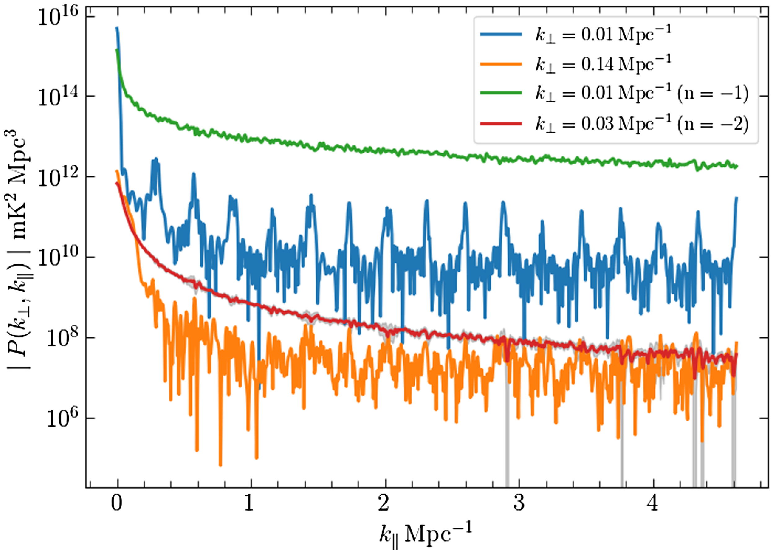
The results from our simulations suggests that the spikes and other artefacts seen in the measured $\mid P(k_{\perp}, k_{\parallel}) \mid$
presented here are not just a straightforward consequence of the periodic pattern of flagged channels. Our results seem to indicate that the spikes are possibly caused by some systematic effect in the data, which has the same period as the missing channels, periodic systematic errors in the calibration being one such possibility. We further note that it may be possible to model and remove these artefacts by subtracting out small period components from the measured
$\mid P(k_{\perp}, k_{\parallel}) \mid$
presented here are not just a straightforward consequence of the periodic pattern of flagged channels. Our results seem to indicate that the spikes are possibly caused by some systematic effect in the data, which has the same period as the missing channels, periodic systematic errors in the calibration being one such possibility. We further note that it may be possible to model and remove these artefacts by subtracting out small period components from the measured $C_{\ell}(\Delta\nu)$
using Gaussian process regression or some similar technique (Mertens et al. Reference Mertens, Ghosh and Koopmans2018; Elahi et al. Reference Elahi2023b).
$C_{\ell}(\Delta\nu)$
using Gaussian process regression or some similar technique (Mertens et al. Reference Mertens, Ghosh and Koopmans2018; Elahi et al. Reference Elahi2023b).
We next attempt to constrain the $z_c=8.2$
EoR 21-cm signal using the measured
$z_c=8.2$
EoR 21-cm signal using the measured $P(k_{\perp}, k_{\parallel})$
. To avoid significant foreground contamination, it is necessary to restrict the region of the
$P(k_{\perp}, k_{\parallel})$
. To avoid significant foreground contamination, it is necessary to restrict the region of the $(k_{\perp}, k_{\parallel})$
plane which is used to estimate the 21-cm signal. Here, we have limited the
$(k_{\perp}, k_{\parallel})$
plane which is used to estimate the 21-cm signal. Here, we have limited the $k_{\parallel} $
range to choose a region that is well above the foreground wedge. We further wish to avoid the large spikes seen in the measured
$k_{\parallel} $
range to choose a region that is well above the foreground wedge. We further wish to avoid the large spikes seen in the measured $\mid P(k_{\perp}, k_{\parallel}) \mid$
. We find that these spikes are relatively more prominent in the first six
$\mid P(k_{\perp}, k_{\parallel}) \mid$
. We find that these spikes are relatively more prominent in the first six $k_{\perp}$
bins where they extend over the entire
$k_{\perp}$
bins where they extend over the entire $k_{\parallel}$
range. In contrast, the spikes are not so prominent in the subsequent
$k_{\parallel}$
range. In contrast, the spikes are not so prominent in the subsequent $k_{\perp}$
bins where they also do not extend out to the large
$k_{\perp}$
bins where they also do not extend out to the large $k_{\parallel}$
range. This feature is visible when we compare the results for
$k_{\parallel}$
range. This feature is visible when we compare the results for $k_\perp = 0.01$
and
$k_\perp = 0.01$
and $0.14\,\mathrm{Mpc}^{-1}$
in Fig. 10. Based on the above considerations we have discarded the first six
$0.14\,\mathrm{Mpc}^{-1}$
in Fig. 10. Based on the above considerations we have discarded the first six $k_{\perp}$
bins and chosen the rectangular region
$k_{\perp}$
bins and chosen the rectangular region $0.05 \leq k_{\perp} \leq 0.16 \, \mathrm{Mpc^{-1}}$
and
$0.05 \leq k_{\perp} \leq 0.16 \, \mathrm{Mpc^{-1}}$
and $0.9 \leq k_{\parallel}\leq 4.6 \, \mathrm{Mpc^{-1}}$
, which is shown in the top right corner of the left panel of Fig. 9. The subsequent analysis is restricted to this rectangular region where
$0.9 \leq k_{\parallel}\leq 4.6 \, \mathrm{Mpc^{-1}}$
, which is shown in the top right corner of the left panel of Fig. 9. The subsequent analysis is restricted to this rectangular region where $\mid P(k_{\perp}, k_{\parallel}) \mid $
is found to have values in the range
$\mid P(k_{\perp}, k_{\parallel}) \mid $
is found to have values in the range $10^7$
–
$10^7$
– $10^{11} \, \mathrm{mK^2}\, \mathrm{Mpc^3}$
.
$10^{11} \, \mathrm{mK^2}\, \mathrm{Mpc^3}$
.
We now consider the statistics of the measured $P(k_{\perp}, k_{\parallel})$
, particularly to assess whether these values can be utilised to meaningfully constrain the EoR 21-cm signal. Following Pal et al. (Reference Pal, Bharadwaj, Ghosh and Choudhuri2021), we consider the quantity
$P(k_{\perp}, k_{\parallel})$
, particularly to assess whether these values can be utilised to meaningfully constrain the EoR 21-cm signal. Following Pal et al. (Reference Pal, Bharadwaj, Ghosh and Choudhuri2021), we consider the quantity
 \begin{equation} X=\frac{P(k_{\perp}, k_{\parallel})}{\unicode{x03B4} P_{N}(k_{\perp}, k_{\parallel})} \, \end{equation}
which is the ratio of the measured $P(k_{\perp}, k_{\parallel})$
to
$P(k_{\perp}, k_{\parallel})$
to $\unicode{x03B4} P_{N}(k_{\perp}, k_{\parallel})$
the statistical uncertainty expected from the system noise contribution only. We expect
$\unicode{x03B4} P_{N}(k_{\perp}, k_{\parallel})$
the statistical uncertainty expected from the system noise contribution only. We expect $X$
to have a symmetric distribution with mean
$X$
to have a symmetric distribution with mean $\mu = 0$
and standard deviation
$\mu = 0$
and standard deviation $\unicode{x03C3}_\mathrm{Est} = 1$
if the estimated values of
$\unicode{x03C3}_\mathrm{Est} = 1$
if the estimated values of $P(k_{\perp}, k_{\parallel})$
are consistent with the uncertainties predicted due to the system noise contribution only. Residual foreground contamination will manifest itself as a positive mean, whereas a negative mean would indicate some sort of negative systematics in the PS estimates. A value
$P(k_{\perp}, k_{\parallel})$
are consistent with the uncertainties predicted due to the system noise contribution only. Residual foreground contamination will manifest itself as a positive mean, whereas a negative mean would indicate some sort of negative systematics in the PS estimates. A value $\unicode{x03C3}_\mathrm{Est} > 1$
would indicate the presence of additional sources of uncertainty, beyond the predicted system noise contribution.
$\unicode{x03C3}_\mathrm{Est} > 1$
would indicate the presence of additional sources of uncertainty, beyond the predicted system noise contribution.
The middle panel of Fig. 9 shows the probability density function (PDF) of $X$
, which is found to be largely symmetric around 0 with
$X$
, which is found to be largely symmetric around 0 with $\mu=5.88 $
and
$\mu=5.88 $
and $\unicode{x03C3}_\mathrm{Est}=95.81 $
. Here, the substantially large value of
$\unicode{x03C3}_\mathrm{Est}=95.81 $
. Here, the substantially large value of $\unicode{x03C3}_\mathrm{Est}$
indicates that the measured
$\unicode{x03C3}_\mathrm{Est}$
indicates that the measured $P(k_{\perp}, k_{\parallel})$
has fluctuations which are considerably larger than those predicted from the system noise contribution alone. We note that several earlier works have reported such ‘excess variance’ for the estimated 21-cm PS at
$P(k_{\perp}, k_{\parallel})$
has fluctuations which are considerably larger than those predicted from the system noise contribution alone. We note that several earlier works have reported such ‘excess variance’ for the estimated 21-cm PS at $\sim$ $150 \, \mathrm{MHz}$
(Mertens et al. Reference Mertens2020; Pal et al. Reference Pal, Bharadwaj, Ghosh and Choudhuri2021) and also at higher frequencies
$150 \, \mathrm{MHz}$
(Mertens et al. Reference Mertens2020; Pal et al. Reference Pal, Bharadwaj, Ghosh and Choudhuri2021) and also at higher frequencies $ \sim$ $430 \, \mathrm{MHz} $
(Pal et al. Reference Pal2022; Elahi et al. Reference Elahi2023a,Reference Elahib, Reference Elahi2024). The exact cause of this excess variance is not known at present. We note that the earlier works which have applied the TGE (Pal et al. Reference Pal, Bharadwaj, Ghosh and Choudhuri2021, Reference Pal2022; Elahi et al. Reference Elahi2023a,Reference Elahib, Reference Elahi2024) have obtained values of
$430 \, \mathrm{MHz} $
(Pal et al. Reference Pal2022; Elahi et al. Reference Elahi2023a,Reference Elahib, Reference Elahi2024). The exact cause of this excess variance is not known at present. We note that the earlier works which have applied the TGE (Pal et al. Reference Pal, Bharadwaj, Ghosh and Choudhuri2021, Reference Pal2022; Elahi et al. Reference Elahi2023a,Reference Elahib, Reference Elahi2024) have obtained values of $\unicode{x03C3}_\mathrm{Est}$
in the range 2–5, whereas the value
$\unicode{x03C3}_\mathrm{Est}$
in the range 2–5, whereas the value $\unicode{x03C3}_\mathrm{Est}=95.81 $
obtained here is more than an order of magnitude larger. Although the exact cause is not known, it is plausible that the systematics responsible for the spikes in the PS at the lower values of
$\unicode{x03C3}_\mathrm{Est}=95.81 $
obtained here is more than an order of magnitude larger. Although the exact cause is not known, it is plausible that the systematics responsible for the spikes in the PS at the lower values of $k_{\perp}$
and
$k_{\perp}$
and $k_{\parallel}$
also causes excess fluctuations in
$k_{\parallel}$
also causes excess fluctuations in $P(k_{\perp}, k_{\parallel})$
within the rectangular region used to constrain the 21-cm signal. We find that the mean
$P(k_{\perp}, k_{\parallel})$
within the rectangular region used to constrain the 21-cm signal. We find that the mean $\mu=5.88 $
is not consistent with zero within the expected statistical fluctuations predicted using
$\mu=5.88 $
is not consistent with zero within the expected statistical fluctuations predicted using $\unicode{x03C3}_\mathrm{Est}$
. This indicates that the measured
$\unicode{x03C3}_\mathrm{Est}$
. This indicates that the measured $P(k_{\perp}, k_{\parallel})$
has some residual foreground contamination which introduces a positive bias in the distribution if
$P(k_{\perp}, k_{\parallel})$
has some residual foreground contamination which introduces a positive bias in the distribution if $X$
. We further note that the PDF of
$X$
. We further note that the PDF of $X$
is not Gaussian, and it nicely fit by a Lorentzian distribution with a peak location
$X$
is not Gaussian, and it nicely fit by a Lorentzian distribution with a peak location $x_0 = 1.68$
and spread
$x_0 = 1.68$
and spread $\gamma = 2.73$
, consistent with the earlier studies (Elahi et al. Reference Elahi2023a,Reference Elahib, Reference Elahi2024) all of which find that
$\gamma = 2.73$
, consistent with the earlier studies (Elahi et al. Reference Elahi2023a,Reference Elahib, Reference Elahi2024) all of which find that $X$
follows a Lorenztian distribution. For the subsequent analysis, we have scaled the system noise only error predictions with
$X$
follows a Lorenztian distribution. For the subsequent analysis, we have scaled the system noise only error predictions with $\unicode{x03C3}_\mathrm{Est}$
to account for the excess variance, that is, we have used
$\unicode{x03C3}_\mathrm{Est}$
to account for the excess variance, that is, we have used $ \unicode{x03B4} P(k_{\perp}, k_{\parallel}) = \unicode{x03C3}_\mathrm{Est} \times \unicode{x03B4} P_{N}(k_{\perp}, k_{\parallel}) $
to predict the statistical fluctuations expected in the measured
$ \unicode{x03B4} P(k_{\perp}, k_{\parallel}) = \unicode{x03C3}_\mathrm{Est} \times \unicode{x03B4} P_{N}(k_{\perp}, k_{\parallel}) $
to predict the statistical fluctuations expected in the measured $P(k_{\perp}, k_{\parallel})$
.
$P(k_{\perp}, k_{\parallel})$
.
We use the $(k_{\perp}, k_{\parallel})$
modes in the rectangular region mentioned earlier to estimate the spherical PS
$(k_{\perp}, k_{\parallel})$
modes in the rectangular region mentioned earlier to estimate the spherical PS $P(k)$
. The right panel of Fig. 9 shows the mean squared brightness temperature fluctuations
$P(k)$
. The right panel of Fig. 9 shows the mean squared brightness temperature fluctuations $\Delta^2(k) = k^3 P(k)/(2 \pi^2)$
as a function of
$\Delta^2(k) = k^3 P(k)/(2 \pi^2)$
as a function of $k$
along with the
$k$
along with the $2\unicode{x03C3}$
error bars corresponding to the predicted statistical fluctuations
$2\unicode{x03C3}$
error bars corresponding to the predicted statistical fluctuations $\unicode{x03B4} P(k_{\perp}, k_{\parallel})$
. The expected statistical fluctuations are much larger than the EoR 21-cm signal which is predicted to typically have values of the order of
$\unicode{x03B4} P(k_{\perp}, k_{\parallel})$
. The expected statistical fluctuations are much larger than the EoR 21-cm signal which is predicted to typically have values of the order of $\Delta^2(k) \sim 10^1-10^2 \, \mathrm{mK}^2 $
over the range
$\Delta^2(k) \sim 10^1-10^2 \, \mathrm{mK}^2 $
over the range $k=1 - 4 \, \mathrm{Mpc}^{-1} $
considered here (Mondal et al. Reference Mondal, Bharadwaj and Majumdar2017). In the absence of foreground contamination, we expect
$k=1 - 4 \, \mathrm{Mpc}^{-1} $
considered here (Mondal et al. Reference Mondal, Bharadwaj and Majumdar2017). In the absence of foreground contamination, we expect $\Delta^2(k)$
to fluctuate around 0 with both positive and negative values that are consistent with the predicted statistical fluctuations. We find that
$\Delta^2(k)$
to fluctuate around 0 with both positive and negative values that are consistent with the predicted statistical fluctuations. We find that $\Delta^2(k)$
in most of the
$\Delta^2(k)$
in most of the $k$
-bins are consistent with the statistical fluctuations, and the values are within
$k$
-bins are consistent with the statistical fluctuations, and the values are within $0\pm2\unicode{x03C3}$
. However, the values of
$0\pm2\unicode{x03C3}$
. However, the values of $\Delta^2(k)$
in the first, second, and sixth
$\Delta^2(k)$
in the first, second, and sixth $k$
-bins are somewhat larger, and these are consistent with the statistical fluctuations only at
$k$
-bins are somewhat larger, and these are consistent with the statistical fluctuations only at $0\pm5\unicode{x03C3}$
. It is possible that these
$0\pm5\unicode{x03C3}$
. It is possible that these $k$
-bin may have some residual foreground contamination, however, it is also possible that these are more extreme statistical fluctuations in the extended tail of the Lorentzian distribution. Note that the two
$k$
-bin may have some residual foreground contamination, however, it is also possible that these are more extreme statistical fluctuations in the extended tail of the Lorentzian distribution. Note that the two $k$
-bins with negative
$k$
-bins with negative $\Delta^2(k)$
values are both consistent with
$\Delta^2(k)$
values are both consistent with $0\pm2\unicode{x03C3}$
indicating that the estimated PS is free from any negative systematics. Since the measured PS is largely consistent with the statistical fluctuations and there are no negative systematics, we use the measured values to place
$0\pm2\unicode{x03C3}$
indicating that the estimated PS is free from any negative systematics. Since the measured PS is largely consistent with the statistical fluctuations and there are no negative systematics, we use the measured values to place $2\unicode{x03C3}$
upper limits on
$2\unicode{x03C3}$
upper limits on $\Delta^2(k)$
. The tightest upper limit is found to be
$\Delta^2(k)$
. The tightest upper limit is found to be $\Delta^2(k) \lt (1.85\times10^4)^2\, \mathrm{mK^2}$
at the first
$\Delta^2(k) \lt (1.85\times10^4)^2\, \mathrm{mK^2}$
at the first $k$
-bin
$k$
-bin $k=1 \,\mathrm{Mpc}^{-1}$
.
$k=1 \,\mathrm{Mpc}^{-1}$
.
6. Summary and discussion
Drift scan observations provide an economic and stable option with the broad sky coverage required for 21-cm EoR experiments. In this paper, we consider the TTGE (Reference Chatterjee, Bharadwaj, Choudhuri, Sethi and PatwaPaper I), which aims to measure the PS directly from the visibilities recorded in radio interferometric observations in the drift scan mode. The estimator is based on the TGE (Choudhuri et al. Reference Choudhuri2016) that has been widely used for analysing GMRT/uGMRT radio interferometric observations (Choudhuri et al. Reference Choudhuri2020; Pal et al. Reference Pal, Bharadwaj, Ghosh and Choudhuri2021, Reference Pal2022; Elahi et al. Reference Elahi2023a,Reference Elahib, Reference Elahi2024). The TGE works with gridded visibilities, a feature that makes it computationally efficient and also allows it to taper the sky response so as to suppress foreground contamination from the sources far away from the telescope’s pointing direction. While the original TGE was developed for observations where the telescope tracks a single field. The TTGE has been designed to work with drift scan observation. This estimator is tailored for observations with radio-interferometric arrays where the individual elements (antennas) are fixed on the ground (e.g. LOFAR, MWA, HERA, CHIME, upcoming SKA-low), and in the present work we have considered data from drift scan observations (Patwa et al. Reference Patwa, Sethi and Dwarakanath2021) with the compact configuration of MWA-II (Tingay et al. Reference Tingay2013). In drift scan observations, the sky moves across the telescope’s field of view with the passage of time. The TTGE allows us to follow a fixed position on the sky, namely the TC, as it moves across the telescope’s field of view. It further allows us to taper the sky response to a small angular region around the TC so as to suppress the foreground contamination from bright sources located at large angular separations from the TC.
In Reference Chatterjee, Bharadwaj, Choudhuri, Sethi and PatwaPaper I, we have presented the mathematical framework for the TTGE and validated this for a single-frequency channel. The analysis there considers an input model angular PS $C_{\ell}^M$
, for which the simulated sky signal and resulting drift scan visibilities are processed through the TTGE pipeline. The estimated
$C_{\ell}^M$
, for which the simulated sky signal and resulting drift scan visibilities are processed through the TTGE pipeline. The estimated $C_{\ell}$
is found to be in good agreement with
$C_{\ell}$
is found to be in good agreement with $C_{\ell}^M$
, thereby validating the TTGE. The present work validates the TTGE considering observations that cover multiple frequency channels spanning a finite bandwidth. Here, we have considered an input model PS
$C_{\ell}^M$
, thereby validating the TTGE. The present work validates the TTGE considering observations that cover multiple frequency channels spanning a finite bandwidth. Here, we have considered an input model PS $P^m(k)=(1 \mathrm{Mpc}^{-1}/k) \, \mathrm{K^2}\, \mathrm{Mpc^3}$
, for which simulated all-sky maps were used to calculate drift scan visibilities. These were processed through the TTGE pipeline to estimate the MAPS
$P^m(k)=(1 \mathrm{Mpc}^{-1}/k) \, \mathrm{K^2}\, \mathrm{Mpc^3}$
, for which simulated all-sky maps were used to calculate drift scan visibilities. These were processed through the TTGE pipeline to estimate the MAPS $C_{\ell}(\Delta\nu)$
which was found to be in good agreement with the predicted
$C_{\ell}(\Delta\nu)$
which was found to be in good agreement with the predicted $C_{\ell}^M(\Delta\nu)$
corresponding to
$C_{\ell}^M(\Delta\nu)$
corresponding to $P^{m}(k)$
(Fig. 3). We have used a MLE (Pal et al. Reference Pal2022; Elahi et al. Reference Elahi2023a) to directly compute both
$P^{m}(k)$
(Fig. 3). We have used a MLE (Pal et al. Reference Pal2022; Elahi et al. Reference Elahi2023a) to directly compute both $P(k_{\perp}, k_{\parallel})$
and
$P(k_{\perp}, k_{\parallel})$
and $P(k)$
from the estimated
$P(k)$
from the estimated $C_{\ell}(\Delta\nu)$
. The estimated
$C_{\ell}(\Delta\nu)$
. The estimated $P(k)$
is found to be in good agreement with the input model
$P(k)$
is found to be in good agreement with the input model $P^{m}(k)$
(Fig. 5), thereby validating the TTGE for 3D multi-frequency data.
$P^{m}(k)$
(Fig. 5), thereby validating the TTGE for 3D multi-frequency data.
The MWA has a periodic pattern of flagged channels, the period being $\Delta\nu_\mathrm{per} = 1.28 \,\mathrm{MHz}$
(Fig. 2). In addition, there is the possibility of other frequency channels also being flagged in order to avoid manmade RFI, etc. Several earlier works which have first transformed from frequency to delay space and then estimated the PS (e.g. Paul et al. Reference Paul2016; Li et al. Reference Li2019; Trott et al. Reference Trott2020; Patwa et al. Reference Patwa, Sethi and Dwarakanath2021) have reported a very prominent pattern of horizontal streaks in the estimated
$\Delta\nu_\mathrm{per} = 1.28 \,\mathrm{MHz}$
(Fig. 2). In addition, there is the possibility of other frequency channels also being flagged in order to avoid manmade RFI, etc. Several earlier works which have first transformed from frequency to delay space and then estimated the PS (e.g. Paul et al. Reference Paul2016; Li et al. Reference Li2019; Trott et al. Reference Trott2020; Patwa et al. Reference Patwa, Sethi and Dwarakanath2021) have reported a very prominent pattern of horizontal streaks in the estimated $P(k_{\perp}, k_{\parallel})$
due to the periodic pattern of flagged channels present in the MWA data. In our approach approach (Bharadwaj et al. Reference Bharadwaj, Pal, Choudhuri and Dutta2018), we first estimate
$P(k_{\perp}, k_{\parallel})$
due to the periodic pattern of flagged channels present in the MWA data. In our approach approach (Bharadwaj et al. Reference Bharadwaj, Pal, Choudhuri and Dutta2018), we first estimate $C_{\ell}(\Delta\nu)$
, which does not have any missing
$C_{\ell}(\Delta\nu)$
, which does not have any missing $\Delta\nu$
even when the visibility data contains flagged channels. We then Fourier transform
$\Delta\nu$
even when the visibility data contains flagged channels. We then Fourier transform $C_{\ell}(\Delta\nu)$
to obtain a clean estimate of
$C_{\ell}(\Delta\nu)$
to obtain a clean estimate of $P(k_{\perp}, k_{\parallel})$
. Considering the simulated data, we see that the missing frequency channels do not introduce any artefacts in the estimated
$P(k_{\perp}, k_{\parallel})$
. Considering the simulated data, we see that the missing frequency channels do not introduce any artefacts in the estimated $P(k_{\perp}, k_{\parallel})$
(Fig. 4). We find that the estimated
$P(k_{\perp}, k_{\parallel})$
(Fig. 4). We find that the estimated $P(k_{\perp}, k_{\parallel})$
are visually indistinguishable irrespective of whether there are flagged channels or not. We conclude that our estimator is impervious to the periodic pattern of flagged channels, and these do not introduce any artefacts in the estimated
$P(k_{\perp}, k_{\parallel})$
are visually indistinguishable irrespective of whether there are flagged channels or not. We conclude that our estimator is impervious to the periodic pattern of flagged channels, and these do not introduce any artefacts in the estimated $P(k_{\perp}, k_{\parallel})$
.
$P(k_{\perp}, k_{\parallel})$
.
We have applied the TTGE to estimate the PS for a single pointing of the actual MWA data, which effectively corresponds to using the TGE. The pointing centre PC=34 corresponds to $(\mathrm{RA,DEC)} = (6.1^{\circ},-26.7^{\circ})$
(Fig. 1) with an observing time of approximately
$(\mathrm{RA,DEC)} = (6.1^{\circ},-26.7^{\circ})$
(Fig. 1) with an observing time of approximately $17 \, \mathrm{min}$
. For the tapering, we have used a Gaussian window function with
$17 \, \mathrm{min}$
. For the tapering, we have used a Gaussian window function with $\unicode{x03B8}_\mathrm{FWHM} = 15^{\circ}$
. The estimated MAPS
$\unicode{x03B8}_\mathrm{FWHM} = 15^{\circ}$
. The estimated MAPS $C_{\ell} (\Delta \nu)$
, arising mainly from foregrounds, is shown in Fig. A1. This does not appear to exhibit any prominent features which can be associated with the periodic pattern of flagged channels. However, on fitting and subtracting out a smooth polynomial in
$C_{\ell} (\Delta \nu)$
, arising mainly from foregrounds, is shown in Fig. A1. This does not appear to exhibit any prominent features which can be associated with the periodic pattern of flagged channels. However, on fitting and subtracting out a smooth polynomial in $\Delta \nu$
, for several
$\Delta \nu$
, for several $\ell$
values the residual
$\ell$
values the residual $C_{\ell}(\Delta \nu)$
exhibit oscillations of period
$C_{\ell}(\Delta \nu)$
exhibit oscillations of period $\Delta \nu_\mathrm{per}=1.28 \, \mathrm{MHz}$
. The amplitude of these oscillating residuals is approximately two orders of magnitude smaller than the total
$\Delta \nu_\mathrm{per}=1.28 \, \mathrm{MHz}$
. The amplitude of these oscillating residuals is approximately two orders of magnitude smaller than the total $C_{\ell}(\Delta \nu)$
. The left panel of Fig. 9 shows the cylindrical PS
$C_{\ell}(\Delta \nu)$
. The left panel of Fig. 9 shows the cylindrical PS $P(k_{\perp}, k_{\parallel})$
estimated from the measured
$P(k_{\perp}, k_{\parallel})$
estimated from the measured $C_{\ell}(\Delta \nu)$
. We find that the foregrounds are mainly localised within the expected foreground wedge boundary, with some leakage beyond. We notice a few horizontal streaks in the PS that extend across several
$C_{\ell}(\Delta \nu)$
. We find that the foregrounds are mainly localised within the expected foreground wedge boundary, with some leakage beyond. We notice a few horizontal streaks in the PS that extend across several $k_{\perp}$
bins at some fixed
$k_{\perp}$
bins at some fixed $k_{\parallel}$
values.
$k_{\parallel}$
values.
To understand the origin of these streaks, we consider Fig. 10 where we find the PS at $k_\perp=0.01\,\mathrm{Mpc}^{-1}$
shows spikes at a regular interval of
$k_\perp=0.01\,\mathrm{Mpc}^{-1}$
shows spikes at a regular interval of $\Delta k_{\parallel}\sim 0.29\,\mathrm{Mpc}^{-1}$
which matches
$\Delta k_{\parallel}\sim 0.29\,\mathrm{Mpc}^{-1}$
which matches $\Delta \nu_\mathrm{per}=1.28 \, \mathrm{MHz}$
in
$\Delta \nu_\mathrm{per}=1.28 \, \mathrm{MHz}$
in $C_{\ell}(\Delta \nu)$
. We attribute the spike in
$C_{\ell}(\Delta \nu)$
. We attribute the spike in $P(k_{\perp}, k_{\parallel})$
to the periodic oscillation in
$P(k_{\perp}, k_{\parallel})$
to the periodic oscillation in $C_{\ell}(\Delta \nu)$
. We also find that
$C_{\ell}(\Delta \nu)$
. We also find that $P(k_{\perp}, k_{\parallel})$
does not exhibit such prominent spikes at the larger
$P(k_{\perp}, k_{\parallel})$
does not exhibit such prominent spikes at the larger $k_{\perp}$
bins. Further, such spikes are also not present in the
$k_{\perp}$
bins. Further, such spikes are also not present in the $P(k_{\perp}, k_{\parallel})$
estimated from simulations, which incorporate the periodic pattern of flagged channels. Note, however, that the dynamic range of the present simulations is an order of magnitude lower than the actual data. In future work, we plan to carry out foreground simulations where we expect to achieve a higher dynamic range.
$P(k_{\perp}, k_{\parallel})$
estimated from simulations, which incorporate the periodic pattern of flagged channels. Note, however, that the dynamic range of the present simulations is an order of magnitude lower than the actual data. In future work, we plan to carry out foreground simulations where we expect to achieve a higher dynamic range.
The origin of the small periodic oscillation in $C_{\ell}(\Delta\nu)$
, which is responsible for the spikes in
$C_{\ell}(\Delta\nu)$
, which is responsible for the spikes in $P(k_{\perp}, k_{\parallel})$
, is not known at present. The fact that these features are not present in the simulations suggests that our estimator is impervious to the periodic pattern of flagged channels, and the spikes are not just a straightforward consequence of the missing channels. Our results seem to indicate that the spikes are possibly caused by some systematic effect in the data, which has the same period as the missing channels, periodic systematic errors in the calibration being one such possibility. We note that the streaks found here are an order of magnitude smaller than those found in earlier analyses of MWA data (e.g. Patwa et al. Reference Patwa, Sethi and Dwarakanath2021). It may be possible to model and remove these artefacts by subtracting out small period components from the measured
$P(k_{\perp}, k_{\parallel})$
, is not known at present. The fact that these features are not present in the simulations suggests that our estimator is impervious to the periodic pattern of flagged channels, and the spikes are not just a straightforward consequence of the missing channels. Our results seem to indicate that the spikes are possibly caused by some systematic effect in the data, which has the same period as the missing channels, periodic systematic errors in the calibration being one such possibility. We note that the streaks found here are an order of magnitude smaller than those found in earlier analyses of MWA data (e.g. Patwa et al. Reference Patwa, Sethi and Dwarakanath2021). It may be possible to model and remove these artefacts by subtracting out small period components from the measured $C_{\ell}(\Delta\nu)$
using Gaussian process regression or some similar technique (Mertens et al. Reference Mertens, Ghosh and Koopmans2018; Elahi et al. Reference Elahi2023b). We plan to address this in future work.
$C_{\ell}(\Delta\nu)$
using Gaussian process regression or some similar technique (Mertens et al. Reference Mertens, Ghosh and Koopmans2018; Elahi et al. Reference Elahi2023b). We plan to address this in future work.
We identify a rectangular region $0.05 \leq k_{\perp} \leq 0.16 \, \mathrm{Mpc^{-1}}$
and
$0.05 \leq k_{\perp} \leq 0.16 \, \mathrm{Mpc^{-1}}$
and $0.9 \leq k_{\parallel}\leq 4.6 \, \mathrm{Mpc^{-1}}$
to be relatively free of foreground contamination, spikes, and other artefacts. We use the
$0.9 \leq k_{\parallel}\leq 4.6 \, \mathrm{Mpc^{-1}}$
to be relatively free of foreground contamination, spikes, and other artefacts. We use the $P(k_{\perp}, k_{\parallel})$
estimates in this region to constrain the EoR 21-cm signal. The
$P(k_{\perp}, k_{\parallel})$
estimates in this region to constrain the EoR 21-cm signal. The $P(k_{\perp}, k_{\parallel})$
values, suitably scaled with the uncertainties expected from the system noise, are found to be nearly symmetrically distributed around 0. The distribution is well-fitted with a Lorentzian profile. However, the standard deviation is roughly 100 times of that expected from the contribution from system noise alone. The cause of this excess variance is not known. We have used our measurements to place a
$P(k_{\perp}, k_{\parallel})$
values, suitably scaled with the uncertainties expected from the system noise, are found to be nearly symmetrically distributed around 0. The distribution is well-fitted with a Lorentzian profile. However, the standard deviation is roughly 100 times of that expected from the contribution from system noise alone. The cause of this excess variance is not known. We have used our measurements to place a $2\unicode{x03C3}$
upper limit
$2\unicode{x03C3}$
upper limit $\Delta^2(k) \lt (1.85\times10^4)^2\, \mathrm{mK^2}$
on the mean squared 21-cm brightness temperature fluctuations at
$\Delta^2(k) \lt (1.85\times10^4)^2\, \mathrm{mK^2}$
on the mean squared 21-cm brightness temperature fluctuations at $k=1 \,\mathrm{Mpc}^{-1}$
. The present results, which are restricted to a single pointing, are limited by foregrounds and the systematics whose origins are not known to us at present. It is necessary to address these issues before combining multiple pointings. We plan to address these issues in future work.
$k=1 \,\mathrm{Mpc}^{-1}$
. The present results, which are restricted to a single pointing, are limited by foregrounds and the systematics whose origins are not known to us at present. It is necessary to address these issues before combining multiple pointings. We plan to address these issues in future work.
Acknowledgements
S. Chatterjee acknowledges support from the South African National Research Foundation (Grant No. 84156) and the Department of Atomic Energy, Government of India, under project no. 12-R & D-TFR-5.02-0700. S. Chatterjee would also like to thank Dr. Devojyoti Kansabanik, for helpful discussions.
Data availability
The data sets were derived from sources in the public domain (the MWA Data Archive: project ID G0031) at https://asvo.mwatelescope.org/.
Appendix 1. Preliminary results: MAPS
We have applied the TTGE on MWA drift scan observation to estimate the MAPS $C_{\ell}(\Delta\nu)$
(Section 5). Fig. A1 shows
$C_{\ell}(\Delta\nu)$
(Section 5). Fig. A1 shows $C_{\ell}(\Delta\nu)$
for different
$C_{\ell}(\Delta\nu)$
for different $\ell$
whose values are annotated in each panel. The estimated
$\ell$
whose values are annotated in each panel. The estimated $C_{\ell}(\Delta\nu)$
have values
$C_{\ell}(\Delta\nu)$
have values $\sim$ $2\times10^5 \,\mathrm{mK}^2$
at
$2\times10^5 \,\mathrm{mK}^2$
at $\Delta\nu=0$
, and it gradually decreases with increasing
$\Delta\nu=0$
, and it gradually decreases with increasing $\Delta\nu$
. This gradual decorrelation is a typical behaviour of foregrounds, which has a smooth frequency dependence. Further, the decorrelation becomes faster with increasing
$\Delta\nu$
. This gradual decorrelation is a typical behaviour of foregrounds, which has a smooth frequency dependence. Further, the decorrelation becomes faster with increasing $\ell$
due to baseline migration (Pal et al. Reference Pal2022). We note that point sources, which are in the sidelobes of the telescopes, introduce oscillatory features in
$\ell$
due to baseline migration (Pal et al. Reference Pal2022). We note that point sources, which are in the sidelobes of the telescopes, introduce oscillatory features in $C_{\ell}(\Delta\nu)$
, which are not prominent in these plots. This is because the contribution from the sources within the field of view of the PB is much larger than those appearing through the sidelobes. We plan to identify and remove the point sources that are in the field of view of the PB in future work.
$C_{\ell}(\Delta\nu)$
, which are not prominent in these plots. This is because the contribution from the sources within the field of view of the PB is much larger than those appearing through the sidelobes. We plan to identify and remove the point sources that are in the field of view of the PB in future work.
This figure shows $C_{\ell}(\Delta\nu)$
for the annotated
$C_{\ell}(\Delta\nu)$
for the annotated $\ell$
values. The blue dashed curves show a polynomial fit on the range
$\ell$
values. The blue dashed curves show a polynomial fit on the range $\Delta\nu<6$
MHz. The polynomial fit is subtracted from the measured
$\Delta\nu<6$
MHz. The polynomial fit is subtracted from the measured $C_{\ell}(\Delta\nu)$
, and the residual
$C_{\ell}(\Delta\nu)$
, and the residual $C_{\ell}(\Delta\nu)$
are shown in the insets (red).
$C_{\ell}(\Delta\nu)$
are shown in the insets (red).
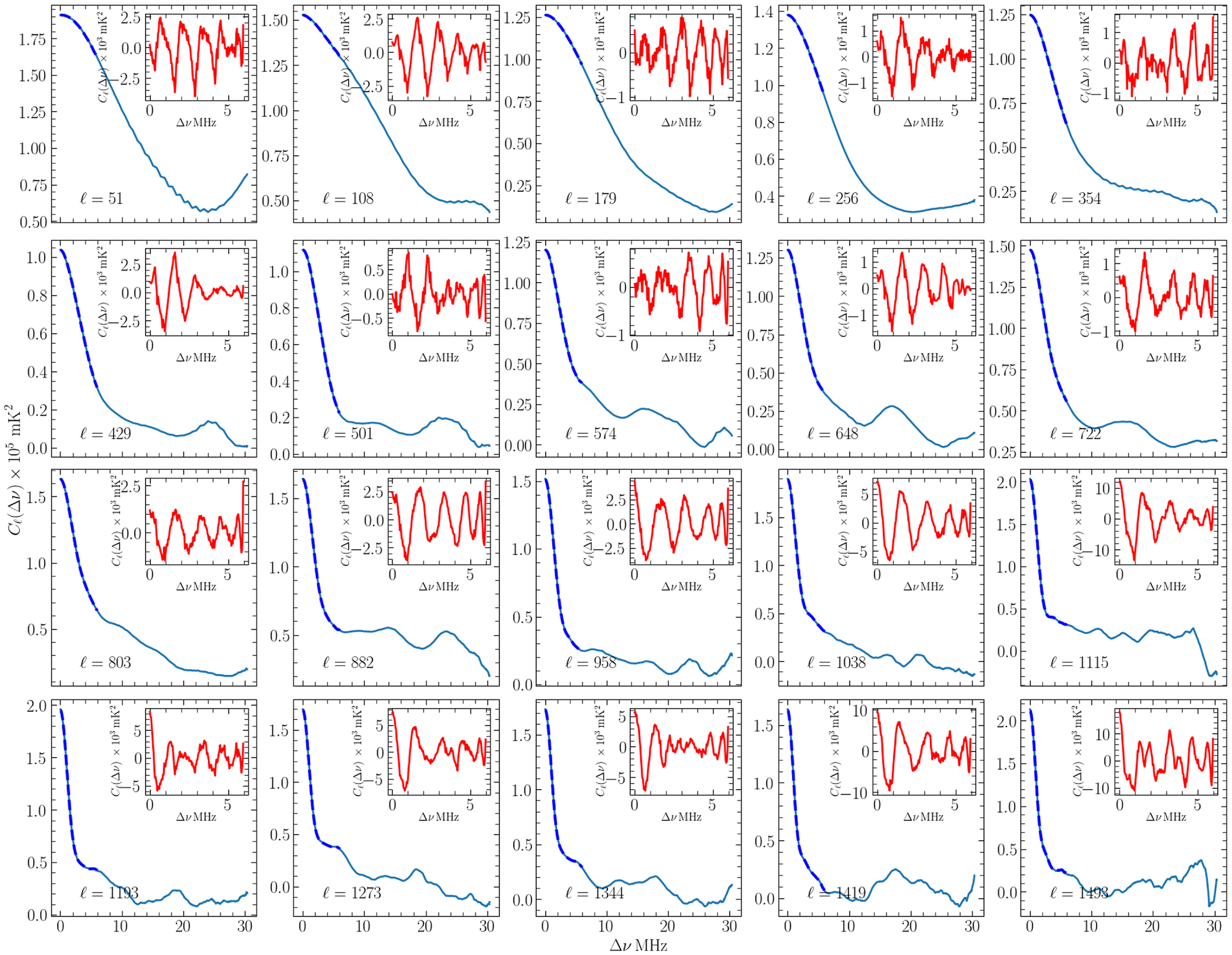
We see no prominent features in the estimated $C_{\ell}(\Delta\nu)$
but find features in the PS (Fig. 9), which leads us to investigate the measured
$C_{\ell}(\Delta\nu)$
but find features in the PS (Fig. 9), which leads us to investigate the measured $C_{\ell}(\Delta\nu)$
closely. The idea is to fit the measured
$C_{\ell}(\Delta\nu)$
closely. The idea is to fit the measured $C_{\ell}(\Delta\nu)$
with a polynomial and subtract the polynomial fit to look for any features in the residual
$C_{\ell}(\Delta\nu)$
with a polynomial and subtract the polynomial fit to look for any features in the residual $C_{\ell}(\Delta\nu)$
. Here we have chosen the range
$C_{\ell}(\Delta\nu)$
. Here we have chosen the range $\Delta\nu<6$
MHz and fitted the estimated
$\Delta\nu<6$
MHz and fitted the estimated $C_{\ell}(\Delta\nu)$
with an even polynomial having 10 terms. The blue dashed curves on top of the measured
$C_{\ell}(\Delta\nu)$
with an even polynomial having 10 terms. The blue dashed curves on top of the measured $C_{\ell}(\Delta\nu)$
show the polynomial fits, and the residual
$C_{\ell}(\Delta\nu)$
show the polynomial fits, and the residual $C_{\ell}(\Delta\nu)$
are shown in the insets (red).
$C_{\ell}(\Delta\nu)$
are shown in the insets (red).


 Open access