Introduction

The most prominent event of the deglaciation of Scandinavia occurred during the period called the Younger Dryas (11000–10200BP). Previous studies of the Younger Dryas have underestimated and often neglected glaciological problems. A reasonable scenario for the simulation of the Younger Dryas should be able to account for its different responses in different areas of Scandinavia. In an effort to develop a scenario that would produce the Younger Dryas event in central Scandinavia, the response of the ice sheet to changing climatic conditions was simulated using a finite-element map-plane model.

The climatic boundary between the previous warmer Alleröd and cooler Younger Dryas is abrupt, with a sudden drop in temperature of several degrees. The largest changes are on the British Isles and in Norway, declining to the east. Some now argue that the Younger Dryas was a worldwide event (Reference Broecker and DentonBroecker and Denton, 1989, Reference Broecker and Denton1990; Reference Kudrass, Erlenkeuser, Vollbrecht and WeissKudrass and others, 1991) with manifestations in North and South America and in the Sulu Sea.

In eastern Sweden, the scenario seems to be fairly clear. The ice front receded slowly all through the Younger Dryas period, leaving no sign of re-advance or long-term stillstand (Reference KristianssonKristiansson, 1986). In Finland, there are three large moraines (Salpaussälkä) associated with the Younger Dryas though the climatic signal is similar to what has been recorded elsewhere in Scandinavia (Reference DonnerDonner, 1978). The deglaciation after 10 000 BP has been described in detail by Reference Ignatius, Korpela and KujansuuIgnatius and others (1980).

The Younger Dryas event in Scandinavia has distinctly different responses in different regions. Along the west coast of Norway and in southwestern Sweden, a distinct re-advance of the margin occurs during the Younger Dryas event, whereas in eastern Sweden, central Sweden and Finland only a brief stillstand, or pause in the retreat, is observed. Following this stillstand, the margin retreated rapidly into the western mountains, with full deglaciation occurring in just over 1000 years. Retreat was less rapid from the west, with the final ice cap residing over the high western mountains.

Presumably, this distinction is due to the differing climatic regimes dominating the two areas. In the west, a more maritime regime dominates, with higher accumulation and ablation rates, and flow is channeled more into outlet glaciers. In the eastern zone, the climatic regime is more continental with more moderate accumulation and ablation rates, and the terrain is more uniform.

We are concerned primarily with the response in this continental climatic zone. Here, the topography is relatively flat, so that the effects of channelized flow apparent in the outlet glaciers of the western zone are not as pronounced. Response of the ice-sheet margin presumably reflects the larger processes that impact the ice sheets, whereas in the west, localized precipitation changes will dominate the ice-sheet response.

The Finite-Element Solution

The model consists of a finite-element solution of the two-dimensional (map-plane) time-dependent mass-continuity equation, given by the following expression:

. (1)

The accumulation rate, ȧ, represents the net total of both the snowfall rate and the melting rate at a point (x, y) of the domain.

To complete this equation, one must relate the flux, σ, to the ice-surface elevation, h, through a constitutive equation. For non-Newtonian fluids such as ice, this involves a non-linear relationship that depends on the ice-surface elevation, the thickness and the surface slope. We can, however, linearize this by absorbing all dependencies on h and all non-linearities in the surface slope into a spatial non-uniform time-dependent proportionality constant, k(x, y). This constitutive equation relating ice flux to surface slope can be expressed by

(2)

where U is the column-averaged velocity and H is the thickness of the ice column.

The material coefficient k(x, y) is dependent upon the form of the flow and sliding laws. We use Glen’s flow law (Reference GlenGlen, 1955) for the component of velocity due to internal deformation of the ice, given by the following expression:

. (3)

The flow parameter, A, represents a column-averaged ice hardness which is obtained by calibrating the model with existing ice sheets, primarily in Antarctica (Reference Fastook, Billingley, Brown and DerohanesFastook, 1992; Reference Fastook and PrenticeFastook and Prentice, 1994) It should be pointed out that this model does not include a thermodynamic solution, so that temperatures are not included or dealt with explicitly. However, warmer temperatures would result in a smaller ice-hardness parameter reflecting the softening of the ice as it approaches the melting point.

The sliding law used here is a general relationship for beds at the melting point developed by (Reference WeertmanWeertman 1957, Reference Weertman1964) and given by the following expression:

. (4)

The relationship is a simplified parameterization of the sliding process which does not account for variation in basal-water pressure or deformable sediments, but is representative of the sliding process whereby high velocities result from relatively lower surface slopes.

The column-averaged ice velocity for a combination of these two modes of motion is

(5)

where f is the fraction of velocity due to sliding. For existing ice sheets, f can be used as a parameter to “tune” the model. For reconstructing ice sheets from the past and for extrapolating future behavior, f can be estimated from various erosional features found in the glacial geologic record (Reference Hughes, Denton and HughesHughes, 1980).

The form of k(x, y) is obtained by combining Equation (3), (4) and (5) and substituting into Equation (2).

. (6)

This shows the dependence of the material coefficient on ice density, gravity, flow-law constant and sliding-law constant (both of which are dependent on ice temperature, ice-crystal size, impurity content, etc.) and surface gradient.

The surface elevation, h, and the ice thickness, H, are related through the bedrock elevation, which is modified to account for isostatic depression by the ice load. Bed depression is calculated for a point load at each grid location from a hydrostatic loading condition. Delayed rebound is not accounted for, and the bed is at all times in hydrostatic equilibrium.

Substituting the constitutive-law expression for σ(x, у) from Equation (2) into continuity Equation (1) yields the following differential equation in h:

. (7)

The presence of k(x,y) in the continuity equation incorporates the physics of the flow and sliding laws into the problem, since its form depends on the form of the flow and sliding law. Different treatments of the flow and sliding process change the form of k(x, y) but do not affect the method with which the problem is solved. An entirely different sliding relationship can be substituted without materially affecting the method of solving this equation.

The solution is obtained by first assuming a value for k(х, y) over the domain of the problem, and solving Equation (7) for h. With this solution for the surface elevation and ice thickness, a new k(x,y) is obtained from Equation (6). This iterative process is repeated a handful of times until the solution is self-consistent.

The finite-element method assumes linear spatial interpolants for the solution of this differential equation, turning the problem into a set of algebraic equations which can be solved by ordinary matrix methods. The output of such a solution consists of ice-surface elevations and thicknesses at each of the two-dimensional grid points, as a function of time.

Boundary Conditions for Scandinavia

Our grid for Scandinavia is obtained from an electronic map of the world’s surface which has bedrock topography at 5 min intervals both in latitude and longitude (Anonymous, 1988). A reduced data set with 1492 nodal points and 1403 quadrilateral elements is obtained by using the nearest data point from the map. The grid spacing is variable but is roughly 50 km in the north–south direction and 10 km in the east-west direction. The sliding fraction is 0 everywhere the present bed is higher than 100 m above present sea level. The flow-law parameter is 2.0 m^1/3 and the sliding-law parameter is 0.02 bar m^1/2. The flow parameter is obtained by assuming an average ice temperature of about −10°C, using an empirical relation stated by Reference HookeHooke (1981).

For this experiment, we begin with a maximum configuration ice sheet that has not quite attained steady-state equilibrium. This ice sheet is generated from an ice-free bed in roughly 35 000 years using a mass-balance scheme typical of polar continental regions for the entire ice sheet. Figure 1 shows the volume as a function of time for this growth phase of the model. Note that full equilibrium is attained for such a growing ice sheet in approximately 50 000 years. Figure 2 shows the surface-elevation contours for this non-equilibrium ice sheet at its maximum extent.

Fig. 1. The growth of the Weichselian ice sheet according to this model.

Fig. 2. The Scandinavian ice sheet at about 15000 BP. The contours indicate each 500 m height interval.

In this mass-balance regime, the accumulation rate is a function of elevation only and is given by the relationship

(8)

where A ₁ = −1.30, L ₁ = 1.50 × 10⁻⁵, A ₂ = 0.30 and L ₂ = 3.66 × 10⁻⁸. These values were obtained from a least-squares fit to available data for analogous present climatic zones (Reference Pelto, Higgins, Hughes and FastookPelto and others, 1990). ΔS _N allows us to vary the equilibrium-line elevation without changing the shape of the overall mass-balance curve. With ΔS _N = 0, this mass-balance relationship has an equilibrium-line elevation at 310 m, an ablation rate at sea level of −1 m year⁻¹ ice equivalent, and a peak accumulation rate of 0.29 m year⁻¹ at an elevation of 710 m, declining to a polar desert value of 0.16 m year⁻¹ at 4000 m.

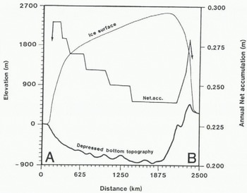
Figure 3 shows a transect depicting surface elevations, bed elevations and net accumulation rates along a line from point A near Denmark to point B in northern Norway. This transect follows along the trough of the “Baltic Ice Stream” and across the ice divide to the margin along the Norwegian continental shelf.

Fig. 3. The net accumulation, the surface level and the bottom topography along the profile A–B indicated in Figure 2.

Assumptions for the basal conditions are based on geologic evidence and hypsographic information from the Baltic Sea and the Gulf of Bothnia. The general assumption is that the bed was frozen on all bed elevations above today’s 100 m level. Between this level and −100 m, the glacier is assumed to slide in accordance with the relation suggested by (Reference WeertmanWeertman 1957, Reference Weertman1964). Where the bed is below −100 m, we used a softer sliding constant of half the value used in the −100 to 100 m zone. This distribution of basal zones is shown in Figure 4. This enhanced rate was added to simulate deformable sediments. On the island Aland, however, the ice was assumed to be frozen to its bed. This was done in order to provide an obstacle for the flow from the Gulf of Bothnia out into the Baltic Sea, thereby preventing the formation of multiple domes during the deglaciation.

Fig. 4. Basal conditions used in the model.

These assumptions are reasonable as it is likely that the bottom of the Baltic Sea and the Gulf of Bothnia was at the pressure-melting point throughout most of the glaciation. The Baltic Sea may have been frozen to its bed during some initial phase of the glaciation, but it would have thawed as the ice sheet thickened. These conditions coincide with the concept of an ice sheet drained by a “Baltic Ice Stream” (Reference TorellTorell, 1873; Reference Boulton, Smith, Jones and NewsomeBoulton and others, 1985; Reference LundqvistLundquist, 1987). The fact that flow turned to the west in the southern part of the Baltic Sea was probably due to more favorable basal conditions and higher melt rates towards the west.

When the model enters the warmer post-glacial climate phase, the low profile of the Baltic Ice Stream results in high ablation rates and the ice melts off quickly up to Åland Island. Although Gotland and Öland Islands do not seem to have been major obstacles for the ice flow, Åland Island must have been an important obstacle. Otherwise, as the model shows, if the ice there is not frozen to the bed, the ice sheet drains too quickly, leaving one major dome in Sweden and a minor one in Finland, a pattern inconsistent with observation.

We can only estimate how long this frozen zone existed over Åland Island, since our model does not explicitly model the thermodynamics. The frozen bed may be an effect of the thinning of the ice sheet. It is possible that the bed around Åland Island was at the pressure-melting point during most of the glaciation except for the very last few thousand years. The extent to which the bed was frozen during the Younger Dryas determines the position of the margin during the same period.

When the warm climate was re-established after the termination of the Younger Dryas event, the profile of the ice sheet was low, producing higher recession rates (Figs 5 and 6; Tables 1 and 2). As the region around Åland Island became ice-free, the ice stream from the Gulf of Bothnia was re-activated and the interior of the remaining ice sheet drained quickly.

Fig. 5. The modeled scenario showing the snow line and the volume and area of the ice sheet.

Fig. 6. The recession of the Scandinavian ice sheet in 1000 year steps between 15000 and 8000 BP.

Table 1. Modeled scenario (Fig. 5)

Table 2. Basal conditions (Fig. 4)

Model sensitivity

To test the suggested scenario in this paper, we made some model runs with extreme conditions. These test runs began with a configuration close to the maximum extent of the Weichselian ice sheet. In all of these experiments the climatic signal was a sudden 1200 m change of the equilibrium line from 300 to 1500 m. In the first experiment, the bed was allowed to be thawed over the entire region. In the second experiment, the bed was frozen over the entire region. The third experiment compared two retreat scenarios that differ only in the mechanical hardness of the ice, which was decreased in an attempt to simulate stillstand.

In the first experiment, when the whole ice sheet suddenly became wet-based with no frozen spots, the ice sheet collapsed and had gone after only 2400 years (Fig. 7a). The last remnants of the ice occurred in the Gulf of Bothnia.

Fig. 7. Volume and area of the ice sheet as a function of time.

In the second experiment, with the ice frozen everywhere to its bed, the glacier attained a new state of equilibrium after about 1000 years (Fig. 7). After 400 years, its areal extent was smaller than at the maximum, but it was almost 1000 m thicker in the center, despite the warmer climate. This ice sheet would probably not have disappeared even during the warmest parts of the Holocene.

These two scenarios suggest that the bed had to be a mixture of frozen and thawed zones. With no sliding, the profile was too high for the expected snow-line lowering to remove the ice sheet, while with all sliding the profile was so low that recession and collapse of the ice sheet proceeded too rapidly. These considerations led to the simple scheme of allowing sliding below 100 m bedrock elevation. Places where the bed was lowest would generally coincide with areas where the ice was thickest, and hence most likely to be at the pressure-melting point. For higher elevations, we expect that the thinner ice overburden would allow more of the heat to escape so that the bed was frozen and no sliding could occur.

The final test concerned the relative importance of the external climatic signal and internal dynamic changes within the ice during the Younger Dryas. In the first part of this test, we just excluded the cold period described in Table 1. We used the basal conditions described earlier (a simple mix of frozen and thawed bed based on bedrock elevation) with the same climate scenario as in the first two experiments. With this simple scenario, the decline in volume was quite uniform for the first 4000 years of retreat, after which the rate declined slightly. The ice vanished completely in another 4000 years. This is the solid line о in Figure 7b. The areal extent for this scenario is indicated by the dashed line, which merges with the volume curve after 11 000 years. Since there is no climatic cooling, there is no stillstand in this scenario. Note that 90% of the initial volume is removed in this first 4000 years, while only about 60% of the area is removed. The reduction in the recession rate and the mass loss are probably due to the frozen ground in the interior of northern Sweden. As this scenario did not produce a prominent stillstand at the Younger Dryas period, and since other evidence indicates that a definite cooler period did occur, we only include this model for comparison with the next part of this experiment.

In the second part of this experiment, we also excluded the climatic signal but added a softening factor to the remaining ice after 4000 years. As a result, the recession rate (indicated by the area extent, the dashed curve b in Figure 7b) decreases during the Younger Dryas while the mass loss (indicated by the volume, the solid curve b in Figure 7b) continues and accelerates all through the period. This is due to lowering of the ice-sheet interior because of the reduced bed coupling. This produces a higher flux of ice at the margin which temporarily overwhelms the ablation, producing a still-stand of the margin. This decoupling causes the ice to disappear a few thousand years earlier than it did in the scenario without softening (Fig. 7b b). This result is important as it shows a reduction of the recession speed without a climatic signal.

Caution is in order in interpreting a re-advance of the margin as an indicator of climatic cooling, since it may be due to a change in mechanical properties. If the stillstand is brief, and the ensuing retreat is rapid, it is possible that such an event could be caused by abrupt reduction in bed coupling. However, as the climatic signal is well documented we do not feel that this is the mechanism that produced the Younger Dryas.

Discussion

Modeling results require relatively thin ice following the Younger Dryas event in order for the ice to disappear in the following 1000 years or so. The low ice-surface elevation required for this rapid retreat could only be obtained if much of the Baltic Sea region had a basal sliding condition. In addition, this allows only a relatively brief climatic deterioration which does not produce significant thickening during the Younger Dryas period. The presence of an obstacle to flow near Åland Island arises from the need to slow this thinning during deglaciation prior to the Younger Dryas period. The frozen patch defined around Åland Island creates a damming effect, which prevents the separation of the ice into multiple domes over Finland and Sweden which otherwise occurs. As the ice margin retreats beyond Åland Island, the effect of the ice dam disappears, rapid thinning over the sliding bed of the Baltic Sea occurs and rapid deglaciation of this thinner ice can occur.

In the southwestern part of Sweden the modeled scenario deviates considerably from the geologic evidence (Fig. 8). It is not possible to generate a better fit within the constraints of the assumptions of the ice temperature, sliding rate and climate. However, it is likely that the climate was more maritime along the west coast than in the eastern part of Scandinavia, as it is today. A more maritime climate with high preciptiation rates would cause a higher rate of mass turnover and thus a quicker response to the cold-climate event. It would also cause a quicker migration of warmer ice, formed during the Bölling and Alleröd, towards the base of the ice sheet. The ice front at the west coast of Sweden would therefore respond more quickly than in other parts of Scandinavia, because of the softening factor and the increased sliding rate. This could either cause a stillstand of the front at a more extensive position than modeled, with a delicate balance between ablation and ice movement, or a fluctuating front over the Vänern area. The latter, which seems to be the most plausible explanation, has been supported by Reference Björck and DigerfeldtBjörk and Digerfelt, 1986, Reference Björck and Digerfeldt1989) and Reference LundqvistLundquist (1958, Reference Donner1987).

Fig. 8. The Younger Dryas zone in Sweden according to the modeled scenario (a) and to geologic evidence (b).

This work suggests the need for a more detailed investigation of the marginal positions during the deglaciation, particularly in the sensitive Åland Island region. Detailed chronologies would serve to constrain the results of further modeling exercises. Further improvement of the simple mass-balance scheme used here is also desirable. More accurate simulation of maritime environments would improve the results in southwestern Sweden as well as in western Norway.

Conclusion

We may conclude the following from this modeling project:

• 1. In the deeper parts of the Baltic Sea the ice flow was probably governed by high rates of basal sliding.

• 2. The island of Åland must have been a severe obstacle to the drainage of ice from the interior of the ice cap. Otherwise, the results contradict geological evidence, since the interior of the ice sheet drains too rapidly and leaves a small dome in Finland in addition to the main dome in northern Sweden.

• 3. The climatic signal of the Younger Dryas event was most likely shorter in duration than previously suggested. According to our model, the signal was no longer than 500 years. The margin continues to retreat slightly during the climate cooling, with the stillstand occurring during the 500 years after the rewarming.