


1. INTRODUCTION
After decades of relative stability (Sohn and others, Reference Sohn, Jezek and van der Veen1998; Podlech and Weidick, Reference Podlech and Weidick2004), Jakobshavn Isbræ (Greenlandic: Sermeq Kujalleq) began to destabilize at the turn of the 21st century. Submarine melting of the floating tongue (Motyka and others, Reference Motyka2011), enhanced by an influx of warm ocean currents in the late 1990s (Holland and others, Reference Holland, Thomas, Young, Ribergaard and Lyberth2008) initiated changes at the glacier terminus. The glacier thinned by more than 100 m (Krabill and others, Reference Krabill2004; Motyka and others, Reference Motyka, Fahnestock and Truffer2010), velocities doubled (Joughin and others, Reference Joughin, Abdalati and Fahnestock2004; Luckman and Murray, Reference Luckman and Murray2005) and the terminus rapidly retreated (Podlech and Weidick, Reference Podlech and Weidick2004; Moon and Joughin, Reference Moon and Joughin2008). The rate of retreat peaked in 2003 with the collapse of the glacier's floating tongue (Thomas, Reference Thomas2004; Joughin and others, Reference Joughin2012), but the retreat continues to this day. The pattern of accelerating flow and kilometer-scale retreat had slowed in 2010 and 2011, but speeds reached record high values in 2012 as the glacier retreated to a new minimum position (Joughin and others, Reference Joughin, Smith, Shean and Floricioiu2014).
Terminus retreat down a retrograde bed (into deep water) is believed to have triggered the large increase in speed that was observed in 2012 (Joughin and others, Reference Joughin, Smith, Shean and Floricioiu2014). Measurements and bed models of Jakobshavn Isbrae show that a submarine channel extends far (~100 km) into the ice-sheet interior (Clarke and Echelmeyer, Reference Clarke and Echelmeyer1996; Bamber and others, Reference Bamber2013; Morlighem and others, Reference Morlighem2017), implying that large dynamic changes will persist as the terminus retreats through deep water. Thus, understanding the glacier's response to an evolving terminus geometry is necessary for accurate predictions of tidewater glacier retreat and the resultant impact on sea level.
Temporal variations in ice thickness affect tidewater glacier stability by modifying the effective pressure (ice overburden minus subglacial water pressure) along the ice–bed boundary. A reduction in ice overburden decreases basal friction and enhances flow, creating a positive feedback that propagates up-glacier and leads to rapid retreat (Pfeffer, Reference Pfeffer2007). The recent 15 m a−1 thinning rate (Joughin and others, Reference Joughin2012) and 20-year period of rapid flow (Joughin and others, Reference Joughin2012, Reference Joughin, Smith, Shean and Floricioiu2014) indicate that positive feedbacks are driving Jakobshavn Isbræ’s instability (Moon and Joughin, Reference Moon and Joughin2008; Cassotto and others, Reference Cassotto, Fahnestock, Amundson, Truffer and Joughin2015). If sustained, the glacier could retreat far into the ice-sheet interior within a few decades (Joughin and others, Reference Joughin, Smith, Shean and Floricioiu2014). Proglacial studies show that the ice-sheet margin adjacent to the glacier has previously responded to terminus variations on centennial time scales as a result of ice-sheet drawdown and flow re-direction (Briner and others, Reference Briner2011; Young and others, Reference Young2011). Therefore, the continued destabilization of Jakobshavn Isbræ could have profound effects on the drawdown of the ice-sheet interior, and by direct consequence, sea-level rise over the next century.
On shorter timescales, brief periods of rapid flow can influence the glacier's seasonal and interannual behavior (Podrasky and others, Reference Podrasky2012). Indeed, it is the aggregation of short-period rapid flow events that define the long-term behavior of any single tidewater glacier. Here, we use terrestrial radar interferometry (TRI) to assess the impact of short-term variations in speed on long-term glacier dynamics. TRI is a relatively new tool, wherein phase differences between multiple radar passes are used to derive surface deformation and digital elevation models (DEMs). The portability and high sampling rates of TRI provide tremendous opportunities for geophysical surface studies (e.g. Caduff and others (Reference Caduff, Schlunegger, Kos and Wiesmann2014), and references therein), including tidewater glaciers (Dixon and others, Reference Dixon2012; Voytenko and others, Reference Voytenko2015a, Reference Voytenkob; Xie and others, Reference Xie2016). TRI data collected at Jakobshavn Isbræ in 2012 have been used to characterize ice mélange motion during an hour-long calving event (Peters and others, Reference Peters2015) and to develop a method for creating two-dimensional (2-D) velocity fields with data from two radars (Voytenko and others, Reference Voytenko2017). In this study, we use a 2-week long record of TRI observations to evaluate how short-term variations in ice flow influenced the 2012 historic change in speed. Specifically, we seek to determine: (1) how calving affected near-terminus glacier flow, (2) if retreat of the terminus down a retrograde bed caused the unprecedentedly high velocities as hypothesized by Joughin and others (Reference Joughin, Smith, Shean and Floricioiu2014), and (3) how short-term variations in speed and surface elevation affected terminus stability, and how those observations relate to the large seasonal acceleration in the satellite record. Consistent with previous studies (Amundson and others, Reference Amundson2010; Joughin and others, Reference Joughin2012; Xie and others, Reference Xie2016), we find that the terminus of Jakobshavn Isbræ is very close to flotation. Our study further emphasizes the glacier's sensitivity to ice thickness variations over short timescales and the consequences of that short-term variability on the glacier's ongoing retreat.
2. METHODS
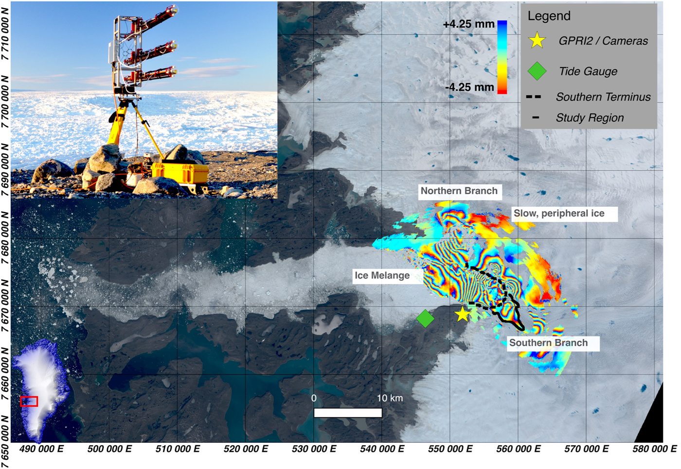
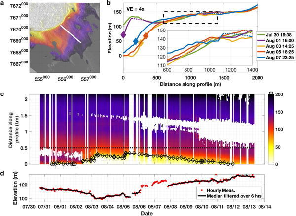
We performed an in situ study along the southern terminus of Jakobshavn Isbræ between 30 July and 13 August 2012. We deployed time-lapse cameras facing the glacier terminus and fjord, a tide gauge in the fjord, GPS receivers on the glacier surface and a terrestrial radar interferometer pointing at the glacier terminus (Fig. 1). Together, these sensors provide detailed observations of short-term variability in glacier terminus dynamics.
Differential interferogram superimposed on a Landsat 8 image of Jakobshavn Isbræ shows displacement during a 3 minute interval. The black polygon along the southern branch outlines the study region. (Inset) Photograph of the GPRI2 at the study site. Map projections are in Universal Transverse Mercator (UTM), zone 22 North.
Canon EOS DSLR cameras were used to document the timing of calving events. Four cameras photographed the terminus and ice mélange every 15 min during the field campaign and every 3 h throughout the rest of 2012. A fifth, high-rate camera was used to constrain the timing of calving events to within 10 s. A Global Water WL400 water-level sensor was deployed ~10 km downfjord of the calving front and sampled every 30 s.
A Gamma Remote Sensing Ground-based Portable Radar Interferometer II (GPRI-II) was used to measure the short-term changes in glacier speed and surface elevation. The GPRI-II is a Ku band (λ = 1.75 cm), real aperture, rotating radar interferometer capable of measuring surface deformation at a range of up to 16 km (Werner and others, Reference Werner, Strozzi, Wiesmann and Wegmuller2008). It has a range resolution of 0.75 m and an azimuthal resolution proportional to slant range at a ratio of 8:1000 (8 m at 1 km slant range). The GPRI-II has one transmit and two receive antennas (Fig. 1 inset). Interferograms produced between consecutive acquisitions using the same receive antenna are used to derive horizontal displacement, whereas interferograms generated between both receive antennas during a single acquisition are used to derive topography.
We used the TRI to image the terminus and proglacial fjord at 3 min intervals for 15 d; the timing of scans is controlled by a single-frequency GPS receiver integrated into the GPRI-II unit. We downsampled raw radar data by a factor of five in azimuth to account for oversampling, and then converted it to single-look-complex data (SLC). All SLCs were co-registered to the first image in the record, and then multi-looked, or averaged, by 15 pixels in range to reduce noise and generate square pixels along the southern terminus. The SLC data were then converted into line-of-sight (LOS) displacement and topographic interferograms, and later velocity maps and DEMs. All TRI images were reprojected from radar coordinates to 15 m Cartesian space in local Universal Transverse Mercator (UTM) projection and geolocated using corner radar reflectors surveyed with handheld Garmin GPS receivers. No correction was made for slant range because the small vertical look angle (5° below the horizontal) and low topographic relief in the viewing geometry have a negligible effect on ground range values (<0.5%). The methods used to generate the high-resolution time series are new and require several additional steps that are described in detail in Sections 2.1–2.2. Readers not interested in these finer details should skip to Section 2.3.
2.1. TRI-derived speeds
A total of 5579 interferograms were used to generate a 15 d record of speed. Most interferograms span 3 min, while a small percentage (~2%) span 5–6 min. Interferograms were smoothed with an adaptive filter (ADF) to minimize noise (Goldstein and Werner, Reference Goldstein and Werner1998). The filter preferentially favors pixels with high coherence, while penalizing less coherent pixels; we used a 32 × 32 pixel ADF window size, a 7 × 7 pixel correlation window size and an ADF exponent of one. We then used Goldstein and others (Reference Goldstein, Zebker and Werner1988) minimum cost flow method to unwrap the ADF-filtered interferograms, converting relative phase differences to true phase displacements. The complex deformational field along Jakobshavn Isbræ’s terminus (e.g. slow-moving ice sheet, fast glacier and ice mélange with variable speeds, frequent transients and distinct discontinuities) generates large gradients in phase that impede unwrapping algorithms. Consequently, many of the unwrapped interferograms contained erroneous branch cuts that led to discontinuities and 2π phase jumps. Such interferograms are typically excluded from interferometric studies; however, our objective was to maintain a high temporal resolution record of short-term variations. Therefore, additional steps were taken to eliminate these errors and consolidate 2π phase jumps to a single n2π range.
2.1.1. Eliminating branch cuts/unwrapping errors
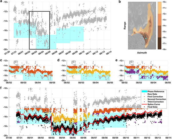
The raw phase values spanned many n2π cycles (Fig. 2a) for any given pixel and, in addition, were biased low. A lack of stable bedrock to provide a zero-reference point for the unwrapped phase led to phase values that were referenced to slowly deforming ice along the periphery, which underestimated the true unwrapped phase values. Therefore, we used a priori information to generate phase reference maps that contained the proper number of n2π integers for each pixel in the interferograms, the so-called Johnny Appleseed method (Hanssen, Reference Hanssen2001). The overlying assumption is that because fast flowing tidewater glaciers, like Jakobshavn Isbræ, are dominated by basal sliding and flow in a relatively smooth manner, frequent 2π step changes (the length of an interferogram fringe) over short 3 min intervals must be related to phase unwrapping and are not representative of glacier motion. Therefore, we exploit the dense number of observations and take a number of steps to correct for these short period errors in phase unwrapping while preserving the longer trend of phase changes.
Corrections to unwrapped phase. (a) Time series of raw unwrapped data (gray) at a discrete pixel show numerous unwrapping errors that manifest as 2π offsets; target phase reference ranges are indicated by cyan rectangles. (b) Sample target reference map with location of pixel used in this figure (cyan triangle). (c–e) Subsets of (a) showing the results after the first (orange), second (yellow) and third (purple) corrections. (f) The full time series, now with the spline curve (red) used to produce the final corrected unwrapped data (black). This example shows the correction for a single pixel, in practice the correction is applied to each pixel in the two-dimensional interferogram and for each time step.
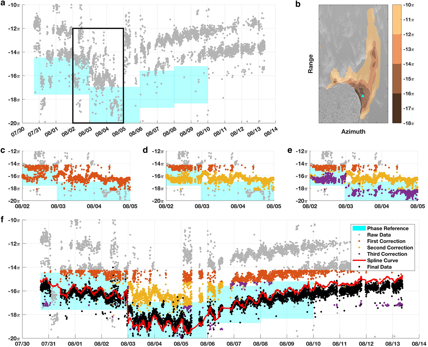
The radar's backscatter images, herein referred to as multi-look intensity images (MLI), are not affected by electromagnetic phase and thus can provide an independent measurement of surface displacement. We created phase reference maps (e.g. Fig. 2b) by speckle tracking MLI images in native polar geometry and then converting the speeds into LOS phase displacements over 3 min. We generated four reference maps to reflect the changes in the flow field that we observed in the raw unwrapped phase measurements (Fig. 2a): steady flow early in the record, step change and accelerated rates mid-record, and two maps to cover the gradual return to steady flow. The first, second and fourth maps were calculated using images 24 h before and after a nominal center time to minimize noise for each reference map. The third reference map was calculated by taking the mean of the second and fourth maps; this was necessary because of temporal gaps and a reduction in speed during this short time interval. The intervals and MLI images used for the reference maps are provided in Table 1. Samples of the n2π target phase range (cyan rectangles in Fig. 2a) from each reference map are shown for a discrete pixel; in practice, phase reference values were calculated for each pixel in the study area (Fig. 2b).
MLI acquisition times used for phase-correction target integer maps
The phase reference maps were used to systematically correct each unwrapped interferogram by collapsing multiple n2π phase values down to a single n2π range based on the reference map; these corrections were made sequentially. The first correction calculated the integer difference between the predicted and measured phase values, then adjusted the measured phase by n2π radians (orange in Fig. 2c). This effectively collapsed most of phase measurements to a single fringe (2π cycle) within the corresponding target range. Next, we corrected for ambiguity within a single fringe cycle and adjusted phase values that were more than half a fringe (>π radians) from the reference by 2π radians (yellow in Fig. 2d). This sometimes led to the rewrapping of phase measurements along the calving front, which re-introduced branch cuts and biased the phase measurements low by one integer cycle. To account for this, we assumed flow fields were continuous near the calving front and that differences were less than one fringe cycle and made a third correction (purple in Fig. 2e) to ensure the calving front had the same number of integer cycles as the ice a short distance behind it. Finally, we used a smoothing spline to fit a curve to the time series for the fourth correction (red in Fig. 2f); phase values more than 5.5 radians (0.9 integer cycles) from the curve were adjusted by 2π (black in Fig. 2f). The entire process generates interferograms with correct LOS phase displacements and few unwrapping errors; remaining residuals were later accounted for during stacking for atmospheric effects.
2.1.2. Atmospheric corrections
Variations in atmosphere between radar acquisitions can impact the index of refraction, which affects the two-way travel time of the electromagnetic wave and the measured phase. Typically, two atmospheric corrections are made: (1) a linear range correction that accounts for bulk atmospheric changes, and (2) a local correction to account for a heterogeneous atmosphere. We assume that bulk atmospheric variations are negligible over the short duration of our interferograms (minutes) and therefore neglect a range-dependent correction. We focus on the local variations within the radar's viewing geometry (heterogeneity in the atmosphere) and stack the phase measurements over a 21 min moving mean. We exclude pixels with phase values >1 Std dev. from the mean, and those with fewer than five measurements in the interval.
2.1.3. LOS to along-flow motion in UTM coordinates
Polar (azimuth, range), atmospherically corrected interferograms were reprojected to Cartesian coordinates and rotated into local UTM coordinates. As mentioned, corner reflectors were surveyed with handheld GPS receivers and used to coregister the images. Next, we used a python-based speckle-tracking tool, PyCORR (Fahnestock and others, Reference Fahnestock2016), to define the horizontal components of motion, which were used to convert LOS phase displacements to speed in the direction of flow. The component vectors were used to calculate ξ, the direction of flow and then θ, the difference between the flow direction and the LOS look angle. Two pairs of MLI GeoTIFFs were used to generate a complete map of θ values. The majority of the map was comprised using data from an 8 August 13:45 to 9 August 13:45 image pair, a time when the calving front was in an advanced position and velocity variations were minimal. Katabatic winds on 6 August rotated the TRI on its tripod, which resulted in the loss of measurements along the southern edge of the fast-flowing region; therefore, component vectors from a 30 July 16:22 to 31 July 16:21 image pair were used to supplement θ values during this time period. To minimize artifacts due to subtle flow differences between the two time periods, the hybrid θ map was passed through a 20 × 20 pixel Gaussian low-pass filter using a Std dev. of 2. LOS speeds were then divided by cos(θ) to calculate speed in the direction of flow in units of m d−1.
2.1.4. Error in TRI-derived speeds
Error sources for the TRI-derived speeds include phase unwrapping, LOS to along-flow conversion and atmospheric effects. Phase unwrapping errors were minimized using speckle-tracked polar reference images (see Section 2.1.1); this reduced errors to within the one integer cycle or ~4.1 m d−1. We assumed flow vectors remained constant over the study period and used a single θ map to convert LOS speeds to along-flow. PyCorr-derived velocity fields calculated for 11 of the 15 d reported Std dev. in flow direction of 5–8° over time, which translates to errors in the speed of 9.0–15.6%. Steps were taken to minimize atmospheric phase noise (see Section 2.1.2); however, estimates of atmospheric phase contribution are difficult to quantify due to a lack of stable reflectors (e.g. exposed bedrock) along the southern terminus.
The values above provide conservative error estimates from individual sources. To provide a more comprehensive estimate, we evaluated the total error by comparing phase-derived speeds with: (1) on-ice GPS measurements and (2) speckle-tracked speeds. GPS data were available for the last 3 d of observation and provide an independent measurement of speed. Three receivers were located 2.5, 2.1 and 3.6 km behind the 9 August calving face. RMSE between each GPS sensor and the corresponding pixels in the phase-derived speeds was 2.5, 2.3 and 2.3 m d−1, and mean absolute errors (MAE) were 2.3, 2.1 and 2.0 m d−1, respectively. To evaluate the early record, we compared the phase-derived speeds with speckle-tracked velocities derived from TRI intensity images, which are not susceptible to atmospheric phase noise and do not require a LOS conversion. Comparisons were made between PyCORR-derived speeds and mean speeds from phase-derived measurements calculated for four different 24 h intervals with center dates: 31 July 4:22, 1 August 5:22, 2 August 00:22, 9 August 00:21. For each interval, differences in speed had a normal distribution with RMSE and MAE (in parentheses) values of 3.6 (3.5), 3.8 (3.2), 3.2 (3.0) and 3.5 (3.0) m d−1, respectively. Based on GPS and speckle-tracked comparisons, we adopt a conservative estimate in a total error of 3.8 m d−1, which is a little less than a full integer offset (4.1 m d−1).
2.2. TRI-derived surface elevation changes
The GPRI-II has two receive antennas vertically spaced by 25 cm (bottom antennas in Fig. 1 inset). Concurrent measurements from both antennas can be used to generate DEMs without the need for atmospheric and phase displacement corrections. We used the dense record of topographic interferograms to generate multiple DEMs following the methods of Strozzi and others (Reference Strozzi, Werner, Wiesmann and Wegmuller2012). We then differenced all DEMs from the first DEM to track changes in surface elevation over time. To minimize noise, we ADF filtered the interferograms, stacked for each hour of observations and excluded pixels with coherence <0.9.
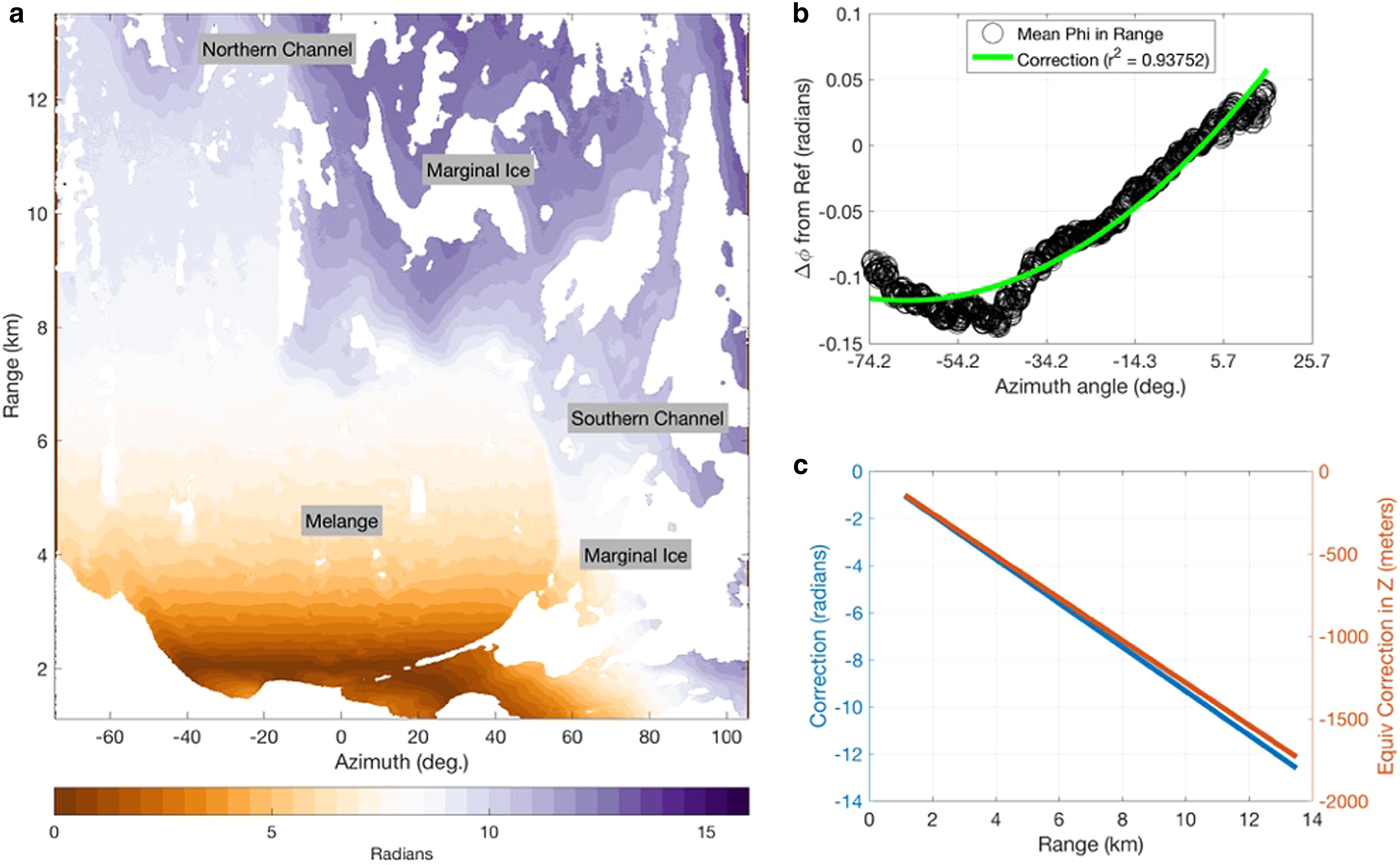
High-quality DEMs require perfect vertical alignment of the TRI instrument. Despite our best attempts to secure the instrument and maintain perfect vertical alignment, the combined effects of wind stress, thermal variability and the instability of the till surface upon which the TRI was mounted led to deviations in vertical alignment over time. As a result, biases in azimuth (Fig. 3b) and range (Fig. 3c) were observed in the maps of mean phase. Two corrections were made to remove the bias in the topographic stacks: a quadratic correction in azimuth to account for the variation in the tilt over 15 d, and a linear correction in range to account for the initial error in vertical alignment. For the non-linear correction, we difference each intefergram stack from the first hour and then calculate the median phase in range along each azimuth step (Fig. 3b, black circles); we exclude near and far-field range values and those >1 Std dev. to minimize noise. We then fit a quadratic curve (Fig. 3b, green curve) to the residuals and use it to correct for the variations in tilt.
Topographic phase correction for DEM alignment errors. (a) One-hour stack of topographic interferograms in polar coordinates before correcting for tilt (range) and bowtie (azimuth) effects. Sample corrections in (b) azimuth and (c) range applied to each mean phase map.
To correct for the initial error in vertical alignment, we used a ground control point located at the same elevation as the TRI. Pixels with stable bedrock make ideal ground control points; however, the bedrock points in the radar viewing geometry were all lower than the TRI. Therefore, we identified a pixel in the slow, peripheral ice that appeared in both Google Earth images and the topographic stack. The phase was sampled at the ground control point and added back into the mean phase values to generate the DEMs. The DEMs were adjusted by the GPRI-II elevation and filtered. We used a Gaussian filter to remove high-frequency noise and interpolated for pixels with no data to generate a smooth and continuous DEM. Lastly, the DEMs were converted to GeoTIFFs in local UTM coordinates; all elevations are in height above sea level. Elevations sampled at six locations on stable bedrock near the north channel report Std devs. from 2.5 to 2.9 m. However, these points are >12 km in range, and thus are expected to be significantly higher than values along the southern channel (4–7 km in range) due to the linear decrease in spatial resolution with range. A better evaluation of error is the variability within slow-moving ice in the near field (2 km range) and in the peripheral ice adjacent to the southern channel (~8 km in range), where changes in surface elevation are primarily due to surface melt and are expected to be minimal over our short observation period. Std devs. ranged from 0.47 m in the near field to 0.99 m along the peripheral ice; we conservatively adopt the latter as the nominal domain-wide error.
2.3. Mapping calving events and terminus location from TRI
The radar's MLI images were used to map terminus locations. The calving front was manually digitized in MATLAB using the techniques of Cassotto and others (Reference Cassotto, Fahnestock, Amundson, Truffer and Joughin2015). The terminus was sampled every 6 h with increased sampling around calving events. Calving losses were calculated by comparing front positions immediately before and after calving events, summing the number of pixels lost to calving, and then multiplying by the area of each pixel (225 m2). The result is a record of calving losses that is well constrained in time and 2-D space but does not fully capture submarine calving events. The record of terminus positions was supplemented with Landsat panchromatic images (band 8) to extend the record in time, albeit with decreased temporal resolution.
3. RESULTS
3.1. Calving record
A total of 13 calving events occurred during the study that ranged in size from 0.01 to 1.43 km2 (Table 2); 11 events were observed with the high-rate camera, two events (31 July 10:30 and 1 August 22:13) were not. The majority of calving events were slab capsizes with a predominantly backwards rotation (basal ice rotates in the downfjord direction while the surface rotates in the up-glacier direction). Furthermore, several calving events included a combination of serac failures, submarine events and forward rotating slabs; each lasted for several minutes and were cascading in nature (Movie S1 in supplemental materials).
Characterization of calving events
3.2. Short-term variations in speed
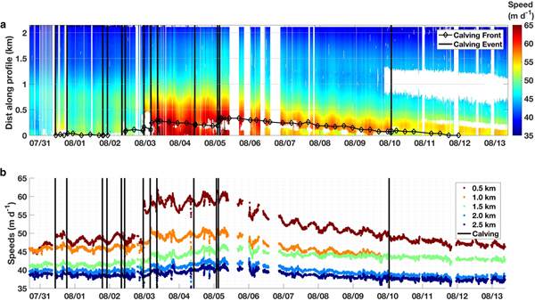
Speeds along a central flowline varied from 65 m d−1 at the terminus to 35 m d−1 2 km up-glacier (Fig. 4a). Of the 13 calving events observed (black vertical lines in Fig. 4), most produced no obvious change in speed. However, the calving event at 23:10 on 2 August resulted in a very small (~40 m) retreat of the calving front and led to an immediate step change in flow. Speeds increased by as much as 30%, remained high for several days, and then gradually slowed to pre-calving speeds. A time series sampled at 0.5 km steps along the same profile shows the response was not uniform throughout the terminus (Fig. 4b). Rather, the change in speed was largest at the calving front, decreasing to no resolvable change 2 km up-glacier.
Time series of speed. (a) Center flowline speeds along Jakobshavn Isbræ’s terminus; the location of the calving front (black diamonds) and timing of calving events (black lines) are shown. (b) Speed at 0.5 km steps along the profile. Location of the flowline is shown in Figure 6.

A semi-diurnal signal was observed in the data, indicating that ice flow was tidally modulated. The 2 August 23:10 calving event enhanced this signal; speeds 0.5 km along the profile varied 2 m d−1 peak-to-peak prior to calving (dark red in Fig. 4b), but then increased to 4 m d−1 peak-to-peak immediately after calving.
3.3. Response to calving
To further investigate glacier response to calving, we sampled speeds 3 h before and after calving at a pixel nominally 0.5 km from the terminus (~0.4 km from the terminus on 3 August). We found that the glacier experienced a step increase in speed immediately after five calving events (Fig. 5c). Three of these calving-induced speed-up events: 31 July 10:30 (1.43 km2), 3 August 03:58 (0.56 km2) and 5 August 1:44 (1.31 km2), were among the largest in our record, and all increased speeds by ~10%. In contrast, the remaining two events were small but produced the largest increases in speed: the 2 August 23:10 (0.08 km2) event was one-sixteenth the size of the largest event and resulted in a 30% increase in speed; the 3 August 8:36 (0.01 km2) was the smallest event but resulted in a 12% increase in speed. The remaining calving events were relatively small and produced no resolvable changes in speed.
Characterization of calving events. (a) Polygons highlighting calving area losses for select events; (b) the relative size and spatial distribution of all calving events mapped by the centroid; (c) change in speed during calving events; legend indicates the time and areal size of events; (d) instantaneous change in speed vs calving area loss.
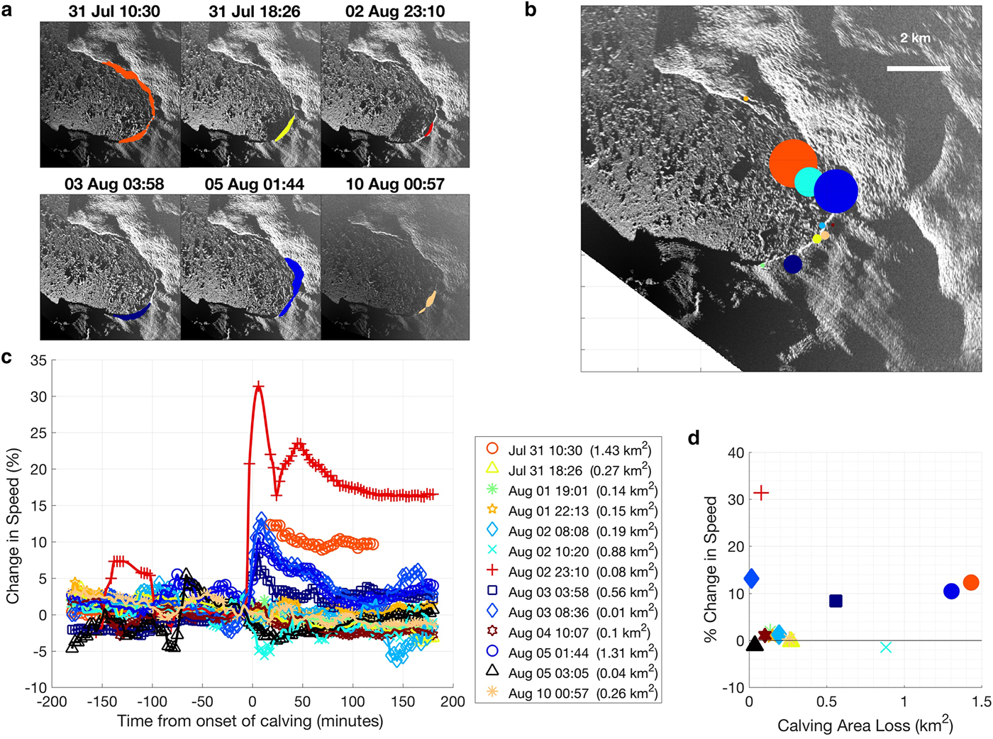
We found no correlation between calving area loss and the change in glacier speed (Fig. 5d). However, all five of the speed-up events occurred after calving from a highly localized region (~20% width of the calving face) near the center of the terminus (Figs 5a, b), and all involved the calving of dirty and/or basal ice (Movie S2). Three of these events: the 2 August 23:10 (main event), 3 August 3 03:58 and 3 August 8:36, occurred within a 10 h span, and two were exceptionally small and resulted in little change in terminus position and shape. The other two calving-induced speed-up events, 31 July 10:30 and 5 August 1:44, calved significantly more ice along the periphery, but also from the same center region as the three smaller events (Fig. 5a).
3.4. Dynamic changes in surface elevation
Repeated centerline profiles show large variations in surface elevation (Fig. 6b). Initially, the ice immediately behind the calving face (out of view) was 105 m tall (30 July, green). Following a 100 m retreat, elevations at the calving face decreased to 71 m (1 August, purple). By 3 August (yellow), the calving face retreated an additional 260 m and reduced to 45 m in elevation. The glacier retreated to a minimum position on 5 August (red), but the calving face was now 67 m high. By 7 August (blue), the terminus re-advanced, and the height of the calving face reduced to 48 m.
Variations in surface elevation. (a) Map of surface elevations with the location of a profile (white line) sampled in (b–d). (b) Cross-sections of surface elevations along the profile for five different epochs, dashed lines show interpolated values for missing data; note the reverse surface slope prior to calving in the early record. (c) A time series of surface elevations along the profile. (d) Time series of elevations 0.5 km along the profile. Diamonds in (b) and (c) indicate the location of the calving front.
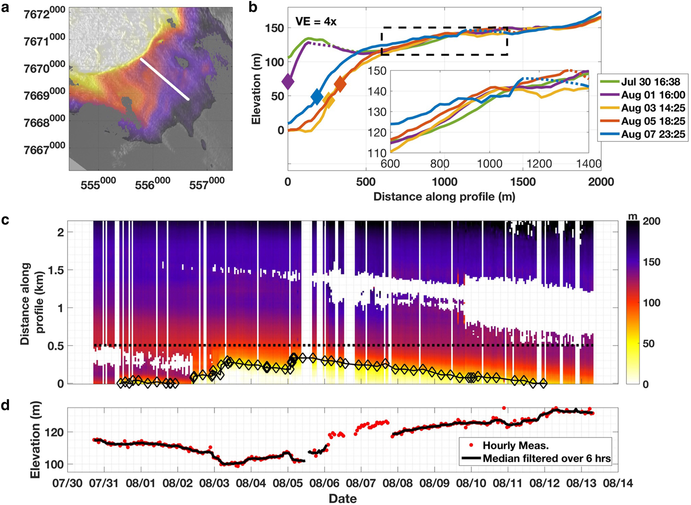
Farther up-glacier, the pattern of elevation change was much different; surface elevations between 600 and 900 m along the profile (inset in Fig. 6b) steadily increased with time. A reverse surface slope, sometimes indicative of impending calving events (Rosenau and others, Reference Rosenau, Schwalbe, Maas, Baessler and Dietrich2013; James and others, Reference James, Murray, Selmes, Scharrer and O'Leary2014; Xie and others, Reference Xie2016), was observed along the terminus in the early profiles and was absent in later measurements.
A plot of surface height along the centerline through time (Fig. 6c) shows a progressive increase at the terminus following the 2 August 23:10 calving event and initial speedup. This pattern emerged in the middle of the record and continued through the end. It coincided with a re-advance of the terminus and implies the advection of thicker ice toward the calving front. A time series sampled 0.5 km up-glacier shows that surface elevation was generally stable during the first few days (Fig. 6d), started to decrease on 2 August, and then abruptly decreased ~10 m on 3 August, coincident with the three calving-induced step changes in speed on 2 August and 3 August. Surface elevations then increased for 2 d before a second abrupt decrease in surface elevation on 5 August. Noise precludes assessment on 6–7 August, but surface elevations had increased 18 m by 8 August (>10 m above 2 August elevations) and continued to increase.
4. DISCUSSION
Determining why some calving events triggered step changes in speed and dynamic thinning while others did not is critical to our understanding of glacier dynamics. To address this question, we investigate the conditions leading up to the largest calving-induced step change in speed (2 August 23:10 event) and the spatiotemporal variations in speed, strain rate, surface elevation and tidal response along the terminus. Finally, we compare our results with satellite-based observations to provide context for our study.
4.1. A trigger to fast flow
Few of the 13 calving events were of the large, full glacier width, full glacier thickness calving style previously described at Jakobshavn Isbræ (e.g. Amundson and others, Reference Amundson2008, Reference Amundson2010). Instead, most were confined to localized regions that removed small portions of the terminus (Fig. 5a). Furthermore, the timing and spatial coincidence of smaller events that led to step changes in speed suggests that bed topography was an important control on the dynamic response to calving.
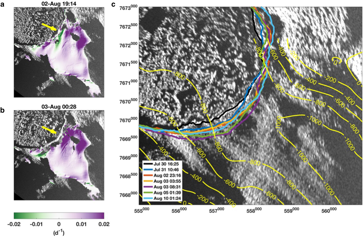
Jakobshavn Isbræ generally calves ice from a grounded terminus in late summer (Amundson and others, Reference Amundson2008). Photographic evidence of sediment strata in the basal layers of freshly calved icebergs (Movie S2) indicate the majority of the terminus was grounded; this is because icebergs calved from floating termini are generally devoid of sediments due to submarine melt processes. Thus, a small-scale retreat of the terminus behind a bedrock obstruction may have reduced basal and lateral resistance and led to an increase in speed. TRI-derived surface strain rates show a compressional band (Fig. 7a, green) within a predominately extensional zone (Figs 7a, b – purple). This band briefly switched to extensional following the 31 July 10:30 calving event, the largest observed, but then returned to compressional for several days thereafter (Movie S3). Compression increased after the 2 August 8:08 calving, then reversed to an extensional regime following the 2 August 23:10 calving event (Fig. 7b; Movie S3). It remained extensional for several days before it gradually transitioned back to compressional by the end of the record. This area coincides with a tapered section of the bed (Fig. 7c; Morlighem and others, Reference Morlighem2017); the series of calving events that began on 2 August led to a small retreat of the terminus from a narrow constriction in the bed into a wider, less restrictive channel, which impacted the pattern of surface strain rates, and by inference basal and lateral drag along the bed. This suggests that the geometry of Morlighem and others bed model is accurate in this section of the fjord. It further indicates that bed geometry strongly impacts Jakobshavn Isbræ’s response to calving, as has been shown for other tidewater glaciers (Enderlin and others, Reference Enderlin, Howat and Vieli2013, Reference Enderlin, O'Neel, Bartholomaus and Joughin2018).
Bed topographic trigger to fast flow: step changes in speed occurred as the terminus retreated into subtly wider region of the bed. Longitudinal strain rates (a) before and (b) after the 2 August 23:10 calving event; purple indicates extension, green compression, yellow arrows show the location of calving event. (c) Front positions (colored lines) and Morlighem and others, (Reference Morlighem2017) bed model (yellow contours) overlain on an MLI image.
4.2. Spatiotemporal variations in speed, strain rate and elevation
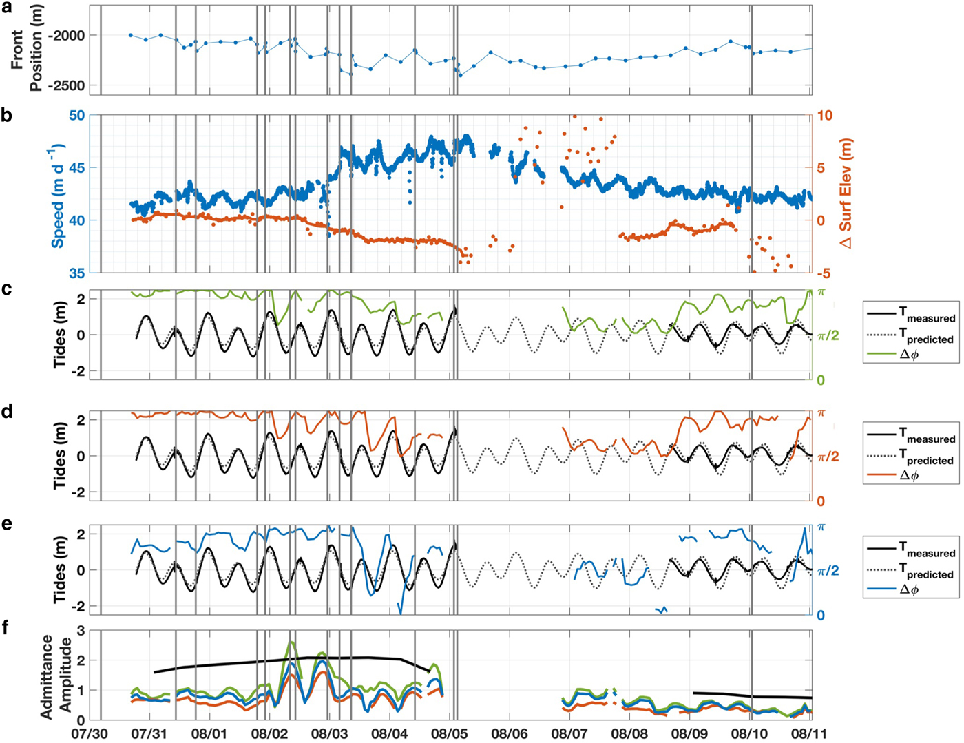
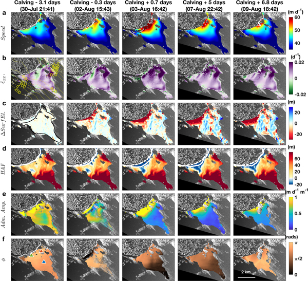
In a density-conserving fluid, such as a glacier, changes in strain rates must lead to changes in thickness, which have implications for terminus stability. We now look at spatiotemporal variability in speed, strain rates, surface elevation (ice thickness) and the height above flotation (HAF; Fig. 8); Section 4.3 compares these patterns against maps of tidal forcing (Figs 8e, f).
Spatiotemporal variations around 2 August 23:10 calving event. (a) Speeds, (b) longitudinal strain rates (purple = extension, green = compression), (c) surface elevation changes, (d) height above flotation (HAF) with the corresponding (white lines) and 30 July 16:22 (white dashed line) front positions shown for reference, (e) tidal admittance amplitude, and (f) tidal admittance phase lag. Contours in (b) represent bed elevations from Morlighem and others, (Reference Morlighem2017); polygon in (c) indicates 9 km2 sample area shown in time series in Figure 9b; colored triangles in (f) show the location of tidal admittance sampled in time series in Figure 9.

Variations in stability through feedbacks along the terminus. Time series of (a) mean front position relative to 2012 maximum, (b) speed and surface elevation changes measured from beginning of the record over a 9 km2 patch of the ice stream (Fig. 8), (c–e) the phase lag between tides and ice speeds, and (f) admittance amplitude for three locations along the terminus (Fig. 8f); black lines in (f) indicate the tidal amplitude (see text). Gray vertical lines throughout indicate the timing of calving events.
Speeds showed spatiotemporal variability throughout the record. Overall, speeds were fastest near the calving front (Fig. 8, row a) and within the deep, narrow channel in Morlighem and others (Reference Morlighem2017) bed model (yellow contours in Fig. 8b). Temporally, speeds were moderate during the early record, peaked after the 2 August 23:10 calving, then gradually decreased with the region of fast flow becoming more localized through the end of the record. Early on, a slower moving patch of ice appeared where the bed widens upstream, down-glacier of the compressive patch and near the glacier center. It disappeared following the 2 August 23:10 calving event, but a second patch emerged farther up-glacier and advected toward the calving front (Movie S3).
Variations in longitudinal surface strain rates accentuate the spatial variations in speed (Fig. 8, row b). The majority of the terminus was under extension while compressional bands appeared ephemerally near the calving front (see Section 4.1). The highest extensional rates occurred within the narrow channel and intensified after the 2 August 23:10 calving event. Weak bands of extensional strain also appeared near the glacier center; the magnitudes varied but decreased as the terminus re-advanced into the narrow constriction. Thus, small changes in terminus position led to significant fluctuations in strain rate.
The largest decrease in surface elevation that occurred at the mélange–glacier boundary represents calving retreat (Fig. 8c). The remaining elevation changes reflect the impact of spatiotemporal pattern in strain rates and advection. Surface lowering was observed behind the calving front, within a patch behind the fast-flowing region, and along a thin band that extended south from this patch. In contrast, adjacent areas show an increase in elevation (blue), which created a hummocky surface topography with the same oblique orientation to flow as the strain rate patterns (Movie S3). The majority of ice thickened by the end of the record, indicating a strong advective effect. The magnitude of these changes (about ±15 m over 7 d) is consistent with previous studies (Joughin and others, Reference Joughin2012), albeit over much shorter timescales (e.g. weekly vs annual). This suggests that short-term variations in ice dynamics are a significant contribution to the annual drawdown. The observations of localized dynamic thinning further demonstrate Jakobshavn Isbræ’s high sensitivity to small variations in bed topography.
Spatiotemporal variations in ice thickness impact the HAF, a metric often used to assess basal coupling and glacier calving (e.g. van der Veen, Reference van der Veen1996). A glacier that is well above flotation has significant overburden pressure that exceeds subglacial water pressure. As a tidewater glacier thins and overburden pressure decreases, the terminus approaches buoyancy, which reduces basal traction. Early in the record, large extensional strain rates thinned the glacier and decreased the HAF in a key area behind the southwest caving front (Figs 8b, d; Movie S3). The 3 August 03:58 calving event removed considerable ice along the southwestern calving front and moved the calving face to a patch of ice already below flotation (blue in Fig. 5a). As a result, basal coupling was reduced along much of the calving face, which helped sustain high speeds for several days. Eventually, thicker ice advected into this region and the adjacent area (Fig. 8c) where already thick ice occupies the large overdeepening in the bed (Fig. 8b). This increased the HAF (Fig. 8d; Movie S3), enhanced basal coupling and led to slower speeds (Fig. 8a). Thus, a localized patch near the calving front had the greatest impact on basal coupling, which highlights the importance of spatial variations in the HAF and the sensitivity of this system to small changes in ice thickness, both of which reiterate the significance of small changes in bed topography.
4.3. Changes in tidal-induced flow
The time series of speed (Fig. 4) shows an increase in semi-diurnal variation following the 2 August 23:10 calving event. Changes in basal coupling, as discussed above, should manifest in the glacier's response to ocean tides. We calculated the tidal admittance to characterize the impact of tidal forcing. Tidal admittance is a harmonic analysis between the ice speed and an individual constituent of ocean tides (Walters and Dunlap, Reference Walters and Dunlap1987; O'Neel and others, Reference O'Neel, Echelmeyer and Motyka2001; de Juan and others, Reference de Juan2010; Podrasky and others, Reference Podrasky, Truffer, Luthi and Fahnestock2014). It is expressed as a ratio of the amplitudes of ice speed and the tide in units of m d−1 m−1, and the difference in phase (tides minus glacier speed) in radians. Admittance amplitude quantifies the magnitude of tidal forcing, while variations in the admittance phase reflect changes in basal drag (O'Neel and others, Reference O'Neel, Echelmeyer and Motyka2001). A phase lag of zero, indicating glacier speeds that correlate with the tides (high tide = fast flow), reflects a water pressure impact on sliding, and thus weak coupling to the bed. A phase lag of π, anticorrelation (low tide = fast flow), suggests strong basal coupling or a higher sensitivity to the increase in backpressure on the calving face than the change in basal water pressure. We used t_tide (Pawlowicz and others, Reference Pawlowicz, Beardsley and Lentz2002), a MATLAB-based harmonic analysis tool, to perform the calculations on the M2 principal lunar semi-diurnal tide, the dominant tidal constituent in the fjord. We re-created the tidal record using t_predict, a tidal prediction tool packaged with t_tide. This was necessary to avoid transient noise in our water-level measurements related to glaciogenic ocean waves, and to account for a power failure between 5 and 8 August. We sampled 24 h running windows of TRI speeds and passed them through t_tide to calculate the admittance amplitude and tidal phase differences. Pixels having a signal-to-noise ratio of <0.5 were removed to reduce noise. In addition, we discarded values from 5 to 6 August due to data gaps that preclude adequate sampling for the harmonic analysis. Maps of the admittance amplitude and phase lag are shown in Figures 8e, f.
In general, admittance amplitudes were highest near the calving front (>1 m d−1 m−1; Fig. 8e) and decreased up-glacier (~0.5 m d−1 m−1), and phase was anticorrelated with the tides (Fig. 8f). This suggests that the terminus was grounded and that semi-diurnal changes in water depth modulated terminus speeds by varying the height of the resisting water column along the calving face (Hughes, Reference Hughes1989). We observed variations in admittance amplitude and tidal phase over time, indicating changes in terminus stability over time. For example, brief periods of higher admittance amplitudes and reduced phase lag were observed leading up to the 2 August 10:20 and 23:10 calving events (Movie S3). We infer the decrease in basal drag indicates an approach to flotation in the hours preceding the calving events, as has been hypothesized as a prerequisite for calving in previous studies (van der Veen, Reference van der Veen1996; Vieli and others, Reference Vieli, Jania and Kolondra2002; Nick and others, Reference Nick, van der Veen and Oerlemans2007; Xie and others, Reference Xie2016). Over the next several days, the admittance amplitude and the phase lag were reduced; the latter suggesting the terminus moved closer to flotation.
4.4. Dynamic processes, feedbacks and short-period instability
There are two ways to impact the flotation thickness of a glacier: (1) via melt and dynamic stretching of the terminus, and (2) by increasing the subglacial water pressure sufficiently to reduce the effective pressure, thereby reducing basal drag. In this section, we explore these possibilities through multiple time series.
The mean front position shows little variation during the first few days despite several calving events (Fig. 9a). Mean speeds (panel b, blue) and the change in elevation (orange) averaged within a 9 km2 polygon (Fig. 8b) show small fluctuations but were generally stable. The surface lowered 1 m on 2 August, another meter on 3 August, then stabilized for a couple of days before it lowered an additional 1.3 m on 5 August. Speeds reached peak levels between 2 and 5 August, coincident with a ~400 m calving retreat. The terminus then started to re-advance and speeds began to slow. Noise in the DEM record precludes accurate surface elevation measurements on 6–7 August, but elevations were notably higher on 8 August and continued to increase as the calving front re-advanced and speeds gradually decreased. By 9 August, the terminus had re-advanced to its 2 August location and the elevation within the polygon was within 0.4 m of pre-calving elevations.
Variations in the tidal admittance sampled at three locations (Fig. 9) demonstrate a change in the basal coupling, likely due to the changes in ice thickness, beginning on 2 August. Phase lag at all three locations (Figs 9c–e) remained close to π for the first several days, indicating the terminus was well coupled to the bed. However, a dip in phase and subsequent increase in admittance amplitude indicate the terminus moved closer to flotation leading up to the 2 August 10:20 and 23:10 calving events (decreased coupling), and then moved away from flotation (enhanced coupling) after the calving events (Fig. 9f). Coincident with the onset of rapid thinning on 3 August, the phase reduced and stayed low for several days (decreased coupling) indicating the terminus was close to flotation. By 9 August, as the calving front re-advanced to its 2 August position, the mean change in surface elevation (thickness) returned to 2 August levels, and the phase lag moved closer to π.
The change in tidal admittance represents a shift in the tidal forcing mechanism. Semi-diurnal variations in water depth still affect the balance of forces along the calving face; however, subglacial water pressure plays a more significant role after the dynamic changes in ice thickness on August 2 and 3. High tides increased the subglacial water pressure and lowered basal friction that favored flow, while low tides led to lower subglacial water pressures that increased basal friction and retarded flow. Thus, sliding became increasingly sensitive to changes in effective pressure as the glacier approached flotation. These variations in tidal admittance demonstrate an evolution in terminus stability that is directly related to feedbacks between ice thickness and speed variations over 15 d.
Large changes in ice thickness that occur over short time periods (e.g. daily) can only be explained by ice dynamics. The rapid thinning on 3 August occurred because of an abrupt shift in strain rates from an alternating pattern of compressional and extensional regimes to purely extensional flow (Figs 7a, b), which led to dynamic thinning (Fig. 9b) and sustained high flow rates. Several days later, surface elevations (ice thickness) began to increase as the calving front re-advanced. This implies that an advective component to the thickness change, which helped reduce speeds and re-stabilize the terminus. A large overdeepening in the bed up-glacier of the calving front (e.g. Fig. 7c), coupled with the lack of a surface depression, suggests that thick ice was located a short distance up-glacier of the calving front and could easily be advected toward the front to help stabilize the terminus after rapid dynamic thinning events.
Finally, the majority of observed calving events occurred during a spring tide, which is indicated by the high tidal amplitudes (black line in Fig. 9f) between 30 July and 5 August. This suggests a tidal influence on calving; however, these observations could also reflect a more complex relationship between the tides, the proglacial ice mélange and calving.
4.5. Transient perturbations and long-term change
Podrasky and others (Reference Podrasky2012) showed that short-term perturbations in flow can impact Jakobshavn Isbræ’s behavior over much longer time scales. We compared our results with satellite and time-lapse camera observations to examine how the calving-induced step change in speed that we observed relates to a longer record of glacier velocities.
Jakobshavn Isbræ retreated ~18 km between 2002 and 2012 (Figs 10a, b), and then another ~1 km by 2013. Since then, the calving front has seasonally varied ~3 km, but maintained the same approximate position in the fjord. Satellite-derived terminus positions (Fig. 10c, orange) show a progressive retreat in 2012 that peaked in July; this was the most retreated position since before the Little Ice Age (1500–1900 A.D.) (Sohn and others, Reference Sohn, Jezek and van der Veen1998; Weidick and others, Reference Weidick, Mikkelsen, Mayer and Podlech2004) and perhaps the mid-Holocene (Weidick and Bennike, Reference Weidick and Bennike2007; Briner and others, Reference Briner, Stewart, Young, Philipps and Losee2010; Young and others, Reference Young2011). Time-lapse cameras show a calving hiatus between 11 July and 27 July, during which the terminus advanced 400 m. Single calving events occurred on 28 July and 30 July before a series of calving events in early August, coincident with our TRI observations. The 2 August 23:10 calving event put the calving face 100 m downfjord of the 11 July minimum (Fig. 10c), and several additional events over the next 3 d forced a retreat to the 11 July position. Calving ceased on 5 August, and the terminus re-advanced.
Long-term implications of short-term perturbations. (a) Seventeen-year history of terminus positions with a time series of mean front positions in (b); (c) 2012 mean front positions from satellite and GPRI; (d) time series of satellite-derived speeds from NASA MEaSUREs.
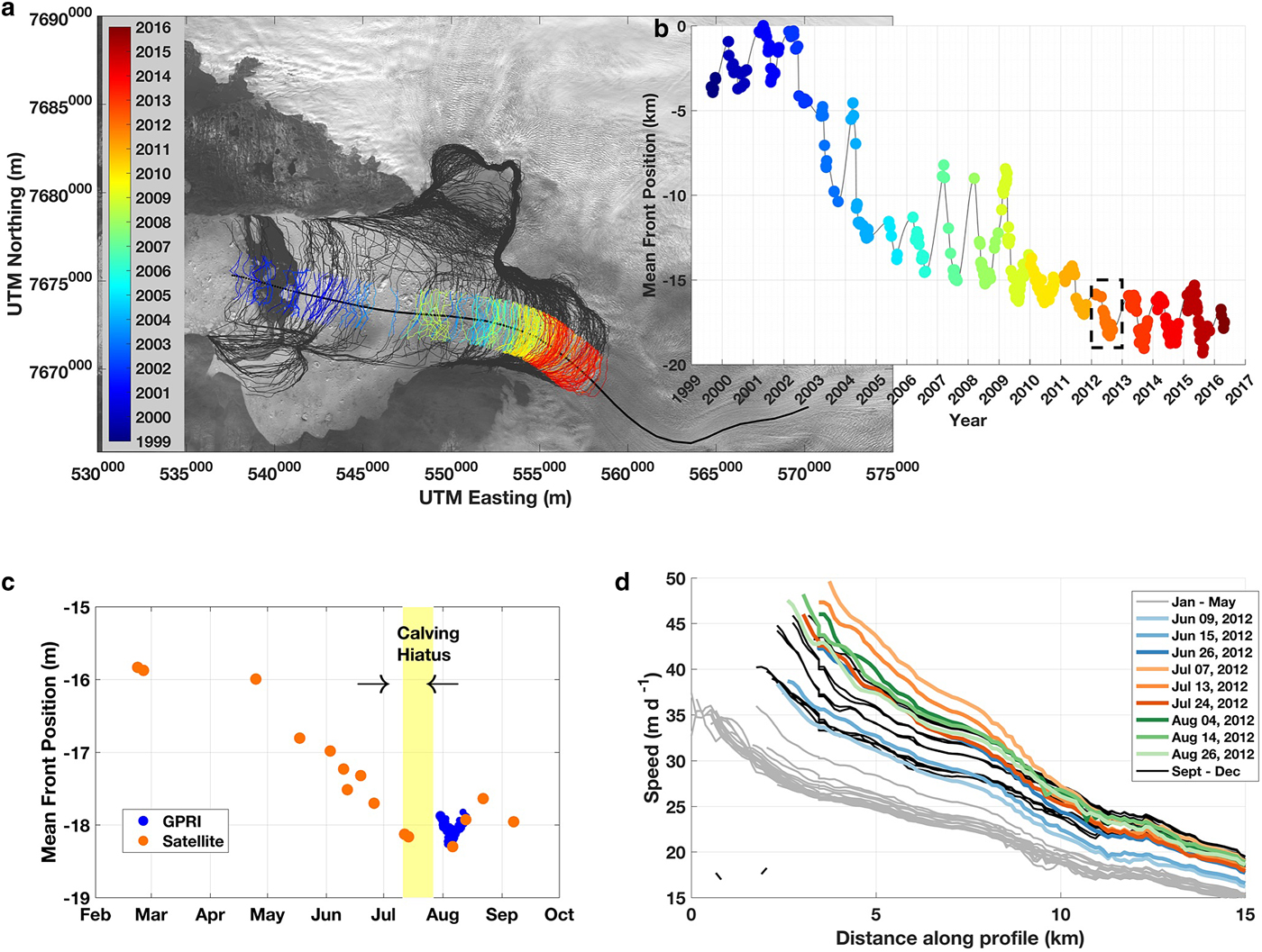
TerraSAR-X (TSX) speed profiles from the NASA MEaSUREs dataset (Joughin and others, Reference Joughin, Smith, Shean and Floricioiu2014) were sampled along a center flowline and plotted by center date (Fig. 10d). Speeds were at a minimum between January and May (gray) and ranged from 35 m d−1 at the calving face to 10 m d−1 20 km up-glacier. Speeds increased through June (blue profiles) and peaked at 50 m d−1 by 7 July (light orange). Speeds were slightly lower on 12 July (orange), followed by a significant reduction by 24 July (dark orange). By 4 August (dark green), speeds increased to a second peak that summer, then slowed in late August (light greens) and remained low for the remainder of the year (black).
These satellite and camera records show that Jakobshavn Isbræ experienced two peaks in speed that summer, which coincide with a retreat of the calving front behind the same bed constriction in the fjord (e.g. Fig. 10c). The records show a small re-advance occurred between the two peaks that positioned the terminus in the narrow bed constriction. Serendipitously, our TRI measurement period coincides with TSX acquisitions on 30 July and 10 August; our measurements of a small calving event that triggered a step increase in speed captured the second peak in speed that summer. As the calving front re-advanced into a narrow section of the bed on 9 August, speeds slowed with the terminus further from flotation and basal coupling enhanced. Based on these observations, we infer that a similar and perhaps larger dynamic response may have occurred during the July peak in speed, producing the highest speeds ever recorded at this glacier (Joughin and others, Reference Joughin, Smith, Shean and Floricioiu2014). Extrapolating our results further, similar processes may explain the recent lack of continued terminus retreat and speedup (Joughin and others, Reference Joughin, Smith and Howat2018). Beginning in 2012, calving started to occur further into the deep channel where very thick ice (>1 km) occupies an overdeepened section of the fjord (e.g. Fig. 10c). If the seasonal speedup of Jakobshavn Isbræ also enhances advection, as suggested here, then ice dynamics may be stabilizing the terminus by delivering enough ice to sufficiently increase the HAF following perturbations in speed. By compensating for the strain-induced increases, advection of thicker ice may stabilize the terminus, thereby reducing speeds and preventing further retreat.
5. IMPLICATIONS FOR TIDEWATER GLACIER STABILITY
Our study has several implications. First, a small calving retreat of a tidewater glacier terminus can generate large variations in speed and therefore ice thickness and stability. While episodic events such as large calving events (Scambos and others, Reference Scambos, Bohlander, Shuman and Skvarca2004; Amundson and others, Reference Amundson2008; Nettles and others, Reference Nettles2008; de Juan and others, Reference de Juan2010) or the loss of a floating tongue (Joughin and others, Reference Joughin, Abdalati and Fahnestock2004) are known to trigger dynamic changes along the terminus, we show that a smaller calving event that removed significant basal ice initiated a return to historically high flow rates. This represents a consequence of the continued drawdown along Jakobshavn Isbræ and therefore may be specific to glaciers that are close to flotation. However, many of Greenland's tidewater glaciers have been thinning since the early 2000s (Pritchard and others, Reference Pritchard, Arthern, Vaughan and Edwards2009), and may be susceptible to similar large-scale response to small perturbations.
A second implication is that bed topography plays an important role in the response of a tidewater glacier to perturbations along the terminus. The influence of bed geometry on fast tidewater glacier flow has long been recognized (Meier and others, Reference Meier, Post, Rasmussen, Sikonia and Mayo1979); the funneling of ice from vast, unconfined regions of the interior through long, narrow, bedrock channels generates large driving stresses in outlet glaciers. Our study demonstrates that even subtle changes in terminus position (e.g. a few hundred meters) can have a profound effect on speed.
Third, advection processes can stabilize a tidewater glacier by counteracting dynamic thinning losses due to enhanced strain rates. Increases in strain rate enhance dynamic thinning, which promotes faster flow, additional thinning and greater instability via a positive feedback. However, an increase in speed also increases the rate of advection. Depending on the geometry of the bed and the thickness of ice that occupies it, higher advection rates can exceed dynamic thinning by moving thicker ice into the terminus quickly. The result is an increase in basal traction that creates a negative feedback to help re-stabilize the terminus. This is particularly interesting because since 2012, summer speeds have remained elevated but below historically high flow rates (Joughin and others, Reference Joughin, Smith, Shean and Floricioiu2014, Reference Joughin, Smith and Howat2018), and the terminus has shown only a small retreat (Fig. 10). Seasonal increases in speed are likely driven by the dynamic responses explained here and in previous studies (Joughin and others, Reference Joughin2012; Podrasky and others, Reference Podrasky2012). The advection of thick ice into the terminus from an overdeepening a short distance up-glacier of the calving front may indeed be compensating for the seasonal increase in longitudinal stretching and could explain at least part of the seasonal slowdown in speed and the lack of continued large-scale retreat of the terminus. This contrasts with the present understanding of tidewater glacier stability along retrograde beds, wherein faster flow, dynamic thinning and retreat into deeper water leads to lower effective pressures, reduced basal coupling, destabilization and rapid retreat (Pfeffer, Reference Pfeffer2007; Schoof, Reference Schoof2007). Such stabilizing effects of advection are likely to be ephemeral as the recent thinning trend (Joughin and others, Reference Joughin2012), sinuous and hummocky bed geometry throughout the fjord (Morlighem and others, Reference Morlighem2017), and the recent decline in Greenland's mass balance (Van den Broeke and others, Reference Van den Broeke2009; Enderlin and others, Reference Enderlin2014) will limit the ability of advection processes to stabilize the terminus.
6. CONCLUSIONS
We used terrestrial radar interferometric observations to show that a small calving event at Jakobshavn Isbræ in August 2012 forced a peak in speed, which enhanced strain rates and led to rapid dynamic thinning. As a result, the terminus moved closer to flotation, which reduced basal coupling and sustained high speeds for several days. A small re-advance coupled with the advection of thick ice increased basal coupling, which slowed speeds and re-stabilized the terminus. Our findings are consistent with previous studies (Vieli and Nick, Reference Vieli and Nick2011; Joughin and others, Reference Joughin2012; Motyka and others, Reference Motyka2017) on the relationship between tidewater glacier thickness and speed; however, the short time scales shown here highlight the impact that small-scale perturbations can have on tidewater glacier termini.
Our study demonstrates the importance of glacier geometry on tidewater glacier response to calving. Small-scale variations in bed and surface topography can lead to large dynamic changes following perturbations to the calving front. In contrast, overdeepened sections of the fjord that contain thick ice can re-stabilize a terminus through advection processes, which may help slow the rate of retreat. However, elevated advection rates deplete the reservoir of ice far up-glacier and thus are not sustainable over long time scales. Coupled with the reduction in Greenland's mass balance and a recent thinning trend, the long-term stabilization of the glacier via advection is likely to be minimized, and the large-scale, rapid retreat of Jakobshavn Isbrae that occurred over the last decade will likely continue until the glacier has retreated far into the ice-sheet interior.
SUPPLEMENTARY MATERIAL
The supplementary material for this article can be found at https://doi.org/10.1017/jog.2018.90
ACKNOWLEDGEMENTS
We are grateful to many people and organizations that supported this project. TRIs were purchased with funds from the Gordon and Betty Moore Foundation (GBMF2627). Field work was completed through NASA (NNX08AN74G). Cassotto was supported by the New Hampshire Space Grant Consortium (NNX10AL97H) and later by a NASA Earth and Space Science Fellowship Program (NNX14AL29H). We thank CH2 M HILL Polar Services and Air Greenland for logistics support, and Judy McIlrath and Denis Voytenko for assistance in the field. Landsat imagery courtesy of the US Geological Survey. Joe Licciardi, Tim Bartholomaus and an anonymous reviewer provided valuable insight that improved this manuscript. Data are available upon request by contacting the primary author.


 Open access