1.1 Introduction
Human activity has caused unprecedented and widespread changes in the climate system that increase the frequency and severity of extreme weather events and threaten ecosystems (IPCC, 2022; Quilcaille et al., 2025).Footnote 1 Changes in the climate system in direct relation to global warming include increases in the frequency and intensity of hot extremes, marine heat waves, heavy precipitation, and, in some regions, agricultural and ecological droughts; an increase in the proportion of intense tropical cyclones; and reductions in Arctic sea ice, snow cover, and permafrost (IPCC, 2021). These changes occurred in the past years at a speed and magnitude that has never been observed over the past 100,000 years.
Global warming poses a range of dangers at different temperature thresholds. Even a modest increase of 1°C–2°C above preindustrial levels can lead to more frequent heat waves, droughts, and extreme weather events. At this level, ecosystems face significant disruption, with coral reefs, polar ice caps, and vulnerable species particularly at risk. As temperatures rise further, reaching 2°C or 3°C, the consequences become increasingly severe, with a more pronounced impact on food security, water availability, and human health. Sea-level rise accelerates, posing threats to coastal communities and infrastructure. Beyond 3°C, the risks escalate dramatically, with the potential widespread ecological collapse, mass displacement, and irreversible damage to global ecosystems.
Urgent action is therefore required to limit global warming and safeguard the well-being of present and future generations. Awareness of the potential impacts of greenhouse gas (GHG) began to increase in the late twentieth century and led to establishing the Intergovernmental Panel on Climate Change (IPCC) in 1988. The United Nations Framework Convention on Climate Change in 1992 laid the groundwork for international cooperation to address climate change. The Kyoto Protocol, adopted in 1997, marked the first significant international agreement to reduce GHG emissions, setting binding targets for developed countries. However, its effectiveness was limited by the lack of participation from major emitters such as the United States and China.
Climate change and extreme weather events – what we call physical risks – can profoundly impact economic systems in several ways. First, they can disrupt agricultural production, leading to crop failures, reduced yields, and increased food prices. This not only affects farmers’ incomes but also creates food shortages and inflationary pressures in the broader economy. Second, extreme weather events such as hurricanes, floods, and wildfires can damage critical infrastructure, including roads, bridges, and power lines, disrupting supply chains and causing costly repairs. Third, rising sea levels pose a threat to coastal communities and industries, leading to property damage, loss of land, and the need for costly adaptation measures. Moreover, climate-related disasters can also cause loss of life, displacement of populations, and increased healthcare costs, further straining economic resources.
However, quantitatively assessing the economic impacts of climate change and extreme weather events poses significant challenges, largely due to the complex and nonlinear nature of the interactions between climatic variables and economic systems. Factors such as the timing, intensity, and geographic location of extreme events can vary widely, making it difficult to predict their precise economic consequences. Additionally, indirect effects, such as changes in consumer behavior, investor sentiment, and government policy responses, further complicate the analysis. Moreover, economic models often struggle to account for the full range of feedback loops and dynamic interactions inherent in these systems. Despite these challenges, efforts are underway to improve the accuracy and robustness of economic impact assessments through interdisciplinary research, enhanced data collection and analysis techniques, and the development of more sophisticated modeling approaches.
1.2 The Science of Climate Change
1.2.1 Greenhouse Effect and Climate Change
The physics of the greenhouse effect has been very well understood by scientists for a long time. The GHGs contribute to global warming by acting like an insulating blanket that absorbs the energy escaping from the Earth to space. Sunlight can go through the atmosphere, which is very transparent and allows it to reach Earth. In contrast, when Earth radiates this energy back to space, then the GHGs act as a blanket and prevents this energy from escaping, which warms the Earth. This mechanism is called the greenhouse effect. As GHGs accumulate in the atmosphere, the atmospheric blanket thickens, intensifying its warming effect. Although the greenhouse effect is well-understood by the laws of physics, there is great uncertainty regarding the response of the climate system to ongoing warming. For instance, the overall response of the clouds to a warmer climate in a specific region remains unclear. Depending on their type and altitude, the response of clouds could either magnify or dampen the greenhouse effect and the warming of the temperatures.
CO2 is the most important GHG because it stays in the atmosphere for hundreds of thousands of years. From one tonne of CO2 emitted, about 20 percent would remain in the atmosphere in the next 1,000 years, creating significant inertia for the climate system. Other gases, such as methane (CH4), nitrous oxide, and fluorinated gases, also contribute to global warming. They also radically differ in their ability to absorb energy and how long they stay in the atmosphere. Methane, for instance, has a greater GHG effect than CO2, but it stays shorter in the atmosphere.
Greater concentrations of CO2 and other GHG, together with the increase in global surface temperatures, sea-level rises, and Muir Glacier retreats, are key developments that illustrate global warming at an unprecedented rate. The concentration of carbon dioxide (CO2) in the atmosphere has been increasing since the preindustrial period, and it is currently at higher levels than in the last two million years. In parallel, the global surface temperature is already 1.1°C warmer than during the preindustrial period to reach the highest levels of the past 100 years. In fact, each of the last four decades has been successively warmer than any decade that preceded it since 1850. The rise of sea levels is another key symptom of global warming. Over the past century, around 20 cm of sea-level rise has been recorded, and this increase happened at the fastest pace in the past 2,000 years. At the same time, since the 1950s, most of the world’s glaciers have retreated at an unprecedented speed. It is unequivocal that human influence has warmed the atmosphere, ocean, and land since 1750. Widespread and rapid changes in the atmosphere, ocean, cryosphere, and biosphere have occurred. Temperatures to date are very likely higher than at any time in the last 12,000 years, the period in which human civilization has developed, and the speed of the current increase is unmatched over the past 2,000 years.
Although it is difficult to attribute the cause of one extreme event (e.g., hurricane, flood, and wildfire) to climate change, it is scientifically proven that climate change increases the frequency of these disruptive weather events. Observed climate change of 1.1°C has already more than doubled both the global land area and the global population annually exposed to river floods, crop failure, tropical cyclones, wildfires, droughts, and heat waves (Lange et al., Reference Lange, Volkholz and Geiger2020).
1.2.2 The Role of Human Activity
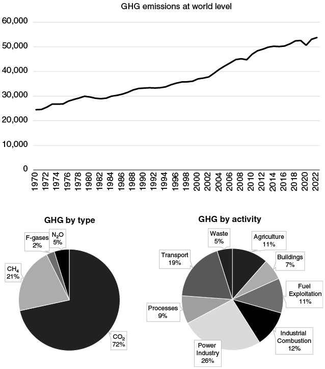
Human activities have profoundly affected Earth’s geology, landscape, limnology, ecosystems, and climate. The Anthropocene is a proposed geological epoch that dates from the commencement of significant human impact on Earth to the present day. The term Anthropocene combines anthropo (meaning man) and cene (meaning new). It highlights the mass extinctions of plant and animal species, ocean pollution, atmospheric alterations, and other lasting impacts caused by human activities. Human activities have significantly contributed to climate change through the emissions of GHG, deforestation, and other forms of environmental degradation. The burning of fossil fuels for energy production, transportation, and industrial processes is the largest source of anthropogenic GHG emissions, including carbon dioxide (CO2), methane (CH4), and nitrous oxide (N2O). Because human activities have emitted much more CO2 compared to any other gas, CO2 accounts for about three-quarters of GHG emissions of human origin. Methane emissions, which account around one-fifth of total GHG emissions, also offer key opportunities for emission reduction. These GHG emissions come from a variety of sources, the most important one being the combustion of fossil fuels (e.g., coal, oil, and gas) used to produce electricity for transportation and heating (Figure 1.1).
GHG emissions and by type

To make it comprehensive and easy to compare, the metric of global warming potential is widely used (Table 1.1). It measures how much greenhouse effect one tonne of the gas would create over 100 years compared to one tonne of CO2. For instance, methane emitted today is expected to stay in the atmosphere for only about a decade, much shorter than CO2. However, one molecule of methane has higher heat-trapping ability compared to one molecule of CO2. When we combine how long it stays in the atmosphere and how efficient it is at absorbing energy, we find that 1 tonne of methane is equivalent to more than 20 tonnes of CO2 in terms of the GHG effect.
| Greenhouse gas | Average lifetime in the atmosphere (years) | Global warming potential over 100 years (relative to CO2 = 1) |
|---|---|---|
| Carbon dioxide | 50–200 | 1 |
| Methane | 12 | 21 |
| Nitrous oxide | 120 | 310 |
| CFC-12 | 100 | 10,600 |
| CFC-11 | 45 | 4,600 |
| HFC-134a | 14.6 | 1,300 |
| Sulfur hexafluoride | 3,200 | 23,900 |
Other major sources of emissions are linked to industrial processes that are not combustion (e.g., cement production), as well as to agricultural activities and forest management. Deforestation and land use changes also release CO2 stored in forests and soils, further exacerbating global warming. This process is a large factor in emissions, as trees and plants remove CO2 from the atmosphere as they grow and convert it into carbon stored in the branches, leaves, trunks, roots, and soil. When forests are cleared or burnt, the stored carbon is released into the atmosphere, mainly as carbon dioxide. Additionally, intensive agriculture, livestock farming, and waste management practices produce methane and nitrous oxide emissions.
These human-induced changes to the Earth’s atmosphere have led to rising global temperatures, shifts in precipitation patterns, sea-level rise, and more frequent and intense extreme weather events. Addressing the root causes of climate change requires concerted efforts to reduce emissions, transition to renewable energy sources, promote sustainable land use practices, and adapt to the changing climate.
1.2.3 The Future of Climate Change
Climate experts project that global surface temperature will continue to increase until at least mid century under all global GHG emission scenarios. Global warming of 1.5°C and 2°C will be exceeded during the twenty-first century unless deep reductions in CO2 and other GHG emissions occur in the coming decades (IPCC, 2021). Scientific evidence shows that recent dramatic changes in climate systems can be widely attributed to human activities (IPCC, 2021). Since the mid nineteenth century, human influence has been behind the observed increase in the concentration of CO2 and other GHG, causing this unprecedented warming of the climate and change in global precipitation patterns. Human activities have also increased the frequency of compound extreme events since the 1950s, such as concurrent heat waves and droughts on a global scale. Climate scientists use climate models to simulate and reproduce the developments in the climate system. These models provide an accurate representation of the current state of the system only when considering human-induced emissions of GHG and human-induced changes in land use. If the effects of human activities are excluded, models fail to reproduce the current state of the climate system.
Scientists find that climate will continue to change in the future with overall higher temperatures and more intense and frequent extreme events, but also with irreversible changes in some systems. These future changes and risks remain highly uncertain, as they depend on the past but also on future emissions. These emissions, in turn, will be determined by human activity and adopted paths for socioeconomic and environmental policies. Climate scientists use models that represent Earth and human systems to explore these issues, and they use scenarios for the possible evolution of socioeconomic systems (e.g., technology, demography, economic growth, and land use) as well as the policies that would affect future emissions.
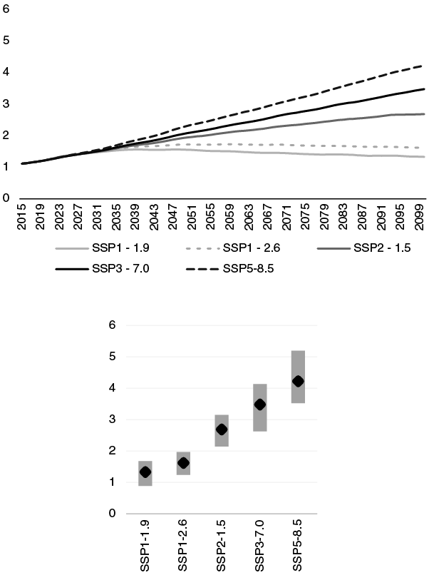
The IPCC scenarios below show diverse paths of evolution of global surface temperature under several scenarios. These scenarios are based on two main components: the shared socioeconomic pathways (SSP), which relate to the evolution of the economy and its demographics, and the representative concentration pathways (RCP), which represent the evolution of GHG in the atmosphere based on different policy choices impacting future emissions.
Five SSPs are envisaged:
SSP1 (low adaptation challenge, low mitigation challenge) describes a world characterized by strong international cooperation, prioritizing sustainable development;
SSP2 (medium adaptation challenge, medium mitigation challenge) describes a world where current trends continue;
SSP3 (high adaptation challenge, high mitigation challenge) depicts a fragmented world affected by competition between countries, slow economic growth, security-focused policies, and industrial production with little regard for the environment;
SSP4 (high adaptation challenge, low mitigation challenge) is a world marked by great inequalities between and within countries. In this scenario, a minority is responsible for the majority of GHG emissions, making mitigation policies easier to implement, while most of the population remains poor and vulnerable to climate change;
SSP5 (low adaptation challenge, high mitigation challenge) describes a world focused on traditional and rapid development in developing countries, based on high energy consumption and carbon-emitting technologies; the increase in living standards would enhance adaptation capacity, particularly by reducing extreme poverty.
The RCPs are scenarios that describe potential future changes in radiative forcing due to varying levels of GHG emissions. They are categorized by the radiative forcing level reached by the year 2100, expressed in watts per square meter (W/m²). The scenarios range from RCP 8.5, which represents high GHG concentrations and continuously increasing radiative forcing, to RCP 2.6, which describes a peak in emissions followed by a decline. The radiative forcing value for the year 2022 was 2.92 W/m² relative to 1750.
These scenarios serve as crucial tools for climate research and policy development, helping to assess the range of potential outcomes based on different socioeconomic and technological pathways. By combining these two types of scenarios, economists analyze climate change and its impacts on the economic system and climate. The scenarios span a spectrum of emissions levels, from low to high, reflecting a variety of future development choices and policy interventions. By exploring these scenarios, scientists and policymakers gain insights into possible climate futures and the corresponding risks and opportunities for adaptation and mitigation. The socioeconomic dynamics, such as technology choices, investment, and policy decisions of today, will alter emissions and impact climate change in the future. Depending on these scenarios for the future, we see that the warming in 2100 can possibly range between 1.5°C and almost 5°C (Figure 1.2).
Global surface temperature change relative to 1850–1900 (in °C) in IPCC scenarios
Note: Projected median warming across global modeled pathways (top panel) and 5–95% 2,100 temperature outcomes – median as diamond – (bottom panel) for the five illustrative scenarios (SSPx-y).

These overall average temperatures entail significant variations at the local level. For instance, warming is predicted to be more pronounced in higher latitudes and continents and less intense in the tropics and oceans. The same heterogeneity is expected for precipitations, global warming is set to cause more rainfall on average but in high latitudes and during the winter. Conversely, less rainfall is projected in the tropics and during the summer. All in all, the average temperature increase will exacerbate existing climate vulnerabilities, such as water scarcity or excess water, in the future.
1.2.4 Irreversibility and Tipping Points
Recent research shows that in response to CO2 emissions, some regions of the world might experience irreversible climate change. This implies that even after removing emissions, the impact of emissions could last in some regions (Kim, S.-K. et al., Reference Kim, Shin and An2022). Widespread irreversible changes in atmospheric variables could also induce irreversible changes in other subcomponents of the Earth’s systems, such as mountain glaciers, sea ice, and rainforests. These climate irreversibility hotspots are mostly identified in coastal regions covered with ice, such as Antarctica, Greenland, Alaska, and the high mountain glacier region of the Himalayas, as well as monsoon areas, such as the African and South American monsoon regions.
Climate tipping points refer to the nonlinear response of extreme events to small changes in the climate. When the tipping points are reached, small changes may become significant enough to cause a larger, more critical change that can be abrupt, irreversible, and lead to cascading effects. The tipping points can create compound risks to natural and human systems. Overshooting the Paris Agreement warming targets would increase the risk of hitting tipping points and triggering irreversible changes in the system, like permafrost thawing or dieback of the Amazon rainforest. Triggering this tipping point would make it a lot more difficult, if not impossible, to get back below the 1.5°C target. The Greenland ice sheet, on the other hand, contains enough water to raise global sea levels by over 20 feet. Its melting has significantly accelerated since the 1990s and could reach a critical point beyond which its eventual collapse is irreversible for millennia.
Each small change in the average climate, temperatures, and precipitations causes major changes in the frequency and severity of the climate extremes. When we take the example of heat waves, an episode that occurred once every fifty years in the nineteenth century occurs five times more frequently today with +1°C of warming. In the case of the scenario with +1.5°C of warming, the event that occurred once in fifty years is expected to become common, occurring every five years (nine times more frequently). Considering the 4°C warming scenario, the frequency increases forty times. The heat waves that happened in the past once every fifty years would occur almost every year.
Deep uncertainty exists with regard to the biogeochemical processes potentially triggered by climate change. Climate scientists have shown not only that tipping points exist but remain difficult to estimate with precision, but also that they could generate tipping cascades on other biogeochemical processes. Evidence is now mounting that tipping points in the Earth system, such as the loss of the Amazon forest or the West Antarctic ice sheet, could occur more rapidly than was thought (Lenton et al., Reference Lenton, Rockström and Gaffney2019).
Some research has proven the existence of a planetary threshold in the trajectory of the Earth System that, if crossed, could prevent stabilization in a range of intermediate temperature rises. The Late Quaternary (past 1.2 million years) has seen an alternation between glacial (cold) and interglacial (warm) periods. These cycles, known as Milankovitch cycles, are driven by changes in Earth’s orbit and axial tilt. Not every cycle follows the same trajectory, but they share an overall pathway. The full glacial and interglacial states, along with approximately 100,000-year oscillations between them, constitute limit cycles. The Anthropocene marks a pivotal moment in Earth’s history – a departure from the familiar glacial-interglacial cycles toward a new trajectory shaped by human influence. It represents a rapid shift away from the natural glacial-interglacial rhythm propelled by human activities. Currently, over 1°C above preindustrial temperatures, the Earth is approaching the upper limit of interglacial conditions in the past 1.2 million years. Over the past half-century, our climate system has followed an accelerated path, and the Earth System may have already passed a critical juncture – a bifurcation – leading away from the next glaciation cycle (Ganopolski et al., Reference Ganopolski, Winkelmann and Schellnhuber2016).
In contemplating the Earth’s future, we encounter a multitude of potential trajectories. These pathways, often depicted by climate models, span a wide range of global temperature increases. Traditionally, these trajectories correlate closely with cumulative GHG – particularly carbon dioxide – released by human activities. However, beyond straightforward emissions, the Earth System’s fate is influenced by intricate biogeophysical feedback, and these processes involve interactions between living organisms, land, oceans, and the atmosphere. They can amplify or dampen climate effects, affecting the overall trajectory. Steffen et al. (Reference Steffen, Rockström and Richardson2018) claim that there is a significant risk that these dynamics, especially strong nonlinearities in feedback processes, could become a dominant factor in steering the trajectory that the Earth System actually follows over the coming centuries.
Physical climate risks may be far greater in magnitude and materialize much sooner than previously anticipated. The Earth is currently on a trajectory toward a Hot house Earth state with potentially irreversible impacts. This could be further accelerated by tipping points such as the loss of ice sheets, rainforest cover, and permafrost. Tipping elements in our planet’s complex system can behave quite differently, showing abrupt shifts, when they cross their critical thresholds. For instance, the Amazon rainforest could suddenly convert to a savanna or a seasonally dry forest. This type of change could occur rapidly and dramatically. Other elements respond more gradually but persistently, like the large-scale loss of permafrost, which, once started, tends to continue. Such a gradual shift can have long-lasting effects.
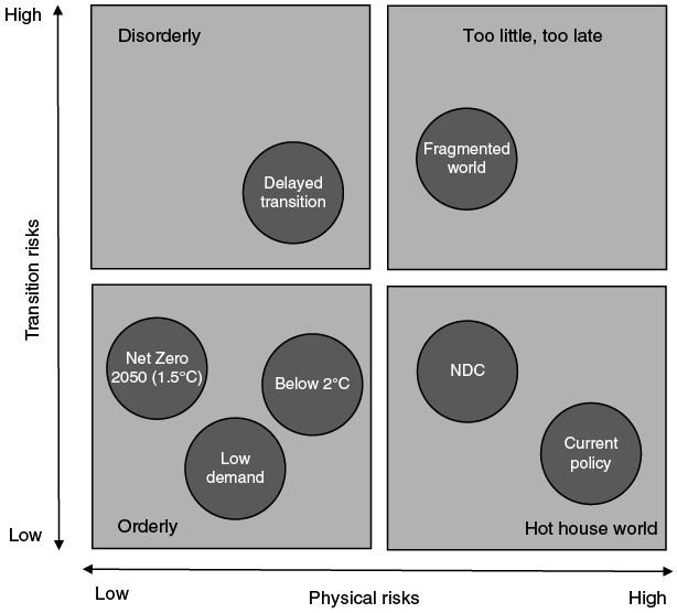
1.2.5 Macroeconomic and Financial Scenarios
The IPCC scenarios that were referred to earlier focus on overall possible future trends in physical and socioeconomic pathways. Based on such analysis, the Network for Greening the Financial System (NGFS), a coalition of central banks and supervisory authorities,Footnote 2 has developed a set of reference scenarios to assess the impact of climate risks on a wide-ranging set of economic and financial variables (e.g., GDP, inflation, equity and bond prices, and loan valuations). The NGFS regularly publishes several reference scenarios characterizing four different situations (see Figure 1.3). The first family of scenarios refers to an orderly transition. In these scenarios, the transition begins immediately with the introduction of proactive mitigation policies, such as a carbon tax policy or measures to support renewable energies. It is also based on assumptions of transformations in the behavior of consumers and financial players, better aligned with the requirements of a low-carbon economy. Announced and anticipated, this structural transformation of the economy is taking place gradually and without major macroeconomic shocks. Compliance with climate commitments also reduces physical risks. The second family of scenarios describes the response to a disorderly transition, which may be delayed or sudden, in both cases insufficiently anticipated and therefore abrupt. In the case of a delayed transition, new, more restrictive measures may, for example, be introduced, resulting in more disruptive adjustments depending on the sector. Households and businesses would then have to adjust their behavior rapidly, leading to major macroeconomic and sectoral disruptions. On the other hand, meeting climate targets limits physical risks. The third family of scenarios, Hot house world, corresponds to Business as usual. In this scenario, governments do not introduce any transition measures other than those already in place, and economic players do not change their behavior. GHG emissions, therefore, continue on past trends, causing temperatures to rise above 2°C, worsening chronic physical risks, and increasing the frequency and severity of extreme weather events. On the other hand, the risks of transition remain limited. Finally, the last family corresponds to too-little, too-late scenarios where mitigation actions remain insufficient to achieve temperature objectives, and the materialization of physical risk leads to a disorderly transition.
NGFS scenarios

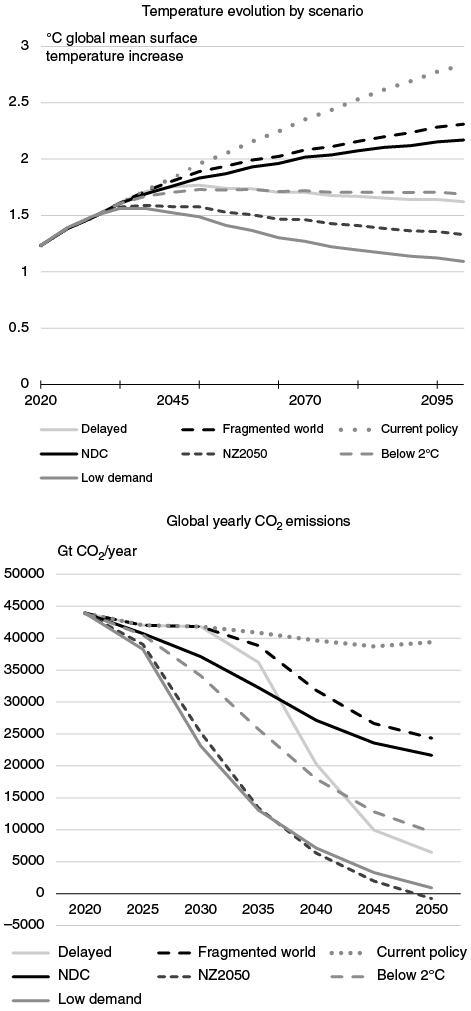
In the NGFS scenarios where climate goals are met, deep reductions in emissions are required to limit the rise in global mean temperatures to below 1.5°C or 2°C by the end of the century (Figure 1.3). This does not occur in the Current policies scenario, leading to a temperature rise exceeding 3°C and severe and irreversible impacts. Temperatures are increasing unevenly across the world with land warming faster than oceans and high latitudes experiencing higher warming. Temperature changes lead to chronic changes in living conditions affecting health, labor productivity, agriculture, ecosystems, and sea-level rise. It is also changing the frequency and severity of weather events such as heat waves, droughts, wildfires, tropical cyclones, and flooding.
1.2.6 Why Is Scenario Analysis So Important for Climate Economics and Finance?
The unique features of climate risks present a hurdle to traditional risk assessment methods. Climate risks unfold over extended timeframes accompanied by significant uncertainty regarding policy trajectory and socioeconomic influences. They manifest globally and across economies, with varying complexity across regions and industries. These distinctive attributes elude conventional risk assessment approaches, which rely on simplistic modeling and historical data, narrow scopes, and assumptions of static economic and financial structures. Scenario analysis emerges, therefore, as a crucial solution to address these challenges. It offers a dynamic framework for exploring potential future trajectories, allowing stakeholders to better grasp how climate-related factors may shape economic and financial landscapes. This tool proves, in particular, invaluable for central banks, supervisors, financial entities, businesses, and policymakers seeking deeper insights into the impact of climate dynamics.
A scenario is a description of a possible future, encompassing both quantitative and qualitative elements (Foster, Reference Foster1993). Such a description requires “a story with plausible cause and effect links that connects a future condition with the present, while illustrating key decisions, events, and consequences throughout the narrative” (Glenn, Reference Glenn2009). Scenarios are not predictions but reflect experts’ knowledge about probable future outcomes based on “internally consistent and challenging narrative descriptions of possible futures” (van der Heijden, Reference Van der Heijden2005). In the case of climate scenarios, each individual narrative is, therefore, an alternative description of how the future may unfold associated with a combination of socioeconomic, policy, technological, and climate changes (Mallampalli et al., Reference Mallampalli, Mavrommati and Thompson2016) and their impact on the future state of the key climate and economic and financial variables.
Climate scenarios first require the specification of the time horizon, either short to span frequencies relevant to central banks and supervisors, that is, between 3 and 5 years, or long to describe structural changes that an economy could undertake and the climate impacts associated, that is, 50 or 100 years. Each narrative is based on selected key drivers, which can be either a policy decision (mitigation policy or adaptation), a change in economic agents’ behavior (e.g., repricing of risks by financial investors and increased savings by households facing higher uncertainty), or a technological change (e.g., innovation in green technologies that fosters productivity).
Although primarily qualitative, the scenario description can also provide insights into the severity of events. For example, the assumption that a scenario remains consistent with climate targets induces some degree of policy action; conversely, deviating from climate targets affects the potential severity of weather events. Relying on multiple scenarios reflects not only the trade-off between transition and physical risks but also the different nature of the key drivers, some of which primarily affect the supply side of the economy (e.g., carbon taxation or technological innovation), while others may be associated with demand-side drivers (e.g., public spending on green infrastructures or reduced consumption due to uncertainty in transition policies). Such diversity covers multiple use cases and provides a range of macrofinancial outcomes that can be useful in assessing the macroeconomic and financial stability implications of climate-related risks.
Finally, it is worth noting that adopting climate-related scenario analysis remains nascent, with methodologies in a continual state of refinement. Key challenges include the incomplete amalgamation of physical risk, transition risk, and macrofinancial transmission channels; scarcity of accessible data and research to fine-tune scenarios and evaluate repercussions; and a deficiency in technical proficiency concerning climate science and environmental economics within the financial domain.
1.3 Assessing the Economic Impacts of Climate Change
As per our understanding of science progresses and we collectively witness the rise in extreme weather events and other climate-related phenomena, the dangers posed by climate change become increasingly apparent. For businesses, the repercussions of this changing climate can manifest in financial losses – through property damage and other asset depreciation, as well as disruptions to operations, supply chains, and the broader social and economic frameworks businesses rely on.
The escalating frequency and/or severity of climate-related hazards – including those related to temperature, water, oceans, land, and wind – are already inflicting financial harm. After briefly reviewing historical trends in climate-related disasters, we will provide a typology of climate-related shocks that can weigh on economic and financial systems. We will then analyze the different transmission channels of those shocks before presenting various methodologies to assess their effects on economic growth and welfare.
1.3.1 Historical Trends in the Frequency and Cost of Climate-Related Disasters
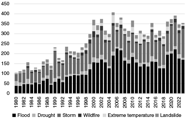
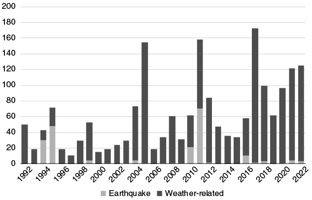
Data on climate-related disasters are difficult to collect. The International Disaster Database (EM-DAT, www.emdat.be/) stands out as the only freely available global disaster loss database, but its effectiveness is limited by a narrow pool of sources and gaps in reporting accuracy. Despite these shortcomings, EM-DAT remains an indispensable tool for understanding disaster occurrences and impacts. Figure 1.4 shows the increase in the frequency of events since 1980, broken down into different perils. Floods and storms represent the larger share of disasters, and their frequency has clearly increased over the last forty years. The number of events has been multiplied by 3–4 since 1980.
Frequency of natural disasters (number of disasters per year)

In terms of losses, reinsurers assess global costs every year. Munich Re – the world’s largest reinsurer – has released its global disaster loss calculation for 2023, coming in at a total of USD 250 billion. This roughly equals the entire GDP of New Zealand or Portugal. It is also slightly lower than the previous estimate for 2022, which originally came in at USD 270 billion. For Swiss Re, in 2023, natural catastrophes resulted in economic losses of USD 280 billion, for 332 catastrophe events and 76,000 victims. Out of the USD 280 billion of total loss, USD 108 billion was insured. Insured losses (Figure 1.5) also increased over the last fifty years, and a clear upward trend is noticeable. Most of the losses are weather-related. These assessments offer only a fragmented view of the genuine magnitude of disasters, encompassing human casualties and economic, developmental, and social consequences. Many repercussions of disasters go unaccounted for in these evaluations. These include effects linked to gradual-onset and localized incidents, as well as the cascading consequences of disrupted supply chains, diminished productivity, compromised physical and mental well-being, and lasting disruptions to education. Together, these factors contribute to an unseen toll of disasters that far surpasses the economic estimates provided by insurers.
Growth in global natural catastrophe insured losses (2022 USD billion)
North America emerges as the region with the most significant economic repercussions, representing around 40 percent of the global losses. Typically, wealthier nations bear the brunt of financial losses from disasters due to their larger stock of more high-value assets, which are often insured. However, lower-income countries shoulder a disproportionate economic burden relative to their overall wealth. While absolute dollar losses are higher in high-income nations, low-income and lower-middle-income countries record a notably larger share of economic loss compared to the global average. Additionally, poorer countries endure the most significant tolls in terms of both lives lost and disruptions experienced.
Furthermore, there exists a bias toward major events that receive widespread coverage, whereas lesser-known incidents, although infrequently reported, accumulate substantial losses. Table 1.2 includes the top twenty costliest climate-related events. Most of them were taking place in North America (US and Canada). Among the developing nations, Caribbean and South/Southeast Asian countries are the most exposed to severe disasters.
| Event | Type | Year | Location | Financial losses (in billions USD) |
|---|---|---|---|---|
| Hurricane Katrina | Tropical cyclone | 2005 | United States | $125 |
| Hurricane Harvey | Tropical cyclone | 2017 | United States | $125 |
| Hurricane Ian | Tropical cyclone | 2022 | North America (United States, Cuba, Venezuela) | $113 |
| 2020 South Asian floods | Flood | 2020 | South Asia (India, Pakistan, Bangladesh) | $105 |
| Hurricane Maria | Tropical cyclone | 2017 | North America (Puerto Rico, Dominica, Guadeloupe) | $91.6 |
| Hurricane Ida | Tropical cyclone | 2021 | North America (United States, Cuba, Venezuela) | $75 |
| 2019–2020 Australian bushfires | Wildfire | 2019–20 | Australia | $70 |
| Hurricane Sandy | Tropical cyclone | 2012 | North America (United States, Haiti, Cuba) | $68.7 |
| Hurricane Irma | Tropical cyclone | 2017 | North America (United States, Sint Maarten, etc.) | $64.8 |
| 1988–1990 North American drought | Drought | 1988–89 | United States, Canada | $53.25 |
| 2012–2013 North American drought | Drought | 2012–13 | United States, Canada | $49.6–$56.1 |
| 2011 Thailand floods | Flood | 2011 | Thailand | $45.7 |
| 2022 Pakistan floods | Flood | 2022 | Pakistan | $40 |
| Hurricane Ike | Tropical cyclone | 2008 | North America (United States, Haiti, Cuba) | $38 |
| 2020 China floods | Flood | 2020 | China | $32 |
| Typhoon Doksuri | Tropical cyclone | 2023 | Southeast Asia (China, Philippines, Taiwan, etc.) | $28.4 |
| Hurricane Wilma | Tropical cyclone | 2005 | North America (United States, Mexico, Haiti, etc.) | $27.4 |
| Hurricane Andrew | Tropical cyclone | 1992 | United States | $27.3 |
| February 13–17, 2021 North American winter storm | Winter storm, Infrastructure failure (electric) | 2021 | North America (United States, Mexico, Canada) | $26.5 |
| Hurricane Ivan | Tropical cyclone | 2004 | North America (United States, Grenada, Jamaica, etc.) | $26.1 |
Although data collection extends beyond insurance companies (municipalities, national governments, international organizations, and nongovernmental organizations), these datasets often lack comparability and may reflect inherent biases due to variations in collection methods and intended uses. For instance, recording a higher number of victims might influence aid allocation, while a lower count could mitigate authorities’ accountability.
Overall, the complexities involved in recording, reporting, and compiling data on disaster impacts frequently yield fragmented, disjointed, or incomplete datasets, particularly within globally comprehensive databases (see UNDRR, 2023).
1.3.2 Climate Change, Weather, and Disasters
Up to this point, we have referred to the physical consequences of global warming in general terms – through climate change, weather conditions, and disaster frequency. To assess the economic consequences of such a complex phenomena, we need first to provide a clear terminology.
1.3.2.1 Climate
Climate refers to the long-term average of weather conditions in a specific region over an extended period (usually thirty years or more). It is characterized by the following:
Stability: Climate is relatively stable and predictable over time.
Patterns: It encompasses patterns of temperature, humidity, wind, precipitation, and other atmospheric conditions.
Influence: Climate is influenced by factors such as latitude, altitude, ocean currents, and GHG concentrations.
Example: The tropical rainforest climate in the Amazon basin has high temperatures, heavy rainfall, and consistent humidity year-round.
1.3.2.2 Weather
Weather refers to the short-term atmospheric conditions (usually over hours to a few days) in a specific location. It is characterized by the following:
Variability: Weather can change rapidly and is often unpredictable.
Elements: It includes elements such as temperature, humidity, wind speed, cloud cover, and precipitation.
Influence: Weather is influenced by local factors, such as air pressure systems, fronts, and seasonal variations.
Example: On May 6, 2024, BBC weather forecasts: “Tomorrow morning will be largely dry with plenty of sunshine. Variable cloud and a few scattered showers will develop through the afternoon, these largely dying out by evening.”
1.3.2.3 Natural Hazards
These are extreme events caused by natural processes that can potentially result in significant harm to human life, property, and the environment. They are characterized by the following:
Severity: These events are severe and have catastrophic consequences when they hit human communities.
Types: Natural hazards include earthquakes, hurricanes, floods, droughts, wildfires, and volcanic eruptions.
Impact: They can lead to loss of life, displacement, economic damage, and environmental degradation.
Example: In 2011, Thailand experienced its worst flooding in years, leaving more than 800 people dead and causing severe damage across.
The term natural disaster is commonly used to describe catastrophic events such as hurricanes, floods, earthquakes, or volcanic eruptions. However, this term can be misleading as it masks the role of human decisions and vulnerabilities. We prefer using the term natural hazard, which denotes a naturally occurring event such as earthquakes, hurricanes, or floods, capable of endangering human life, property, and the environment. As we focus only on weather-related events, we will therefore use weather-related hazards/extreme events. While the term hazard signifies the inherent risk associated with such phenomena, a natural disaster arises when a hazard materializes, resulting in notable damage, destruction, and loss. While a hazard presents a potential danger, a disaster represents its actual occurrence, underscoring widespread devastation and the imperative for response, recovery, and reconstruction efforts. In that sense, the adjective natural may be misleading because, while these phenomena stem from natural forces, their societal impact is deeply intertwined with human factors such as urbanization and infrastructure development. Categorizing such occurrences as natural can foster a perception of inevitability, overlooking the influence of societal choices on disaster risk.
In summary, climate represents long-term patterns, weather describes short-term conditions, and natural hazards are extreme events with potentially significant impacts. In what follows, we will distinguish physical risks into two broad categories:
Chronic risks due to gradual global warming and the associated physical changes, such as rising sea levels or changing precipitation patterns; and
Acute risks due to extreme weather events, such as tropical cyclones, storms, floods, and drought.
Though different in timing and immediate severity, both risks are dynamic, evolving over time and interacting with each other in a complex and nonlinear fashion.
1.3.3 Channels of Transmission to the Economy
The comprehensive examination presented in Table 1.3 provides a nuanced exploration of the multiple impacts of both chronic risks (gradual warming) and acute risks (extreme events) on the intricate structure of the economy. As temperatures steadily rise and climate patterns shift, the impacts are widespread and complex, permeating every facet of economic activity. From the agricultural sector grappling with declining yields and productivity losses due to changing climatic conditions, to labor markets facing disruptions from extreme heat waves and shifts in migration patterns, the effects of gradual warming are widespread and profound.
| Channels of impact | Chronic risks (gradual warming) | Acute risks (extreme events) |
|---|---|---|
| Food, energy and other input supply | Decline in agriculture productivity and yields. | Disruption to transport and production chains. |
| Labor supply | Loss of hours worked due to extreme temperatures. Increased international migration. | Destruction of workplaces, need to migrate (even if temporarily). |
| Capital stock | Diversion of resources from productive investment to adaptation capital. | Destruction due to extreme events. |
| Technology | Diversion of resources to reconstruction activity. | Diversion of resources to reconstruction activity. |
| Productivity | Lower labor productivity due to extreme heat waves and lower human capital accumulation (increased health issues and mortality). | Lower capital productivity due to (possibly permanent) capital and infrastructure destruction. |
| Energy demand | Increased demand for electricity in summer exceeds decreased demand in winter. Higher carbon tax leading to lower demand for fossil fuels. | Change in preferences toward more sustainable goods and services. |
| Investment | Change in preferences toward more sustainable goods and services. Uncertainty about climate events could delay investment. | Investment in reconstruction increases following events. |
| Consumption | Change in preferences toward more sustainable goods and services. If no insurance of household or firms, destruction could cause a permanent decrease in wealth and affect consumption. | Increased sustainability awareness and a shift toward greener consumption. |
| Trade | Disruption to trade routes due to geophysical changes (such as rising sea levels). Change in food prices and disruption to trade flows. | Risks of distortion from asymmetric or unilateral climate policies. |
| Aggregate Impact on Output | Lower labor productivity, investment being diverted to mitigation and arable land loss. | Physical destruction (crop failures, destruction of facilities and infrastructure, disruption of supply chains). |
| Wages | Downward pressures on wages from lower productivity. Unequal effects across sectors and economies. | Unequal effects across sectors and economies (reallocation of workers from one sector to another, increased training needs). |
| Inflation | Relative price changes due to shifting consumer demand or preferences and changes in comparative cost advantages. | Increased inflation volatility, particularly in food, housing, and energy prices. |
| Inflation Expectations | Climate-related shocks, for example, to food and energy prices, may affect inflation expectations. Inducing more homogeneous, sudden, and frequent revisions of expectations. | Formation of inflation expectations affected by policies. |
Global warming affects both the supply and demand sides of the macroeconomy. Concerning supply shocks, labor availability, and productivity might decrease due to factors such as heat stress, migration, and temporary incapacitation to work. The capital stock may diminish and undergo changes due to resource reallocation for adaptation purposes, while technology could suffer from diverted resources away from innovation and research toward reconstruction and adaptation efforts. This could lead to a slowdown in productivity growth, affecting future incomes and calling for higher savings to maintain future consumption levels. On the demand side, changes in energy demand may result from anticipated shifts in energy prices and consumer preferences. Additionally, investment dynamics may weaken due to increased uncertainty, although there could be a temporary boost in investment related to reconstruction needs. Changes in consumption patterns may emerge from shifts in preferences, increased precautionary savings, and enduring wealth losses for uninsured individuals.
At the same time, the looming threat of extreme events is becoming increasingly evident, heralding widespread devastation and upheaval in infrastructure networks, supply chains, and production systems. Hurricanes, floods, and wildfires leave a trail of destruction in their wake, compelling urgent efforts to rebuild and adapt while reshaping consumer preferences and investment strategies.
Similar to global warming, extreme weather events impact both the supply and demand sides of the economy. However, these effects vary in terms of timing and severity compared to those induced by global warming (as outlined in Table 1.3). Extreme weather events prompt immediate and significant economic repercussions on the supply side, damaging workplaces, depleting productive capital, disrupting production processes, impeding energy supply, and disrupting global value chains. Trade may also suffer due to disruptions in transportation links and shifts in relative prices. These macroeconomic impacts pose challenges for central banks in the short term, as they often lead to conflicting trends in output and inflation (see Chapter 5). As for demand side impacts, investment may stagnate due to heightened uncertainty, although short-term boosts may occur from reconstruction efforts. Consumption may suffer if uninsured agents face permanent wealth losses.
The consequences of these climate-related phenomena reverberate through the economy, triggering cascading effects across multiple dimensions. Capital investment is redirected toward resilience-building measures and infrastructure upgrades, while shifts in consumer demand force industries to adapt and innovate. Trade dynamics are reshaped as disruptions to global supply chains alter production and consumption patterns, creating both winners and losers in the global marketplace (Andersson et al., Reference Andersson, Baccianti and Morgan2020).
Table 1.3 also highlights the inherent disparities and inequalities that underpin the distribution of climate risks and impacts. Vulnerable communities, particularly those in low-income regions and developing countries, bear a disproportionate burden of climate-related shocks and face increased risks of displacement, economic hardship, and social upheaval.
1.3.4 Measuring the Economic Impacts of Physical Risks
Traditionally, climate impact studies adopt a top-down approach, where different scenarios of GHG concentrations are simulated using Earth system models to provide broad-scale projections. Hydroclimatic variables relevant to specific hazards, such as floods or wildfires, are often downscaled either statistically or dynamically to match the spatiotemporal scale of these processes. Subsequently, societal impacts, characterized by losses pertinent to stakeholders, are determined based on the hazard, incorporating additional factors related to impact exposure and vulnerability. This assessment informs decision-making processes. Recently, there has been increasing interest in stakeholder-centered approaches, or bottom-up approaches. These approaches employ risk-based reasoning, beginning with an understanding of stakeholders’ information needs, including key decision-making criteria, decision variable nature, impact domain, and spatial and temporal scales of climate and meteorological processes (Leonard et al., Reference Leonard, Westra and Phatak2014).
The various hazards do not have the same scale, neither in terms of distance nor in terms of time. At the micro-scale (<2 km), numerous events occur, including lightning strikes initiating wildfires, wind eddies, hailstone, and rainfall formation. Within the 2–20 km range, thermal convection can lead to intense rainfall bursts, flash flooding, strong winds, or tornadoes. Cold fronts within the 20–200-km scale can generate individual or sequences of storm events lasting hours to days. Events spanning multiple days are often associated with synoptic weather patterns such as tropical cyclones and anti-cyclones (e.g., wildfires and heat waves). Natural climatic variability may induce periods of above or below-average occurrence rates of extreme events over years or decades. Ultimately, anthropogenic climate change may drive long-term trends such as increased temperatures or ocean levels, expected to unfold over centuries or longer (Leonard et al., Reference Leonard, Westra and Phatak2014).
In this section, we will briefly review how weather-related hazards need to be assessed together with exposure and vulnerability to correctly assess risks. We will then look at bottom-up approaches, introducing the concept of damage function for each climate-related hazard, before presenting the aggregate damage functions used in top-down approaches.
1.3.4.1 Hazards, Exposure, and Vulnerability
The impact of climate and weather-related events on individuals and economic systems is shaped by hazard, exposure, and vulnerability (Figure 1.6). The hazard represents the likelihood of an extreme weather event occurring, exposure identifies the individuals or assets that could be impacted by the weather event, and vulnerability assesses the extent to which these individuals or assets may suffer adverse consequences. More precisely (IPCC, 2012):
Hazard: The potential occurrence of a climate or weather-related event or trend that may cause loss of life, injury, or other health impacts, as well as damages and loss to property, infrastructure, livelihoods, service provision, ecosystems, and environmental resources.
Exposure: The presence of people, livelihoods, species or ecosystems, environmental functions, services, and resources, and infrastructure. These, together with economic, social, or cultural assets, may be found in places and settings that could be adversely affected.
Vulnerability: The propensity or predisposition to be adversely affected. Vulnerability encompasses a variety of concepts and elements, including sensitivity or susceptibility to harm and lack of capacity to cope and adapt.
The articulation between hazards, exposure, and vulnerability
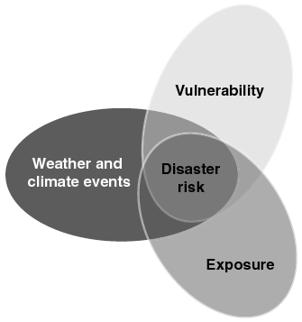
When modeling risks, these three dimensions should be taken into account. The unit chosen to measure risk should be the most pertinent in a given decision context, which may not necessarily be monetary units. For instance, wildfire hazard could be quantified by burned area, exposure by population, and risk expressed as the number of affected individuals for evacuation planning or the repair cost of buildings for property insurance purposes. Risk, as defined by the International Organization for Standardization and the IPCC, reflects the potential for consequences when uncertainty surrounds objectives or values. It can be quantified by combining the probability of an outcome with its magnitude, often represented by a convolution of probability and severity distributions.
1.3.4.2 Damage Functions for Climate-Related Hazards
Damage functions are utilized in climate or weather-related hazard risk assessments to convert the severity of extreme events into measurable damage. A damage function is defined as the mathematical relation between the magnitude of a (natural) hazard and the average damage caused either on a single structure (microscale), for example, a building, or a portfolio of structures (macroscale). The emphasis is on direct monetary damage, but the findings can be generalized to any measurable quantity (Prahl et al., Reference Prahl, Rybski and Burghoff2015, Reference Prahl, Rybski and Boettle2016). Microscale models can be empirical (i.e., statistically derived from data), engineering-based, or a mixture of both. On the macroscale, damages may be either aggregated from microscale models or obtained from statistical relationships based on empirical data (Merz et al., Reference Merz, Kreibich and Schwarze2010).
We provide here two examples of damage functions at the macroscale that relate to the hazards of coastal flooding and wind storms.
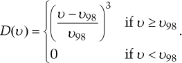
1.3.4.2.1 Coastal Flooding
The analysis requires a detailed mapping of the geographical areas that could have possibly been flooded and the buildings affected. For example, Boettle et al. (Reference Boettle, Kropp and Reiber2011) concentrate on a hypothetical storm surge occurrence in an area in Denmark, presuming that the seawater entirely submerges the landscape at the specified water level. To pinpoint the submerged area, they utilize a map incorporating elevation data, delineating areas susceptible to inundation with high precision. Subsequently, they ascertain which properties fall within the inundated zone and compute the extent of flooding for each building.
A diverse array of functional forms, including logarithmic, square-root, linear, and quadratic models (see Nascimento et al., Reference Nascimento, Machado and Baptista2007; Dutta et al., Reference Dutta, Herath and Musiake2003; Buchele et al., Reference Buchele, Kreibich and Kron2006; Apel et al., Reference Apel, Aronica and Kreibich2009, and related literature) have been employed as building damage functions for flooding risks. Boettle et al. (Reference Boettle, Kropp and Reiber2011) opt for a linear function represented as:

where e signifies the water level relative to the building’s foundation base. This function is applied to all affected buildings, and the aggregate damage for the specified sea-level E is computed as follows:

where ei represents the flood height at building i and Vi denotes its value. D(E) can be interpreted as an approximation of the total monetary damage incurred by a particular flood event of magnitude E affecting buildings across the entire study area. Adjusting the sea-level E in increments of 10 cm from 0 m to 3 m establishes a macroscopic damage function with zero loss up to 1 m and exponentially increases up to 400 million Danish krona when water reaches 3 m.
1.3.4.2.2 Wind Storms
Klawa and Ulbrich (Reference Klawa and Ulbrich2003) developed a simple storm damage function based on a cubic power law term as a proxy for storm damage (Prahl et al., Reference Prahl, Rybski and Burghoff2015).
The shape of the damage function is determined by the power law term, which is influenced only by the 98th wind gust percentile. The value of this threshold controls the shape and the steepness of the damage function. Leckebusch et al. (Reference Leckebusch, Ulbrich and Fröhlich2007) amend this function by noting that damages depend on the amount of values in an affected area, and the population density (p) is used as a reasonable proxy. Thus, the applied damage function is given by the following:
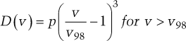
Storm-damage functions are typically calibrated to insurance data. Jaison (Reference Jaison, Sorteberg and Michel2023) uses different damage functions, including the excess cubic one as detailed above, to assess windstorm damages for Norway using municipality-level insurance data and the high-resolution wind speed data for the period 1985–2020. Here again, there is no loss as long as wind speed is lower than 12 m/s and then losses increase up to 400 Norwegian krona/person when it is higher than 18 m/s.
Overall, empirical damage functions are generally challenging to derive due to insufficient observations for certain impacts or locations. Moreover, weak correlations between loss and explanatory variables could render loss estimates unreliable, amplifying uncertainty. This underscores the necessity for a comprehensive damage assessment to facilitate the quantification and comparison of impacts across different natural hazards and their interrelations (Kreibich et al., Reference Kreibich, Bubeck and Kunz2014).
1.3.4.3 Aggregate Climate Damage Functions
Bottom-up damage functions are used in catastrophe models of the insurance sector to correctly assess the risk of losses they could be exposed to. They are limited, however, to direct impacts, that is, the immediate harm inflicted upon assets (e.g., property) by a weather-related event, resulting in losses occurring either during or shortly after the event. However, the economic effects of physical risks should also include indirect impacts, which encompass alterations in economic activity post-disaster. These effects cover disruptions in economic operations and any positive repercussions stemming from production substitution and reconstruction demand. Indirect impacts encapsulate both short- and long-term economic setbacks in production and consumption, along with related pathways to economic recovery (Kousky, Reference Kousky2014). These indirect repercussions, sometimes referred to as higher-order effects, can be quantified through computational macroeconomic models. Such forecasts are subject to empirical validation, employing diverse economic indicators such as gross domestic product (GDP), trade patterns, and employment figures (Botzen et al., Reference Botzen, Deschenes and Sanders2019).
Aggregate damage functions are defined to assess from a top-down perspective how changes in climate or weather can imply economic impacts. A climate damage function is, therefore, a simplified expression of economic damages (which theoretically can encompass both positive and negative effects) as a function of climate inputs, such as changes in temperature (Neuman et al., Reference Neumann, Willwerth and Martinich2020).
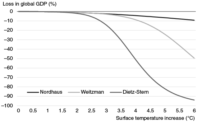
1.3.4.3.1 Nordhaus; Weitzman; Dietz and Stern
Climate damage functions assess the economic risks posed by climate change, quantifying the impact on the economy. Economic climate damage is defined as the proportionate reduction in annual economic output at a specific degree of warming compared to output in the absence of warming. These functions illustrate the decline in output across various warming scenarios, with all indicating greater output loss as temperatures rise. However, consensus is lacking among estimated climate damage functions regarding the progression of damages with incremental warming. We present here the three most influential damage functions of the literature, their specifications, and their implications in terms of losses.
Nordhaus (Reference Nordhaus2018) includes a damage function in his Integrated Assessment Model, DICE (see more details in Chapter 2), which has the following specifications:
 (1.1)
(1.1)
With  representing one minus the fraction of aggregate output (in trillion USD) lost due to climate change.
In the above equations, t is time (decades in DICE) and  is the global mean surface temperature. For a zero temperature change
  (no damage) and for very large temperature changes it approaches 0 (maximum damage). The DICE damage function is calibrated to damages in the range of 2°C–4°C.
Other economists have proposed more convex functions, notably Weitzman (Reference Weitzman2010) and Dietz and Stern (Reference Dietz and Stern2015).
Weitzman (Reference Weitzman2010) proposes an alternative damage function, namely,
 ((1.2))
This establishes a tipping point at which the damage function illustrates significant impacts once the temperature rises beyond 6°C. At this juncture, the specification indicates approximately a 50 percent damage threshold. Weitzman supports this by citing an expert panel study involving fifty-two experts, which suggests that at this temperature increase, three out of five critical tipping points for major climate change events or scenarios are anticipated to emerge.
Dietz and Stern (Reference Dietz and Stern2015) modify the Weitzman-based function by different parameters:
 (1.3)
(1.3)In addition to a different functional specification for the damage function itself, Dietz and Stern (Reference Dietz and Stern2015) also consider the effects of damages to capital and to TFP, instead of damages to output only.
Figure 1.7 illustrates the different behaviors of the functions in (1), (2), and (3). Although hardly visible, the Weitzman damage is slightly lower than Nordhaus damage for temperature increases from 0.5 up to a little above 2.5°C. However, with more warming, the damages increase dramatically. According to Weitzman (Reference Weitzman2012), an increase in warming by 6° would be exceptionally uncommon in Earth’s climatic history and would vastly surpass human experience. Hence, suggesting a 50 percent economic damage escalation at this warming level is not unjustified. At 4°, Weitzman-based damages amount to 9 percent, exceeding Nordhaus-based damages for the same warming level by more than double. The possibility of significant economic upheaval at 4°C, potentially heightened by social unrest and substantial population movements, provides the impetus for the Dietz-Stern damage function, as depicted in Figure 1.7. Dietz-Stern-based damages adjust Weitzman-based damages, resulting in economic losses escalating to 50 percent by the time warming reaches 4°C.
Damage functions

Aggregate climate damage functions have been criticized, especially by climate scientists, as too simplistic and underestimating the actual damages due to climate change. The Nordhaus version has, in particular, been criticized as it assumes that damages are a quadratic function of temperature change and does not include sharp thresholds or tipping points, while the existence of tipping points in the Earth’s climate is now an established part of the scientific literature on climate change (Keen et al., Reference Keen, Lenton and Godin2021).
Developing a comprehensive climate damage function poses a significant challenge, primarily due to the need to effectively combine numerous highly diverse effects and the available data for a global climate damage analysis are insufficiently comprehensive (Bretschger and Pattakou, Reference Bretschger and Pattakou2019). Although bottom-up studies may offer insights for crafting a general formula, their inherent limitations constrain their applicability. Consequently, determining the appropriate functional form for the damage function remains uncertain (Moore and Diaz, Reference Moore and Diaz2015), raising questions about capturing all aspects through a simple function (Farmer et al., Reference Farmer, Hepburn and Mealy2015). Criticisms have also been directed toward integrated assessment models, particularly regarding the inadequate addressing of risks, heterogeneity, and technical change (Farmer et al., Reference Farmer, Hepburn and Mealy2015). Model specifications greatly influence the outcomes and associated policy recommendations in these domains (see Revesz et al., Reference Revesz, Howard and Arrow2014).
1.3.4.3.2 Empirical Assessments
The number of estimates of the total economic impact of climate change has risen rapidly in recent years. Richard Tol has conducted several meta-analyses to account for the wide range and seemingly incommensurate estimates, distinguishing studies that assess the effects of climate change from those focusing on weather shocks.
Research on the economic consequences of climate change employs various methodologies, including enumeration, elicitation, computable general equilibrium, and econometrics, each carrying its advantages and drawbacks. Investigations into the economic ramifications of weather exclusively utilize econometric approaches, employing two distinct specifications: one where temperature influences economic growth and another where temperature change impacts growth. As indicated below, the former contradicts findings in the climate literature, while the latter is theoretically congruent, contingent upon a specific scenario and model.
Drawing from data provided by thirty-three studies, Tol (Reference Tol2022) demonstrates that comparing economies under recent conditions with and without anticipated future climate change reveals significant implications. Specifically, a global warming scenario of 2.5°C would result in the average individual experiencing a perceived income loss of 1.7 percent, nearly doubling to around 3.4 percent at 4.5°C. While the central estimate consistently indicates a negative impact of global warming, the wide confidence interval undermines the certainty of these findings.
Certain scholars have assessed the effects of weather on various economic sectors. Economically speaking, weather is considered stochastic, thus enabling accurate identification of its impact. However, it is crucial to note that the repercussions of a weather-related shock differ from those of climate change (Dell et al., Reference Dell, Jones and Olken2014). Specifically, studies on weather examine the short-term economic reactions, whereas the focus lies on understanding the long-term response, encompassing adaptations in capital, behavior, and technology. There is, again, a large variety of results. The most pessimistic is the one by Kalkhul and Wenz (Reference Kalkuhl and Wenz2020). Utilizing annual panel models, long-difference regressions, and cross-sectional regressions, they examine the impacts on both productivity levels and productivity growth. Their findings suggest no lasting effects on growth rates, yet compelling evidence indicates a significant impact of temperature on productivity levels. Specifically, a projected rise in global mean surface temperature of approximately 3.5°C by the century’s end is forecasted to yield a reduction in global output ranging from 7 percent to 14 percent by 2100, with particularly heightened damages anticipated in tropical and economically poor regions.
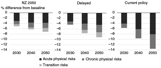
Kalkhul and Wenz estimates have been included in the quantitative assessment of physical risks in the NGFS scenarios. These scenarios also distinguish acute from chronic risk-related impacts. Figure 1.8 shows how GDP would be impacted across scenarios. Short and long-term, acute physical risk emerges as the predominant risk factor. Given its resistance to short-term mitigation efforts, acute physical risk remains consistent across scenarios until 2040, experiencing a significant increase in losses under Current Policies thereafter. Over time, chronic physical risk progressively gains significance, exerting the most substantial adverse impact on GDP within the Current Policies scenario. By 2050, economic losses associated with chronic physical risk will nearly double compared to those projected under the Net Zero 2050 scenario.
Global GDP impact by climate risk source

The climate economic impacts literature typically uses macro-level data (Tol, Reference Tol2009 or Burke et al., Reference Burke, Hsiang and Miguel2015; Dell et al., Reference Dell, Jones and Olken2012). A New Weather Economics literature has recently emerged which assesses the impacts of climate/weather drawing on the aggregation of microeconomic data (e.g., Burke et al., Reference Burke, Hsiang and Miguel2015 or Kolstad and Moore, Reference Kolstad and Moore2019). The microeconomic nature of the data refers both to the sector of activity and to their location, reminding the importance of accounting for the heterogeneity of impacts at industrial and geographical levels when studying the effects of climate change on the economy.
Finally, given the fragmentation of production processes, the impact assessment of climate and weather-related shocks needs to account for their effects along the supply chain. For instance, Forslid and Sanctuary (Reference Forslid and Sanctuary2023) investigate the impact of the severe 2011 Thailand flood on Swedish businesses that relied on imports from Thailand. Results show that output from affected firms decreased by 8 percent in 2012. In total, this led to a reduction of 1.08 billion SEK in imports from Thailand for these firms, resulting in a loss of sales exceeding 29.7 billion SEK. The notable amplification effect underscores the significant repercussions. Despite the relatively swift recovery in Thai production, the effects of the flood persisted, indicating substantial fixed costs associated with establishing supply network connections.
1.4 Conclusion
The exploration of climate change and its economic impacts reveals a multifaceted challenge that demands both immediate attention and long-term strategic thinking. The interconnectedness of environmental, economic, and social systems demonstrates how shifts in climate can profoundly influence economic stability and growth. One key lesson is the critical importance of understanding the scientific underpinnings of climate change, including the roles of the greenhouse effect and human activities, as these are foundational to crafting effective policy responses.
Another significant insight is the potential for irreversible changes and tipping points, which highlights the urgency of timely action. The economic implications of climate change extend far beyond immediate physical risks, impacting everything from asset valuations to national economies. The rising frequency and costs associated with climate-related disasters underscore the importance of preparedness and resilience.
The use of scenario analysis has emerged as a vital tool in climate economics and finance, helping stakeholders anticipate a range of possible futures and the associated economic impacts. This approach facilitates better decision-making and planning by providing a clearer understanding of potential risks and uncertainties.
Overall, the intersection of climate change and economic activity presents both a challenge and an opportunity. The lessons learned emphasize the necessity of integrating climate considerations into economic and financial systems, fostering resilience, and promoting sustainable development.