


1. Introduction
Consider a sequence of independent and identically distributed (i.i.d.) random variables $X_1, \ldots ,X_n$
, each sampled from a population characterized by a risk parameter
$X_1, \ldots ,X_n$
, each sampled from a population characterized by a risk parameter $\theta$
. The Bühlmann credibility, denoted as
$\theta$
. The Bühlmann credibility, denoted as $P^{B.C.}$
, for estimating
$P^{B.C.}$
, for estimating $E(X_{n+1} | X_1, X_2, \ldots , X_n)$
is expressed as a convex combination of the collective premium,
$E(X_{n+1} | X_1, X_2, \ldots , X_n)$
is expressed as a convex combination of the collective premium, $\bar {X}$
and the individual premium
$\bar {X}$
and the individual premium $\mu _0$
, that is,
$\mu _0$
, that is, $P^{B.C.} = \zeta \bar {X} + (1 - \zeta ) \mu _0$
, where the credibility factor
$P^{B.C.} = \zeta \bar {X} + (1 - \zeta ) \mu _0$
, where the credibility factor $\zeta$
is defined as
$\zeta$
is defined as $\zeta = \frac {n}{n + \sigma ^2/\tau ^2}$
, with
$\zeta = \frac {n}{n + \sigma ^2/\tau ^2}$
, with $\sigma ^2 = E\left [Var(X_1|\theta )\right ]$
and
$\sigma ^2 = E\left [Var(X_1|\theta )\right ]$
and $\tau ^2 = Var\left [E(X_1|\theta )\right ]$
.
$\tau ^2 = Var\left [E(X_1|\theta )\right ]$
.
When significant heterogeneity is present within the population, the ratio $\sigma ^2/\tau ^2$
tends toward infinity, causing the credibility factor
$\sigma ^2/\tau ^2$
tends toward infinity, causing the credibility factor $\zeta$
to approach zero. The fundamental task in risk rating is the determination of the so-called pure risk premium
$\zeta$
to approach zero. The fundamental task in risk rating is the determination of the so-called pure risk premium $E[X_i]$
. Such that the pure, or collective, premium is the mean of the hypothetical means. This is the premium we would use if we knew nothing about the individual. It does not depend on the individual’s risk parameter,
$E[X_i]$
. Such that the pure, or collective, premium is the mean of the hypothetical means. This is the premium we would use if we knew nothing about the individual. It does not depend on the individual’s risk parameter, $\theta$
, nor does it utilize
$\theta$
, nor does it utilize $\textbf{X}=\textbf{x}$
, the data collected from the individual. Because
$\textbf{X}=\textbf{x}$
, the data collected from the individual. Because $\theta$
is unknown, the best we can do is leverage the available data, which suggest the use of the Bayesian premium (the mean of the predictive distribution)
$\theta$
is unknown, the best we can do is leverage the available data, which suggest the use of the Bayesian premium (the mean of the predictive distribution) $E(X_{n+1} | X_1, X_2, \ldots , X_n)$
; see Bühlmann and Gisler (2005) and Kass et al. (2008) for more details. Various authors have addressed this issue and proposed potential solutions. For example, Diao and Weng (Reference Diao and Weng2019) introduced the Regression Tree Credibility (RTC) model, while Jahanbani et al. (2024) proposed the Logistic Regression Credibility (LRC) model.
$E(X_{n+1} | X_1, X_2, \ldots , X_n)$
; see Bühlmann and Gisler (2005) and Kass et al. (2008) for more details. Various authors have addressed this issue and proposed potential solutions. For example, Diao and Weng (Reference Diao and Weng2019) introduced the Regression Tree Credibility (RTC) model, while Jahanbani et al. (2024) proposed the Logistic Regression Credibility (LRC) model.
The roots of credibility theory trace back to the seminal works of Mowbray (Reference Mowbray1914) and Whitney (Reference Whitney1918), who proposed a convex combination of collective and individual premiums as the optimal insurance contract premium. Bailey (Reference Bailey1950) formalized this concept, known as the exact credibility premium, within the framework of parametric Bayesian statistics. Building upon this foundation, Bühlmann (1967) and Bühlmann and Straub (1970) expanded the notion of the exact credibility premium to a model-based approach, which significantly contributed to the widespread adoption of credibility theory across various actuarial domains.
There are two distinct approaches to credibility theory: European and American; see Norberg (Reference Norberg1979) for more details. The European approach, often termed Bayesian credibility theory, prioritizes the integration of prior knowledge into the estimation process. It employs Bayesian statistics to incorporate prior beliefs about an insured individual’s risk profile into the prediction of future claims experience. Conversely, the American approach, known for its focus on the credibility premium, relies heavily on past claims data to forecast future losses. Utilizing statistical methods such as the Bühlmann credibility formula, it calculates a credibility factor based on historical data, thereby adjusting the individual’s premium accordingly. Although both approaches aim to enhance risk assessment and premium determination in insurance, they differ in their reliance on prior knowledge and historical data, reflecting distinct methodologies within actuarial practice.
For an in-depth exploration of the evolution and methodologies within credibility theory, Bühlmann and Gisler (2005) and Payandeh Najafabadi (Reference Payandeh Najafabadi2010) provide comprehensive discussions. While classical credibility theory offers a straightforward yet somewhat rigid approach to predictive distribution, for example, Hong and Martin’s research (Reference Hong and Martin2017, Reference Hong and Martin2018) introduced flexible Dirichlet process mixture models for predicting insurance claims and analyzing loss data. Their work demonstrated the effectiveness and adaptability of Bayesian nonparametric frameworks compared to traditional parametric methods. Their research delved into the theoretical underpinnings and benefits of this approach, comparing it with classical credibility theory. Cheung et al. (Reference Cheung, Yam and Zhang2022) and Yong et al. (Reference Yong, Zeng and Zhang2024) offered innovative credibility-based approaches to address challenges in risk estimation and decision-making, integrating concepts from Bayesian hierarchical modeling, prospect theory, and variance premium principle to enhance the accuracy and practicality of actuarial processes. More recently, Gómez-Déniz and Vázquez-Polo (Reference Gómez-Déniz and Vázquez-Polo2022) presented a method for deriving exact credibility reference Bayesian premiums based on prior distributions constructed from available data and a generated model, offering a practical solution when prior information is insufficient for premium determination in credibility theory.
Further advancements in Bayesian credibility theory have focused on the selection of prior distributions, as investigated by Hong and Martin (Reference Hong and Martin2022), highlighting the importance of precise prior specification in Bayesian credibility modeling. The Bayesian credibility mean under mixture distributions has garnered attention from several researchers, including Lau et al. (2006), Cai et al. (Reference Cai, Wen, Wu and Zhou2015), Hong and Martin (Reference Hong and Martin2017, Reference Hong and Martin2018), Zhang et al. (Reference Zhang, Qiu and Wu2018), Payandeh Najafabdi and Sakizadeh (Reference Payandeh Najafabadi and Sakizadeh2019, Reference Payandeh Najafabadi and SakiZadeh2024), Li et al. (2021), and others. However, many of these approaches rely on approximations. For example:
-
(1) Payandeh Najafabadi and Sakizadeh (Reference Payandeh Najafabadi and Sakizadeh2019) employed a mixture distribution to approximate the complex posterior distribution, subsequently deriving an approximation for the Bayesian credibility means. Unfortunately, their approximation error increases with the number of past experiences.
-
(2) Following Lo (1984) and Lau et al. (2006) reformulated the predictive distribution of $X_{n+1}$
given past claim experiences
$X_1, X_2, \ldots , X_n$
as a finite sum over all possible partitions of the past claim experiences. They then utilized the credibility premium, a convex combination of the collective premium (prior mean) and the sample average of past claim experiences, to derive the Bayesian credibility mean. Notably, within the exponential family of distributions, such a credibility premium coincides with the Bayesian credibility mean, as detailed by Payandeh Najafabadi (Reference Payandeh Najafabadi2010) and Payandeh Najafabadi et al. (Reference Payandeh Najafabadi, Hatami and Omidi Najafabadi2012).
$X_{n+1}$
given past claim experiences
$X_1, X_2, \ldots , X_n$
as a finite sum over all possible partitions of the past claim experiences. They then utilized the credibility premium, a convex combination of the collective premium (prior mean) and the sample average of past claim experiences, to derive the Bayesian credibility mean. Notably, within the exponential family of distributions, such a credibility premium coincides with the Bayesian credibility mean, as detailed by Payandeh Najafabadi (Reference Payandeh Najafabadi2010) and Payandeh Najafabadi et al. (Reference Payandeh Najafabadi, Hatami and Omidi Najafabadi2012).


On the contrary, the American credibility (for the sake of convince, just say credibility) theory holds a foundational position within actuarial science, recognized as a cornerstone of insurance experience rating (Hickman & Heacox, Reference Hickman and Heacox1999) and tracing its origins back to Whitney (Reference Whitney1918). This theory conceptualizes the net premium of individual risk, denoted as $\mu (\Theta )$
, as a function of a random element
$\mu (\Theta )$
, as a function of a random element $\Theta$
, representing the unobservable characteristics of the individual risk. The (credibility) premium is then calculated as a linear combination of the average rate of individual claims experience and the collective net premium. Credibility theory has evolved into two main streams: limited fluctuation credibility theory and greatest accuracy credibility theory. The former prioritizes stability, aiming to incorporate individual claims experience while maintaining premium stability. Conversely, the latter, widely employed in modern applications, focuses on achieving the minimum mean squared prediction error by utilizing the best linear unbiased estimator to approximate individual net premiums. This approach integrates both individual and collective claims experience to optimize prediction accuracy.
$\Theta$
, representing the unobservable characteristics of the individual risk. The (credibility) premium is then calculated as a linear combination of the average rate of individual claims experience and the collective net premium. Credibility theory has evolved into two main streams: limited fluctuation credibility theory and greatest accuracy credibility theory. The former prioritizes stability, aiming to incorporate individual claims experience while maintaining premium stability. Conversely, the latter, widely employed in modern applications, focuses on achieving the minimum mean squared prediction error by utilizing the best linear unbiased estimator to approximate individual net premiums. This approach integrates both individual and collective claims experience to optimize prediction accuracy.
This article proceeds under the assumption that through the use of an appropriate classification method, a random sample of observations $\textbf{X} = (X_1, X_2, \ldots , X_n)$
can be effectively categorized into
$\textbf{X} = (X_1, X_2, \ldots , X_n)$
can be effectively categorized into $k$
distinct homogeneous subpopulations
$k$
distinct homogeneous subpopulations $\textbf{X}_l = (X_1, X_2, \ldots , X_{n_l})$
for
$\textbf{X}_l = (X_1, X_2, \ldots , X_{n_l})$
for $l=1,2,\ldots,k$
(
$l=1,2,\ldots,k$
( $n_l$
is the number of observations that fall into class
$n_l$
is the number of observations that fall into class $l$
). It then introduces the expression:
$l$
). It then introduces the expression:
 \begin{equation*}P^{{\rm MCF}} = \sum _{l=1}^{k} \omega _l P^{{\rm Cred}}_{l}=\sum _{l=1}^{k}\omega _l\{\alpha _l{\bar X}_l+(1-\alpha _l)\mu _l\},\end{equation*}
where $\omega _l$
are premium mixture weights obtained based on a statistical technique, such as the logistic regression, such that
$\omega _l$
are premium mixture weights obtained based on a statistical technique, such as the logistic regression, such that $\sum _{l=1}^{k}\omega _l=1,$ $\alpha _l$
credibility weight for class
$\alpha _l$
credibility weight for class $l$
as
$l$
as $\alpha _l= n_l / (n_l + \sigma ^2_l / \tau ^2_l),$ $\mu _l,$
is collective premium of class
$\mu _l,$
is collective premium of class $l$
and
$l$
and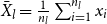 ${\bar X}_l=\frac {1}{n_l} \sum _{i=1}^{n_l} x_i$
for
${\bar X}_l=\frac {1}{n_l} \sum _{i=1}^{n_l} x_i$
for $l=1,2,\ldots , k$
.
$l=1,2,\ldots , k$
.
The rest of this article unfolds as follows: Section 2 elucidates our model assumptions, provides an overview of the Bayesian credibility model, explores the advantages of data space partitioning, and outlines a general credibility model based on partitioning. Section 3 delineates the process of formulating a Mixture Credibility Formula (MCF) and explains the procedure for premium prediction calculations. Section 4 applies our MCF-based prediction model to real-world Medicare data. Finally, Section 5 summarizes the results of the article.
2. Preliminaries and model assumptions
In classical insurance analysis, the treatment of insurance claims typically revolves around modeling them as random variables, denoted as $X$
, with corresponding density functions represented by
$X$
, with corresponding density functions represented by $f(x|\theta )$
. Here,
$f(x|\theta )$
. Here, $\theta$
signifies a fixed parameter associated with the risk, though often obscured by uncertainty. However, the Bayesian approach to risk analysis introduces a fundamental shift in perspective:
$\theta$
signifies a fixed parameter associated with the risk, though often obscured by uncertainty. However, the Bayesian approach to risk analysis introduces a fundamental shift in perspective: $\theta$
is no longer regarded as a fixed value but rather as a random variable itself. This paradigmatic change necessitates the adoption of prior distributions for
$\theta$
is no longer regarded as a fixed value but rather as a random variable itself. This paradigmatic change necessitates the adoption of prior distributions for $\Theta$
within heterogeneous insurance portfolios.
$\Theta$
within heterogeneous insurance portfolios.
The Bayesian framework offers considerable advantages to actuaries. First, it liberates them from the constraints of specific models, fostering adaptability in tackling a wide array of problems. Once adept at analyzing one scenario, actuaries find themselves equipped to handle analogous, albeit more intricate, situations with minimal additional complexity. This inherent flexibility is invaluable in navigating the dynamic landscape of insurance and risk management.
Second, the Bayesian approach simplifies the process of obtaining estimates. Notably, it provides a seamless transition from obtaining point estimates to deriving interval estimates. Also, the key point in the Bayesian approach is it allows actuaries to assess the uncertainty of their inference in terms of probabilities. This characteristic is particularly pertinent in contemporary actuarial practice, where stakeholders increasingly demand not only precise estimates but also insights into the uncertainty surrounding them.
By embracing the Bayesian framework, actuaries can navigate the complexities of risk analysis with greater confidence and efficiency. It empowers them to provide robust evidence regarding the quality and reliability of their estimates, thereby enhancing decision-making processes within the insurance and financial industries. As the landscape of risk management continues to evolve, the Bayesian approach stands as a beacon of innovation and adaptability in the pursuit of informed decision-making and risk mitigation strategies.
Consider a scenario where $X_1, X_2, \ldots , X_n$
represent a vector of insurance claims, while
$X_1, X_2, \ldots , X_n$
represent a vector of insurance claims, while $Z_i = (Z_{i1}, Z_{i2}, \ldots , Z_{im})$
denotes the covariate vector associated with individual risk
$Z_i = (Z_{i1}, Z_{i2}, \ldots , Z_{im})$
denotes the covariate vector associated with individual risk $\theta _i$
, for
$\theta _i$
, for $i = 1, 2, \ldots , n$
. Each individual risk is characterized by a unique risk profile, encapsulated by a scalar
$i = 1, 2, \ldots , n$
. Each individual risk is characterized by a unique risk profile, encapsulated by a scalar $\theta _i$
. Importantly,
$\theta _i$
. Importantly, $\theta _i$
is not a fixed parameter but rather a realization of a random element denoted as
$\theta _i$
is not a fixed parameter but rather a realization of a random element denoted as $\Theta _i$
, reflecting the inherent uncertainty associated with each individual’s risk profile.
$\Theta _i$
, reflecting the inherent uncertainty associated with each individual’s risk profile.
Continuing from the above, let us use the following to elaborate on the division of observations into homogeneous subpopulations:
Model Assumption 1.
Assume that aside nonhomogeneous random sample $X_1, X_2, \ldots ,X_n,$
there is some extra information, restated under covariates
$X_1, X_2, \ldots ,X_n,$
there is some extra information, restated under covariates $Z_1,Z_2,\ldots,Z_m$
where using such extra information, one may partition such random sample into
$Z_1,Z_2,\ldots,Z_m$
where using such extra information, one may partition such random sample into $k$
homogeneous subpopulations,
$k$
homogeneous subpopulations, $\mathcal{I}_1,\mathcal{I}_2,\ldots,\mathcal{I}_k$
. Moreover, suppose that the risk parameter for such subpopulations can be restated as
$\mathcal{I}_1,\mathcal{I}_2,\ldots,\mathcal{I}_k$
. Moreover, suppose that the risk parameter for such subpopulations can be restated as $\Theta _1,\Theta _2,\ldots,\Theta _k$
where
$\Theta _1,\Theta _2,\ldots,\Theta _k$
where $\mu _l=E_{\Theta _l}(E(X_i^{(l)}|\Theta _l)),$ $\sigma _l^2=E_{\Theta _l}\left [Var(X_i^{(l)}|\Theta _l)\right ],$ $\tau _l^2=Var_{\Theta _l}\left [E(X_i^{(l)}|\Theta _l)\right ],$
and
$\tau _l^2=Var_{\Theta _l}\left [E(X_i^{(l)}|\Theta _l)\right ],$
and $n_l=\#\mathcal{I}_l$
(the notation
$n_l=\#\mathcal{I}_l$
(the notation $\#\mathcal{I}_l$
represents the number of observations or data points in the subpopulation identified as
$\#\mathcal{I}_l$
represents the number of observations or data points in the subpopulation identified as $\mathcal{I}_l$
).
$\mathcal{I}_l$
).
Note 1. Under the Model Assumption 1 , one should note that:
-
(1) The credibility formula for the
$l{{\rm th}}$
subpopulation would be
$P^{{\rm Credibility}}_l=\alpha _l\bar {X}_l+(1-\alpha _l) \mu _l$
, where
$\alpha _l = n_l/(n_l + \sigma _l^2/\tau _l^2).$
However, without the above partitioning that the Model Assumption (
1
) recommended, the credibility formula for the entire of population is
$P^{{\rm Credibility}}_{{\rm Total}}=\alpha \bar {X}+(1-\alpha ) \mu ,$
where
$\alpha = n/(n+ \sigma ^2/\tau ^2).$
-
(2) Under the square error loss function, the risk function for the above estimators, respectively, is
\begin{eqnarray*} R^{{\rm Credibility}}_{{\rm Total}}\Big(P^{{\rm Credibility}}_{{\rm Total}}\Big)&=&E\bigg [\Big (P^{{\rm Credibility}}_{{\rm Total}}-\mu (\Theta )\bigg )^2\Big ] = \frac {1}{\frac {n}{\sigma ^2}+\frac {1}{\tau ^2}}\\ R_l^{{\rm Credibility}}\Big(P^{{\rm Credibility}}_{l}\Big)&=&E\bigg [\Big (P^{{\rm Credibility}}_l-\mu (\Theta _l)\Big )^2\bigg ] = \frac {1}{\frac {n_l}{\sigma ^2_l}+\frac {1}{\tau ^2_l}}, \end{eqnarray*}






where $l=1,2,\ldots,k.$
Classification of the nonhomogeneous random sample $X_1, X_2, \ldots ,X_n,$
into
$X_1, X_2, \ldots ,X_n,$
into $k$
homogeneous subpopulation, suggested by Model Assumption 1, plays a crucial role in insurance pricing, leveraging observable characteristics to group insured individuals with similar expected claims. This classification enables the development of premium rating systems, which express a priori information about new policyholders or insured individuals lacking claims experience. However, a priori classification schemes may not capture all relevant factors for premium rating, as some factors are unmeasurable or unobservable.
$k$
homogeneous subpopulation, suggested by Model Assumption 1, plays a crucial role in insurance pricing, leveraging observable characteristics to group insured individuals with similar expected claims. This classification enables the development of premium rating systems, which express a priori information about new policyholders or insured individuals lacking claims experience. However, a priori classification schemes may not capture all relevant factors for premium rating, as some factors are unmeasurable or unobservable.
Classification of the nonhomogeneous random sample $X_1,X_2,\ldots ,X_n$
into
$X_1,X_2,\ldots ,X_n$
into $k$
homogeneous subpopulations, as suggested by Model Assumption 1, plays a crucial role in insurance pricing. This process leverages observable characteristics to group insured individuals with similar expected claims. Such classification enables the development of premium rating systems, which provide initial information about new policyholders or insured individuals lacking claims experience. However, these a priori classification schemes might overlook certain relevant factors in premium rating, as some factors are unmeasurable or unobservable.
$k$
homogeneous subpopulations, as suggested by Model Assumption 1, plays a crucial role in insurance pricing. This process leverages observable characteristics to group insured individuals with similar expected claims. Such classification enables the development of premium rating systems, which provide initial information about new policyholders or insured individuals lacking claims experience. However, these a priori classification schemes might overlook certain relevant factors in premium rating, as some factors are unmeasurable or unobservable.
To address these limitations, a posteriori classification, also known as experience rating, becomes essential. This system re-rates risks by incorporating claims experience into the rating process, resulting in a more equitable and rational price discrimination scheme. By integrating actual claims data, insurers can refine their pricing strategies, better align premiums with individual risk profiles, and promote fairness in insurance pricing.
Diao and Weng (Reference Diao and Weng2019) introduced the RTC model, which employs statistical techniques like regression trees to partition the measurable space $X$
into smaller regions where simple models provide accurate fits. In the subsequent step, for each region, they apply the Bühlmann-Straub credibility premium formula to predict the credibility premium. Specifically, given observed data
$X$
into smaller regions where simple models provide accurate fits. In the subsequent step, for each region, they apply the Bühlmann-Straub credibility premium formula to predict the credibility premium. Specifically, given observed data $X_i$
and associated information
$X_i$
and associated information $Z_{i,1}, \ldots , Z_{i,m}$
for
$Z_{i,1}, \ldots , Z_{i,m}$
for $i=1,\ldots,n$
, a statistical model such as a regression tree determines the probability that the claim experience
$i=1,\ldots,n$
, a statistical model such as a regression tree determines the probability that the claim experience $X_1,X_2,\ldots,X_{n}$
arises from Population
$X_1,X_2,\ldots,X_{n}$
arises from Population $l$
. If this probability exceeds
$l$
. If this probability exceeds $0.5$
, the credibility premium is predicted using the model developed for Population 1; otherwise, the model developed for Population 2 is used. As the RTC method employs the Bühlmann-Straub credibility premium formula, its credibility premium is given by
$0.5$
, the credibility premium is predicted using the model developed for Population 1; otherwise, the model developed for Population 2 is used. As the RTC method employs the Bühlmann-Straub credibility premium formula, its credibility premium is given by $P^{{\rm RTC}}_l = \alpha _l \bar {X}_l + (1-\alpha _l) \mu _l$
when Population
$P^{{\rm RTC}}_l = \alpha _l \bar {X}_l + (1-\alpha _l) \mu _l$
when Population $l=1,2,\ldots,k$
is chosen. However, without any classification, the credibility premium is
$l=1,2,\ldots,k$
is chosen. However, without any classification, the credibility premium is $P^{{\rm Credibility}}_{{\rm Total}}=\alpha \bar {X}+(1-\alpha ) \mu$
, where
$P^{{\rm Credibility}}_{{\rm Total}}=\alpha \bar {X}+(1-\alpha ) \mu$
, where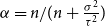 $\alpha ={n}/{(n + \frac {\sigma ^2}{\tau ^2})}$
.
$\alpha ={n}/{(n + \frac {\sigma ^2}{\tau ^2})}$
.
The following provides a more general version of Diao and Weng (Reference Diao and Weng2019)’s finding for the RTC model under the square error loss function:
Theorem 1. Under the Model Assumption 1 and the square error loss function:
-
(1) The risk function for the Regression Tree Credibility, say,
$\underset {\sim }{R}^{{\rm RTC}}(\cdots )$
, and the Total Credibility, say,
$R^{{\rm Credibility}}_{{\rm Total}}(\!\cdot\!),$
respectively, are given by
where
\begin{align*} \underset {\sim }{R}^{{\rm RTC}}\Big(P^{{\rm RTC}}_1,P^{{\rm RTC}}_2,\ldots,P^{{\rm RTC}}_k\Big)&= \sum _{l=1}^{k}\omega _l\bigg [\alpha _l^2 \frac {\sigma _l^2}{n} + (1-\alpha _l)^2 \tau _l^2\bigg ]=\sum _{l=1}^{k}\omega _l \bigg [\frac {1}{\frac {n_l}{\sigma _l^2} + \frac {1}{\tau _l^2}}\bigg ]\\ R_{{\rm Total}}^{{\rm Credibility}}\Big(P^{{\rm Credibility}}_{{\rm Total}}\Big)&=\alpha ^2 \frac {\sigma ^2}{n} + (1-\alpha )^2 \tau ^2 = \frac {1}{\frac {n}{\sigma ^2} + \frac {1}{\tau ^2}} \end{align*}
$\sigma _l^2$
represents the variance of the subpopulation
$l$
,
$\tau _l^2$
denotes the variance of the subpopulation mean, and
$n_l$
represents the number of observations in subpopulation
$l$
.
-
(2) Under the extra assumptions
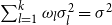
$\sum _{l=1}^{k}\omega _l\sigma _l^2=\sigma ^2$
and
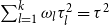
$\sum _{l=1}^{k}\omega _l\tau _l^2=\tau ^2$
, the Regression Tree Credibility premium
$P^{{\rm RTC}}$
, dominates the Total Credibility
$P^{{\rm Credibility}}_{{\rm Total}}$
, that is,
$\underset {\sim }{R}^{{\rm RTC}}(\cdots )\leq R_{{\rm Total}}^{{\rm Credibility}}(\!\cdot\!)$
.





Proof.
To drive an induction argumentation, consider the case of $k=2$
. Using the concave function
$k=2$
. Using the concave function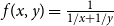 $f(x,y) = \frac {1}{1/{x}+1/{y}}$
, we may conclude that
$f(x,y) = \frac {1}{1/{x}+1/{y}}$
, we may conclude that
 \begin{align*} \underset {\sim }{R}^{{\rm RTC}} \Big(P_1^{{\rm RTC}}, P_2^{{\rm RTC}}\Big)&= \sum _{l=1}^{2}\omega _lf\bigg(\frac {\sigma _l^2}{n},\tau _l^2\bigg)\\ &\leq f\bigg(\omega _1\frac {\sigma _1^2}{n} + \omega _2\frac {\sigma _2^2}{n}, \omega _1 \tau _1^2 + \omega _2 \tau _2^2 \bigg)\\ &=R_{{\rm Total}}^{{\rm Credibility}}(P^{{\rm Credibility}}). \end{align*}
The rest of the proof arrives under an induction argumentation.
Theorem 1 provides key insights into the risk management implications of utilizing the RTC premium within insurance pricing frameworks. By considering the square error loss function, it underscores the significance of balancing within-subpopulation variance $\sigma _l^2$
with between-subpopulation variance
$\sigma _l^2$
with between-subpopulation variance $\tau _l^2$
. This balance is essential for optimizing the mixing proportions
$\tau _l^2$
. This balance is essential for optimizing the mixing proportions $\omega$
to minimize overall risk, highlighting the importance of strategic decision-making in risk assessment and pricing strategies.
$\omega$
to minimize overall risk, highlighting the importance of strategic decision-making in risk assessment and pricing strategies.
Furthermore, the theorem establishes that incorporating subclassifications based on $\omega$
into the MCF premium does not increase the overall risk. In fact, it suggests that the resulting risk is no greater than that associated with
$\omega$
into the MCF premium does not increase the overall risk. In fact, it suggests that the resulting risk is no greater than that associated with $P^{{\rm Bayes}}$
(Bayes premium) without subclassifications. This implies that subclassification strategies improve risk management efficacy without elevating overall risk levels, emphasizing the effectiveness of the RTC premium in refining pricing strategies and enhancing risk assessment accuracy.
$P^{{\rm Bayes}}$
(Bayes premium) without subclassifications. This implies that subclassification strategies improve risk management efficacy without elevating overall risk levels, emphasizing the effectiveness of the RTC premium in refining pricing strategies and enhancing risk assessment accuracy.
Additionally, Theorem 1 elucidates that partitioning a collective of individual risks does not compromise the prediction accuracy of the RTC formula premium, provided that structural parameters of resulting sub-collectives can be accurately computed. While this theoretical foundation supports the use of partitioning-based premium prediction methods, it also acknowledges the inevitability of statistical estimation errors. The challenge lies in balancing the benefits of partitioning against the adverse effects of estimation errors, necessitating a judicious trade-off in decision-making processes.
Model Assumption 2.
Additional to Model Assumption
1
, suppose that for each random variable $X_i$
, for
$X_i$
, for $i=1,2,\ldots,n$
, there exists additional information
$i=1,2,\ldots,n$
, there exists additional information $Z_{i,1}, Z_{i,2}, \ldots , Z_{i,m}$
such that using the following logistic regression, one can evaluate the probability that observation belongs to the
$Z_{i,1}, Z_{i,2}, \ldots , Z_{i,m}$
such that using the following logistic regression, one can evaluate the probability that observation belongs to the $l{{\rm th}}$
subpopulation, that is,
$l{{\rm th}}$
subpopulation, that is,
 \begin{align} \omega _l = P(X_i \in PoP_l|z_{i,1}, z_{i,2}, \ldots , z_{i,m}) = \frac {1} {1+\exp {\{-\beta _{0} - \sum _{j=1}^{m}\beta _{l}z_{j,l}}\}}, \end{align}
for $l=1,2,\ldots,k.$
Moreover, suppose that the claim experience
$l=1,2,\ldots,k.$
Moreover, suppose that the claim experience $X_1,X_2,\ldots,X_n$
, given parameter vector
$X_1,X_2,\ldots,X_n$
, given parameter vector $\boldsymbol{\Psi }=(\theta _1,\theta _2,\ldots,\theta _k)^\prime$
, follows a
$\boldsymbol{\Psi }=(\theta _1,\theta _2,\ldots,\theta _k)^\prime$
, follows a $k$
-component normal mixture distribution
$k$
-component normal mixture distribution $\sum _{l=1}^{k}\omega _l N(\theta _l,\sigma _l^2)$
, where
$\sum _{l=1}^{k}\omega _l N(\theta _l,\sigma _l^2)$
, where $\sigma _l^2$
are given, and for
$\sigma _l^2$
are given, and for $l=1,2,\ldots,k$
,
$l=1,2,\ldots,k$
, $\Theta _l$
has a conjugate prior distribution
$\Theta _l$
has a conjugate prior distribution $N(\mu _l,\tau _l^2)$
.
$N(\mu _l,\tau _l^2)$
.
Under Model Assumption 2, Jahanbani et al. (2024) introduced the LRC premium as $\sum _{l=1}^{k}\omega _l[\xi _1\bar {X}_l+(1-\xi _l)\mu _l] .$
They also showed that, under the squared error loss function, its corresponding risk function is:
$\sum _{l=1}^{k}\omega _l[\xi _1\bar {X}_l+(1-\xi _l)\mu _l] .$
They also showed that, under the squared error loss function, its corresponding risk function is:
 \begin{eqnarray*} R^{{\rm LRC}}(P^{{\rm LRC}}) &=&\sum _{l=1}^{k}\omega _l^2 \bigg [ \xi _l^2 \frac {\sigma _l^2}{n} + (1-\xi _l)^2 \tau _l^2 \bigg ], \end{eqnarray*}
where $\xi _l=\sum _{i=0}^{n} \omega ^i_l (1-\omega _l)^{n-i}\binom {n}{i}\frac {i\tau _l^2}{i\tau _l^2 + \sigma _l^2}.$
Also, it has been shown that in the case of $k=2,$
the LRC premium dominates. Jahanbani et al. (2024) demonstrated that under certain conditions, the risk function of LRC dominates the RTC premium whenever
$k=2,$
the LRC premium dominates. Jahanbani et al. (2024) demonstrated that under certain conditions, the risk function of LRC dominates the RTC premium whenever $\omega$
is around
$\omega$
is around $0.5$
. Additionally, see Jahanbani et al. (2022) for practical applications of the RTC model.
$0.5$
. Additionally, see Jahanbani et al. (2022) for practical applications of the RTC model.
3. Mixture credibility formula
This section serves as the main contribution of this article, presenting the introduction of an MCF model. This model integrates the $k$
-means technique into credibility theory, aiming to improve premium prediction accuracy as measured by the risk function under the square error loss function. Through the incorporation of machine learning methods, the MCF model demonstrates enhanced performance compared to traditional approaches in credibility theory.
$k$
-means technique into credibility theory, aiming to improve premium prediction accuracy as measured by the risk function under the square error loss function. Through the incorporation of machine learning methods, the MCF model demonstrates enhanced performance compared to traditional approaches in credibility theory.
Our MCF model offers a versatile approach to leverage covariate information for premium prediction, consisting of three key steps. First, we introduce a $k$
-means-based algorithm to utilize covariate information, effectively partitioning a collective of risks into distinct sub-collectives. This segmentation ensures homogeneity within each sub-collective while promoting heterogeneity across sub-collectives in terms of risk profiles. Second, the credibility premium formula is applied to each sub-collective, enabling precise estimation of premiums tailored to the characteristics of each segment. Lastly, we aggregate these segment-specific credibility premiums to derive the overall insurance premium, employing logistic regression to estimate mixture weights for each class. This comprehensive approach maximizes the utilization of covariate information while enhancing the accuracy and flexibility of premium prediction.
$k$
-means-based algorithm to utilize covariate information, effectively partitioning a collective of risks into distinct sub-collectives. This segmentation ensures homogeneity within each sub-collective while promoting heterogeneity across sub-collectives in terms of risk profiles. Second, the credibility premium formula is applied to each sub-collective, enabling precise estimation of premiums tailored to the characteristics of each segment. Lastly, we aggregate these segment-specific credibility premiums to derive the overall insurance premium, employing logistic regression to estimate mixture weights for each class. This comprehensive approach maximizes the utilization of covariate information while enhancing the accuracy and flexibility of premium prediction.
The following theorem evaluates the risk function for the MCF when the square error loss function is employed.
Theorem 2.
Under Model Assumption
1
, and probabilities of belonging to each class $(\omega _1, \omega _2, \ldots , \omega _k)$
, the total premium is computed as
$(\omega _1, \omega _2, \ldots , \omega _k)$
, the total premium is computed as $P^{{\rm MCF}} = \sum _{l=1}^{k}\omega _l [\alpha _l \bar {X_l} + (1-\alpha _l) \mu _l]$
. Consequently, the total risk function under the square error loss function can be expressed as follows:
$P^{{\rm MCF}} = \sum _{l=1}^{k}\omega _l [\alpha _l \bar {X_l} + (1-\alpha _l) \mu _l]$
. Consequently, the total risk function under the square error loss function can be expressed as follows:
 \begin{eqnarray*} R^{{\rm MCF}}(P^{{\rm MCF}})&=&\sum _{l=1}^{k} \omega _l^2\bigg [\alpha _l^2 \frac {\sigma _l^2}{n_l} + (1-\alpha _l)^2 \tau _l^2\bigg ]. \end{eqnarray*}
Proof. Using the Model Assumption 1, one may write
 \begin{eqnarray*} R^{{\rm MCF}}(P^{{\rm MCF}})&=& E\bigg [(P^{{\rm MCF}}- \mu (\Theta ))^2\bigg ]=E\bigg [\bigg(P^{{\rm MCF}}- \sum _{l=1}^{k}\omega _l\mu (\Theta _l) \bigg)^2\bigg ]\\ &=&E\bigg [\bigg (\sum _{l=1}^{k}\bigg [\omega _l[\alpha _l \bar {X_l} + (1-\alpha _l) \mu _l] - \omega _l\mu (\Theta _l)\bigg ]\bigg )^2\bigg ]\\ &=&E\bigg [\bigg (\sum _{l=1}^{k}\bigg [\omega _l[\alpha _l \bar {X_l} + (1-\alpha _l) \mu _l] - \omega _l\mu (\Theta _l)\pm \omega _l\alpha _l \mu (\Theta _l)\bigg ]\bigg )^2\bigg ]\\ &=&\sum _{l=1}^{k}\omega _l^2\alpha _l^2 E\bigg [\bigg ( \bar {X_l}-\mu (\Theta _l)\bigg )^2\bigg ] + \sum _{l=1}^{k}\omega _l^2(1-\alpha _l)^2 E\bigg [\bigg ( \mu _l-\mu (\Theta _l)\bigg )^2\bigg ] \\ &=& \sum _{l=1}^{k}\omega _l^2\alpha _l^2 \frac {\sigma _l^2}{n_l} + \sum _{l=1}^{k}\omega _l^2(1-\alpha _l)^2 Var\left [\mu (\Theta _l)\right ] \\ &=&\sum _{l=1}^{k} \omega _l^2\bigg [\alpha _l^2 \frac {\sigma _l^2}{n_l} + (1-\alpha _l)^2 \tau _l^2\bigg ]. \end{eqnarray*}
The following theorem demonstrates that the MCF under the square error loss function outperforms the RTC method introduced by Diao and Weng (Reference Diao and Weng2019).
Theorem 3.
Under the Model Assumption
1
, the MCF under the square error loss function outperforms the RTC, that is, $R^{{\rm MCF}}(\!\cdot\!) \leq \underset {\sim }{R}^{{\rm RTC}}(\cdots ).$
Proof.
Using the result of the above two theorems along with the fact that for all $l=1,2,\ldots, k$ $0 \leq \omega _l\leq 1$
, one may have:
$0 \leq \omega _l\leq 1$
, one may have:
 \begin{align*} &R^{{\rm MCF}}(P^{{\rm MCF}}) - \underset {\sim }{R}^{{\rm RTC}}\Big(P_1^{{\rm RTC}},\ldots, P_k^{{\rm RTC}}\Big) \\&\quad = \sum _{l=1}^{k}\omega _l^2\bigg [\alpha _l^2 \frac {\sigma _l^2}{n_l} + (1-\alpha _l)^2 \tau _l^2\bigg ] -\sum _{l=1}^{k} \omega _l\bigg [\alpha _l^2 \frac {\sigma _l^2}{n_l} + (1-\alpha _l)^2 \tau _l^2\bigg ]\\ &\quad = \sum _{l=1}^{k} \bigg [\alpha _l^2 \frac {\sigma _l^2}{n_l} + (1-\alpha _l)^2 \tau _l^2\bigg ]\omega _l(\omega _l-1)\leq 0. \end{align*}
We proceed to compare the LRC model with the MCF. Specifically, we demonstrate, under the assumption of normality, that the MCF dominates the LRC model.
Theorem 4.
Under the Model Assumption
2
, the MCF premium under the square error loss function dominates the LRC, that is, $R^{{\rm MCF}}(\!\cdot\!) \leq R^{{\rm LRC}}(\!\cdot\!).$
Proof.
In the case of $k=2,$
the difference between the risk functions of two premiums can be restated as
$k=2,$
the difference between the risk functions of two premiums can be restated as
 \begin{align*} &R^{{\rm MCF}}(P^{{\rm MCF}}) - R^{{\rm LRC}}(P^{{\rm LRC}})\\&\quad =\sum _{l=1}^{2} \omega _l^2 \bigg [ \alpha _l^2 \frac {\sigma _l^2}{n_l} + (1-\alpha _l)^2 \tau _l^2 \bigg ] - \sum _{l=1}^{2}\omega _l^2\bigg [ \xi _l^2 \frac {\sigma _l^2}{n_l} + (1-\xi _l)^2 \tau _l^2 \bigg ] \\ &\quad=\sum _{l=1}^{2} \omega _l^2\frac {\sigma _l^2}{n_l}\bigg [ \alpha _l^2 -\xi _l^2\bigg ] +\sum _{l=1}^{2} \omega _l^2 \tau _l^2 \bigg [(1-\alpha _l)^2 - (1-\xi _l)^2\bigg ]\\ &\quad =\sum _{l=1}^{2} \omega _l^2\frac {\sigma _l^2}{n_l} \sum _{i=0}^{n} \omega _l^i (1-\omega _l)^{n-i} \binom {n}{i}\bigg [\frac {n_l\tau _l^2}{n_l\tau _l^2 + \sigma _l^2} +\frac {i\tau _l^2}{i\tau _l^2 + \sigma _l^2}\bigg ]\bigg [\frac {n_l\tau _l^2}{n_l\tau _l^2 + \sigma _l^2} -\frac {i\tau _l^2}{i\tau _l^2 + \sigma _l^2}\bigg ]\\ &\qquad +\sum _{l=1}^{2} \omega _l^2 \tau _l^2 \sum _{i=0}^{n} \omega _l^i (1-\omega _l)^{n-i} \binom {n}{i}\bigg [\frac {\sigma _l^2 }{n_l\tau _l^2 + \sigma _l^2} + \frac {\sigma _l^2}{i\tau _l^2+\sigma _l^2}\bigg ]\bigg [\frac {\sigma _l^2}{n_l\tau _l^2 + \sigma _l^2} -\frac {\sigma _l^2}{i\tau _l^2+\sigma _l^2}\bigg ] \\ &\quad =\sum _{l=1}^{2} \omega _l^2\frac {\sigma _l^2 \tau _l^2}{n_l} \sum _{i=0}^{n} \omega _l^i (1-\omega _l)^{n-i} \binom {n}{i}\tau _l^2\bigg [\frac {n_l}{n_l\tau _l^2 + \sigma _l^2} +\frac {i}{i\tau _l^2 + \sigma _l^2}\bigg ]\bigg [\frac {n_l}{n_l\tau _l^2 + \sigma _l^2} -\frac {i}{i\tau _l^2 + \sigma _l^2}\bigg ] \\ &\qquad \!\!+\sum _{l=1}^{2} \omega _l^2\frac {\sigma _l^2 \tau _l^2}{n_l} \sum _{i=0}^{n} \omega _l^i (1-\omega _l)^{n-i} \binom {n}{i} n_l\sigma _l^2\bigg [\frac {1}{n_l\tau _l^2 + \sigma _l^2} + \frac {1}{i\tau _l^2+\sigma _l^2}\bigg ]\bigg [\frac {1}{n_l\tau _l^2 + \sigma _l^2} -\frac {1}{i\tau _l^2+\sigma _l^2}\bigg ] \\ &\quad= \sum _{i=0}^{n} \omega _1^i (1-\omega _1)^{n-i} \binom {n}{i}\omega _1^2\frac {\sigma _1^2 \tau _1^2}{n_1}\bigg [\frac {n_1^2\tau _1^2+n_1\sigma _1^2}{(n_1\tau _1^2+\sigma _1^2)^2} - \frac {i^2 \tau _1^2 +n_1\sigma _1^2}{(i\tau _1^2+\sigma _1^2)^2} \bigg ]\\ &\qquad + \sum _{i=0}^{n} (1-\omega _1)^i (\omega _1)^{n-i} \binom {n}{i}(1-\omega _1)^2\frac {\sigma _2^2 \tau _2^2}{n_2}\bigg [\frac {n_2^2\tau _2^2+n_2\sigma _2^2}{(n_2\tau _2^2+\sigma _2^2)^2} - \frac {i^2 \tau _2^2 +n_2\sigma _2^2}{(i\tau _2^2+\sigma _2^2)^2} \bigg ]\\ &\quad =\sum _{i=0}^{n} \omega _1^i (1-\omega _1)^{n-i} \binom {n}{i} H_{(1,2)}(i), \end{align*}
where
 \begin{eqnarray} \nonumber H_{(1,2)}(i)&=&\omega _1^2\frac {\sigma _1^2 \tau _1^2}{n_1}\bigg [\frac {n_1^2\tau _1^2+n_1\sigma _1^2}{(n_1\tau _1^2+\sigma _1^2)^2} - \frac {i^2 \tau _1^2 +n_1\sigma _1^2}{(i\tau _1^2+\sigma _1^2)^2} \bigg ]\\ && +(1-\omega _1)^2\frac {\sigma _2^2 \tau _2^2}{n_2}\bigg [\frac {n_2^2\tau _2^2+n_2\sigma _2^2}{(n_2\tau _2^2+\sigma _2^2)^2} - \frac {(n-i)^2 \tau _2^2 +n_2\sigma _2^2}{((n-i)\tau _2^2+\sigma _2^2)^2} \bigg ] \end{eqnarray}
which arrives by using the fact that $ \binom {n}{i}= \binom {n}{n-i}.$
Now, without loss of generality, assume that the function $H_{(1,2)}(i)$
is a continuous function with respect to
$H_{(1,2)}(i)$
is a continuous function with respect to $i$
. Therefore, using the first derivative
$i$
. Therefore, using the first derivative
 \begin{eqnarray*} \frac {\partial H_{(1,2)}(i)}{\partial i} = - \omega _1^2 \frac {\sigma _1^2 \tau _1^2}{n_1} \frac {2 \tau _1^2 \sigma _1^2 i}{(i \tau _1^2 + \sigma _1^2)^3} + (1-\omega _1)^2 \frac {\sigma _2^2 \tau _2^2}{n_2} \frac {2 \tau _2^2[(n-i)\sigma _2^2-n_2\sigma _2^2]}{((n-i) \tau _2^2 + \sigma _2^2)^3}, \end{eqnarray*}
one may conclude that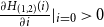 $\frac {\partial H_{(1,2)}(i)}{\partial i}|_{i=0} \gt 0$
and
$\frac {\partial H_{(1,2)}(i)}{\partial i}|_{i=0} \gt 0$
and $\frac {\partial H_{(1,2)}(i)}{\partial i}|_{i=n} \lt 0$
. On the other hand, since
$\frac {\partial H_{(1,2)}(i)}{\partial i}|_{i=n} \lt 0$
. On the other hand, since $\frac {\partial ^2 H_{(1,2)}(i)}{\partial ^2 i} \lt 0,$
one may conclude that
$\frac {\partial ^2 H_{(1,2)}(i)}{\partial ^2 i} \lt 0,$
one may conclude that $H_{(1,2)}(i)$
as a function of
$H_{(1,2)}(i)$
as a function of $i$
is a concave function which attains its maximum at
$i$
is a concave function which attains its maximum at $i=n_1=n-n_2$
in which
$i=n_1=n-n_2$
in which $H_{(1,2)}(i=n_1)= 0.$
Therefore, for the case of
$H_{(1,2)}(i=n_1)= 0.$
Therefore, for the case of $k=2,$
we always have
$k=2,$
we always have $R^{{\rm MCF}}(\!\cdot\!) - R^{{\rm LRC}}(\!\cdot\!)\leq 0.$
Now of the general case of $k\gt 2,$
observe that
$k\gt 2,$
observe that
 \begin{eqnarray*} \omega _k^i(1-\omega _k)^{n-i}&=&(1-\omega _1-\cdots -\omega _{k-1})^i(\omega _1+\cdots +\omega _{k-1})^{n-i}\\ &\leq &\sum _{l=1}^{k-1}\omega _l^i(1-\omega _l)^{n-i}. \end{eqnarray*}
Using the above inequality, the difference between the two risk functions can be bounded above by
 \begin{align*}& R^{{\rm MCF}}(P^{{\rm MCF}}) - R^{{\rm LRC}}(P^{{\rm LRC}})\\&\quad =\sum _{l=1}^{k} \omega _l^2 \bigg [ \alpha _l^2 \frac {\sigma _l^2}{n_l} + (1-\alpha _l)^2 \tau _l^2 \bigg ] - \sum _{l=1}^{k}\omega _l^2\bigg [ \xi _l^2 \frac {\sigma _l^2}{n_l} + (1-\xi _l)^2 \tau _l^2 \bigg ] \\ &\quad =\sum _{l=1}^{k} \omega _l^2\frac {\sigma _l^2}{n_l}\bigg [ \alpha _l^2 -\xi _l^2\bigg ] +\sum _{l=1}^{2} \omega _l^2 \tau _l^2 \bigg [(1-\alpha _l)^2 - (1-\xi _l)^2\bigg ]\\ &\quad =\sum _{l=1}^{k} \omega _l^2\frac {\sigma _l^2}{n_l} \sum _{i=0}^{n} \omega _l^i (1-\omega _l)^{n-i} \binom {n}{i}\bigg [\frac {n_l\tau _l^2}{n_l\tau _l^2 + \sigma _l^2} +\frac {i\tau _l^2}{i\tau _l^2 + \sigma _l^2}\bigg ]\bigg [\frac {n_l\tau _l^2}{n_l\tau _l^2 + \sigma _l^2} -\frac {i\tau _l^2}{i\tau _l^2 + \sigma _l^2}\bigg ]\\ &\qquad+\sum _{l=1}^{k} \omega _l^2 \tau _l^2 \sum _{i=0}^{n} \omega _l^i (1-\omega _l)^{n-i} \binom {n}{i}\bigg [\frac {\sigma _l^2 }{n_l\tau _l^2 + \sigma _l^2} + \frac {\sigma _l^2}{i\tau _l^2+\sigma _l^2}\bigg ]\bigg [\frac {\sigma _l^2}{n_l\tau _l^2 + \sigma _l^2} -\frac {\sigma _l^2}{i\tau _l^2+\sigma _l^2}\bigg ] \\ &\quad=\sum _{l=1}^{k} \omega _l^2\frac {\sigma _l^2 \tau _l^2}{n_l} \sum _{i=0}^{n} \omega _l^i (1-\omega _l)^{n-i} \binom {n}{i}\tau _l^2\bigg [\frac {n_l}{n_l\tau _l^2 + \sigma _l^2} +\frac {i}{i\tau _l^2 + \sigma _l^2}\bigg ]\bigg [\frac {n_l}{n_l\tau _l^2 + \sigma _l^2} -\frac {i}{i\tau _l^2 + \sigma _l^2}\bigg ] \\ &\qquad\!\!+\sum _{l=1}^{k} \omega _l^2\frac {\sigma _l^2 \tau _l^2}{n_l} \sum _{i=0}^{n} \omega _l^i (1-\omega _l)^{n-i} \binom {n}{i} n_l\sigma _l^2\bigg [\frac {1}{n_l\tau _l^2 + \sigma _l^2} + \frac {1}{i\tau _l^2+\sigma _l^2}\bigg ]\bigg [\frac {1}{n_l\tau _l^2 + \sigma _l^2} -\frac {1}{i\tau _l^2+\sigma _l^2}\bigg ] \end{align*}
 \begin{align*}&=\sum _{l=1}^{k}\sum _{i=0}^{n} \omega _l^i (1-\omega _l)^{n-i} \binom {n}{i}\omega _l^2\frac {\sigma _l^2 \tau _l^2}{n_l} \bigg [\frac {n_l^2\tau _l^2+n_l\sigma _l^2}{(n_l\tau _l^2+\sigma _l^2)^2} - \frac {i^2 \tau _l^2 +n_l\sigma _l^2}{(i\tau _l^2+\sigma _l^2)^2} \bigg ]\qquad \qquad \\ &\qquad\leq \sum _{l=1}^{k-1}\sum _{i=0}^{n} \omega _l^i (1-\omega _l)^{n-i} \binom {n}{i} H_{(l,k)}(i), \end{align*}
where $H_{(l,k)}(i)$
is a general version of the
$H_{(l,k)}(i)$
is a general version of the $H_{(1,2)}(i)$
given by Equation (2). The same argument, as we did above for the case
$H_{(1,2)}(i)$
given by Equation (2). The same argument, as we did above for the case $k=2,$
leads to desired result for the general case
$k=2,$
leads to desired result for the general case $k\gt 2$
, that is,
$k\gt 2$
, that is, $ R^{{\rm MCF}}(\!\cdot\!) - R^{{\rm LRC}}(\!\cdot\!) \leq 0$
.
$ R^{{\rm MCF}}(\!\cdot\!) - R^{{\rm LRC}}(\!\cdot\!) \leq 0$
.
4. Application to the real-world data
To illustrate the practical application of the above findings, we now consider a real-world dataset from an Iranian insurance company. This dataset contains demographic information (such as gender, age, etc.) as well as the size of claims for 1,180,255 individuals. Table 1 represents the list of available information in the dataset.
Output of command str(Data)

Figure 1(a) illustrates the box plot of claim size. However, Figure 1(b) illustrates the box plot of claim size after outlier data has been removed from the dataset. We defined an outlier observation as any observation that exceeds the value of 181,727,944 rials (the Iranian currency), and after removing such outlier data, we obtained 1,179,470 individuals.
The box plot of damages’ size before removing outliers (a) and after removing outliers (b).

Figure 2 shows our attempt to fit a statistical distribution to the claim size.
Histogram and density plots of the claim size.

The box plot of damages’ size for different categories.

As one may observe, there is considerable non-homogeneity in the data. Therefore, we decided to derive some subpopulations to homogenize the data.
To get started, we categorized the covariates “Age” into 5 classes and “Province” into 8 classes. The Spearman test validated a significant relationship between age, gender, province, type of insured, and claim size. Moreover, the nonparametric Kruskal–Wallis test revealed a significant difference between groups associated with gender, type of insured, age, and province. Figure 3 shows the box plot of claim size regarding the aforementioned covariates.
Using Figure 3, one may conclude that these covariates can be employed to define some more homogenous subpopulations.
In the next step, using the $k$
-means clustering method, we derived two subpopulations, which classify insured individuals into high-risk and low-risk categories. A bivariate visualization of the two subpopulations is presented in Figure 4. Moreover, Figure 5 illustrates a histogram of claim size for those subpopulations.
$k$
-means clustering method, we derived two subpopulations, which classify insured individuals into high-risk and low-risk categories. A bivariate visualization of the two subpopulations is presented in Figure 4. Moreover, Figure 5 illustrates a histogram of claim size for those subpopulations.
A bivariate visualization of the two subpopulations.

Histogram of claim size for the high-risk and the low-risk classes.

To determine the probability that a given individual belongs to a given subpopulation, we implement the following logistic regression:
 \begin{equation} \omega _1 = P(Y_i\in Pop_1|\textbf{Z}_{\textbf{i}}=\textbf{z}_{\textbf{i}}) =1/\{1+e^{-\beta _{0} -\beta _{1}{z_1}-\beta _{2}{z_2}-\beta _{3}{z_3}-\beta _{4}{z_4}}\}, \end{equation}
where $z_1, z_2, z_3, z_4,$
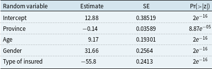
respectively, stand for the re-categorized province, age, gender, and type of insured. Using the least square error method against observed data, we estimated the logistic regression parameters. Table 2 reports such estimated parameters.
$z_1, z_2, z_3, z_4,$
respectively, stand for the re-categorized province, age, gender, and type of insured. Using the least square error method against observed data, we estimated the logistic regression parameters. Table 2 reports such estimated parameters.
Now, as an example, consider a $50$
-year-old single man who lives in a location labeled 6. Moreover, suppose that the logarithms of his
$50$
-year-old single man who lives in a location labeled 6. Moreover, suppose that the logarithms of his $11$
years claim experiences are
$11$
years claim experiences are $16.91,$ $17.68,$ $15.97,$ $19.23,$ $15.63,$ $16.03,$ $14.85,$ $18.41,$ $14.20,$ $16.20$
, and
$16.20$
, and $14.75258.$
Using the logistic regression model (3) against his information, with probability $0.2378$
(
$0.2378$
( $\omega =0.2378$
), he would fall into Class 1. Therefore, the logarithm of the MCF for his next year is
$\omega =0.2378$
), he would fall into Class 1. Therefore, the logarithm of the MCF for his next year is
 \begin{eqnarray*} \log(P^{{\rm MCF}})&=&\omega \left [\left (\frac {n_1}{n_1+\frac {2}{{\hat \tau }_1^2}}\right )\bar {x}_1+\left (1-\frac {n_1}{n_1+\frac {{\hat \sigma }_1^2}{{\hat \tau }_1^2}}\right ){\hat \mu _1}\right ]\\ &=&+ (1-\omega ) \left [\left (\frac {n_2}{n_2+\frac {{\hat \sigma }_2^2}{{\hat \tau }_2^2}}\right )\bar {x}_2+\left (1-\frac {n_2}{n_2+\frac {{\hat \sigma }_2^2}{{\hat \tau }_2^2}}\right ){\hat \mu _2}\right ]\\ &=&0.2378\left [\left (\frac {597253}{597253+\frac {2}{1.48}}\right )17.42+\left (1-\frac {597253}{597253+\frac {2}{1.48}}\right )15\right ]\\ &&+0.7622\left [\left (\frac {582217}{582217+\frac {3}{1.51}}\right )17.83+\left (1-\frac {582217}{582217+\frac {3}{1.51}}\right )20\right ]\\ &=&17.73251. \end{eqnarray*}
5. Conclusion
The insurance industry relies heavily on accurate predictions of future damages and losses. Various methods, including time series analysis, Bayesian methods, and belief theory, are employed for such predictions. Among these, both classical and Bayesian credibility methods offer accurate and robust predictions.
Logistic regression

In this article, under the $k$
-component normal mixture distribution assumption, we introduced the MCF method for insurance premium calculation. This method begins by clustering the insured population into homogeneous subpopulations using data mining techniques, such as
$k$
-component normal mixture distribution assumption, we introduced the MCF method for insurance premium calculation. This method begins by clustering the insured population into homogeneous subpopulations using data mining techniques, such as $k$
-means. Then, the classical credibility premium is evaluated for each subpopulation. The MCF is a convex combination of those classical credibility premiums. For the case of two subpopulations, the convex weight can be determined by using logistic regression. We also compared the performance of the MCF method with the RTC method and the LRC method. Our analysis revealed that the MCF method consistently outperforms those methods in terms of the quadratic loss function. This underscores the effectiveness of the MCF method in refining insurance premium calculations and improving risk assessment strategies.
$k$
-means. Then, the classical credibility premium is evaluated for each subpopulation. The MCF is a convex combination of those classical credibility premiums. For the case of two subpopulations, the convex weight can be determined by using logistic regression. We also compared the performance of the MCF method with the RTC method and the LRC method. Our analysis revealed that the MCF method consistently outperforms those methods in terms of the quadratic loss function. This underscores the effectiveness of the MCF method in refining insurance premium calculations and improving risk assessment strategies.
As mentioned earlier, we derive our findings under the $k$
-component normal mixture distribution assumptions; for a possible extension, one may consider how this restrictive assumption can be removed.
$k$
-component normal mixture distribution assumptions; for a possible extension, one may consider how this restrictive assumption can be removed.
Acknowledgments
The authors thank Dr. Shahram Mansour for his valuable comments and suggestions on an earlier version of this manuscript. Moreover, the authors would like to thank the anonymous reviewers for their constructive comments, which improved the theoretical foundation and presentation of this article.
Data availability statement
The data and code that support the findings of this study are available on request from the corresponding author. The data are not publicly available due to restrictions for the insurance company.
Funding statement
There is no financial support for this article.
Competing interests
The authors declare none.



 Open access

