


1. Introduction
Sea-ice thickness and sea-ice growth rates are important parameters for the study of sea-ice processes and the sea ice–ocean–ice shelf system. The knowledge gaps around sea-ice thickness are identified as one of the key issues that need to be addressed in Southern Ocean observations (Newman and others, Reference Newman2019). Together with sea-ice extent, sea-ice thickness is needed to calculate sea-ice volume as well as defining the mechanical strength of the sea-ice cover (Timco and Weeks, Reference Timco and Weeks2010). However, due to the effects of snow on buoyancy, it is difficult to retrieve sea-ice thickness measurements remotely through observations of freeboard (e.g., Kurtz and Markus, Reference Kurtz and Markus2012). This is further complicated in locations where there is oceanic supercooling forming porous accumulations of crystals under the ice (sub-ice platelet layers (SIPL); e.g., Hoppmann and others, Reference Hoppmann2020) that also influence buoyancy (e.g., Price and others, Reference Price2014).
In situ measurements of sea-ice thickness are traditionally made by drilling holes through the sea ice and measuring the thickness of the ice with a weighted tape. It is still the most common method of measuring sea-ice thickness (see an overview of measurement methods in Haas and Druckenmiller, Reference Haas and Druckenmiller2009). This method is time intensive and relies on access to the sea ice and safe sea-ice conditions for on-ice operations. Repeat measurements in the same location will alter the heat flux at that location through repeated opening and re-freezing of the hole. Since sea ice is not perfectly level, measuring in slightly different locations each time will add a spatial component to the measurements which can be on the order of centimetres (Haas and Druckenmiller, Reference Haas and Druckenmiller2009) to decimetres and especially pronounced in deformed ice, in ice with a SIPL, and in melting ice.
To retrieve sea-ice thickness measurements with a high temporal resolution and minimal disturbance of the sea-ice cover at a single location, the use of Sea Ice Monitoring Stations (SIMS, also commonly referred to as Ice Mass Balance Buoys, IMBs) has become more frequent in both the Arctic and the Antarctic. SIMS can be deployed either on drifting sea-ice floes (e.g., Perovich and Elder, Reference Perovich and Elder2001; Provost and others, Reference Provost2017; Tian and others, Reference Tian2017) or on landfast sea ice (e.g., Trodahl and others, Reference Trodahl2000; Polashenski and others, Reference Polashenski, Perovich, Richter-Menge and Elder2015; Gough and others, Reference Gough2012; Hoppmann and others, Reference Hoppmann2015). Thermistor strings are common components of SIMS and have been used in sea-ice research since the 1980s (e.g., Perovich and others, Reference Perovich, Tucker III and Krishfield1989).
All thermistor strings measure temperature at pre-defined spatial intervals (in general 2–10 cm) vertically throughout the sea ice and, if the ice is not thicker then the probe is long, into the ocean. Some designs also extend upwards to include snow and/or air temperature measurements; a schematic of different SIMS is shown in Figure 1. A generic output from a thermistor string will show coldest temperatures at the ice–snow or ice–atmosphere interface. During ice formation, the sea-ice temperature increases with depth to the ocean freezing point (generally around $-1.8^\circ$ C) at the sea ice–ocean interface. Thermistor strings can therefore provide valuable data on sea-ice growth rates during the winter and spring (e.g., Gough and others, Reference Gough2012).
Schematic of different sea ice monitoring station setups. (a) CRREL Version 1 + 2 design as used at our Arctic site, (b) CRREL Version 3 or Cryosphere Innovation SIMB3 type design, (c) SAMS type design, the thermistor string includes heating elements, (d) VUW/Otago type design as used at our McMurdo Sound station. The TUT buoy is a combination of CRREL version 1 + 2 acoustic sensors and SAMS type thermistor string, though without heating elements.
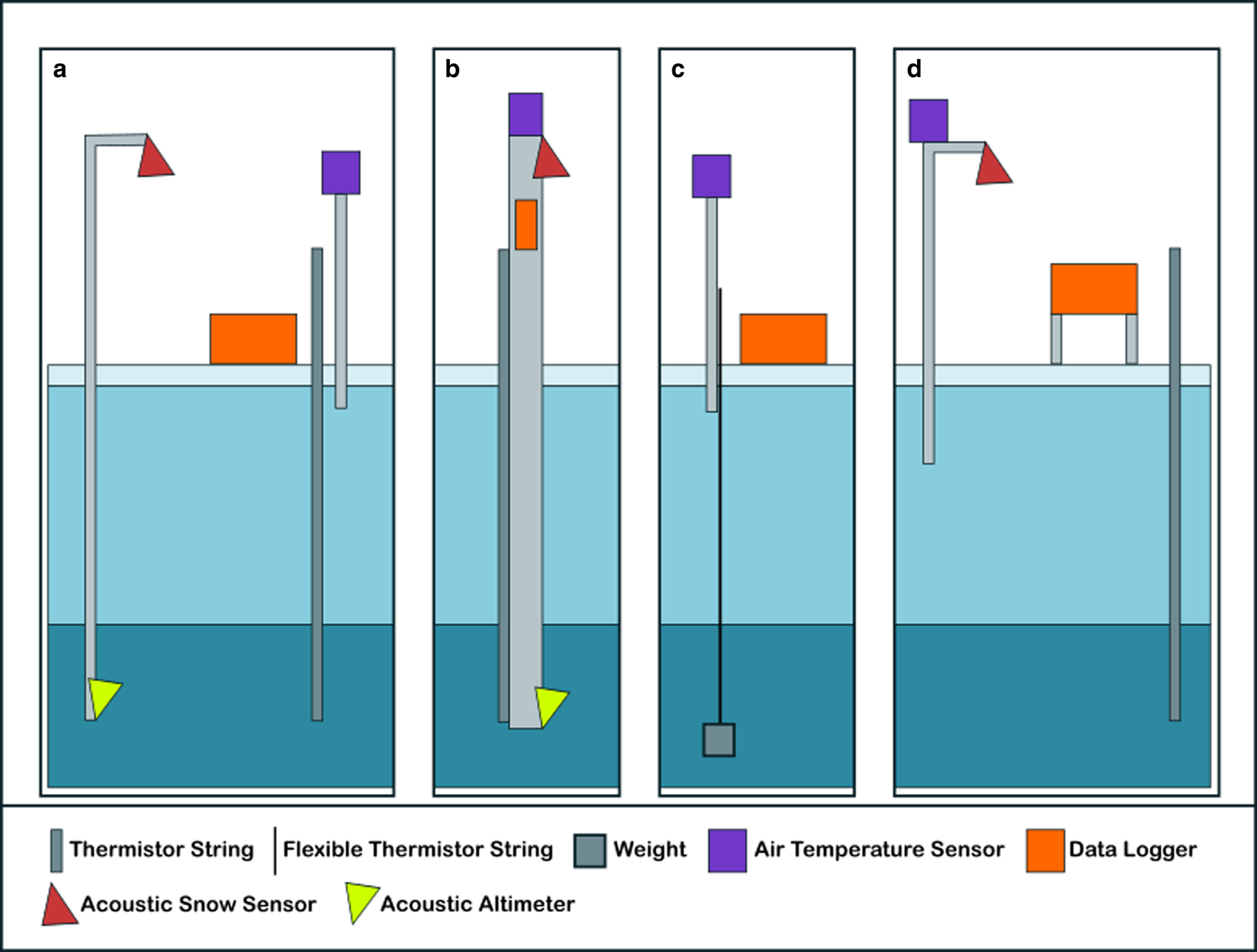
The CRREL buoy designed by the United States Army Cold Regions Research and Engineering Laboratory (CRREL) and Dartmouth College (CRREL website, n.d) includes acoustic sensors for snow height and ice–ocean interface (Fig. 1a; Untersteiner and Thorndike, Reference Untersteiner and Thorndike1984; Richter-Menge and others, Reference Richter-Menge2006). A similar design to the CRREL buoys was used by the Polar Research Institute of China and Taiyuan University of Technology (‘TUT buoy’; Zuo and others, Reference Zuo, Dou and Lei2018). Recent evolutions of the CRREL buoy and a successor design, the Cryosphere Innovation buoy (https://www.cryosphereinnovation.com/simb3) are deployed in a self-righting floating hull to allow measurements into the melt season (Fig. 1b; Polashenski and others, Reference Polashenski, Perovich, Richter-Menge and Elder2015; Planck and others, Reference Planck, Whitlock, Polashenski and Perovich2019). A lower cost alternative to the CRREL buoys, without acoustic sensors, was designed by the Scottish Association for Marine Science (SAMS buoy; Fig. 1c; Jackson and others, Reference Jackson2013). It contains heating elements in the thermistor string allowing a thermal diffusivity proxy to be calculated and is the only thermistor string design capable of also retrieving the SIPL thickness (e.g., Hoppmann and others, Reference Hoppmann2015), the friable layer of crystals which may form in in situ supercooled water (Crocker and Wadhams, Reference Crocker and Wadhams1989; Dayton, Reference Dayton1989; Gough and others, Reference Gough2012; Hoppmann and others, Reference Hoppmann2020). Other designs include thermistors encased in an oil-filled steel tube (developed at Victoria University Wellington, NZ (VUW) and now deployed by the University of Otago, NZ; Fig. 1d; Trodahl and others, Reference Trodahl2000), or protruding from an epoxy-polycarbonate support or PVC rod (Frey and others, Reference Frey2001; Gough and others, Reference Gough2012). The wide variety of SIMS designs and types of data collected leads to different analysis methods, and thus issues comparing data and results from different studies.
Most studies use sea-ice temperature data to determine the ice–ocean interface by examining the vertical gradient of the sea-ice temperature and define the interface as the point where the gradient drops to close to zero in the isothermal ocean boundary layer under the ice (e.g., Perovich and others, Reference Perovich, Tucker III and Krishfield1989, Reference Perovich, Elder and Richter-Menge1997; Perovich and Elder, Reference Perovich and Elder2001; Morison and others, Reference Morison2002), with some authors determining the interface through manual interface detection involving detailed inspection of the data rather than by applying an automated method (e.g., Smith and others, Reference Smith, Langhorne, Frew, Vennell and Haskell2012). Perovich and others (Reference Perovich, Elder and Richter-Menge1997) stated that the ice–ocean interface could be determined within ±1 to ±2 cm from a string with a thermistor spacing of 5–20 cm. However, they also noted that finding the interface from the change in vertical temperature gradient between ice and ocean is not always possible during the melt season, when the temperature of the lower ice column approaches the temperature of the ocean water. In growing sea ice, Gough and others (Reference Gough2012) described an algorithm to automatically retrieve the ice–ocean interface for two thermistor string designs, one with thermistors encased in a steel tube and the other with thermistors protruding from a PVC rod, by examining the vertical temperature gradient at every timestep. We will describe this method in detail in Section 2.5.1.
Previous studies have determined sea-ice thickness from temperature data using various methods: (i) comparison to the ocean freezing-point temperature from CTD casts (Provost and others, Reference Provost2017), which has issues due to the variable freezing point temperature caused by salinity fluctuations from brine and melt pond drainage (e.g., Martin and Kauffman, Reference Martin and Kauffman1974; Notz and others, Reference Notz2003) and advection of different water masses (e.g., Smith and others, Reference Smith2016); (ii) a combination of temperature, vertical temperature gradient and daily amplitude of temperature fluctuations (Zuo and others, Reference Zuo, Dou and Lei2018); (iii) the vertical temperature gradient combined with a thermal diffusivity proxy from heating elements (Hoppmann and others, Reference Hoppmann2015) which is currently the only method to resolve the SIPL; (iv) air, snow, ice and ocean temperature profiles taking into account the heat flux though these media (Liao and others, Reference Liao2018); (v) machine learning on data from SAMS buoys (Hoppmann and others, Reference Hoppmann, Itkin and Tiemann2017; Tiemann and others, Reference Tiemann, Nicolaus, Hoppmann, Huntermann and Haas2018; and Stefanie Arndt and Louisa von Hülsen (formerly Tiemann), pers. comm. by email October 2019). The last group noted that there remained a need to develop a unified processing and data cleaning framework and to further develop and compare the algorithms used. This need for unified methods and long-term sustained observational efforts was also noted by the Antarctic Fast Ice Network (AFIN; Heil and others, Reference Heil, Gerland and Granskog2011) and more recently, by the Southern Ocean Observing System (SOOS; Newman and others, Reference Newman2019). Such a unified method, with an option to calculate error bounds for observations without having repeat observations, would give confidence that potential differences in thickness and growth rate between sites and years are not due to instrument design or analysis. This would then allow more robust large-scale comparisons of data collected by different SIMS designs, such as the datasets available through the International Arctic and Antarctic Buoy programmes (https://iabp.apl.uw.edu/ and https://www.ipab.aq/).
This paper aims to fill this gap by presenting a unified pre-processing routine and comparing the accuracy and precision of different methods of interface detection using datasets from two long-term monitoring stations on landfast sea ice in the Arctic and Antarctic. We will restrict our analysis to ice and ocean temperatures as this is the minimum data recorded by all common SIMS designs. Further, we will restrict ourselves to landfast sea ice during the growth season to avoid biases due to the dynamic nature of pack ice. This allows a more robust comparison of methods. Three methods of automated interface detection will be compared to manual picking of the interface (Section 3) and independent measurements of sea-ice thickness and growth rate (Sections 3.1 and 3.2), where available. We will assess the sensitivity, precision and accuracy of these methods and compare them to values found in the literature (Section 4). Finally, we will make recommendations on future thermistor string design and data processing (Sections 4.3 and 5).
2. Materials and methods
2.1. Study area
2.1.1. McMurdo Sound, Ross Sea, Antarctica
McMurdo Sound is located in the western Ross Sea and is seasonally covered in landfast sea ice. It is not a true sound, as the McMurdo Ice Shelf cavity has a connection to the Ross Ice Shelf cavity in the southeast, allowing water exchange between the cavities (Assmann, Reference Assmann2004; Robinson and others, Reference Robinson, Williams, Barrett and Pyne2010).
The local oceanography is influenced by the outflow of ice shelf water (ISW) from under the McMurdo Ice Shelf (Robinson and others, Reference Robinson, Williams, Barrett and Pyne2010; Robinson, Reference Robinson2012), defined by a potential temperature below the surface freezing point of sea water (potential supercooling; Jacobs and others, Reference Jacobs, Fairbanks and Horibe1985; Jacobs, Reference Jacobs2004). The ISW can become in situ supercooled and contributes to the formation of platelet ice in the sound which influences the fast-ice cover there (e.g., Gow and others, Reference Gow, Ackley, Govoni and Weeks1998; Dempsey and others, Reference Dempsey2010; Langhorne and others, Reference Langhorne2015).
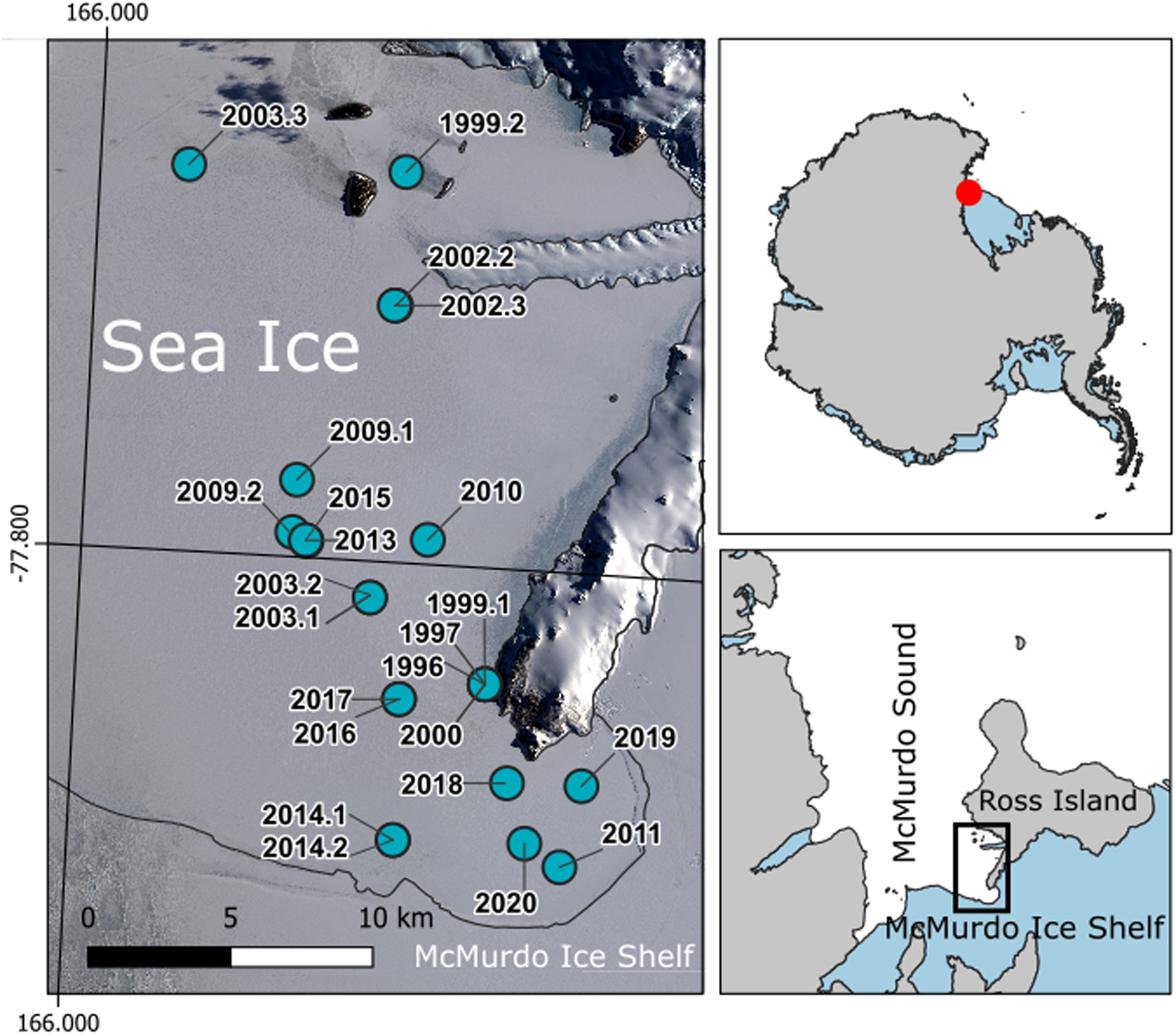
SIMS have been deployed on the landfast ice throughout the eastern sound (see map in Fig. 2) by and for New Zealand Antarctic research teams in most years between 1996 and 2020. The majority of deployments occurred on first-year ice, though some deployments were on multi-year ice (see Table 1).
Map of McMurdo Sound with the location of the SIMS (see Table 1) marked as dots. The location of McMurdo Sound in Antarctica is shown in the top right panel, McMurdo Sound and Ross Island is shown in the bottom right panel with the zoomed in area shown on the left marked by the rectangular box. The background image in the left panel is a pansharpened visible image from Landsat 8 taken on 15 October 2018. Image downloaded from USGS, courtesy of the US Geological Survey. The right hand panels show a map of Antarctica (SCAR Antarctic Digital Database, accessed 2021), with land and grounded ice in grey, and ice shelves and glacier tongues in blue.
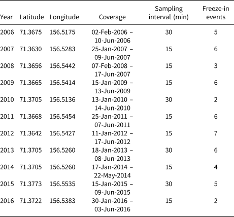
Information on SIMS deployments in McMurdo Sound

Times in NZST, location is approximate for deployments prior to 2003, ice type is (FY) first year ice or (MY) second year ice, design is (SP) steel probe or (EP) epoxy/plastic probe, snow sensor is (y) if a snow sensor was included in the SIMS, freeze-in events is the number of thermistors observed to freeze in during a deployment, notes give information on data quality. For deployment locations also see Figure 2.
The landfast ice in the sound was always over 60 cm thick and had a positive freeboard at the time of SIMS deployment. The positive freeboard remained throughout the growth season and thus snow-ice formation did not contribute to fast-ice growth during that period. In general, snow-ice formation does not play a major role in eastern McMurdo Sound which is confirmed by oxygen isotope and structural analysis of cores (e.g., Smith and others, Reference Smith2001, Reference Smith, Langhorne, Frew, Vennell and Haskell2012, Reference Smith2015; Dempsey and others, Reference Dempsey2010).
2.1.2. Utqiaġvik, Chukchi Sea, Arctic
The Utqiaġvik (formerly Barrow, Alaska) SIMS site, is located in the Chukchi Sea and was maintained by the University of Alaska Fairbanks (UAF). At this location, landfast sea ice generally forms between November and December, with fast ice break-out around June (Druckenmiller and others, Reference Druckenmiller, Eicken, Johnson, Pringle and Williams2009). The SIMS sites have been located on the 1–10 km wide strip of seasonal landfast ice which is held in place by grounded ridges in very shallow water (~5 m; Mahoney and others, Reference Mahoney, Eicken and Shapiro2007) seaward of the Point Barrow spit (Druckenmiller and others, Reference Druckenmiller, Eicken, Johnson, Pringle and Williams2009). The locations of the SIMS can be seen in Figure 3, with the location of Utqiaġvik in the Arctic Ocean shown in the top left hand inset. Unlike McMurdo Sound, this site is not influenced by platelet ice or ISW. We thus have data from two distinct settings that can be examined against each other.
Map of the Chukchi Sea SIMS sites shown as dots with the location of Utqiaġvik in the Arctic Ocean shown in the top left hand inset. Background image pansharpened Landsat 8 image taken on 6 April 2019. Image downloaded from USGS, courtesy of the US Geological Survey. Coastlines from the Global Self-consistent Hierarchical High-resolution Shorelines dataset Version 2.3.7, accessed 2021.

2.2. The SIMS
The SIMS deployed in McMurdo Sound consisted of a string of thermistors and two standard resistors encased either in an oil-filled stainless steel tube or protruding from a PVC or epoxy housing (see Table 1). The thermistor strings were deployed vertically in holes drilled through the sea ice to the ocean and allowed to freeze-in. The top of the probes connected to a multiplexor and datalogger which excited each thermistor and standard resistor in turn, with a sampling interval of between 4 min and 1 h, with the most common interval being 10 min. The voltage drop over the thermistors was measured in a bridge circuit yielding the resistance of the thermistors, which was then converted to temperature using the Steinhart–Hart relationship (Steinhart and Hart, Reference Steinhart and Hart1968) and coefficients provided by the manufacturer. These calculations are internal to the datalogger which outputs temperature against time for each thermistor and the two standard resistors. From 2017 onwards the SIMS also recorded snow depth using an acoustic snow depth sensor (see Table 1). The general setup of the station is shown in Figure 1d.
The SIMS deployed off Utqiaġvik (see Table 2) were a CRREL Version 1 design (Richter-Menge and others, Reference Richter-Menge2006) consisting of three 1 m long thermistor strings that were connected in series to form a total length of 3 m (Fig. 1a). In addition to the thermistor string, they included sensors for air and water temperature, and acoustic altimeters for indirectly measuring water depth, snow depth and ice thickness (Druckenmiller and others, Reference Druckenmiller, Eicken, Johnson, Pringle and Williams2009). Of particular relevance, the upward-looking acoustic altimeter below the ice measured the distance between itself and the ice–ocean interface, providing a vertical position that can be directly compared with that derived from the thermistor string. The performance depends on knowledge of the density-dependent speed of sound in sea water and the position of the acoustic altimeter relative to the ice–air interface. Data were collected at 15–30 min intervals. Snow-ice formation and surface ablation could be seen as a change in temporal and spatial temperature gradient at the ice–snow or ice–air interface and was manually corrected for, as were other changes in the relative vertical position of the instruments (following Eicken and others, Reference Eicken2016).
Information on SIMS deployments near Utqiaġvik, Alaska
Snow sensors and acoustic altimeters were deployed on first year ice in all years and the design of the thermistor string did not change between years, freeze-in events is the number of thermistors observed to freeze- in during a deployment. For deployment locations also see Figure 3.
2.3. Sea-ice thickness and freeze-in time
Sea-ice thickness, as we use it here, is the total thickness of the consolidated sea ice, from the ice–air or ice–snow interface to the ice–ocean or ice–SIPL interface. The thermistor string is not able to distinguish between a SIPL and the upper ocean in McMurdo Sound as both are isothermal at the ocean freezing temperature (e.g., Leonard and others, Reference Leonard2006; Hoppmann and others, Reference Hoppmann2015). Our data contain information on thermistor temperature with depth and time, and we generally assume no surface ablation or snow-ice formation takes place in McMurdo Sound over the time of our SIMS deployments. This assumption is supported by regular sea ice crystal observations in late spring (e.g., Dempsey and others, Reference Dempsey2010) and additional isotope analysis (Smith and others, Reference Smith2001, Reference Smith, Langhorne, Frew, Vennell and Haskell2012, Reference Smith2015). At the Utqiaġvik site this was not always the case and is corrected for following Eicken and others (Reference Eicken2016). Thus, the time an individual thermistor freezes in and sea-ice thickness can be used interchangeably, and it is possible to switch between time and thickness through interpolation.
2.4. Data pre-processing
Processing the data to find the time at which a thermistor froze in, and thus the sea-ice thickness, includes the following steps, shown in Figure 4 using the 2018 data from McMurdo Sound as an example and in Figure 5 as a schematic. We purposefully show a year with noisy raw data to better illustrate the benefits of the pre-processing steps.
Preprocessing steps for the 2018 thermistor data from McMurdo Sound. (a) Raw temperature data; (b) standard resistor output; (c) standardised temperature data; (d) despiked temperature data; (e) loess smoothed temperature data. Data are shown in a different colour for each thermistor to make the graph easier to read, however no legend is provided as it is not necessary to identify each thermistor for the purposes of this plot.

Schematic of thermistor processing steps. Raw input is shown as a red rectangle with rounded corners, decision steps as orange diamonds, processing steps as green rectangles and intermediary outputs as light blue rectangles with rounded corners. Final outputs used in this paper are shown as dark blue rectangles with rounded corners. Rstd stands for presence or absence of standard resistor readings, Tocean stands for presence or absence of independent temperature measurements of the ocean. If data are calibrated against ocean temperature, the calibrated data replace the despiked data in the work flow as shown by the dotted line.

2.4.1. Standardisation
In general, our thermistor strings were not calibrated before or after deployment. To account for temporal changes in the resistance of the leads connecting the thermistors, most of the probes deployed in McMurdo Sound contain standard resistors which are temperature and time insensitive. Thus, any changes in the resistance of these resistors is assumed to be due to changes taking place in the leads of the probe (the effect of strong noise in the lead on the standard resistors is shown in Fig. 4b). Following Pringle (Reference Pringle2004), the measured resistance of a thermistor can be corrected for variations in the lead resistance by examining the difference between the measured and the nominal standard resistance. This removes long-term drift, spikes and step changes affecting all thermistors simultaneously as shown in Figure 4c. This processing step was only performed for the McMurdo Sound data, as the Utqiaġvik data do not contain information on standard resistance. However, none of the data from the Utqiaġvik deployments show the kind of noise that is visible in some of the McMurdo Sound datasets and shown in Figure 4a. We were unable to identify the causes of this behaviour in a testing environment. Data without standard resistors skipped the standardisation step as shown in Figure 5.
2.4.2. Despiking
Much of the remaining noise can be eliminated by removing all data at times where the standard resistor readings vary by more than twice their standard deviation calculated over the whole deployment. We also remove data points with an unphysically high temporal gradient, the threshold for which is higher for the Utqiaġvik data due to the high temporal temperature gradients in that dataset. All datasets underwent some manual adjustments in the despiking step shown in Figure 5 to remove obviously bad thermistors and remaining spikes affecting the entire thermistor string. The result is shown in Figure 4d. Corrections to the recorded deployment depth and identification of periods of bad data/instrument malfunction, etc., were performed on the Utqiaġvik dataset according to the meta information provided by UAF (Eicken and others, Reference Eicken2016). The acoustic altimeter thickness returns were smoothed with a 1 d moving average to remove signal noise.
2.4.3. Calibration
Our thermistor strings were not calibrated before or after deployment. If calibration is required, thermistors that are initially in the ocean could be calibrated against simultaneous oceanographic measurements close to the site of deployment. However this was not done for most of our deployments, and since most interface detection methods do not rely on accurate temperature values (provided temperature gradient is reliable), we have not required calibrated sensors in our analysis.
2.5. Estimating freeze-in
A visual inspection of vertical and temporal gradients in the thermistor data (Fig. 6) shows a change in gradient at the ice–ocean interface (as measured independently using thickness tapes through drill holes). This distinctive property of thermistor time series data informed the selection of the four methods we investigated that are capable of finding freeze-in times and thus the location of the ice–ocean interface. These methods are: Method 1: ‘picked’ – the time at which a thermistor freezes in can be manually picked, which is time intensive for large datasets and depends on the subjective choices of the examiner; Method 2: ‘v-G2012’ – the freeze-in time can be found by examining the spatial temperature gradient in the vertical direction as proposed by Gough and others (Reference Gough2012); Method 3 – the freeze-in time can be found by examining the temporal gradient of the temperature (first derivative of temperature with respect to time) in comparison to a threshold value ‘t-slope’; Method 4 – alternatively, the freeze-in time can be found by examining the magnitude of the change in the temporal gradient of the temperature with time ‘t-peak’ (absolute value of the second derivative of temperature with respect to time). Method 1 is manual, methods 2–4 are automated. All four methods have advantages and disadvantages which may depend on the characteristics of the particular dataset to which they are applied. We will describe these methods in detail in Sections 2.5.1 and 2.5.2, including the robustness and precision as determined by our error estimation (described in Section 2.6 and results presented in Section 3) and discuss their relative merits and caveats in Section 4. Three of the methods utilise temporal patterns in the temperature data (picked, t-slope and t-peak) while v-G2012 examines spatial gradients in the data.
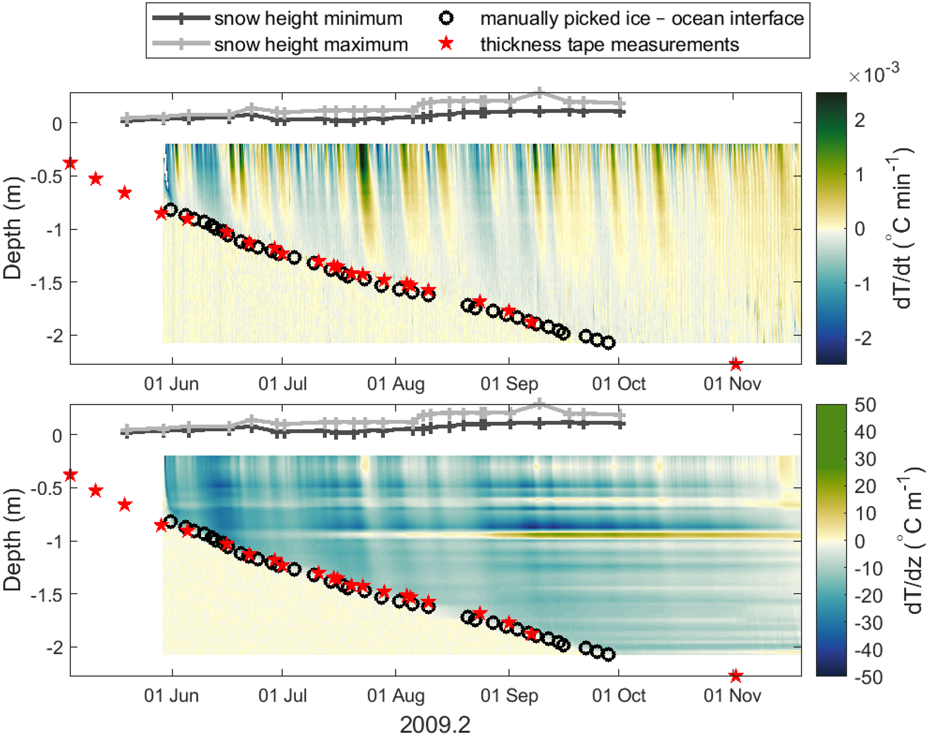
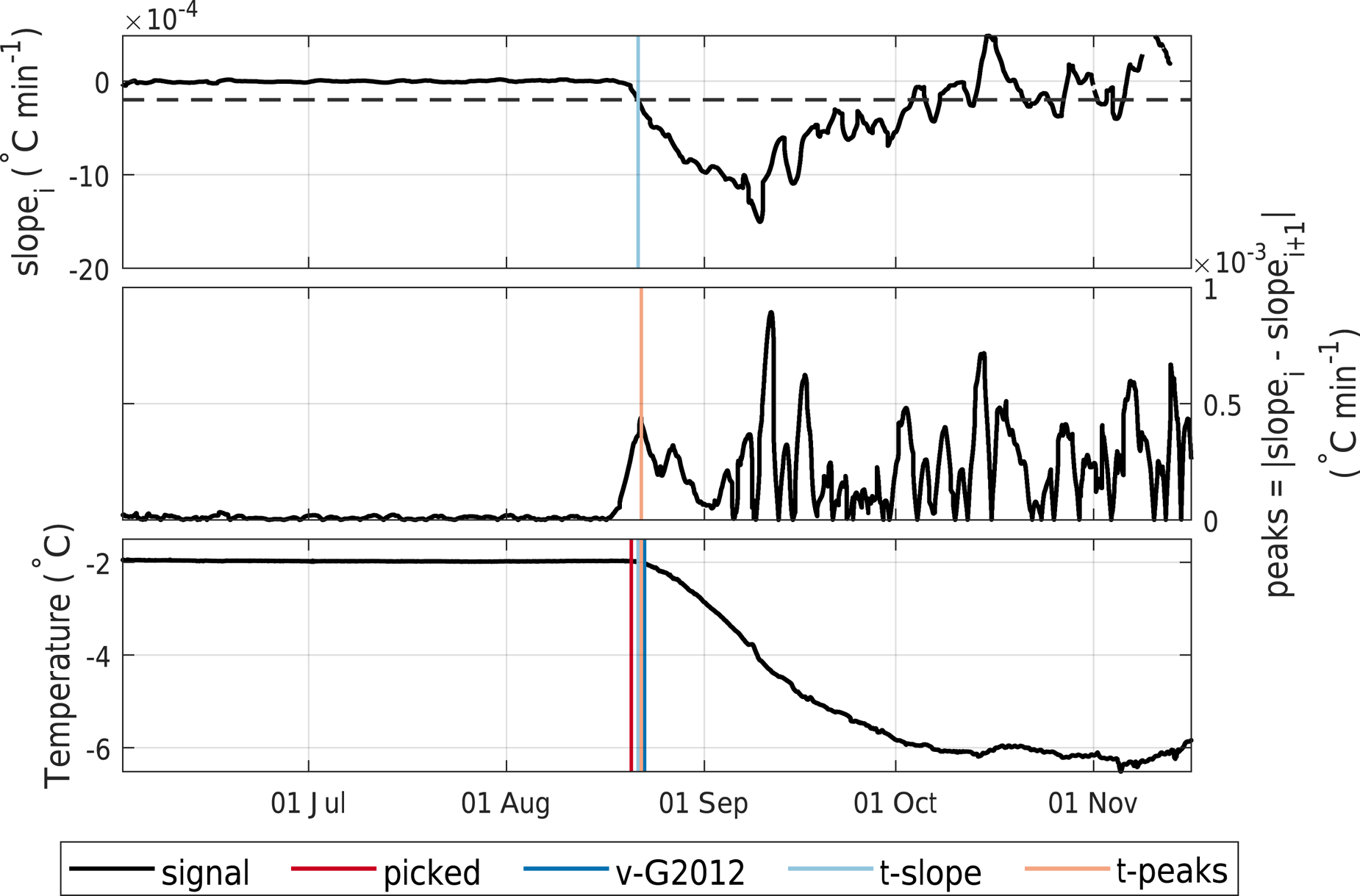
Temporal (top panel) and vertical (bottom panel) temperature gradient from a thermistor string deployed in 2009 in McMurdo Sound. Y-axis is depth through the ice in m, x-axis shows time and the colours correspond to the temperature gradient. Snow height, thickness tape measurements of and the manually picked location of the ice–ocean interface are shown as grey lines, red stars and black circles, respectively.
2.5.1. Estimating freeze-in from the vertical gradient (Method 2)
This is the method as described by Gough and others (Reference Gough2012) and referred to as v-G2012 henceforth. At each time step, the vertical temperature gradient over successive sets of four thermistors is calculated starting with the lowest four thermistors and moving upward until the gradient is more negative than the threshold of $-0.9^\circ$ C m−1. Once this threshold is reached, the intersection between the mean ocean temperature and the linear regression with depth of the temperature of the four thermistors is calculated. The intersection is taken to be the ice thickness and all thermistors are classed as ‘ice’ or ‘ocean’ according to their depth relative to this ice thickness (see Fig. 7). A new mean ocean temperature is then calculated from the thermistors classed as ‘ocean’. The resulting time series of sea-ice thicknesses is smoothed with a 7 d running mean and the time when the thickness exceeds the depth of a thermistor is chosen as the time this thermistor freezes in. Thus, v-G2012 not only gives freeze-in times for the thermistors, but also a continuous time series of the sea-ice thickness.
Ice–ocean interface as detected by Reference GoughGough and others's method from the vertical temperature gradient at each time step (v-G2012). Grey dots show temperature of thermistors classed as ‘ice’, blue dots show the temperature of the thermistors in the ocean. The ice–ocean interface is marked by the dashed black line. The plot shows the time when the thermistor at −1.715 m is found to freeze-in in the 2009.2 deployment, the same thermistor freeze-in as shown in Figure 8.

Freeze-in times (vertical lines) during the 2009.2 deployment as detected by the t-slope and t-peak methods. The Reference GoughGough and others’ method v-G2012, and the manually picked time for the thermistor at 1.715 m depth are also shown. The top panel shows the slope over the moving window (t-slope method) and the slope cut-off we use to find the freeze-in time (horizontal dashed line), the middle panel shows the absolute difference between the slope over neighbouring moving windows (t-peak method), the bottom panel shows the temperature of the thermistor.
2.5.2. Estimating freeze-in from the temporal gradient using t-slope and t-peak (Methods 3 and 4)
We calculated the temporal gradient of the temperature over a 3 d moving window and defined the freeze-in time of a thermistor as (a) the time when the slope first drops below a certain threshold (‘t-slope’ method, see top panel in Fig. 8) or (b) when the difference in slope between neighbouring windows is maximal (‘t-peak’ method, middle panel in Fig. 8). For the t-slope method we chose a slope cut-off of −2 × 10⁻⁵°C min−1 times the sample interval of the dataset in minutes. The t-peak method was examined using Matlab's findpeaks function which picks the first peak that has a certain height and prominence. The method queries different peak heights in turn, starting with the highest peaks and moving to lower peaks if there are none in the higher category. We chose three steps, with minimum peak heights of 4 × 10⁻⁵°C min−1, 1 × 10⁻⁵°C min−1 and 5 × 10⁻⁶°C min−1 multiplied by the sample interval in minutes and a minimum peak prominence of 1 × 10⁻⁵°C min−1, 5 × 10⁻⁶°C min−1 and 2 × 10⁻⁶°C min−1 multiplied by the sample interval in minutes. We will go into more detail on how to choose parameters for different datasets in the Discussion.
2.6. How we measure and compare the performance of the methods
When choosing a method there are a number of criteria with which to assess the performance. A method should be both accurate and precise, readily applicable to a wide variety of datasets, and computationally efficient. This is complicated by the fact that there are no concurrent, continuous and independent measurements of sea-ice thickness for most of our thermistor data, which means we often have no ‘true’ sea-ice thickness against which to compare accuracy. We solve this problem by using a linear interpolation of the manually picked sea-ice thickness as our ‘truth’ against which to compare the automated methods. In cases where independent measurements of sea-ice thickness exist, from thickness tape measurements or an acoustic altimeter, we can also use these for comparison. It needs to be noted that manually picked freeze-in dates are subjective and uncertainties depend on the sample frequency of the data. We compared the results produced by different members of our team and arrived at an estimate for the uncertainty of manual picking of ±0.3 d, for data sampled at a 10 min interval, our most common sample frequency. To assess precision, we would need repeat measurements which again are not available. To overcome this obstacle, we created 100 artificial realisations per dataset using loess smoothing and bootstrapping which are described in detail in Section 2.7 and in Appendix A. The methods for detecting freeze-in are applied to these repeats resulting in a distribution of freeze-in times. For each thermistor this freeze-in time distribution is compared to the manually picked freeze-in time and, where available, the thickness measured with a thickness tape. The mean of the absolute differences (MAD) between the distribution of bootstrapped freeze-in times and the ‘truth’ is the precision. The difference between the median of the distribution and the truth is the bias, which we take as an estimate of the accuracy of the method. We report the difference between a method and the ‘truth’ as the bias ± the MAD, where we note that the bias can be negative if the method underestimates sea-ice thickness. To retain information on the shape of the distribution, which is often highly skewed, we use the 25th and 75th percentiles of the distribution as the errorbars of the thickness and to calculate the errorbars of the sea-ice growth rate. To assess the robustness of the methods for a wide variety of datasets and to allow for comparison of methods between datasets, we use only minimal manual intervention in the methods and apply the same parameters to all data without tuning for individual datasets. Thus, all our results for accuracy and precision are worst case values and can be improved by adapting the methods to the characteristics of a particular dataset.
2.7. Loess smoothing and bootstrapping
Our time series data are not stationary, in fact, the point where the temperature variation changes, from isothermal in the ocean, to colder and more variable in the ice, is the very feature we are interested in. Thus, we assumed that there is an underlying ‘true’ time series which is overlain by instrument noise, which is also non-stationary. Following Wongpan (Reference Wongpan2018) we created this ‘true’ time series (shown in Fig. 4e) by smoothing the data using the loess smoothing method with a window width of 1000 min (~16 h) and tricubic weights to reduce outlier effects. We then calculated and bootstrapped the residual of the time series, that is the difference between the measured and the loess smoothed time series, with a block bootstrap method. This effectively ‘scrambles’ the noise of the time series by rearranging blocks of noise and then adds this scrambled noise back on to the smoothed data. Further information on the bootstrapping method can be found in Appendix A.
2.7.1. Sensitivity analysis of the methods
The effects of our choice of parameters are assessed by performing sensitivity tests on the 2009.2 data in McMurdo Sound, as this dataset has the largest number of thermistors that are observed to freeze-in and extensive concurrent thickness tape measurements. The results of the sensitivity tests are described in detail in Appendix B. Overall, the sensitivity tests described in Appendix B and shown in Figure 13 confirm that the parameters chosen for this study give the best overall performance and that small changes in the parameters do not strongly affect the results.
3. Results
Of the 20 thermistor probe datasets from McMurdo Sound, four could not be used for any of our automated methods: deployments with one or fewer thermistors observed to freeze-in (see Table 1) and the 2011 dataset, which was too noisy to successfully perform a bootstrap. Additionally, both t-slope and t-peak failed in the years marked as noisy in Table 1. v-G2012 was unable to find the ice–ocean interface in 2019 due to very low absolute vertical temperature gradients at the interface. In the case of the Utqiaġvik dataset all methods were able to identify at least some of the freeze-in events.
A method is deemed to be successful if a thermistor was detected as freezing in within ±0.3 d (the difference in manual picking by different observers) to ±3 d (the window width used for calculating t-slope and t-peak) of the manually picked freeze-in time of the thermistor. Results are shown in Table 3. For the McMurdo Sound dataset, the success rate is highest for t-peak followed by t-slope and v-G2012, although all lie within 3 percentage points of each other. For the Utqiaġvik dataset, the success rate is highest for v-G2012 followed by t-slope and t-peak, with the latter two much less successful than v-G2012, especially for the lower tolerance of ±0.3 h.
Percentage of picked freeze-in events correctly identified by the v-G2012, t-slope and t-peak methods within a margin of error of 0.3–3 d

Figures 9 and 10 show the median difference between the distribution of bootstrapped freeze-in times and the picked freeze-in times, and the same for the data itself, for McMurdo Sound and Utqiaġvik, respectively. This comparison shows a number of things. First, the (median) difference to picked freeze-in times is greater for the bootstrapped realisations than for the data. In both cases the differences are much larger for the measurements from Utqiaġvik (Fig. 10) than for those from McMurdo Sound. Second, for both temporal gradient methods (t-slope and t-peak) one year of the McMurdo Sound data (1996) and several of the Utqiaġvik datasets show increasing median differences between the bootstrapped realisations and the picked freeze-in time with increasing sea-ice thickness (Figs 9 and 10). Because the increase in temporal temperature slope (for t-slope), and peak height (for t-peak) at the freeze-in time of the thermistors is in general very pronounced, it is easy for the methods to detect. However, bootstrapping increases the noise in the signal before a thermistor freezes in, making falsely early freeze-in detection more common. This causes the underestimation of freeze-in time to increase with increasing deployment time and thus thickness. The v-G2012 method does not show such a pronounced effect (Fig. 10), an indication that v-G2012 is more robust. This is confirmed by the far higher success rate in identifying freeze-in events of v-G2012 for the Utqiaġvik data, being positioned 20–30 percentage points higher than the next best performing temporal method for tolerances of 0.3 d (Table 3), and the lower variability of the results as measured by the width of the bootstrapped freeze-in time distribution.
Results from the McMurdo Sound bootstrapped realisations and data. Left: Median difference to manually picked freeze-in times for the bootstrapped realisations (filled circles) and the original data (open circles) with respect to depth for each method. Right: Annual average median difference to manually picked freeze-in times for the bootstrapped realisations (filled circles) and the original data (open circles) with respect to year for each method. 25th and 75th percentiles are shown in grey. Note that very narrow distributions appear to not have quantiles shown and the axis scale change at ± 3 d marked by the dashed grey lines. The solid black line is at 0 d.
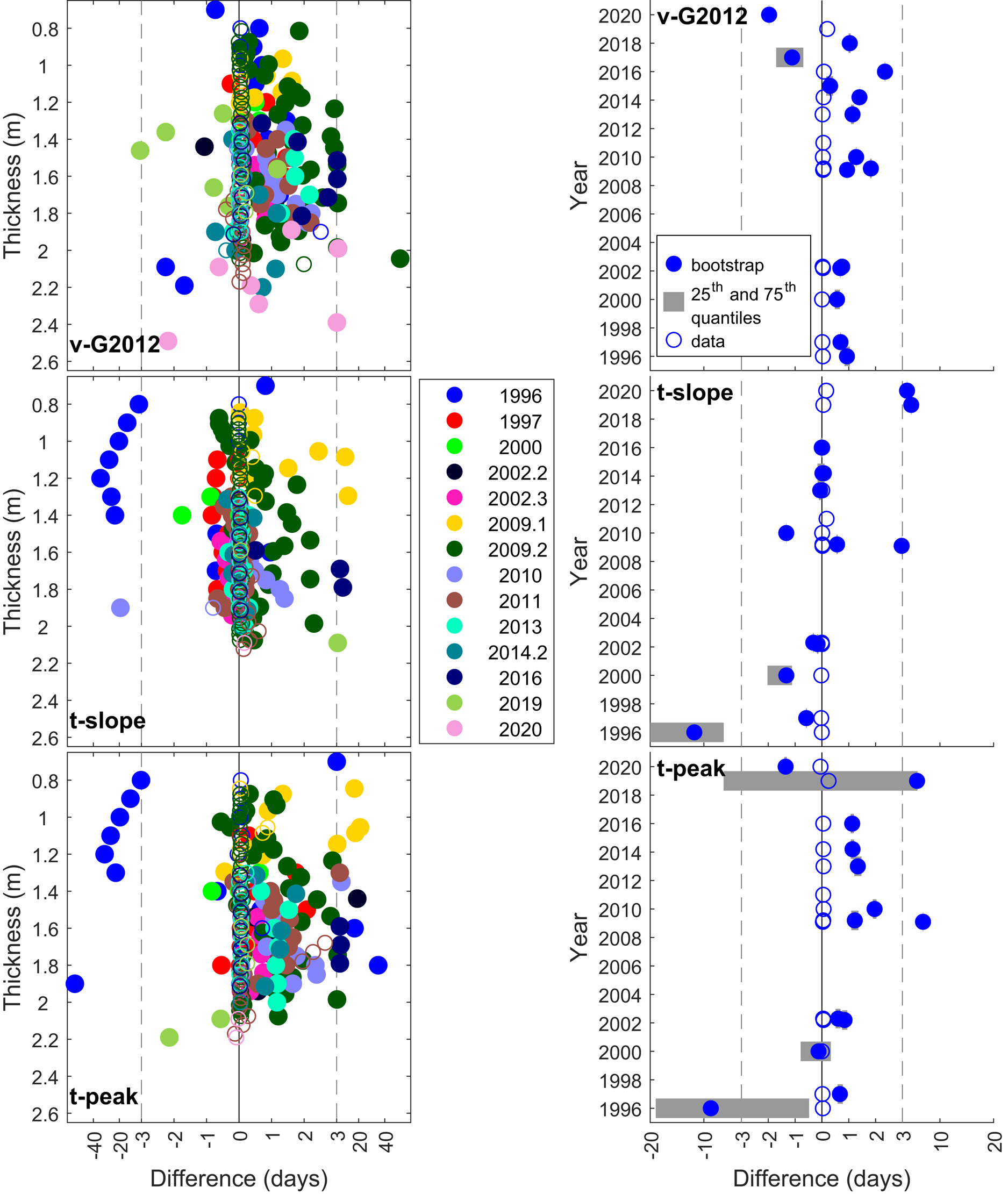
Results from the Utqiaġvik bootstrapped realisations and data. Left: Median difference to manually picked freeze-in times for the bootstrapped realisations (filled circles) and the original data (open circles) with respect to depth for each method. Right: Annual average median difference to manually picked freeze-in times for the bootstrapped realisations (filled circles) and the original data (open circles) with respect to year for each method. 25th and 75th percentiles are shown in grey. Note that very narrow distributions appear to not have quantiles shown and the axis scale change at ±3 d marked by the dashed grey lines. The solid black line is at 0 d.

Third, with the exception of the years in which the methods detect false early freeze-in times at the beginning of the record as described above (1996 McMurdo Sound data and, to different extents, 2007, 2012 – 2015 Utqiaġvik data), there is no change in median difference with increasing sea-ice thickness. Further, there does not appear to be a trend dependent on the year the data were collected. t-peak and v-G2012 skew towards identifying freeze-in events later than manual picking (resulting in lower sea-ice thickness) whereas t-slope is more evenly distributed.
Since the error derived from the bootstrapped realisations is neither an underestimate nor contains systematic errors with depth, we have confirmed that the bootstrap can be used to derive errors for individual freeze-in times and that the three automated methods can be applied to our data. In the following we will compare the thicknesses from all three automated methods to the picked thickness and to each other.
To illustrate the performance of the methods representative examples of the thicknesses, including errorbars, are shown in Figures 11a and 11b for data from 2009.2 and 2010 from the McMurdo Sound dataset, and for 2011 and 2013 from Utqiaġvik in Figures 12a and 12b, against thickness from thickness tapes and the acoustic altimeter. Here the freeze-in times (thicknesses) and growth rates are derived from the original data and the errorbars are the 25th and 75th quantiles of the distribution of freeze-in times from the bootstrap. In the case of the McMurdo Sound data, all methods plot very closely to each other and to the thickness measured using thickness tapes. To quantify the accuracy of the methods the results were linearly interpolated on to the same time vector and the difference to the picked thickness calculated. For each method the median difference and MAD of the thickness calculated from the original data to the picked thicknesses are shown in Table 4 and is below −1 ± 2 cm. For Utqiaġvik, the difference between methods and the errors of the methods is larger. In addition, it was not always possible to line up the acoustic altimeter, thickness tape and thermistor data-derived thicknesses, as seen in the 2013 data. The acoustic altimeter, though not biased towards the picked thickness by more than some of the thermistor string methods, shows a high MAD of 6 cm.
Thicknesses (top row) and growth rates (bottom row) for the 2009.2 (left column) and 2010 (right column) thermistor deployments in McMurdo Sound. Methods displayed are the v-G2012, t-slope and t-peak automated methods, manually picked freeze-in times and thickness tape measurements. Please note the break in scaling at the dashed horizontal line in the bottom row.

Thicknesses (top row) and growth rates (bottom row) for the 2011 (left column) and 2013 (right column) thermistor deployments at Utqiaġvik. Methods displayed are the v-G2012, t-slope and t-peak automated methods and manually picked freeze-in times alongside smoothed acoustic altimeter returns and thickness tape measurements. Please note the break in scaling at the dashed horizontal line in the bottom row. Shading is the 1 standard deviation of the smoothed acoustic altimeter-derived growth rates.

Median interpolated thickness and growth-rate differences and mean absolute difference (MAD) with respect to picked thicknesses and growth rates
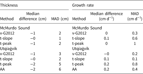
Negative values mean a lower thickness or growth rate than those calculated from the manually picked freeze-in times. AA is the acoustic altimeter.
To further gauge the precision of the automated methods against manual picking, we used the median variability in freeze-in time (the difference between the 25th and 75th percentiles) calculated from the bootstrapping and compared it to the variability in picked freeze-in times which we took to be 0.3 d. This confirmed that the variability in identified freeze-in times is lower for the automated methods than for manual picking for the McMurdo Sound data and lowest for v-G2012. In the case of the Utqiaġvik data the variability was the same for v-G2012 and manual picking and higher for the t-slope and t-peak methods. Thus, all automated methods have better precision than manual picking in McMurdo Sound and v-G2012 outperforms manual picking in the case of the Utqiaġvik data. Further, all automated methods produce reproducible results, which manual picking does not always do.
3.1. Growth rates
We calculate growth rates by applying the interface detection methods to the measured thermistor data, using the 25th and 75th percentiles of the distribution of the bootstrapped results for each individual thermistor to calculate error bounds. There is no significant difference in growth rate between the methods as evidenced by the mainly overlapping errorbars shown in Figures 11c and 11d for McMurdo Sound. In the case of the Utqiaġvik data, the errorbars overlap for the methods that successfully identify the ice–ocean interface, shown in Figures 12c and 12d. None of our thermistor-based methods were able to detect the negative growth rates during the melt season in Utqiaġvik detected by the acoustic altimeter (not shown). In general, all methods used show the same pattern in growth rate variability. This makes us confident that the variation in growth rate with time we see over a deployment is not an artefact of erroneous interface detection but a real signal. The automated methods show a lower variability in growth rate than the manual picking, especially visible where the vertical distance between thermistors is low, as in Figure 11c. It is interesting to note that overall there is a much lower variability in growth rates visible in our dataset from Utqiaġvik than in the growth rates from McMurdo Sound. The median difference and MAD of the growth rate from different methods are shown in Table 4 and is approximately 0 ± 1 cm d−1 for both McMurdo Sound and Utqiaġvik data.
3.2. Comparison to thickness tape data and acoustic altimeter returns
To get an independent measure of sea-ice thickness for comparison, we compared the calculated thicknesses to linearly interpolated thickness-tape measurements of sea-ice thickness. This was only possible for datasets where there was a minimum of three thickness tape measurements at times overlapping the time periods during which thermistors froze in. These datasets were 2009.2, 2014.2, 2015, 2018 and 2019 for McMurdo Sound and 2006–2010 for Utqiaġvik. The median difference and MAD of the automated freeze-in detection methods with respect to picked thicknesses were not significantly different for this subset of data compared to the entire dataset presented in Table 4. The median differences and MAD compared to tape measurements for all methods are shown in Table 5 with v-G2012 showing the lowest absolute median differences. On average, all methods slightly overestimate sea-ice thickness compared to the tape measure observations in McMurdo Sound by 2 ± 3 cm. For Utqiaġvik data, the opposite is true, and all methods underestimate sea-ice thickness compared to tape measurements by −8 ± 9 cm.
Median and mean absolute differences (MAD) of interpolated thicknesses with respect to thicknesses from tape measurements
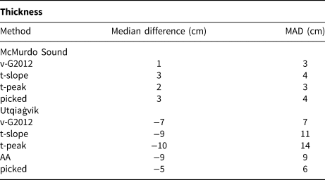
Negative values mean a lower thickness than from the tape measurements. AA is the acoustic altimeter.
As the acoustic altimeter at the Utqiaġvik site gives an independent, continuous measurement of the sea ice–ocean interface we can use it to further investigate the sea-ice thicknesses and growth rates at the Utqiaġvik site. The shape of the acoustic altimeter recorded sea-ice thickness curve matched the thicknesses derived from the thermistor data and is able to extend the observations into the melt season, something the thermistor methods are not capable of. Unfortunately, it was not always possible to align the acoustic altimeter-derived thicknesses with thickness tape measurements, sometimes leading to a difference between thickness tape, acoustic altimeter and thermistor-derived thicknesses of several centimetres (Fig. 12b). This may be due to imprecise measurement of the position of the acoustic altimeter relative to the ice–air interface at deployment, vertical movement of the probe in the latter part of the season due to preferential melting around the probe or inaccurate speed of sound corrections for temperature and salinity. Growth rates are not influenced by the absolute thickness and thus it is possible to compare the acoustic altimeter growth rates with those found by our analysis. Acoustic altimeter growth rates are highly variable which is why we calculated a 7 d moving average of the growth rate and the 1-standard deviation envelope. With few exceptions, all our methods yield growth rates within this envelope and close to the smoothed acoustic altimeter results (Figs 12c and 12d).
4. Discussion
4.1. The behaviour of the freeze-in detection methods
For datasets with near-constant ocean temperature at the freezing point and high growth rates (such as found in McMurdo Sound), the small differences in growth rates and thicknesses derived from the different methods studied here suggest that the choice of interface detection method has little influence on the analysis of the data. Precision (MAD) and accuracy (median difference) of all methods are better in the McMurdo Sound dataset than the Utqiaġvik dataset (Table 4).
The uncertainties in our methods lie within the range of uncertainties in sea-ice thicknesses derived from thermistor strings published in the literature and collected in Table 6. Overall, published uncertainties in sea-ice thickness from SIMS lie around 2 ± 3 cm. Comparing the thicknesses derived from v-G2012 to thickness tape measurements showed it is the most accurate method in the McMurdo Sound dataset and only slightly less accurate than manual picking in the Utqiaġvik dataset (see Table 5) where it nonetheless is the most successful and accurate choice of the automated interface detection methods studied here. Thus, our study indicates that it is possible to compare sea-ice thickness and growth rates derived from different thermistor probe designs and using different detection methods without incurring large errors.
Comparison of thickness precision from this study and the literature

Values for this study are median ± mean absolute difference between the interpolated thicknesses from all methods used in this study and thicknesses from manually picked freeze-in times. AA is the acoustic altimeter.
4.2. The differences between the Arctic and Antarctic datasets
In Utqiaġvik, the average growth rates over all methods, discarding obviously false values, decreased steeply over the course of the 3-month period from February to April from 0.8 ± 0.2 cm d−1 to 0.3 ± 0.2 cm d−1. In McMurdo Sound the growth rates remained almost constant over the equivalent period of August to October with average growth rates of 1 ± 0.4 cm d−1 to 0.7 ± 0.1 cm d−1. The higher growth rates in McMurdo Sound are known to be due to the presence of platelet ice because of the nearby McMurdo Ice Shelf and associated negative ocean heat fluxes (e.g., Smith and others, Reference Smith, Langhorne, Frew, Vennell and Haskell2012, Reference Smith2015), whereas the fast ice at Utqiaġvik has no platelet ice to maintain higher growth rates and may be subject to fluctuating and sometimes positive ocean heat fluxes (e.g., Smith and others, Reference Smith2016). In a warming climate, our results emphasise that the longevity of land-fast sea ice depends very specifically upon location and either detailed knowledge of regional growth processes, or in situ measurements, are needed to make predictions. This paper shows that all methods trialled here perform better for the McMurdo Sound data than for the Utqiaġvik data (Tables 3–5). In McMurdo Sound, the presence of ISW keeps the upper ocean at or just below the ocean freezing point. Further, for the data presented here, the sea ice is warmer and the growth rate lower off Utqiaġvik than in McMurdo Sound, meaning that the temporal gradient of the temperature of a thermistor at freeze-in is not as pronounced as in the McMurdo Sound dataset. Together with higher variability in ocean temperature this leads to v-G2012 and manual picking being the only methods to perform well on the Utqiaġvik data. A lower accuracy in ice–ocean interface detection with rising temperatures was also observed by Liao and others (Reference Liao2018). The detrimental effect of low growth rates on interface detection accuracy can also be seen in the 2019 and 2020 deployments in McMurdo Sound where the sea ice was relatively thick at deployment and the sea-ice growth rate low. An additional complication for the analysis of the Utqiaġvik datasets is that they reach into the melt season. Although some bottom melt is detected by the continuous record of ice–ocean interface location produced by v-G2012 (not shown), none of our methods are able to produce negative growth rates with accuracy. As mentioned by Perovich and others (Reference Perovich, Elder and Richter-Menge1997), during the melt season any vertical gradient method is limited by the fact that the temperature of the lower ice column approaches the ocean temperature, thus removing the change in temperature gradient at the interface. Bottom melt not only complicates the automated interface detection but also the manual picking of the interface. During these times the acoustic altimeter can provide valuable information on the evolution of the ice–ocean interface with near-real time, near-continuous measurements (Fig. 12a).
The dependence of all methods on correctly measuring the initial position of the sensors with respect to the ice–air or ice–snow interface is illustrated in Figure 12b where there is a discrepancy of several centimetres between the acoustic altimeter, thickness tape and thermistor-derived thicknesses in January. It is almost impossible to decide which of the different methods of measuring the sea-ice thickness shows the true thickness, although all show the same shape. Depending on the design of the SIMS used, the acoustic altimeter may measure sea-ice thickness at a slightly different location than the thermistor probe, adding an unknown spatial effect to the comparison. Furthermore, the location of the acoustic altimeter relative to the ice–air or ice–snow interface may vary over the season with the formation of superimposed ice or surface melt. In the case of no snow cover, this can be compensated for by using the distances measured by snow thickness sensors or by careful documentation of the location of the ice surface during station retrieval. The acoustic altimeter measurements additionally depend on accurate knowledge of the speed of sound in water, which is approximated from the ocean temperature. This approximation does not account for the influence of salinity on speed of sound. With possibly high variability in sea-water salinity under Arctic sea ice during the melt season, due to drainage of melt ponds (e.g., Martin and Kauffman, Reference Martin and Kauffman1974; Notz and others, Reference Notz2003), and during the sea-ice growth season due to advection of low salinity watermasses (e.g., Smith and others, Reference Smith2016), this cannot always be dismissed. Thus, although acoustic altimeters can provide valuable information in addition to a thermistor string, care is needed in the interpretation of the measurements. We correct the measurements taken off Utqiaġvik as much as possible for the effects of snow-ice/superimposed ice formation and surface ablation/preferential melting following the information given in Eicken and others (Reference Eicken2016). Surface ablation and snow-ice formation can be detected with thermistor strings (preferably with heating elements) extending from the ice into the snow pack and air. This was not the case for our McMurdo Sound deployments (where these effects are also not expected to contribute to ice mass balance during the time of our deployments) and is thus not investigated in detail here.
4.3. Choosing the right method for a dataset
Whether the vertical gradient or the temporal gradient of a dataset is the best choice to find the ice–ocean interface may depend on the characteristics of the dataset. The differences in accuracy (median difference) and precision (MAD) we have shown in Tables 3–5 are comparable only for good quality datasets. In datasets with noise or gaps the nature of these faults will dictate which method gives the most robust result.
Using a vertical gradient such as v-G2012 is insensitive to noise that is highly correlated in all thermistors and to step changes or temporal drift affecting the entire dataset. In cases where there are individual thermistors that have an offset, drift or noise different from the other thermistors in the chain, and where it is impractical to remove the affected thermistor from the dataset, using the temporal gradient will give better results. Choosing a temporal gradient method will prevent ‘bad’ thermistors from affecting the interface detection of neighbouring ‘good’ thermistors. However, all temporal gradient methods studied above (including manual picking) suffer from the fact that they only pick one change point per thermistor, if the first choice is wrong it needs to be manually adjusted. The vertical gradient method may also mis-assign the ice–ocean interface due to noise, but because it chooses an interface for each step in time, spikes in the interface due to bad choices can be easily smoothed out by applying a low-pass filter or moving mean as done by Gough and others (Reference Gough2012) and this study. The method described by Gough and others has the additional advantage that it produces a time series of ice–ocean interface locations, even between individual thermistors freezing in, giving a smoother result and higher temporal resolution. Further, it allows near-real time analysis of SIMS data which is of particular use for ice charts and logistics in ice infested waters.
The mis-identification of freeze-in events in this study is an over estimate, as we have not tuned any parameters to the individual datasets, rather choosing to apply the same values to all datasets to facilitate comparisons. Since both t-slope and t-peak are sensitive to the choice of parameters (Fig. 13), this naturally has an impact on our results that would not be seen if individual choices had been made for each year. The v-G2012 method is not as sensitive to choices in parameters (see Fig. 13) thus being more suited to application on a wide variety of datasets. If manual adjustments to freeze-in detection need to be made, it is helpful to plot the change in slope with time for the thermistors under investigation, as finding the point at which the change in slope is maximal is less subjective than examining the temperature or temperature slope alone (see Fig. 8).
Sensitivity tests of the v-G2012 (green), t-slope (black) and t-peak (blue) for the 2009.2 dataset. Precision (mean absolute difference, MAD) and bias (median difference) of the results compared to picked freeze-in times are shown for each changed parameter, the parameters used in this study are marked in bold. Dashed vertical lines note the scale break at ±3 d. Top-left panel shows the effect of changing the window width on which t-slope and t-peak operate; the top-right and bottom-right panels show the effect of varying the slope cut-off and the peak height (multiplying/dividing the base values by a factor 2), respectively; the bottom-left panel shows effects of varying the slope cut-off (sc), number of thermistors studied (N therm) and baseline ocean temperature (T ocean) assumed by v-G2012. The parameters used in this study (base) were: ${\rm sc} = -0.9^\circ$ C m−1, N therm = 4 and $T_{{\rm ocean}} = -1.9^\circ$
 C.
C.

Due to the limitations of our dataset, we were not able to investigate the behaviour of interface detection using thermal diffusivity proxy or methods that rely on air temperature, snow temperature profiles or ocean temperature calibration.
In addition to the data analysis presented here, the best possible results also depend on the thermistor string design. Following Pringle (Reference Pringle2004), we demonstrated the benefit of measuring standard resistors to reduce noise in the recorded data (Fig. 4), this can salvage otherwise unusable data. Close spacing (5 cm for thermistors in the 2009.2 probe), together with the high growth rate during the deployment, permitted high temporal variability in the measured thickness and growth rate to be resolved (Figs 11a and 11c). In 2019 and 2020 the late deployment of the probe in thick ice and the comparatively low growth rate (not shown) with a higher thermistor spacing (10 cm) led to only very few thermistors freezing in and thus also led to problems in calculating thickness and growth rate. We thus suggest a probe design that combines standard resistors in the wiring with a closer thermistor spacing (~3 cm in the lower part of the probe) to decrease measurement noise and increase the resolution towards the end of the growth season.
5. Summary and conclusion
The difference in sea-ice thickness and growth rate between different methods explored in this paper is within the associated uncertainties of these methods, ranging from (0 ± 1) cm to (− 2 ± 5) cm for thickness and (0.0 ± 0.3) cm d−1 to (0.2 ± 0.8) cm d−1 for growth rate (Table 4). This means that it is possible to compare sea-ice thicknesses derived from different methods and different thermistor string designs. This is confirmed by the range of error bounds given for other methods in the literature, summarised in Table 4, with values observed in our study lying within that range. The research gives confidence in the range of errors generally incurred for thickness and growth rate calculations and presents a method of calculating error bounds for specific observations without the need for repeat observations via bootstrapping. With these error bounds interannual variability can be distinguished from noise and future research will focus on the drivers for that variability.
Our research has shown that for datasets with high growth rates and vertical temperature gradients throughout the later part of the growth season (such as in McMurdo Sound, where growth rates lie between (1.0 ± 0.4) cm d−1 to (0.7 ± 0.1) cm d−1) the automated methods of ice–ocean interface detection from thermistor string data studied in this paper (v-G2012, t-slope and t-peak) perform better than manual picking (see Table 5). Further, manual methods suffer from subjective bias, can produce higher growth rate variability (Fig. 11c), are time intensive and even the same users are not able to consistently reproduce results. For datasets with lower growth rates and ice–ocean interface temperature gradients, especially in the later part of the growth season (such as at Utqiaġvik, where growth rates lie between (0.8 ± 0.2) cm d−1 to (0.3 ± 0.2) cm d−1 v-G2012 performs almost as well as manual picking (Table 5). We therefore argue that automated methods, with some manual adjustment, should be preferred over the more subjective and time-consuming manual interface detection. We show that v-G2012, the method published by Gough and others (Reference Gough2012), is the most robust and shows the highest success rates for the greatest range of data (>87 % for McMurdo Sound data and >63 % for Utqiaġvik data) of the methods studied here. It is influenced less by noise in the common components of a thermistor string and is less sensitive to parameter choices (Fig. 13). An additional advantage are the shorter computing times.
Acknowledgements
We acknowledge Joe Trodahl and MylesThayer for work on designing andbuilding the Otago/VUWdesignthermistor probes used in this study, and Peter Stroud, the late Richard Sparrow and Jim Woods for their assistance. Scott Base winter staff carried out deployment and maintenance. We acknowledge Marc Oggier for helpful discussions on the Arctic dataset and his assistance in accessing the data.
Data availability
The code used to loess filter the input data was adapted from Peter Green's R code, which he wrote whilst employed at the University of Otago. Alex Gough's method of defining the ice–ocean interface from thermistor data was developed whilst he was supported by a University of Otago Doctoral Scholarship. MER was supported by a University of Otago Doctoral Scholarship and the 2019 Antarctica New Zealand Sir Robin Irvine Scholarship. MER is grateful to the Polar Environments Research Theme at the University of Otago and NZARI for conference funding. Thermistor data collected in McMurdo Sound between 1996 and 2003 are available under https://drive.google.com/drive/folders/1ooUH9dPvWT66afFC51Cb0JOHg66rn0sy, data collected in 2002 and 2003 were part of the project ‘Measurements and Improved Parameterization of the Thermal Conductivity and Heat Flow through First-Year Sea Ice’, OPP-0126007*. Data collected in 2009, 2010 and 2013 are available at the data repository PANGAEA (Gough and others, Reference Gough2017; Smith and others, Reference Smith2017b, Reference Smith2017b; Gough and others, Reference Gough2017). The thermistor data in McMurdo Sound collected after 2009 were collected with the following funding and logistics support: IRL Subcontract to the University of Otago (2010, 2011); University of Otago Research Grants (2010, 2011, 2014, 2015 (Event Manager: Inga Smith)); NIWA subcontract to University of Otago, ‘Antarctic and High Latitude Climate’ (2013-2018); Contribution from MBIE-funded project ‘Antarctic sea ice thickness: harbinger of change in the Southern Ocean’ (2013 (PIs: Pat Langhorne and Wolfgang Rack)); Contribution from MBIE-funded Curious Minds public engagement project ‘Far from Frozen’ (2016, (leader: Craig Grant, Otago Museum)); US Fulbright Scholar Award (Cecilia Bitz, 2013); NZARI (2015 (PIs: Pat Langhorne and Craig Stevens), 2017, 2018 (PI: Greg Leonard)) Deep South National Science Challenge project TOPIMASI (2016–2018 (PI: Pat Langhorne)); Antarctic Science Platform Project 4 (Sea ice and carbon cycles) (2019, 2020 (Event Manager: Greg Leonard)); Marsden Fund project ‘Supercooling measurements under ice shelves’ (2020 (PI: Inga Smith)) and will be made available though PANGAEA. The thermistor data from the Arctic were collected as part of the Seasonal Ice Zone Observing Network (SIZONet) with funding from the National Science Foundation (OPP #0856867) and is available on the Arctic Data Centre under doi:10.18739/A2D08X (Eicken and others, Reference Eicken2016).
Author's contributions
MER processed and analysed the data and wrote the paper. GHL, IJS and PJL took a leading part in the running of the Otago SIMS programme, and provided feedback on the data processing and analysis. ARM took a leading part in the running of the UAF SIMS programme, and provided feedback on the Utqiaġvik dataset. MP helped with the statistics involved in bootstrapping and data analysis. All authors contributed to the final draft of the paper.
Appendix A. Bootstrapping
To create artificial ‘repeat’ observations of our time series we split our data into a ‘signal’ and a ‘noise’ component. The signal component is the loess smoothed data, as described in Section 2.7, and the noise is the difference between this and the data, the residual. We ‘scramble’ the noise using bootstrapping and add it back on to the ‘signal’ component to get 100 artificial repeat observations, the bootstrapped data. We chose a block bootstrap for our data as the data have correlation in both time and space and this correlation can be retained by using a block bootstrap. Block lengths were varied randomly to result in a geometric distribution around a mean of 5000 min (~3.5 d) since this method is less sensitive to the choice of block length than fixed length block bootstraps (Politis and Romano, Reference Politis and Romano1994). The average block length of 5000 min was chosen to be longer than the window we apply in our linear regression analysis (see description of t-slope and t-peak methods in Section 2.5.2), thus keeping the characteristics of the bootstrapped residual close to those of the original residual over the window. The auto-correlation length of the residual is in general much shorter than the average block length, though some datasets display auto-correlation up to lags higher than the block length. Since the geometric distribution has a high number of values lower than the mean of the distribution with a long tail to values higher than the mean, long auto-correlation lengths are included in the distribution of block lengths. No significant difference in our results was found for other choices of average blocklengths. Randomly located blocks of random length were combined to give a bootstrapped residual of the same length as the original residual. The bootstrapped residual was then added to the loess smoothed data to create a bootstrapped realisation of the data. This was repeated until we had a set of 100 realisations for each dataset. We only considered data intervals that did not have gaps wider than the smoothing window for both the smoothing and bootstrapping.
Appendix B. Sensitivity analysis
We performed sensitivity analysis to determine the effect of changes in our parameter choices for all methods on the results. Results from the sensitivity analysis are shown in Figure 13. We varied the parameters as follows. For the v-G2012 method (bottom-left panel): the number of thermistors (N therm) over which the slope in temperature with depth was calculated; the slope cut-off (sc) for this gradient; and the temperature of the ocean assumed for the first profile examined by the method (Tocean). For the t-slope and t-peak methods: the width of the window over which the slope in temperature with time was calculated (window width in days shown in the top-left panel); the slope cut-off for this gradient used in t-slope (top-right panel); and a factor with which we multiplied the peak height and peak prominence used for t-peak (bottom-right panel).
For the v-G2012 method, the greatest change was observed when changing the number of thermistors considered by the algorithm, with fewer thermistors leading to greater mean absolute differences (MAD) and median differences in the results. Changing the ocean temperature or slope cut-off had negligible effects on the results. For t-slope and t-peaks, window widths below 1 d caused the most extreme deterioration in median difference and MAD. With increasing window widths, the performance of t-slope improved, but the performance of t-peak decreased, leading to overall the lowest median difference and MAD values for the 3 d window used in our study (see top-left panel of Fig. 13). The slope cut-off chosen for t-slope produces the lowest median difference and MAD, with MAD increasing for both lower and higher values (see top-right panel of Fig. 13). In the case of the 2009.2 dataset, the median difference and MAD increase for higher peak heights in t-peak and decrease when reducing the peak height from the default (see bottom-right panel of Fig. 13). However, this is not true for all datasets, with the performance of the peak height chosen in this study producing the overall best results. Overall, the sensitivity tests shown in Figure 13 confirm that the parameters chosen for this study give the best overall performance and that small changes in the parameters do not strongly affect the results.


 Open access