


1. Introduction
During the COVID-19 pandemic, many governments recommended quarantine to those who had close contact with infected individuals for a certain period. The U.K. asked for 14 days of quarantine at the initial stage of the pandemic, which was shortened to 10 days in December 2020. The U.S. also began with 14 days of quarantine and lifted the recommended quarantine for vaccinated individuals in December 2021. Japan also started with 14 days of recommended quarantine, which was subsequently shortened to 10 days in January 2022, then to 7 days later that month, and to 5 days in July 2022.Footnote 1 Given its widespread use across countries, it is important for us to understand its benefits and costs in order to evaluate the efficacy of past policies and to design better policies in the future.
In this paper, we aim to shed light on the cost of the quarantine policy in the labor market by conducting a large-scale retrospective survey in Japan. In the survey, we asked quarantined workers how quarantine affected their labor outcomes. Using the data on quarantined workers, we first analyze summary statistics on hours worked and earnings during and after the quarantine period. We then perform regression analyses to understand which characteristics of workers are associated with negative labor outcomes. Finally, we estimate the reduction in the aggregate labor supply due to quarantine. Some quarantined workers turned out to be infected with COVID-19, while others were not. Throughout the analyses, we pay particular attention to the labor outcomes of uninfected quarantined workers after the quarantine period to see if quarantine had “scarring” effects independently of the health effects associated with COVID-19 symptoms.
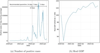
To provide context for our analysis, we show infection and economic outcomes during the COVID-19 pandemic in Japan in Figure 1. Panel (a) and (b) in the figure show the 7-day moving average of the number of positive cases and the real GDP normalized at 2020-Q1, respectively. Inside the left panel, we also show the recommended duration of quarantine mentioned earlier. According to the left panel, Japan was successful in containing the infection in 2020 and 2021. In 2022 – after the first two doses of vaccines were distributed to most citizens and once the Omicron variant became the main driver of infection – the number of new infections increased dramatically. According to the right panel, real GDP fell sharply in the second quarter of 2020, in line with the experiences of other countries during the COVID-19 pandemic. Real GDP recovered sharply in the third quarter of 2020 and continued its gradual recovery thereafter.
Number of positive cases and real GDP during the pandemic in Japan.

Figure 1. Long description
Two line graphs depict the number of positive cases and real GDP during the pandemic in Japan. The first graph shows the number of positive cases with a 7-day moving average from January 2020 to January 2023. The x-axis represents the date, and the y-axis represents the number of positive cases. The graph highlights recommended quarantine periods of 14 days, 10 days, 7 days, and 5 days. The second graph shows the real GDP from the first quarter of 2020 to the first quarter of 2023, with the x-axis representing the date and the y-axis representing the real GDP indexed to 100 in the first quarter of 2020. The first graph shows significant peaks in positive cases, particularly around 2022 and early 2023. The second graph shows a dip in real GDP in the first quarter of 2020, followed by a steady recovery and eventual increase above the baseline by the first quarter of 2023. All values are approximated.
We find that a large fraction of quarantined workers experienced reductions in daily hours worked or daily earnings during quarantine relative to their levels right before quarantine. $36$
% and
$36$
% and $23$
% of workers experienced reductions in daily hours worked and daily earnings, respectively, during quarantine. The average reduction in earnings during quarantine conditional on a reduction was
$23$
% of workers experienced reductions in daily hours worked and daily earnings, respectively, during quarantine. The average reduction in earnings during quarantine conditional on a reduction was $55$
%. For some workers, reductions in hours worked and earnings continued even after the quarantine period, albeit by a smaller degree.
$55$
%. For some workers, reductions in hours worked and earnings continued even after the quarantine period, albeit by a smaller degree. $15$
% of workers experienced a reduction in monthly hours after quarantine, and
$15$
% of workers experienced a reduction in monthly hours after quarantine, and $12$
% of workers experienced a reduction in monthly earnings after quarantine. The average reduction in earnings after quarantine conditional on a reduction was
$12$
% of workers experienced a reduction in monthly earnings after quarantine. The average reduction in earnings after quarantine conditional on a reduction was $38$
%. The reductions in hours and earnings after quarantine lasted for
$38$
%. The reductions in hours and earnings after quarantine lasted for $2.7$
months and
$2.7$
months and $3.5$
months, respectively, on average.
$3.5$
months, respectively, on average.
Reductions in hours and earnings after quarantine were observed not only for infected workers but also for uninfected workers. $33$
% and
$33$
% and $22$
% of uninfected workers experienced reductions in hours worked and earnings during the quarantine period, respectively.
$22$
% of uninfected workers experienced reductions in hours worked and earnings during the quarantine period, respectively. $13$
% and
$13$
% and $11$
% of uninfected workers experienced reductions in hours worked and earnings even after the quarantine period, respectively. The average duration of reductions in hours worked and earnings was
$11$
% of uninfected workers experienced reductions in hours worked and earnings even after the quarantine period, respectively. The average duration of reductions in hours worked and earnings was $3.0$
months and
$3.0$
months and $3.9$
months, respectively.
$3.9$
months, respectively.
Negative labor outcomes of infected quarantined workers likely capture the effects of both quarantine itself and possible symptoms associated with COVID-19 infection – symptoms known to be often persistent. However, negative labor outcomes of uninfected quarantined workers likely capture the pure effects of quarantine, independent of the effects associated with possible COVID-19 symptoms. The continuation of negative labor outcomes among uninfected quarantined workers after the quarantine period suggests the scar of quarantine. That is, quarantine had a persistent impact on hours worked and earnings independent of the persistent health effects associated with COVID-19 infection.
We argue that the observed reductions in hours and earnings are driven by the decline in labor supply rather than the decline in labor demand that plagued the economy throughout the pandemic. Ideally, we would like to have data on both quarantined and non-quarantined workers to compare their earnings and hours and purge out the effect of lower labor demand. However, we focus on quarantined workers and analyze their high-frequency changes in earnings and hours around quarantine. Collecting comparable data for non-quarantined workers would be challenging because that would require an additional survey and that survey would likely suffer from more severe recall-bias, as discussed in detail in Section 2. To assess the plausibility of our argument, we also compute the reductions in hours and earnings excluding months of presumably declining labor demand, such as periods of the state-of-emergency order. We find that the results are broadly the same as those from the full sample, consistent with our argument that the observed reductions in hours and earnings during and after quarantine are likely due to labor supply, as opposed to labor demand.
We find that non-regular workers, workers without remote work options, and workers in food–beverage–accommodation industries were more likely to experience reductions in hours worked and earnings and that these workers suffered a larger reduction in earnings on average if they did experience reduced earnings. These results hold both during and after the quarantine. Female workers were more likely to experience reduced hours than male workers during quarantine. Older workers were less likely to experience reductions in hours and earnings than younger workers during quarantine. Workers without children, more educated workers, and workers with higher income were less likely to experience a reduction in earnings than workers living with children, uneducated workers, and workers with lower income, respectively, both during and after quarantine.
At the aggregate level, we find that quarantine had a modest impact on aggregate hours in 2020 and 2021 but a sizable impact in 2022. The reduction in the aggregate hours worked attributable to quarantine of uninfected workers – relative to the aggregate hours in 2019 – was $0.06$
% in 2020,
$0.06$
% in 2020, $0.23$
% in 2021, and
$0.23$
% in 2021, and $0.98$
% in 2022. While the average reduction per uninfected quarantined worker declined over time, a spike in the number of uninfected quarantined workers pushed up the aggregate reduction in hours worked. More than three-quarters of the aggregate reduction in hours worked is due to the scar of quarantine, that is, the continued reduction in hours worked among uninfected quarantined workers.
$0.98$
% in 2022. While the average reduction per uninfected quarantined worker declined over time, a spike in the number of uninfected quarantined workers pushed up the aggregate reduction in hours worked. More than three-quarters of the aggregate reduction in hours worked is due to the scar of quarantine, that is, the continued reduction in hours worked among uninfected quarantined workers.
Our paper contributes to an extensive literature on labor market dynamics during the COVID-19 pandemic. This literature has examined various aspects of labor markets, including heterogeneous labor-market impacts (Alon et al. Reference Alon, Doepke, Olmstead-Rumsey and Tertilt2020; Coibion et al. Reference Coibion, Gorodnichenko and Weber2020; Albanesi and Kim, Reference Albanesi and Kim2021; Kikuchi et al. Reference Kikuchi, Kitao and Mikoshiba2021; Shibata, Reference Shibata2021; Alon et al. Reference Alon, Coskun, Doepke, Koll and Tertilt2022; Bluedorn et al. Reference Bluedorn, Caselli, Hansen, Shibata and Tavares2023; Cortes and Forsythe, Reference Cortes and Forsythe2023), remote work (Bartik et al. Reference Bartik, Bertrand, Lin, Rothstein and Unrath2020a; Deole et al. Reference Deole, Deter and Huang2023; Hansen et al. Reference Hansen, Lambert, Bloom, Davis, Sadun and Taska2023; Soh et al. Reference Soh, Oikonomou, Pizzinelli, Shibata and Tavares2025), reallocation and sectoral mismatch (Forsythe et al. Reference Forsythe, Kahn, Lange and Wiczer2022; Pizzinelli and Shibata, Reference Pizzinelli and Shibata2023), labor-market effects via infection (Fischer et al. Reference Fischer, Reade and Schmal2022; Goda and Soltas, Reference Goda and Soltas2022; Chiba et al. Reference Chiba, Hori, Nakata, Sasaki and Takaku2024), and the decline in the labor force participation rate (Faberman et al. Reference Faberman, Mueller and Şahin2022; Abraham and Rendell, Reference Abraham and Rendell2023; Lee et al. Reference Lee, Park and Shin2023).
Our paper is closely related to a set of studies aimed at understanding the effects of non-pharmaceutical interventions (NPIs) on labor markets. Some authors have examined the effect of lockdown policies – likely the most strict form of NPI in a pandemic – on labor market outcomes, often exploiting variations across time and space in policy. Such studies include, but are not limited to, Bartik et al. (Reference Bartik, Cullen, Glaeser, Luca and Stanton2020b), Baek et al. (Reference Baek, McCrory, Messer and Mui2021), Spiegel and Tookes (Reference Spiegel and Tookes2021), and Chetty et al. (Reference Chetty, Friedman and Stepner2024). Our paper differs from these papers because we focus on a different NPI – quarantine policy – and we conduct an original retrospective survey.
We complement the literature that analyzes the benefits of quarantine policy for reducing transmission.Footnote 2 This literature evaluates the efficacy of quarantine policies in mitigating the spread of the virus (see Sivaraman et al. (Reference Sivaraman, Dhawan, Chopra and Bhat2024) for review). As discussed earlier, however, it is important for policymakers to understand both the benefits and costs of quarantine policy in order to design better policies in the future. To our knowledge, our paper is the first to quantitatively investigate the negative impact of quarantine policy on labor outcomes the cost of quarantine policy.
Our analysis of the uninfected workers’ labor outcomes after the quarantine period is related to the literature on the scarring effects of negative shocks in the labor market. Many have empirically documented that recession and unemployment have long-lasting effects on earnings and employment (Kahn, Reference Kahn2010; Davis and von Wachter, Reference Davis and von Wachter2011; Yagan, Reference Yagan2019; Heathcote et al. Reference Heathcote, Perri and Violante2020; Jaimovich and Siu, Reference Jaimovich and Siu2020; Arellano-Bover, Reference Arellano-Bover2022). Some have examined, either empirically or theoretically, the scarring effects associated with the COVID-19 pandemic (Barrero et al. Reference Barrero, Bloom and Davis2023; Jackson and Ortego-Marti, Reference Jackson and Ortego-Marti2024). We add to this literature by documenting that even a very short disruption in the labor market – quarantine typically lasted less than two weeks – can have persistent effects on labor outcomes.
This paper is organized as follows. Section 2 describes the survey design. Section 3 discusses summary statistics on labor outcomes following quarantine. Section 4 discusses regression analysis to understand the type of individuals who are more likely to experience the scar. Section 5 discusses the aggregate reduction in labor supply associated with quarantine policy. Section 6 discusses caveats of this paper. Section 7 concludes.
2. Survey and data
We conducted a large-scale retrospective survey in Tokyo from February 14, 2023 to February 21, 2023 to collect data on hours worked and earnings surrounding the quarantine period.
We collected the participants with the help of Cross Marketing Inc., an online marketing company in Japan.Footnote 3 The company has access to a pool of individuals interested in participating in various surveys. They can earn “points” that can be used for future expenditures upon completion of each survey.Footnote 4 Randomly selected individuals residing in Tokyo and aged between 20 and 64 years old were contacted with a targeted number of responses for each five-year interval age and sex set to match the age and sex distribution from the Population Census.
Among the collected participants who agreed to the survey guidelines, we conducted a screening survey to identify those who had close contact with individuals infected with COVID-19 and who had a job in March 2020.Footnote 5
If a participant satisfied these two criteria, the respondent proceeded to the main survey. We asked various questions regarding (i) demographic/socio-economic characteristics, (ii) job/employment characteristics, (iii) labor outcomes since the quarantine began, and (iv) other information.
For demographic/socio-economic characteristics, we asked presence of a partner (including spouse), presence of children – defined as children in college or below – and elderly – defined as a person aged 65 or more – in a household, worker’s education, and income of the respondent and his/her partner.
For job/employment characteristics, we asked the type of employment (regular employee, non-regular employee, self-employment/freelance, family business, or others), availability of remote work (at least partially available or not available), and industry.
For the labor outcomes, we asked a total of 8 questions. Three questions were about the labor outcomes during the quarantine period: (i) whether daily hours worked during quarantine changed from the level just before quarantine; (ii) whether daily earnings changed from the level just before quarantine; and (iii) if the answer to the second question is yes, the magnitude of the earnings reduction as a percentage of the pre-quarantine level. Note that, if a respondent had multiple experiences of quarantine due to close contact during the COVID-19 pandemic, the respondent answers an outcome of his/her first experience.Footnote 6
Five questions were about the labor outcomes after the quarantine period: (i) whether monthly hours worked after the quarantine changed relative to the level just before quarantine; (ii) whether monthly earnings changed after the quarantine relative to the level just before quarantine; (iii) if the answer to the first question is yes, the duration of the reduction in hours worked (in months); if the answer to the second question is yes, (iv) the magnitude of the earnings reduction as a percentage of the pre-quarantine level and (v) the duration of the earnings reduction (in months).
Summary statistics of demographic/family/employment characteristics

Table 1. Long description
The table presents summary statistics of demographic, family, and employment characteristics for the years 2020 to 2023. It includes data on the number of samples, average age, share of male, share of living with spouse or partner, share of living with elderly, share of living with children, share of college or more education, average income, partner’s average income, share of non-regular employees, share of remote work available workers, and average duration of quarantine. The table has 12 rows and 6 columns, with each row representing a different variable and each column representing a different year. Notable trends include a slight increase in average age from 42.5 in 2020 to 43.6 in 2023, a decrease in the share of male from 54.9 percentage in 2020 to 45.8 percentage in 2023, and a fluctuation in the share of living with children, with a low of 32.6 percentage in 2020 and a high of 44.9 percentage in 2022. The share of college or more education remains relatively stable around 62.9 percentage to 67.1 percentage. Average income and partner’s average income show minor variations, with incomes ranging from 4.0 million yen to 4.5 million yen. The share of non-regular employees slightly increases from 21.9 percentage in 2020 to 25.2 percentage in 2023. The share of remote work available workers peaks at 56.0 percentage in 2020 and drops to 46.5 percentage in 2023. The average duration of quarantine decreases from 10.3 days in 2021 to 6.0 days in 2023.
For “other information,” we asked; when the quarantine began; how many days the quarantine lasted; whether the respondent took a COVID-19 test after being exposed to an infected person; their test results if they were tested – that is, whether they were infected with COVID-19.
Note that we asked changes in daily hours and earnings during the quarantine period and changes in monthly hours and earnings after the quarantine period relative to the level right before the quarantine began. With this nature of our questions that ask changes within a short period of time, these reported reductions in hours worked and earnings likely reflect the effects of quarantine, as opposed to the effects related to the low labor demand during the pandemic.
The total number of responses completing the main questions is 7,998.Footnote 7 There were two responses with 999 days of quarantine, and we removed the two responses from the samples throughout the analysis.
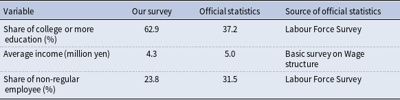
Table 1 shows summary statistics for key variables from our survey. The average age is $42.8$
.
$42.8$
. $66.8$
% of respondents lived with their spouse/partner,
$66.8$
% of respondents lived with their spouse/partner, $12.7$
% lived with elderly(s) where elderly refers to someone aged 65 or more, and
$12.7$
% lived with elderly(s) where elderly refers to someone aged 65 or more, and $42.5$
% lived with child(ren) where children include infants and primary-school, secondary-school, high-school, and college students. The share of workers with college or more education is
$42.5$
% lived with child(ren) where children include infants and primary-school, secondary-school, high-school, and college students. The share of workers with college or more education is $63$
% in our survey, substantially larger than the number from the Labour Force Survey –
$63$
% in our survey, substantially larger than the number from the Labour Force Survey – $37.2$
% among workers aged 15 to 64. The average earnings of respondents are
$37.2$
% among workers aged 15 to 64. The average earnings of respondents are $4.3$
million yen, and those of partners are also
$4.3$
million yen, and those of partners are also $4.3$
million yen. According to the Basic Survey on Wage Structure, the average annual earnings of workers aged 20 to 64 over 2020 to 2023 are
$4.3$
million yen. According to the Basic Survey on Wage Structure, the average annual earnings of workers aged 20 to 64 over 2020 to 2023 are $5.0$
million yen. The share of non-regular employees is
$5.0$
million yen. The share of non-regular employees is $23.8$
%. Our survey features a smaller share of non-regular employees relative to the share of non-regular employees during 2020–2023 with age 15 to 64 from the Labour Force Survey –
$23.8$
%. Our survey features a smaller share of non-regular employees relative to the share of non-regular employees during 2020–2023 with age 15 to 64 from the Labour Force Survey – $31.5$
%. The discrepancy in earnings and non-regular employee share between our survey and each official statistics – higher earnings and lower non-regular employee share in our survey – likely reflects the larger share of college-educated workers in our survey. These demographic and socioeconomic distributions are relatively stable over time. For easier comparison, Table 2 reports selected statistics from our survey and official statistics along with their sources.
$31.5$
%. The discrepancy in earnings and non-regular employee share between our survey and each official statistics – higher earnings and lower non-regular employee share in our survey – likely reflects the larger share of college-educated workers in our survey. These demographic and socioeconomic distributions are relatively stable over time. For easier comparison, Table 2 reports selected statistics from our survey and official statistics along with their sources.
Comparison of our survey and official statistics for 2020–2023

Table 2. Long description
The table presents a comparison of key variables from a survey and official statistics for the years 2020-2023. It includes three columns: Our survey, Official statistics, and Source of official statistics. The variables compared are the share of college or more education, average income, and the share of non-regular employees. The table has three rows for these variables. The share of college or more education is 62.9 percentage in our survey and 37.2 percentage in the official statistics, sourced from the Labour Force Survey. The average income is 4.3 million yen in our survey and 5.0 million yen in the official statistics, sourced from the Basic survey on Wage structure. The share of non-regular employees is 23.8 percentage in our survey and 31.5 percentage in the official statistics, sourced from the Labour Force Survey. The table highlights discrepancies between the survey data and official statistics, with higher education levels and lower non-regular employment in the survey data.
The sample sizes increase over time. The sample sizes are $574$
, 1,274, and 5,606 in 2020, 2021, and 2022, respectively. The numbers of infections in our sample are
$574$
, 1,274, and 5,606 in 2020, 2021, and 2022, respectively. The numbers of infections in our sample are $2.2$
and
$2.2$
and $9.8$
in 2021 and 2022, respectively, relative to 2020. This increasing pattern is qualitatively consistent with the increasing pattern in the number of infections. According to the Ministry of Health, Labour and Welfare, the numbers of infections are 60,312, 383,060, and 3,987,922 in 2020, 2021, and 2022, respectively. The numbers of infections are
$9.8$
in 2021 and 2022, respectively, relative to 2020. This increasing pattern is qualitatively consistent with the increasing pattern in the number of infections. According to the Ministry of Health, Labour and Welfare, the numbers of infections are 60,312, 383,060, and 3,987,922 in 2020, 2021, and 2022, respectively. The numbers of infections are $6.4$
and
$6.4$
and $66.1$
in 2021 and 2022, respectively, relative to 2020. Note that the number for 2023 is small because our survey took place in February: Our survey only covers information about quarantines that occurred in January and early February in 2023.
$66.1$
in 2021 and 2022, respectively, relative to 2020. Note that the number for 2023 is small because our survey took place in February: Our survey only covers information about quarantines that occurred in January and early February in 2023.
3. Labor outcomes during and after quarantine
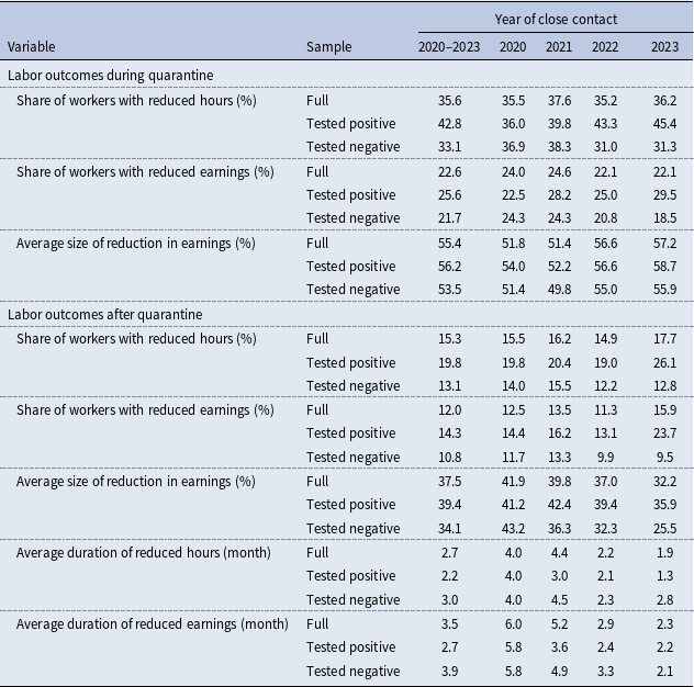
Table 3 presents summary statistics on labor outcomes during and after quarantine. We compute these statistics with full samples, samples of workers tested positive, and samples of workers tested negative. The statistics are computed for 2020–2023, as well as for each year.
From 2020 to 2023, $35.6$
% and
$35.6$
% and $22.6$
% of quarantined workers experienced reductions in hours and earnings, respectively. The average reduction in earnings was
$22.6$
% of quarantined workers experienced reductions in hours and earnings, respectively. The average reduction in earnings was $55.4$
% conditional on a reduction. In other words, nearly a quarter of workers lost more than half of their pre-quarantine earnings on average.
$55.4$
% conditional on a reduction. In other words, nearly a quarter of workers lost more than half of their pre-quarantine earnings on average.
Reductions in hours and earnings were observed even after the quarantine period was over. $15.3$
% and
$15.3$
% and $12.0$
% of quarantined workers continued to suffer reductions in hours and earnings, respectively, after the quarantine period. The reduction in earnings was
$12.0$
% of quarantined workers continued to suffer reductions in hours and earnings, respectively, after the quarantine period. The reduction in earnings was $37.5$
% on average. The reduction in hours and earnings lasted for
$37.5$
% on average. The reduction in hours and earnings lasted for $2.7$
months and
$2.7$
months and $3.5$
months, respectively. In other words, more than 10% of workers suffered in the labor market for nearly a quarter after quarantine.
$3.5$
months, respectively. In other words, more than 10% of workers suffered in the labor market for nearly a quarter after quarantine.
Summary statistics of labor outcomes

Table 3. Long description
The table presents summary statistics of labor outcomes during and after quarantine, segmented by full samples, workers tested positive, and workers tested negative. The data spans from 2020 to 2023, with specific breakdowns for each year. Key metrics include the share of workers with reduced hours and earnings, average size of reduction in earnings, and average duration of reduced hours and earnings. Notable trends show variations in labor outcomes based on test results and years, highlighting the impact of quarantine on different worker groups.
Note: The average size of reduction in earnings and the average duration of reduced earnings are conditional on reduced earnings, and the average duration of reduced hours is conditional on reduced hours.
The likelihood of reductions in hours worked and earnings as well as the size of the reduction in earnings remained relatively stable over time. However, the duration of reductions in hours and earnings became noticeably shorter over time: The duration of the reduction in hours declined from $4.0$
months in 2020 to
$4.0$
months in 2020 to $1.9$
months in 2023. The duration of the reduction in earnings declined from
$1.9$
months in 2023. The duration of the reduction in earnings declined from $6.0$
months in 2020 to
$6.0$
months in 2020 to $2.3$
months in 2023.
$2.3$
months in 2023.
Importantly, even uninfected quarantined workers – those workers tested negative – experienced a persistent reduction in hours and earnings. $13.1$
% and
$13.1$
% and $10.8$
% of uninfected quarantined workers had reductions in hours and earnings after quarantine, respectively.Footnote
8
The average reduction in earnings was
$10.8$
% of uninfected quarantined workers had reductions in hours and earnings after quarantine, respectively.Footnote
8
The average reduction in earnings was $34.1$
%. The reduction in hours and earnings lasted for
$34.1$
%. The reduction in hours and earnings lasted for $3.0$
months and
$3.0$
months and $3.9$
months on average, respectively. This result indicates that quarantine had persistent negative effects on hours and earnings independent of the negative health effects associated with COVID-19 infection – such health effects are also known to be persistent and often referred to as “Long COVID.” We call this persistent negative impact on labor outcomes for uninfected quarantined workers “the scar of quarantine.”
$3.9$
months on average, respectively. This result indicates that quarantine had persistent negative effects on hours and earnings independent of the negative health effects associated with COVID-19 infection – such health effects are also known to be persistent and often referred to as “Long COVID.” We call this persistent negative impact on labor outcomes for uninfected quarantined workers “the scar of quarantine.”
The duration and the size of the scar – the duration and the size of reduction in hours and earnings for uninfected quarantined workers – declined over time. The duration of hours reduction declined from $4.0$
months in 2020 to
$4.0$
months in 2020 to $1.3$
months in 2023. The duration of earnings reduction declined from
$1.3$
months in 2023. The duration of earnings reduction declined from $5.8$
months in 2020 to
$5.8$
months in 2020 to $2.1$
months in 2023. The size of the earnings reduction was
$2.1$
months in 2023. The size of the earnings reduction was $43.2$
% in 2020 and
$43.2$
% in 2020 and $25.5$
% in 2023. The likelihood of the reduction after quarantine remained relatively stable over time for uninfected workers. The likelihood of reduction in hours and earnings varied from
$25.5$
% in 2023. The likelihood of the reduction after quarantine remained relatively stable over time for uninfected workers. The likelihood of reduction in hours and earnings varied from $14.0$
% in 2020 to
$14.0$
% in 2020 to $12.8$
% in 2023 and from
$12.8$
% in 2023 and from $11.7$
% in 2020 to
$11.7$
% in 2020 to $9.5$
% in 2023, respectively.
$9.5$
% in 2023, respectively.
As we have discussed in Section 2, our survey has a larger share of college-educated workers than official statistics. To check the robustness of our finding in this section, we adjust the difference in the share of college-educated workers in Online Appendix A and we provide adjusted numbers in Online Appendix Table A1. More specifically, we compute averages using the share of educated workers from Labour Force Survey as opposed to the one from our survey. Even after the adjustment, our findings are broadly the same. A similar share of workers experienced reduction in hours and earnings with a similar size of earnings reduction. Also, workers experienced reductions in hours and earnings even after quarantine.
3.1 Labor supply or labor demand?
For each quarantined worker, we collect his/her labor market outcomes around the time of quarantine to estimate the effects of quarantine. Another way to estimate the effect of quarantine on labor supply would be to collect both quarantined and non-quarantined workers to compare their earnings and hours and purge out the effect of lower labor demand.
However, such data collection for non-quarantined workers would require conducting another survey. To collect data for non-quarantined workers, we would need to first collect days of quarantine by conducting a survey like ours and then conduct another survey that asks hours and earnings of non-quarantined workers around those days. Also, in the second hypothetical survey, the days being asked would be just random days for non-quarantined workers. It is unlikely that non-quarantined workers would recall their hours and earnings on those specific days. Due to these challenges, we focused on quarantined workers and analyzed their high-frequency changes in earnings and hours around quarantine – presumably a very memorable event for quarantined workers.
Nevertheless, some readers may wonder to what extent the reductions in hours and earnings presented in Table 3 are truly driven by labor supply rather than labor demand. To address this concern, we recompute summary statistics after excluding samples from the months (1) when a state of emergency was declared, (2) when Indices of Tertiary Industry Activity (ITA) declined compared with the previous month, or (3) when ITA for accommodations and restaurants (ITA-AR) declined compared with the previous month. These months likely correspond to times when labor demand was declining. By excluding these periods, we can assess whether hours and earnings were reduced to the same degree even during months with rising labor demand. The corresponding summary statistics– parallel to those in Table 3 – are presented in Online Appendix B as Online Appendix Table A2, Table A3, and Table A4.
The tables show that the main patterns remain unchanged after excluding the samples from these months. From 2020 to 2023, $33.1$
–
$33.1$
– $35.0$
% and
$35.0$
% and $21.8$
–
$21.8$
– $22.0$
% of quarantined workers experienced reductions in hours and earnings, respectively, during quarantine. The average reduction in earnings was
$22.0$
% of quarantined workers experienced reductions in hours and earnings, respectively, during quarantine. The average reduction in earnings was $53.5$
–
$53.5$
– $55.4$
% conditional on a reduction.
$55.4$
% conditional on a reduction. $15.0$
–
$15.0$
– $15.4$
% and
$15.4$
% and $11.0$
–
$11.0$
– $11.9$
% of quarantined workers continued to suffer reductions in hours and earnings, respectively, after the quarantine period. The reduction in earnings after the quarantine period was
$11.9$
% of quarantined workers continued to suffer reductions in hours and earnings, respectively, after the quarantine period. The reduction in earnings after the quarantine period was $35.2$
–
$35.2$
– $37.2$
% on average. The reduction in hours and earnings lasted for
$37.2$
% on average. The reduction in hours and earnings lasted for $2.3$
–
$2.3$
– $2.7$
months and
$2.7$
months and $3.0$
–
$3.0$
– $3.7$
months, respectively.
$3.7$
months, respectively.
For the scar, $12.6$
–
$12.6$
– $13.4$
% and
$13.4$
% and $9.7$
–
$9.7$
– $10.7$
% of uninfected quarantined workers had reductions in hours and earnings after quarantine, respectively. The average reduction in earnings was
$10.7$
% of uninfected quarantined workers had reductions in hours and earnings after quarantine, respectively. The average reduction in earnings was $33.2$
–
$33.2$
– $33.4$
%. The reduction in hours and earnings lasted for
$33.4$
%. The reduction in hours and earnings lasted for $2.6$
–
$2.6$
– $2.9$
months and
$2.9$
months and $3.3$
–
$3.3$
– $3.9$
months on average, respectively.
$3.9$
months on average, respectively.
Thus, even when focusing on months with stable or increasing labor demand, we continue to observe comparable declines in hours and earnings. The observed reductions in hours and earnings during and after quarantine were likely to be driven by labor supply factors, as opposed to labor demand factors.
4. Heterogeneity in labor outcomes during and after quarantine
The previous section established that a sizable fraction of workers experienced reductions in hours worked and earnings during and after the quarantine period. In this section, we use regression analysis to study what types of workers are more likely to experience such negative labor outcomes.
4.1 Specification
We analyze how labor outcomes are related to workers’ characteristics using a simple OLS regression:
 \begin{align*} y_{i}=\boldsymbol{\beta }'\mathbf{x}_{i}+\epsilon _{i}, \end{align*}
where $y_{i}$
is an outcome variable of individual
$y_{i}$
is an outcome variable of individual $i$
,
$i$
, $\mathbf{x}_{i}$
is a vector of characteristics of individual
$\mathbf{x}_{i}$
is a vector of characteristics of individual $i$
,
$i$
, $\boldsymbol{\beta }$
is a vector of coefficients on each characteristic, and
$\boldsymbol{\beta }$
is a vector of coefficients on each characteristic, and $\epsilon _{i}$
is a disturbance term.
$\epsilon _{i}$
is a disturbance term.
For outcome variables, we consider the eight statistics – three during the quarantine period and five after the quarantine period – discussed in the previous section.
The worker’s characteristics, $\mathbf{x}_{i}$
, include the following variables. For household characteristics, we have a dummy for female, a dummy for older age group (40 or more), a dummy for college education. For socioeconomic characteristics, we have a dummy for living with elderly, a dummy for living with kids, a dummy for higher income (four million yen or more), a dummy for having a partner/spouse with lower income (between zero and four million yen), a dummy for having a partner/spouse with higher income (four million yen or more). For job characteristics, we have a dummy for non-regular employee, a dummy for remote work option availability, dummies for raw material sector, manufacturing sectors, and food–beverage–accommodation sector.Footnote
9
Other variables are a dummy for tested positive, a dummy for test not taken, a dummy for longer quarantine (8 days or more), and dummies for month–year fixed effect.
$\mathbf{x}_{i}$
, include the following variables. For household characteristics, we have a dummy for female, a dummy for older age group (40 or more), a dummy for college education. For socioeconomic characteristics, we have a dummy for living with elderly, a dummy for living with kids, a dummy for higher income (four million yen or more), a dummy for having a partner/spouse with lower income (between zero and four million yen), a dummy for having a partner/spouse with higher income (four million yen or more). For job characteristics, we have a dummy for non-regular employee, a dummy for remote work option availability, dummies for raw material sector, manufacturing sectors, and food–beverage–accommodation sector.Footnote
9
Other variables are a dummy for tested positive, a dummy for test not taken, a dummy for longer quarantine (8 days or more), and dummies for month–year fixed effect.
4.2 Results
4.2.1 Characteristics related to hours and earnings during quarantine
Table 4 presents the regression results for the three labor outcome variables during quarantine. The first, second, and third columns are the results for reduction in hours, reduction in earnings, and the size of earnings reduction (conditional on reduced earnings), respectively. Since the dependent variables are reduction dummies and the size of earnings reduction, positive coefficients mean negative labor outcomes.
Estimated coefficients from the regression of labor outcomes during quarantine

Table 4. Long description
The table presents regression results for three labor outcome variables during quarantine. It includes three columns: reduction in hours, reduction in earnings, and the size of earnings reduction. The table has 16 rows, each representing different demographic and employment factors such as sex, age, education level, living arrangements, income levels, employment status, remote work availability, industry type, test results, and quarantine duration. Each row shows the estimated coefficients for the reduction dummy variables and the size of earnings reduction. Positive coefficients indicate negative labor outcomes. Notable trends include significant impacts for non-regular employees, those with remote work availability, and those in the food-beverage-accommodation industry. The table also highlights the number of observations and R-squared values for each regression model.
Note: Displaying estimated coefficients for selected variables with their industry-clustered standard errors in parentheses. Positive coefficients mean negative labor outcomes. Statistical significance is indicated by * at the 10% level, * * at the 5% level, and * * * at the 1% level.
Some demographic and socioeconomic characteristics were associated with labor outcomes in a statistically significant way. Female workers were $5.0$
percentage point more likely to experience a reduction in hours than male workers. Female workers had an earnings reduction
$5.0$
percentage point more likely to experience a reduction in hours than male workers. Female workers had an earnings reduction $5.4$
percentage point larger than male workers did. Older workers were
$5.4$
percentage point larger than male workers did. Older workers were $3.3$
percentage point and
$3.3$
percentage point and $3.1$
percentage point less likely to experience a reduction in hours and earnings, respectively, than younger workers. Workers with a college degree or higher were
$3.1$
percentage point less likely to experience a reduction in hours and earnings, respectively, than younger workers. Workers with a college degree or higher were $2.3$
percentage point less likely to face reduced earnings than workers without a college degree. Workers living with children faced
$2.3$
percentage point less likely to face reduced earnings than workers without a college degree. Workers living with children faced $2.8$
and
$2.8$
and $3.0$
percentage point higher likelihoods of hours and earnings reduction, respectively. Workers with higher income were
$3.0$
percentage point higher likelihoods of hours and earnings reduction, respectively. Workers with higher income were $8.2$
percentage point less likely to experience a reduction in earnings than workers with lower income.
$8.2$
percentage point less likely to experience a reduction in earnings than workers with lower income.
Job characteristics – non-regular vs. regular, remote work availability, and industry – were associated with the labor outcomes during quarantine in a statistically significant and quantitatively important way. Non-regular employees were $6.8$
percentage point and
$6.8$
percentage point and $21.7$
percentage point more likely to experience reductions in hours and earnings, respectively, than regular employees. Non-regular employees faced
$21.7$
percentage point more likely to experience reductions in hours and earnings, respectively, than regular employees. Non-regular employees faced $20.9$
percentage point larger reduction in earnings than regular employees did. Workers with remote work options were
$20.9$
percentage point larger reduction in earnings than regular employees did. Workers with remote work options were $23.2$
percentage point and
$23.2$
percentage point and $15.3$
percentage point less likely to experience the reduction in hours and earnings, respectively, than workers without remote work options. Workers with remote work options faced
$15.3$
percentage point less likely to experience the reduction in hours and earnings, respectively, than workers without remote work options. Workers with remote work options faced $16.0$
percentage point smaller reduction in earnings than workers without remote work option did. Workers in food–beverage–accommodation industries were
$16.0$
percentage point smaller reduction in earnings than workers without remote work option did. Workers in food–beverage–accommodation industries were $6.6$
percentage point and
$6.6$
percentage point and $5.4$
percentage point more likely to experience a reduction in hours and earnings than workers in the service sector, respectively. Workers in food–beverage–accommodation industries faced
$5.4$
percentage point more likely to experience a reduction in hours and earnings than workers in the service sector, respectively. Workers in food–beverage–accommodation industries faced $3.5$
percentage point larger reduction in earnings than workers in the service sector did.
$3.5$
percentage point larger reduction in earnings than workers in the service sector did.
The test outcome and quarantine duration were associated with some labor outcomes in a statistically significant way. Workers tested positive were $8.7$
percentage point and
$8.7$
percentage point and $1.7$
percentage point more likely to experience reductions in hours worked and earnings, respectively, than workers tested negative. Workers experienced a reduction in hours
$1.7$
percentage point more likely to experience reductions in hours worked and earnings, respectively, than workers tested negative. Workers experienced a reduction in hours $6.4$
percentage point more likely and a reduction in earnings
$6.4$
percentage point more likely and a reduction in earnings $6.6$
percentage point more likely when quarantine was longer than a week than when quarantine was a week or shorter.
$6.6$
percentage point more likely when quarantine was longer than a week than when quarantine was a week or shorter.
4.2.2 Characteristics related to hours and earnings after quarantine
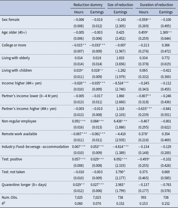
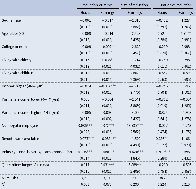
Table 5 presents the regression results with the labor outcomes after quarantine. As in Table 4, the first, second, and third columns are the results for reduction in hours, reduction in earnings, and the size of earnings reduction (conditional on reduced earnings), respectively. The fourth and fifth columns are the duration of reductions in hours and earnings. As in Table 4, positive coefficients mean negative labor outcomes.
Estimated coefficients from the regression of labor outcomes after quarantine

Table 5. Long description
The table presents regression coefficients for various labor outcomes after quarantine. It includes five columns: reduction dummy in hours and earnings, size of reduction in earnings, and duration of reduction in hours and earnings. Each row represents different variables such as sex, age, education level, living arrangements, income levels, employment type, remote work availability, industry, test results, and quarantine duration. The coefficients indicate the impact on labor outcomes, with positive coefficients signifying negative labor outcomes. Notable trends include significant impacts for non-regular employees, those in the food-beverage-accommodation industry, and individuals with positive test results.
Note: Displaying estimated coefficients for selected variables with their industry-clustered standard errors in parentheses. Positive coefficients mean negative labor outcomes. Statistical significance is indicated by * at the 10% level, * * at the 5% level, and * * * at the 1% level.
Some demographic and socioeconomic characteristics were associated with some labor outcomes after quarantine in a statistically significant way. Female workers faced $0.60$
months shorter duration of reduction in hours than male workers. Older workers experienced
$0.60$
months shorter duration of reduction in hours than male workers. Older workers experienced $1.37$
months longer reduction in earnings than younger workers. Workers with a college degree or higher were
$1.37$
months longer reduction in earnings than younger workers. Workers with a college degree or higher were $1.5$
percentage point and
$1.5$
percentage point and $3.3$
percentage point less likely to experience reduction in hours and earnings, respectively, than workers without a college degree.
$3.3$
percentage point less likely to experience reduction in hours and earnings, respectively, than workers without a college degree.
Workers with higher income were $2.0$
percentage point less likely to experience hours reduction and
$2.0$
percentage point less likely to experience hours reduction and $3.5$
percentage point less likely to experience an earnings reduction than workers with lower income. Workers with higher income experienced
$3.5$
percentage point less likely to experience an earnings reduction than workers with lower income. Workers with higher income experienced $8.5$
percentage point smaller reduction in earnings than workers with lower income. Workers faced
$8.5$
percentage point smaller reduction in earnings than workers with lower income. Workers faced $0.81$
months and
$0.81$
months and $0.64$
months shorter duration of reduction in hours when their partner’s income was less than four million yen and when their partner’s income was more than four million yen, respectively, than when a worker had no partner. Workers’ household member composition – living with children or elderly – had no statistically significant relation to labor outcomes.
$0.64$
months shorter duration of reduction in hours when their partner’s income was less than four million yen and when their partner’s income was more than four million yen, respectively, than when a worker had no partner. Workers’ household member composition – living with children or elderly – had no statistically significant relation to labor outcomes.
Job characteristics were related to some labor outcomes after quarantine in a statistically significant and quantitatively important way. Non-regular employees were $9.1$
percentage point and
$9.1$
percentage point and $8.4$
percentage point more likely to experience reductions in hours and earnings, respectively, than regular employees. Non-regular employees faced an earnings reduction that was
$8.4$
percentage point more likely to experience reductions in hours and earnings, respectively, than regular employees. Non-regular employees faced an earnings reduction that was $6.4$
percentage point larger than regular employees did. Workers with remote work option were
$6.4$
percentage point larger than regular employees did. Workers with remote work option were $6.7$
percentage point and
$6.7$
percentage point and $6.1$
percentage point less likely to experience reductions in hours and earnings, respectively, than those without remote work option. Workers in food–beverage–accommodation industry were
$6.1$
percentage point less likely to experience reductions in hours and earnings, respectively, than those without remote work option. Workers in food–beverage–accommodation industry were $6.7$
percentage point and
$6.7$
percentage point and $5.3$
percentage point more likely to experience hours and earnings reduction, respectively, than those in the service sector. Workers in food–beverage–accommodation industry faced
$5.3$
percentage point more likely to experience hours and earnings reduction, respectively, than those in the service sector. Workers in food–beverage–accommodation industry faced $4.8$
percentage point smaller reduction in earnings than those in the service sector did. These job characteristics were overall not associated with the duration outcomes in a statistically significant way.
$4.8$
percentage point smaller reduction in earnings than those in the service sector did. These job characteristics were overall not associated with the duration outcomes in a statistically significant way.
Test outcomes and duration of quarantine were also associated with some labor outcomes in a statistically significant way. Workers tested positive were $5.7$
percentage point and
$5.7$
percentage point and $2.9$
percentage point more likely to experience reductions in hours and earnings, respectively, than workers tested negative. Workers tested positive faced
$2.9$
percentage point more likely to experience reductions in hours and earnings, respectively, than workers tested negative. Workers tested positive faced $6.1$
percentage point larger earnings reduction than workers tested negative did. The likelihood of hours reduction was
$6.1$
percentage point larger earnings reduction than workers tested negative did. The likelihood of hours reduction was $2.9$
percentage point higher when quarantine was of longer duration (longer than seven days) than when quarantine was of short duration (within seven days).
$2.9$
percentage point higher when quarantine was of longer duration (longer than seven days) than when quarantine was of short duration (within seven days).
There are a few interesting results worth discussing. First, workers with remote work option experienced a reduction in hours for a longer duration (by $0.38$
months) than workers without remote work option, even though they were less likely to experience declines in hours and earnings. Some workers with remote work option likely switched from in-person work to remote work during quarantine and may have kept working remotely after quarantine. When working remotely, they may be able to choose their working hours more flexibly. As a result, workers who hoped for shorter working hours may start choosing shorter hours after quarantine.
$0.38$
months) than workers without remote work option, even though they were less likely to experience declines in hours and earnings. Some workers with remote work option likely switched from in-person work to remote work during quarantine and may have kept working remotely after quarantine. When working remotely, they may be able to choose their working hours more flexibly. As a result, workers who hoped for shorter working hours may start choosing shorter hours after quarantine.
Second, workers tested positive experienced reduction in hours for a shorter duration (by $0.50$
months). Workers were more likely to be tested positive if their jobs required face-to-face communication with other colleagues and customers. Jobs with frequent human interactions may not allow flexibility in terms of working hours. If so, the duration of reduction in hours worked would be short-lived.
$0.50$
months). Workers were more likely to be tested positive if their jobs required face-to-face communication with other colleagues and customers. Jobs with frequent human interactions may not allow flexibility in terms of working hours. If so, the duration of reduction in hours worked would be short-lived.
4.2.3 Characteristics related to scar (Hours and earnings of tested negative after quarantine)
We now analyze heterogeneity in the scarring effects of quarantine. For that purpose, we run regressions with labor outcomes after quarantine using only the sample of uninfected workers – workers tested negative. The estimated coefficients are presented in Table 6.
Estimated coefficients from the regression of labor outcomes after quarantine with samples of workers tested negative

Table 6. Long description
The table presents estimated coefficients from a regression analysis of labor outcomes after quarantine, focusing on workers who tested negative. It includes data on the reduction in hours and earnings, the size of the reduction in earnings, and the duration of the reduction in both hours and earnings. The table has 14 rows and 9 columns, with columns labeled Reduction dummy, Size of reduction, and Duration of reduction, each further divided into Hours and Earnings. Key variables include sex, age, education level, living arrangements, income levels, employment status, remote work availability, industry, and quarantine duration. Notable trends include significant reductions in earnings for higher-income individuals and those in the food-beverage-accommodation industry, as well as the impact of remote work availability on reducing the duration of earnings reduction.
Note: Displaying estimated coefficients for selected variables with their industry-clustered standard errors in parentheses. Positive coefficients mean negative labor outcomes. Statistical significance is indicated by * at the 10% level, * * at the 5% level, and * * * at the 1% level.
Some demographic and socioeconomic characteristics were related to some aspects of the scar, though the relations are typically weaker than what we have seen in Tables 4 and 5. Uninfected workers with college or more education were $2.9$
percentage point less likely to experience a reduction in earnings than uninfected workers without college education. Uninfected workers with higher own income were
$2.9$
percentage point less likely to experience a reduction in earnings than uninfected workers without college education. Uninfected workers with higher own income were $3.7$
percentage point less likely to experience a reduction in earnings than uninfected workers with lower own income. Sex, age, living with children or elderly, the existence of a partner, and partner’s earnings were not associated with the outcome variables in a statistically significant way.
$3.7$
percentage point less likely to experience a reduction in earnings than uninfected workers with lower own income. Sex, age, living with children or elderly, the existence of a partner, and partner’s earnings were not associated with the outcome variables in a statistically significant way.
Job characteristics were associated with some of the labor outcomes of uninfected workers in a statistically significant and quantitatively important way, as in the previous subsection. That is, among uninfected workers, non-regular workers, workers without remote work options, and workers in food–beverage–accommodation industries were more likely to experience reductions in hours worked and earnings.
Quarantine duration was also associated with some of the labor outcomes of uninfected workers in a statistically significant and quantitatively important way, as in the previous subsection. Workers with longer quarantine were $3.1$
percentage point more likely to experience a reduction in earnings than workers with shorter quarantine, with
$3.1$
percentage point more likely to experience a reduction in earnings than workers with shorter quarantine, with $5.9$
percentage point larger reduction.
$5.9$
percentage point larger reduction.
5. Macroeconomic impact
In this section, we estimate the reduction in aggregate hours associated with quarantine in Japan.
5.1 Estimation procedure
First, we estimate the average reduction in hours for each year of quarantine, industry, and test outcomes from our survey. We begin by splitting the entire sample into sub-samples based on the year of quarantine, industry, and test outcomes. For each sub-sample, we estimate the likelihood of reduction in hours for both during and after quarantine. To obtain the average reduction of hours, we multiply it by the product of average size of earnings reduction during/after quarantine conditional on reduction – substitute for the size of reduction in hours conditional on reduction because our data does not have information on the size of hours reduction – and the average duration of quarantine/hours reduction.
Second, we compute the average reduction in hours for each year of quarantine and test outcomes. To this end, we take the average over industries of the average reduction for each year of quarantine, industry, and test outcomes obtained in the previous step, using industry-wise employment from the Population Census as weights to aggregate across industries. By this procedure of taking industry-wise employment weighted average, we can match our samples to data in terms of the distribution of workers’ industry, which is not matched in our survey design.
Third, we compute average reduction per quarantined worker for each year by aggregating over the test outcomes. In computing the average reduction caused by quarantine, it is not clear if the reduction of hours for tested positive is due to quarantine or infection. We attribute all of their reductions to infection because the reduction in hours for workers tested positive in our paper is smaller than the average reduction of hours due to infection in Chiba et al. (Reference Chiba, Hori, Nakata, Sasaki and Takaku2024). Thus, we set the hours reduction for workers tested positive to zero.
Finally, we obtain the aggregate reduction due to quarantine by multiplying the average reduction per quarantined worker by the number of close contacts within workers. We estimate the number of close contacts within workers by multiplying $5.35$
by the estimated number of positive cases within workers. This is based on a survey conducted in a city in Toyama,Footnote
10
which showed that there are a total of 530 close contacts for 99 infected people, meaning
$5.35$
by the estimated number of positive cases within workers. This is based on a survey conducted in a city in Toyama,Footnote
10
which showed that there are a total of 530 close contacts for 99 infected people, meaning $5.35$
close contacts were recorded per infection. The number of positive cases within workers is estimated by combining data on the number of positive cases with ages between 20 to 69 from the Ministry of Health, Labour, and Welfare and the labor force participation rate within age 15 to 64 from Labour Force Survey.
$5.35$
close contacts were recorded per infection. The number of positive cases within workers is estimated by combining data on the number of positive cases with ages between 20 to 69 from the Ministry of Health, Labour, and Welfare and the labor force participation rate within age 15 to 64 from Labour Force Survey.
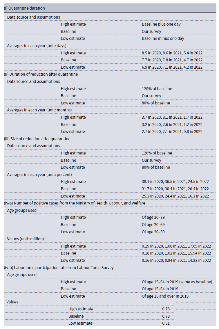
In addition to the baseline scenario, we compute the reduction in aggregate hours under two different scenarios to take into account uncertainties associated with various assumptions in the baseline calculation. In one scenario, we provide a low estimate on the reduction by assuming (i) one day shorter quarantine duration, (ii) a month shorter duration of hours reduction after quarantine, (iii) average hours reduction during and after quarantine 20% smaller than the average earnings reduction, and (iv) fewer cases of quarantine obtained from data of (iv-a) the number of positive cases between age 20 to 59 and (iv-b) the labor force participation rate of age 15 or more. In the other scenario, we provide a high estimate on the reduction by assuming (i) one day longer quarantine duration, (ii) a month longer duration of hours reduction after quarantine, (iii) the size of hours reduction during and after quarantine 20% larger than the ones of earnings, and (iv) larger cases of quarantine obtained from data of (iv-a) the number of positive cases between age 20 to 79 and (iv-b) the labor force participation rate within age 15 and 64 (same as the baseline). Table 7 summarizes these assumptions.
Data source in benchmark and assumptions in low estimate and high estimate scenarios

Table 7 Long description
The table has four sections: Quarantine duration, Duration of reduction after quarantine, Size of reduction after quarantine, and Number of positive cases from the Ministry of Health, Labour, and Welfare. Each section includes data source and assumptions, followed by averages in each year for high estimate, baseline, and low estimate. The table has 14 rows and 4 columns. Row 1: Data source and assumptions. Row 2: High estimate, Baseline plus one day. Row 3: Baseline, Our survey. Row 4: Low estimate, Baseline minus one day. Row 5: Averages in each year (unit: days). Row 6: High estimate, 8.5 in 2020, 8.6 in 2021, 5.4 in 2022. Row 7: Baseline, 7.7 in 2020, 7.8 in 2021, 4.7 in 2022. Row 8: Low estimate, 6.9 in 2020, 7.1 in 2021, 4.2 in 2022. Row 9: Data source and assumptions. Row 10: High estimate, 120 percent of baseline. Row 11: Baseline, Our survey. Row 12: Low estimate, 80 percent of baseline. Row 13: Averages in each year (unit: months). Row 14: High estimate, 3.7 in 2020, 3.1 in 2021, 1.7 in 2022. Row 15: Baseline, 3.2 in 2020, 2.6 in 2021, 1.2 in 2022. Row 16: Low estimate, 2.7 in 2020, 2.1 in 2021, 0.8 in 2022. Row 17: Data source and assumptions. Row 18: High estimate, 120 percent of baseline. Row 19: Baseline, Our survey. Row 20: Low estimate, 80 percent of baseline. Row 21: Averages in each year (unit: percent). Row 22: High estimate, 38.1 in 2020, 36.5 in 2021, 24.5 in 2022. Row 23: Baseline, 31.7 in 2020, 30.4 in 2021, 20.4 in 2022. Row 24: Low estimate, 25.3 in 2020, 24.4 in 2021, 16.3 in 2022. Row 25: Age groups used. Row 26: High estimate, Of age 20 to 79. Row 27: Baseline, Of age 20 to 69. Row 28: Low estimate, Of age 20 to 59. Row 29: Values (unit: million). Row 30: High estimate, 0.19 in 2020, 1.08 in 2021, 17.09 in 2022. Row 31: Baseline, 0.18 in 2020, 1.02 in 2021, 15.94 in 2022. Row 32: Low estimate, 0.16 in 2020, 0.94 in 2021, 14.33 in 2022. Row 33: Age groups used. Row 34: High estimate, Of age 15 to 64 in 2019 (same as baseline). Row 35: Baseline, Of age 15 to 64 in 2019. Row 36: Low estimate, Of age 15 and over in 2019. Row 37: Values. Row 38: High estimate, 0.78. Row 39: Baseline, 0.78. Row 40: Low estimate, 0.61.
Note: The numbers in the first three rows show averages over industries and test outcomes. When we compute the averages, quarantine duration, duration of reduction after quarantine, and the size of reduction during/after quarantine for workers tested positive are set to zero, as is consistent with the procedure in Section 5.1. Due to this method of averaging, the differences in the average quarantine duration across scenarios are less than one day, and the differences in the average duration of reduction after quarantine across scenarios are less than one month.
5.2 Results
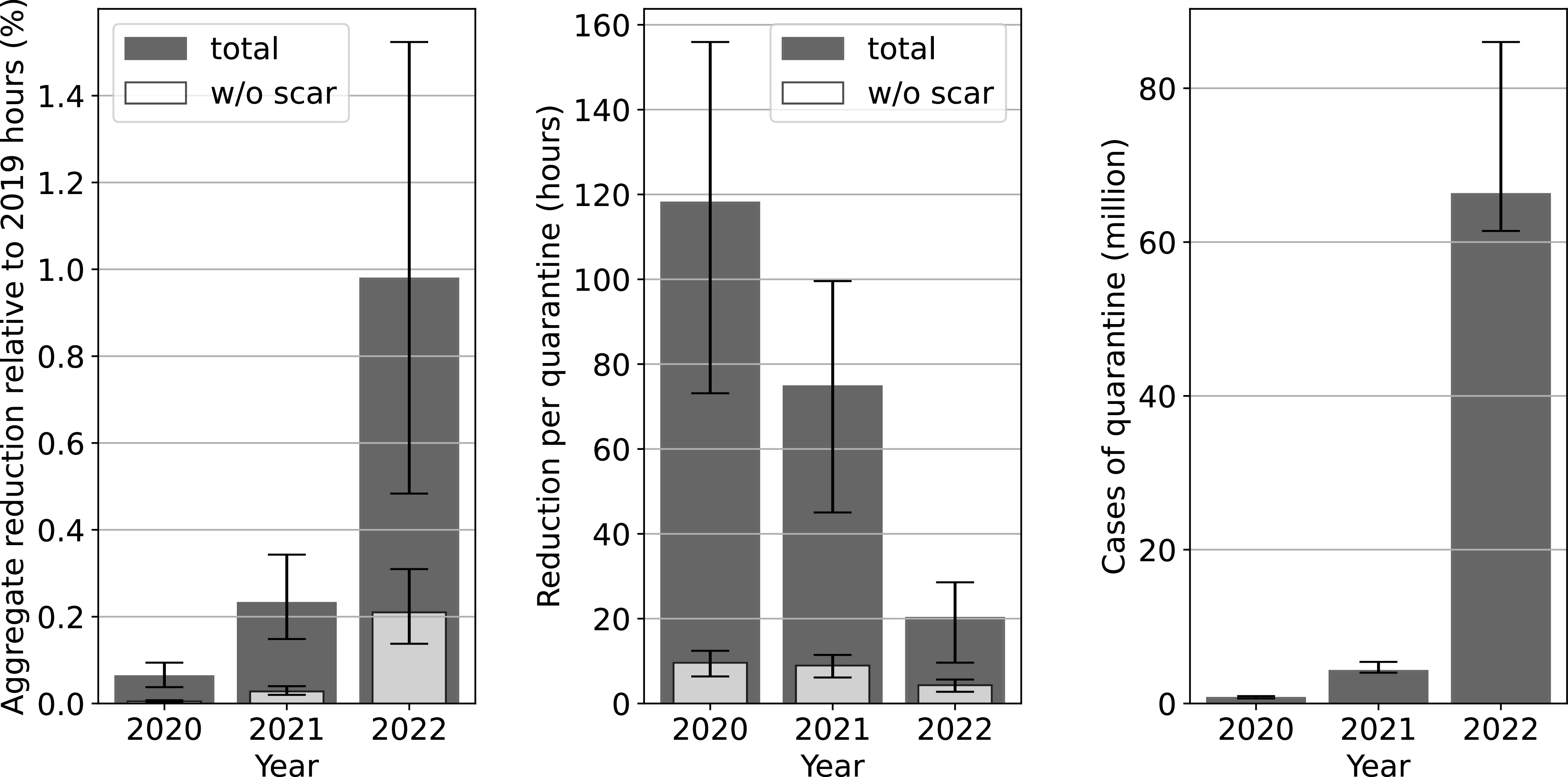
We plot the aggregate hours reduction of 2020, 2021, and 2022 in the left panel of Figure 2 as black bars. In the figure, we plot them relative to the aggregate hours in 2019. The upper and lower ends of the band represent the estimated reduction from the two alternative scenarios. According to the left panel, the aggregate reduction in hours due to quarantine was modest in 2020 and 2021 but sizable in 2022. The aggregate reduction in 2020 was $0.06$
% of 2019 aggregate hours, and the one in 2021 was
$0.06$
% of 2019 aggregate hours, and the one in 2021 was $0.23$
%. The number increased to
$0.23$
%. The number increased to $0.98$
% in 2022.
$0.98$
% in 2022.
We decompose the aggregate reduction into reduction per quarantine – shown in the middle panel – and the cases of quarantine – shown in the right panel – both as black bars. According to the middle panel, the reduction per quarantine decreased over time. The reduction in hours per quarantine was $118.1$
hours in 2020,
$118.1$
hours in 2020, $74.8$
hours in 2021, and
$74.8$
hours in 2021, and $20.2$
hours in 2022, which declined over time because the duration of reduced hours decreased over the years. In contrast, the cases of quarantine significantly increased over time. According to the right panel, the estimated number of quarantine surged from
$20.2$
hours in 2022, which declined over time because the duration of reduced hours decreased over the years. In contrast, the cases of quarantine significantly increased over time. According to the right panel, the estimated number of quarantine surged from $0.7$
million in 2020 to
$0.7$
million in 2020 to $66.2$
million in 2022. This significant increase in the cases of quarantine dominated the decrease in reduction per quarantine, making the aggregate impact increase over time.
$66.2$
million in 2022. This significant increase in the cases of quarantine dominated the decrease in reduction per quarantine, making the aggregate impact increase over time.
The scar played a crucial role in determining the aggregate impact. The gray bars in the left and middle panels show the corresponding reduction without the scar – aggregate and individual reductions excluding the reduction after quarantine. According to the middle panel, the reduction per quarantine would have been $9.6$
hours in 2020,
$9.6$
hours in 2020, $9.0$
hours in 2021, and
$9.0$
hours in 2021, and $4.3$
hours in 2022 without the scar, which is relatively stable over time. The smaller reduction per quarantine resulted in a smaller aggregate hours reduction. According to the left panel,
$4.3$
hours in 2022 without the scar, which is relatively stable over time. The smaller reduction per quarantine resulted in a smaller aggregate hours reduction. According to the left panel, $0.005$
% in 2020,
$0.005$
% in 2020, $0.028$
% in 2021, and
$0.028$
% in 2021, and $0.21$
% in 2022. These aggregate reductions without the scar (gray bars) were
$0.21$
% in 2022. These aggregate reductions without the scar (gray bars) were $8.3$
% in 2020,
$8.3$
% in 2020, $12.1$
% in 2021, and
$12.1$
% in 2021, and $21.4$
% in 2022 relative to the ones with the scar (black bars). In other words, the scar explained more than three quarters of the aggregate hours reduction.
$21.4$
% in 2022 relative to the ones with the scar (black bars). In other words, the scar explained more than three quarters of the aggregate hours reduction.
Aggregate reduction by quarantine, reduction per quarantine, and cases of quarantine.

Figure 2. Long description
The image contains three bar graphs side by side. The first graph on the left shows the aggregate reduction relative to 2019 in percentage for the years 2020, 2021, and 2022. The second graph in the middle displays the reduction per quarantine in hours for the same years. The third graph on the right illustrates the cases of quarantine in millions over the years 2020, 2021, and 2022. Each graph includes two data series: one for the total and one for without scar. The bars for the total are in dark gray, while the bars for without scar are in light gray. Error bars are present to indicate variability or uncertainty in the data. The first graph shows an increase in aggregate reduction from 2020 to 2022, with the highest reduction in 2022. The second graph indicates a significant reduction per quarantine in 2020, which decreases in 2021 and further in 2022. The third graph reveals a substantial increase in cases of quarantine from 2020 to 2022, with the highest number of cases in 2022. All values are approximated.
The analyses in this section show that quarantines – a very brief shock – had a substantial macroeconomic impact, largely because of the scar on the labor market. This insight may extend to other short disruptions, such as natural disasters, underscoring how even very short-lived shocks can leave persistent scars on earnings and hours worked. Policy discussions should therefore account for the possibility that seemingly short-lived events can generate long-lasting effects.
6. Caveats
There are several limitations in our study. First, our survey method may contain sample selection bias. There are potentially two types of selection bias. The first type is that participants of this survey are paid with a reward, which is assumed to be low. Therefore, they are biased toward those who perceive their cost of reporting as low. The second type is that workers who were more severely affected by the COVID-19 quarantine might have been more willing to participate in our survey than workers who were less severely affected. This second type of selection bias may emerge because our survey provides a rare opportunity for infected workers to share their experiences with others, and more severely affected workers may be more interested in sharing their untold pains and tragedies with others than less severely affected workers.
Second, our survey data may be subject to recall bias. We conducted a retrospective survey in February 2023, late in the COVID-19 pandemic. However, because our survey is a retrospective survey going back to the beginning of the crisis, participants had to answer their experiences from as long as 3 years ago. Memories from the distant past may not be accurate. Even if this bias is not applicable, some participants may have reported randomly without looking back on their actual experiences, as in any survey.
Lastly, we acknowledge that the estimate on the aggregate hours reduction should be interpreted with caution due to concerns about external validity. The survey covers only Tokyo, the largest city in Japan. As a result, its labor market conditions may differ from those in other regions. In Section 5, we adjusted for industry composition to control for the difference in industry composition across Tokyo and all of Japan. Nevertheless, other characteristics – such as job characteristics and the prevalence of remote work – may be different across Tokyo and the rest of Japan. Indeed, Inoue et al. (Reference Inoue, Ishihata and Yamaguchi2024) find that the remote work rate rose more in Tokyo and the Kanto region (a region consisting of six prefectures near Tokyo) than in other regions. We leave further investigation on macro impact to future research.
7. Conclusion
We investigated the consequences of quarantine policy for labor outcomes of quarantined workers. Our data revealed that hours worked and earnings declined for a large fraction of workers not only during quarantine but also after quarantine. Importantly, even uninfected workers experienced reductions in hours and earnings after quarantine, i.e., quarantine leaves a scar on hours and earnings. Our regression analysis found that non-regular employees suffered more and workers with remote work option suffered less. We estimated that the quarantine reduced aggregate hours worked in Japan by a non-trivial amount, and we found that the majority of the reduction is associated with the scarring effects of the quarantine policy.
Supplementary material
The supplementary material for this article can be found at https://doi.org/10.1017/S1365100526101102.
Acknowledgements
We thank Kazuhiro Teramoto for his insightful comments and Yuma Oshima, Kei Shimazawa, Haruka Toriibara, and Naoki Furukawa for their excellent research assistance. We are also grateful to the seminar participants at the Summer Workshop on Economic Theory, Osaka University, and the AASLE conference.
Funding statement
Taisuke Nakata was supported by JSPS Grant-in-Aid for Scientific Research (KAKENHI), Project Number 22H04927, the Research Institute of Science and Technology for Society at the Japan Science and Technology Agency, and the Center for Advanced Research in Finance at the University of Tokyo.






 Open access

