


In the 2018 Democratic primary for New York’s 14th Congressional district, Alexandria Ocasio-Cortez, a political newcomer who worked as a waiter and by the end of the campaign had less than $7,000 in savings,Footnote 1 famously defeated Joe Crowley, the ten-term incumbent and Democratic Caucus Chair with over half a million dollars in financial assets reported on his financial disclosure. Ocasio-Cortez’s fellow members of the ‘Squad’ – progressive first-time Congresswomen Ilhan Omar, Ayana Pressley, and Rashida Tlaib – had similarly humble financial wealth. Yet, they stood as the exception rather than the norm. The median financial assets of the freshman class of 2018 amounted to approximately $1.4 million (average assets of about $7.4 million), reflecting the well-known observation that political elites in the United States and around the world tend to be very wealthy (Krcmaric et al. Reference Krcmaric, Nelson and Roberts2021).
This over-representation of the wealthy may be due to various supply-side factors, such as pressures to raise campaign funds (Avis et al. Reference Avis, Ferraz, Finan and Varjão2022; Motolinia et al. Reference Motolinia, Klašnja and Weschle2025), preferences of party elites (Carnes Reference Carnes2020), or economic constraints faced by candidates that personal wealth helps overcome (Bernhard et al. Reference Bernhard, Eggers and Klašnja2023). But what is the role of the demand side – the electorate? Voters regularly face financially diverse candidate pools. In the same 2018 Congressional election cycle that saw the election of Ocasio-Cortez, among the eighty-two districts that elected a first-time representative, nearly 70 per cent of the unsuccessful candidates had less wealth than those who were elected. The median wealth of the losing candidates was less than a third of the wealth of the winners. In the other countries we study in this paper – Brazil, Chile, and India – a similar, if starker, contrast emerges: upwards of 80 per cent of unsuccessful candidates are poorer than the electoral winners, and the median wealth of the latter is on average ten times larger than the median wealth of the former (see Supplementary Appendix Figure A1 for more details). To what extent are these patterns driven by a public preference for wealthier politicians? And if so, what about a candidate’s wealth do voters find desirable? Alternatively, are there individual preference structures that help – or at least don’t disadvantage – wealthier politicians even if voters do not have a direct taste for wealthy political elites?
We posit and evaluate three avenues by which public preferences may help engender a wealthy political class. First, voters may explicitly prefer wealthier to less wealthy candidates, because wealth serves as: (a) a status symbol voters aspire to, (b) a proxy for qualities such as drive and skill, or (c) a buffer against the corrupting influence of special interests. The second channel we articulate is that other politician attributes like partisan affiliation or ethnicity may take precedence so that even if voters harbor no direct preference for wealth, the in-group wealthy candidates are preferred to the out-group less wealthy candidates. The third potential avenue is the public’s lack of awareness about how wealthy the political class is. Even if the electorate does not prefer wealthy elites, it may inadvertently support wealthy politicians if it underestimates their wealth.
To study these possibilities, we draw on five original surveys we fielded in the four countries, which vary in the over-representation of wealth: the median national legislator is roughly four times wealthier than the average household in the United States, five and a half times in Chile, fifteen times in Brazil, and fifty-three times in India.Footnote 2 These countries also differ on other socio-economic, institutional, and political dimensions. To the extent that our results bear similarities across countries, our conclusions will more plausibly be generalizable.
The key parts of our surveys are two experimental arms. One is a paired conjoint design in which our respondents evaluated fictional but realistic politician profiles with information on their wealth and other attributes voters commonly observe, allowing us to identify their effects on the respondents’ candidate evaluations.Footnote 3 The other experimental arm involved assessing the respondents’ knowledge of the actual distribution of wealth among their national legislators, and the impact of information about this distribution on the respondents’ candidate evaluations and their desired distribution of wealth in politics.
Our results indicate that on average, the public in all four countries exhibits a strong preference against wealthier candidates. Such candidates are not expected to be more effective as legislators and are seen as more, not less, susceptible to special interests. Wealth is to a certain degree viewed as a proxy for other desirable candidate qualities; however, such perceptions do not appear to boost the already limited support for wealthier candidates. Moreover, respondents who are arguably more likely to aspire to higher social status are not consistently more supportive of wealthier candidates. A large majority of respondents underestimate the true level of wealth in the political class, but correcting such misperceptions with information does not (further) reduce the support for the wealthy. The only factor that is unambiguously more important than candidate wealth in our conjoint experiments is partisan preference, which induces a limited degree of individual-level support for the wealthy through in-group bias. However, we see no such patterns for other types of group attachments such as race, ethnicity, or religion.
Taken together, these results suggest that it is unlikely that wealthy political elites are to a significant degree a reflection of voter preferences, or of their ignorance. Therefore, the electoral advantages of wealthy candidates more likely reside with other factors, such as greater campaign resources, better connections to donors and other gatekeepers in politics, or broader name recognition.
The Wealth of Politicians and Public Preferences
By every economic measure, politicians tend to be considerably better off than the citizens they represent. Politicians with blue-collar backgrounds are vastly outnumbered by their white-collar counterparts (Carnes and Lupu Reference Carnes and Lupu2023). With respect to household wealth – the economic measure of interest in this paper – the available cross-national data reveals the average national legislator to be more than seventy times wealthier than the average household in their country (Klašnja and Motolinia Reference Klašnja and Motolinia2025). Considerable wealth gaps between representatives and the population are not limited to national-level offices, but also extend to local politics (Avis et al. Reference Avis, Ferraz, Finan and Varjão2022; Kirkland Reference Kirkland2021; Fisman et al. Reference Fisman, Schulz and Vig2014).
It is important to study the causes of this over-representation of economic privilege, since it has potentially important consequences. Wealthier politicians tend to be more likely to advance their policy agendas (Stacy Reference Stacy2025), are more economically conservative (Eggers and Klašnja Reference Eggers and Klašnja2020), and are less familiar with the economic challenges faced by the poor (Pereira Reference Pereira2021; Thal Reference Thal2017). As a result, they tend to implement less redistribution and prioritize policies favorable to businesses and other affluent interests (Carnes Reference Carnes2013; Kirkland Reference Kirkland2021).
There are a number of potential reasons for the prevalence of wealthy political elites. The wealthy have more resources and better connections to private donors to finance their campaigns (Bonica Reference Bonica2020; Gerber Reference Gerber1998; Motolinia et al. Reference Motolinia, Klašnja and Weschle2025). Party elites may prefer wealthier candidates for their capacity to subsidize the campaigns of their co-partisans, and in some parts of the world to fund clientelistic goods (Gherghina and Chiru Reference Gherghina and Chiru2010; Justesen and Markus Reference Justesen and Markus2024; Sircar Reference Sircar, Kapur and Vaishnav2018). Wealth helps smooth the opportunity costs of foregoing employment to run in elections (Carnes Reference Carnes2020), and overcomes labor market and other obstacles for candidates who tend to be underrepresented in politics (Bernhard et al. Reference Bernhard, Eggers and Klašnja2023).
While these supply-side factors may tilt the slate of candidates in favor of the wealthy, empirical patterns described above indicate that voters still routinely face financially diverse candidate pools (see SA Figure A1). Because who gets to occupy elected offices ultimately depends on the wishes of electorates, we are interested in the degree to which the preponderance of wealth in politics may be a reflection of public preferences. In what follows, we articulate three channels by which this over-representation of wealth may be consistent with public preferences and knowledge. Some of our hypotheses were pre-registered and others were outlined in an addendum to the pre-analysis plan written after the collection of the data. We indicate below which of our hypotheses were not pre-registered.
The Public Prefers Wealthier Candidates
The first and most straightforward possibility is that the public on average prefers wealthier to less wealthy politicians.
H1: The public prefers wealthier to less wealthy candidates.Footnote 4
We propose three reasons behind such a possibility, all related to wealth serving as a signal of characteristics that the public may find desirable.Footnote 5
Wealth as aspiration
Higher wealth and income tend to confer social status and increase subjective well-being (Boyce et al. Reference Boyce, Brown and Moore2010; Cheng and Tracy Reference Cheng and Tracy2013; Clark et al. Reference Clark, Westergård-Nielsen and Kristensen2009; Hagerty Reference Hagerty2000). Psychological studies have shown that aspirations for social status are a fundamental human motive (for a recent review, see Anderson et al. Reference Anderson, Hildreth and Howland2015). Therefore, the public may support wealthy candidates as an expression of admiration and their own desire for higher social status. Since most of the public tends to be less wealthy than the political elites, aspirations may induce broad support for wealthier politicians. However, this logic also suggests that individuals with lower wealth or income – who presumably harbor greater social-status aspirations – may have a stronger preference for wealthier politicians than individuals with higher income or wealth.Footnote 6
H1a: The public preference for wealthier candidates is stronger among respondents with lower income or wealth.Footnote 7
Wealth as proxy for other qualities
People frequently use financial success as a cue to infer other desirable qualities that are less easily observable, such as intelligence, competence, and drive (Darley and Gross Reference Darley and Gross1983; Fiske et al. Reference Fiske, Cuddy, Glick and Xu2002; Shutts et al. Reference Shutts, Brey, Dornbusch, Slywotzky and Olson2016). As a consequence, political candidates may highlight their wealth (especially if self-made) as a reflection of these traits. For example, as the US presidential candidate in 2012, Mitt Romney presented himself as ‘the guy who understands money and knows how to create jobs’.Footnote 8 The public may therefore support wealthier candidates because it sees wealth as a proxy for other desirable candidate qualities that would make those candidates more effective as politicians.
Wealth, however, is not a unique marker for such traits. Education and occupation, for example, may contain similar, complementary signals (Griffin et al. Reference Griffin, Newman and Buhr2020; Wüest and Pontusson Reference Wüest and Pontusson2022). If so, and if wealth indeed serves as an inferential cue, a corollary is that a candidate’s wealth should more strongly impact an individual’s support and perceptions of wealthier candidates if other shortcuts are not readily available.
H1b: The public perceives wealthier candidates as more likely to be effective politicians. This tendency is more pronounced when other inferential shortcuts are not available.
Another corollary is that wealth that is perhaps surprising may serve as an especially useful signal of ability. For instance, given that women commonly face greater labor market obstacles than men (Goldin Reference Goldin2021) and are thus much less represented among the very wealthy (Yavorsky et al. Reference Yavorsky, Keister, Qian and Nau2019), the public may perceive a wealthy female candidate as more competent and skilled, and thus potentially more effective in politics, than a wealthy male candidate. Similarly, candidates from traditionally lower-earning professions who have nonetheless attained significant wealth may be seen as especially capable, and therefore garner stronger support than their counterparts from higher-earning professions, whose economic success might be seen as more expected.Footnote 9
H1c: The public perceives as more effective and is more supportive of candidates with more unexpected wealth.
Wealth as buffer against capture
During the announcement of his first US presidential campaign in 2015, Donald Trump said ‘I don’t need anybody’s money… I am really rich’.Footnote 10 Wealthy candidates often tout their wealth as inoculating them against special interests (Steen Reference Steen2006). If the public finds such claims credible, then wealthier candidates may be preferred to less wealthy candidates, given that capture by special interests and corruption tend to be seen as valence issues with broad public disapproval (Fisman and Golden Reference Fisman and Golden2017).
H1d: The public perceives wealthier candidates as less likely to be captured by special interests.
These arguments assume that the public prefers wealthier candidates.Footnote 11 However, the public may either be indifferent or predisposed against them. In the only other study we know of to evaluate public perceptions of candidate wealth, Chauchard et al., (Reference Chauchard, Klašnja and Harish2019) find indifference to wealth in a survey experiment in rural India. Related, with respect to education and occupation, scholars have generally found no systematic voter preference for higher-status candidates; in fact, the public tends to prefer working-class politicians and those coming from lower-earning professions (Campbell and Cowley Reference Campbell and Cowley2014; Carnes and Lupu Reference Carnes and Lupu2016; Griffin et al. Reference Griffin, Newman and Buhr2020; Kevins Reference Kevins2021; Pedersen et al. Reference Pedersen, Dahlgaardb and Citi2019; Wüest and Pontusson Reference Wüest and Pontusson2022). While not identical,Footnote 12 wealth, class, and occupational background are certainly correlated, and therefore, the public preferences over candidate wealth may be similar to those over education and economic class. If so, why might the public indifference to or dislike for affluent politicians not ameliorate their over-representation? We articulate two possible structures of public preferences that could still produce support for wealthier candidates even in the absence of a direct taste for wealth.
In-Group Biases Induce Preference for Wealthier Candidates
The first possibility is that other candidate characteristics, such as group affiliation, take precedence over wealth in such a way that wealth is positively selected on. That is, in-group bias with respect to another candidate characteristic may generate a preference for an in-group wealthy candidate over an out-group less wealthy candidate, inducing an indirect rather than a direct preference for wealth. There is voluminous evidence for in-group favoritism in voters’ political evaluations (for a recent review, see Ditto et al. Reference Ditto, Celniker, Siddiqi, Güngör and Relihan2025). Prior work has shown that such in-group biases can override (and even shape) voters’ assessments of other candidate characteristics such as integrity (see, for example, Anduiza et al. Reference Anduiza, Gallego and Muñoz2013) or quality (see, for example, Lim and Snyder Reference Lim, James and Snyder2015). Here, we are interested in whether in-group biases – if evident in our data – similarly interact with preferences over candidate wealth.
H2: The public does not prefer wealthy to less wealthy politicians in general, but in-group bias induces preference for the in-group wealthy over the out-group less wealthy candidates.Footnote 13
To assess this possibility, we will look at three group attachments that have been widely studied: partisan affiliation, race/ethnicity, and religion. Therefore, we expect wealthy candidates who are co-partisans, share the same race/ethnicity, or the same religion as the respondent to be preferred to non-wealthy non-co-partisans or candidates from other races/ethnicities or other religions.
We note that for this mechanism to produce systematic support for wealthier candidates, it needs to be not just that: (1) individual voters place greater weight on a candidate’s group affiliation than on candidate wealth, but also that (2) candidate wealth is positively correlated with that group attachment. Our empirical design below will allow us to evaluate the first condition, but not the second. Therefore, our findings cannot be dispositive of aggregate electoral results, but can nonetheless demonstrate a necessary, if not sufficient, condition for this mechanism to transpire. That said, in a general equilibrium sense, it may be plausible to expect that if the first condition holds, the second condition will follow. If voters care strongly about certain group characteristics like co-ethnicity or co-partisanship, then candidates possessive of such characteristics will have a competitive advantage. This advantage should allow them to win in elections even if they are less appealing on other, ‘valence’ dimensions – candidate features that voters overwhelmingly support or oppose – such as competence and honesty. Therefore, group-based polarization can lead to negative selection on valence characteristics (Banerjee and Pande Reference Banerjee and Pande2007; Dal Bó and Finan Reference Dal Bó and Frederico2018). By this logic, if public distaste for wealthier candidates gives wealth negative valence, yet voters care more about some other candidate characteristic such as co-ethnicity, then we may expect that co-ethnic candidates will be wealthier than if voters cared less about group attachments, inducing a positive correlation between an in-group characteristic and wealth.Footnote 14
Ignorance Induces Preference for Wealthier Candidates
The second possibility we consider is that the public may misperceive how wealthy political candidates are, neglecting a factor that may otherwise induce them to alter their support. In other words, the over-representation of wealth in politics may be borne out of public ignorance. Despite the proliferation of publicly available financial disclosures from candidates and politicians (Rossi et al. Reference Rossi, Pop and Berger2016) and efforts by the press and civil society organizations to publicize them,Footnote 15 the public may lack awareness about candidates’ wealth (Chauchard, Klašnja and Harish Reference Chauchard, Klašnja and Harish2019). If so, individuals who are less knowledgeable about the true wealth of the political elites may be more likely to prefer wealthier candidates than those who are better informed. By extension, providing information about the politicians’ true wealth may decrease the preference for wealthier candidates, and this informational effect may be especially pronounced among the less-informed individuals.
H3a: The public underestimates the actual wealth of political elites.
H3b: Providing information about the actual wealth of political elites decreases the preference for wealthier candidates, especially among individuals who underestimate the actual wealth of political elites.
Research Design
To evaluate our hypotheses, we surveyed nationally diverse samples of respondents in the United States, Chile, Brazil, and India. We ran two surveys in the United States. The first was fielded through The American Social Survey (TASS), a nationally representative sample of 1,224 respondents drawn from the AmeriSpeak panel, a multistage probability sample maintained by the National Opinion Research Center (NORC) at the University of Chicago. The survey was administered online in June 2023. TASS is a collaborative survey, and our instrument was combined with questionnaires contributed by several other researchers. The second survey in the United States was fielded online in May 2024 through YouGov to a sample of 3,182 respondents drawn from YouGov’s large online panel. As with TASS, our instrument was part of a larger collaborative project, the Weidenbaum Center Survey (WCS). While YouGov’s panel is not a true probabilistic sample of the U.S. population, its sampling and weighting procedures have been shown to perform well in approximating the target population (Brick Reference Brick2011).
In Chile and Brazil, we fielded surveys through Netquest, an online survey company, to 1,200 respondents in each country. The survey in Chile was fielded in November and December 2023, and in Brazil in January 2024. Respondents were drawn from Netquest’s online panel. Relative to the target population of voting-age adults, opt-in online respondent pools in Latin America, like Netquest’s, tend to over-represent individuals in urban areas and of higher socio-economic status (Castorena et al. Reference Castorena, Lupu, Schade and Zechmeister2022). To improve representativeness, we employed quota sampling based on several demographic targets described in SA Section A2.
In India, the survey was fielded in November and December 2023 to 1,301 respondents by the survey firm IRBureau. Because of lower internet penetration and greater socio-economic inequalities than in the other countries, we fielded interviews both online through IRBureau’s online panel (70 per cent of the sample) and face-to-face in the twelve largest Indian states (30 per cent). As in Chile and Brazil, we quota-sampled both the online and offline respondents based on several demographic targets. SA Section A2 provides more details about sampling procedures, quality control measures, and post-stratification weights, which we use in all our analyses.
Conjoint Experiments
Our surveys started with a battery of standard demographic questions. Thereafter, the respondents participated in two experimental arms. One of the arms involved a paired conjoint design, in which we presented respondents with profiles of two hypothetical candidates running for a seat in the national legislature. The candidates are presented as non-incumbents, although some profiles include previous local political experience. Since no information on incumbency is given, we assume that respondents are employing a prospective voting calculus in their candidate evaluations.
A sample profile from the US TASS survey is shown in Figure 1 (sample profiles in the other surveys are shown in SA Figure A2). In addition to a candidate’s household wealth, which is of primary interest, the profiles featured the candidate’s gender, ethnicity/race/caste (as contextually appropriate), occupation, education, religion, and party affiliation. To reduce artificiality, we used either carefully chosen names (United States, Chile, and India) or originally produced candidate images (Brazil) to convey gender and ethnicity/race.Footnote 16 We describe the procedures to construct the name lists and images in SA Section A3.
To test the second part of hypothesis H1b (that wealth acts as a stronger proxy for other desirable characteristics when other proxies are unavailable), in the US YouGov survey (but not other surveys) we randomly assigned half of the sample to profiles that omitted information on candidates’ occupation and education, showing only the candidate’s name and information about wealth, religion, and party affiliation.
Sample paired conjoint profiles.

All attribute values were independently randomly assigned. Values for each attribute in each country survey are shown in SA Table A1. The values of wealth correspond to the deciles of the actual wealth distribution in the national legislature in each country. In line with the recommendations by de la Cuesta et al., (Reference de la Cuesta, Egami and Imai2022), we constructed the attribute value randomization probabilities using a mixed design. To maximize the efficiency gains, we assigned each value of our main attribute of interest (candidate wealth) with equal probability. For the values of the remaining attributes, we based the assignment probabilities either on their marginal or joint distributions in actual elections.Footnote 17 We describe the randomization procedure in more detail in SA Section A2.
After being shown the two profiles, respondents in all the surveys were asked the question: ‘If you had to make a choice without knowing more, which candidate would you prefer?’ In the US YouGov survey, we also asked two additional outcome questions, used to evaluate hypotheses H1b/c and H1d, respectively: (a) ‘Which candidate do you think would be more effective at passing new legislation in Congress?’ (b) ‘Which candidate do you think would be more likely to be influenced by lobby groups?’Footnote 18 In the US TASS survey, Chile, Brazil, and India, respondents repeated the conjoint task five times; in the US YouGov survey they did so three times.
Information Experiment
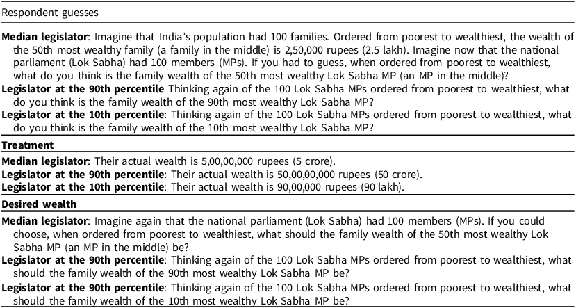
The other experimental arm entails an informational treatment, which was included in all surveys except the US YouGov survey (due to space constraints). All respondents were first given information on the wealth of the median household in their country, and were then asked to guess the wealth of a member of the national legislature at the tenth, fiftieth, and ninetieth percentiles of the legislature’s wealth distribution. After inputting the guesses, half of the respondents were randomly assigned to receive information about the actual wealth of such legislators; the other half was not shown any additional information. Subsequently, all respondents were asked to indicate their desired level of wealth of members of the national legislature at the tenth, fiftieth, and ninetieth percentiles of the legislature’s wealth distribution.Footnote 19 Table 1 gives the wording of these items in the survey in India. The wording in the other surveys was comparable, with appropriate changes to the relevant wealth values.
Informational experiment battery

The order of the two experimental arms was randomized with equal probability in each survey. In SA Section A4, we show the results of balance tests indicating that the randomizations were successfully implemented, both across and within the experimental arms. There, we also show the results of diagnostic tests indicating no effects in the conjoint experiment with respect to the order of attributes, tasks, or profiles.
Analysis and Estimation
To analyze the conjoint experiments, we follow Hainmueller et al. (Reference Hainmueller, Hopkins and Yamamoto2014) in estimating the average marginal component effects (AMCE) of candidate attributes on the outcomes outlined above. AMCE is the effect of a change in the value of an attribute, averaged over the joint distribution of all other attributes and across all respondents. Our main interest is in the AMCE of a candidate’s wealth, which measures the ceteris paribus change in a respondent’s response to an outcome question when the respondent is shown a candidate profile with that level of wealth compared to the same profile with another value of wealth, both relative to another randomly generated profile. Based on Hainmueller et al. (Reference Hainmueller, Hopkins and Yamamoto2014), we estimate the AMCEs with an OLS model of the following form:
 $$ Y_{i,t,p} = \mu + \sum _j \beta _j \;{\rm Wealth}_{i,j,t,p} + \sum _k \sum _l \beta _{kl} \;{\rm Other\ treatments}_{i,k,l,t,p} + \sum _n \gamma _n {\bf X}_{i,n} + \delta _c + \epsilon _{i,t,p}, $$
for respondent i’s response to outcome question Y after the rating task t and candidate profile p, where Wealth contains j − 1 wealth attribute values, and Other treatments
kl
contains k other candidate attributes with l − 1 values for each attribute (see SA Table A1). For four attributes (gender, party religion, and race), we code a variable indicating the shared characteristic between a candidate profile and a respondent (with respondent characteristics measured in the same way as the candidate attributes), so that the AMCEs have a more intuitive interpretation and a more natural baseline category. δ
c
are country sample indicator variables, ${\bf X}$
includes an indicator variable for the order of the two experimental arms, and whether the respondent received the informational treatment in the information experiment. Following Hainmueller et al. (Reference Hainmueller, Hopkins and Yamamoto2014), we treat each hypothetical candidate as a unique case; since multiple paired profiles are evaluated by the same respondent, we cluster the standard errors by respondent.
${\bf X}$
includes an indicator variable for the order of the two experimental arms, and whether the respondent received the informational treatment in the information experiment. Following Hainmueller et al. (Reference Hainmueller, Hopkins and Yamamoto2014), we treat each hypothetical candidate as a unique case; since multiple paired profiles are evaluated by the same respondent, we cluster the standard errors by respondent.
For hypotheses H1, H1a, H2, and H3b, outcome Y is a respondent’s candidate preference. This variable resembles vote choice, and we therefore interpret the AMCEs as the effect of a candidate’s attribute on their vote share in a hypothetical election characterized by the distribution of attributes provided in the experiment (Bansak et al. Reference Bansak, Hainmueller, Hopkins and Yamamoto2022).Footnote 20 For hypotheses H1b and H1c, the outcomes are the candidate preference and the perceived candidate effectiveness in enacting new legislation in Congress. For H1d, it is the perceived likelihood of a candidate being influenced by lobby groups.
For H1a, we augment our main specification by adding a variable capturing respondent income or wealth, as well as all the pairwise interactions with the candidate wealth variables.Footnote 21 For the second part of hypothesis H1b, we add an indicator variable of whether the respondents in the US YouGov survey were shown the candidate profiles with all the attributes, or profiles without a candidate’s occupation and education, as well as the pairwise interactions with the candidate wealth variables. To test hypothesis H2, we add the interaction terms between a candidate’s wealth and their in-group status with respect to partisan affiliation, race/ethnicity, and religion. To test hypothesis H3b, we add a double interaction between the candidate’s wealth, the variable indicating whether a respondent received the information treatment in the information experiment, and the variable capturing the accuracy of that respondent’s average guess of the national legislators’ actual wealth, as defined below. The specification also includes all the single interaction and constituent terms. This analysis is confined to the subsample in which the information experiment was ordered first, and the conjoint experiment second (half of the overall sample).
To analyze the information experiment, we compare the respondents’ guesses and their desired levels of the wealth of national legislators at the tenth, fiftieth, and ninetieth percentiles of the legislature’s wealth distribution to the actual wealth values for such legislators. All the values are on the same scale (continuous, in monetary units). For hypothesis H1, we compare the respondents’ desired levels of legislators’ wealth to the legislators’ actual levels of wealth after the respondents have received the information about the latter (in the treatment group of the information experiment). In the text, we make this comparison graphically and descriptively, with the results of formal statistical tests shown in the Supplementary Appendix. For hypothesis H3a, we do the same graphical and formal analyses, but we compare the respondents’ pre-treatment guesses of legislators’ wealth to the legislators’ actual wealth.
Finally, for hypothesis H3b, we calculate the accuracy of a respondent’s pre-treatment guess of the wealth of national legislators in the three scenarios (at the tenth, fiftieth, and ninetieth percentile of the legislature’s wealth distribution), by taking the difference for each scenario between the guess and the legislator’s actual wealth. We then take the average across the three scenarios – and divide the resulting average difference into quartiles of accuracy within each country sample – so that the lowest quartile represents the largest underestimates.
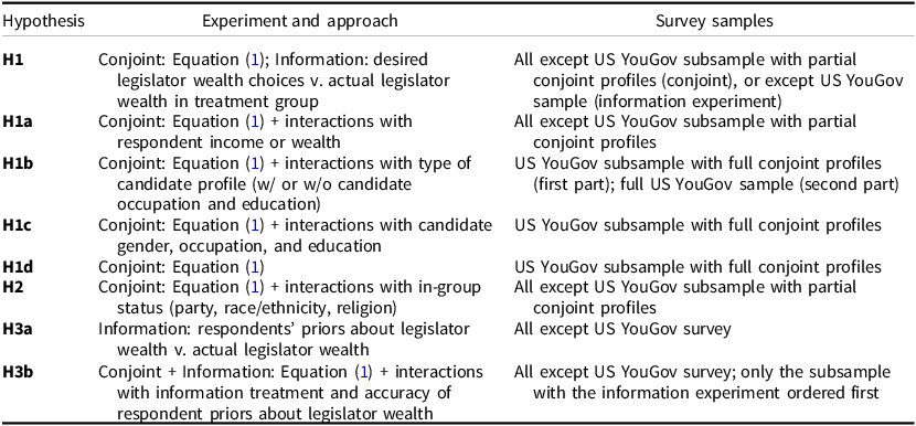
When analyzing the conjoint experiments to test hypotheses H1, H1a, H2, and H3b, we use the surveys in all four countries, with the exception of the subsample in the US YouGov survey in which the respondents were shown profiles without the candidate’s occupation and education. To test hypotheses H1b–H1d, we use either the full sample or the subsample of the US YouGov survey where the respondents were shown the full candidate profiles. When analyzing the information experiment (for hypotheses H1, H3a, and H3b), we use all the country surveys except the US YouGov survey, where the informational experiment was not included due to space constraints. We summarize the experiments, surveys, samples, and analytical approaches used to test each hypothesis in Table 2.
Analysis plan summary

Results
Does the Public Prefer Wealthier Politicians?
We begin by analyzing the conjoint experiments and estimating the AMCEs of the hypothetical candidates’ wealth. To simplify the presentation of results, we group the nine candidate wealth categories (one for each wealth decile) into five quintiles: candidate profiles with wealth at the tenth and twentieth percentile are grouped into the bottom quintile, and so on, with the profiles at the ninetieth percentile being in the top quintile. If the public directly prefers wealthier candidates, as outlined in hypothesis H1, the wealth AMCEs should be larger (and positive) for higher quintiles compared to lower quintiles.
The top part of Figure 2 displays the wealth AMCEs, with the bottom quintile as the baseline category. Contrary to H1, the public in our four countries on average shows a clear preference against, rather than for, wealthier hypothetical candidates. For example, compared to candidates in the bottom quintile of wealth, the vote share of the hypothetical candidates in the top quintile is lower by 10.5 percentage points (statistically significant at p < 0.01). Also, the level of a candidate’s wealth clearly mattered to the respondents. For example, the drop in support for a candidate in the top quintile was more than double that for a candidate in the third quintile ( − 10.5 percentage points vs. − 5 percentage points; the difference is significant at p < 0.01), roughly the same difference as between the third and first quintile. While there is some variation in its magnitude, the predisposition against wealthier candidates is present in all four countries (SA Figure A3).
Candidate attribute effects on candidate preference.

Aside from wealth, several other attributes show statistically significant effects on candidate preference.Footnote 22 The public strongly prefer co-partisan candidates, and those with the same religious affiliation as their own; however, we see less strong and less consistent in-group preferences by gender or race/ethnicity (though we observe significant effects of co-ethnicity in Chile and India; see SA Figure A3). Respondents are by and large less supportive of candidates with higher-earning occupations (relative to the baseline occupation of teacher), though less consistently than in terms of candidate wealth. They are also less supportive of candidates with prior experience in local legislatures (compared to teachers) in three of the four countries. The effects of educational attainment or prestige are somewhat mixed, with respondents in the United States being less supportive and respondents in other countries more supportive of candidates with more education/educational prestige.
Another way for us to assess public preferences towards candidate wealth is to analyze the information experiment, by comparing the respondents’ desired wealth of their national legislators to the legislators’ actual wealth. We do so in the treatment group, after the respondents have been informed of the legislators’ true wealth. According to H1, the legislators’ wealth desired by the public should be no lower, and potentially higher, than the true level of legislators’ wealth. If, on the other hand, the public prefers a less wealthy political class, as suggested by the conjoint results, the respondents’ desired wealth of legislators should be lower than their revealed actual wealth. Consistent with the conjoint results, and not with our hypothesis, Figure 3 shows that the majority of respondents would prefer a less wealthy political class (although there is wide variation in preferences, as indicated by the horizontal axis, expressed on a logarithmic scale). This is the case when asked about the wealth of a legislator at the median of the legislature’s wealth distribution, and especially at the ninetieth percentile, as the responses (gray bars) generally cluster below the actual legislator wealth (vertical black lines; these differences are significant at p < 0.01 based on one-sample t-tests; see SA Table A8). We observe similar patterns in each country (SA Figure A4).
Respondents’ preferred v. actual wealth of national legislators.

Wealth as aspiration
Despite the patterns in Figures 2 and 3, we proceed to evaluate whether there is evidence, at least at the margin, for a direct preference in favor of wealthier candidates. We first assess evidence with respect to public aspirations, by evaluating whether support for wealthier candidates may be stronger among respondents with lower income or wealth, as indicated in hypothesis H1a.
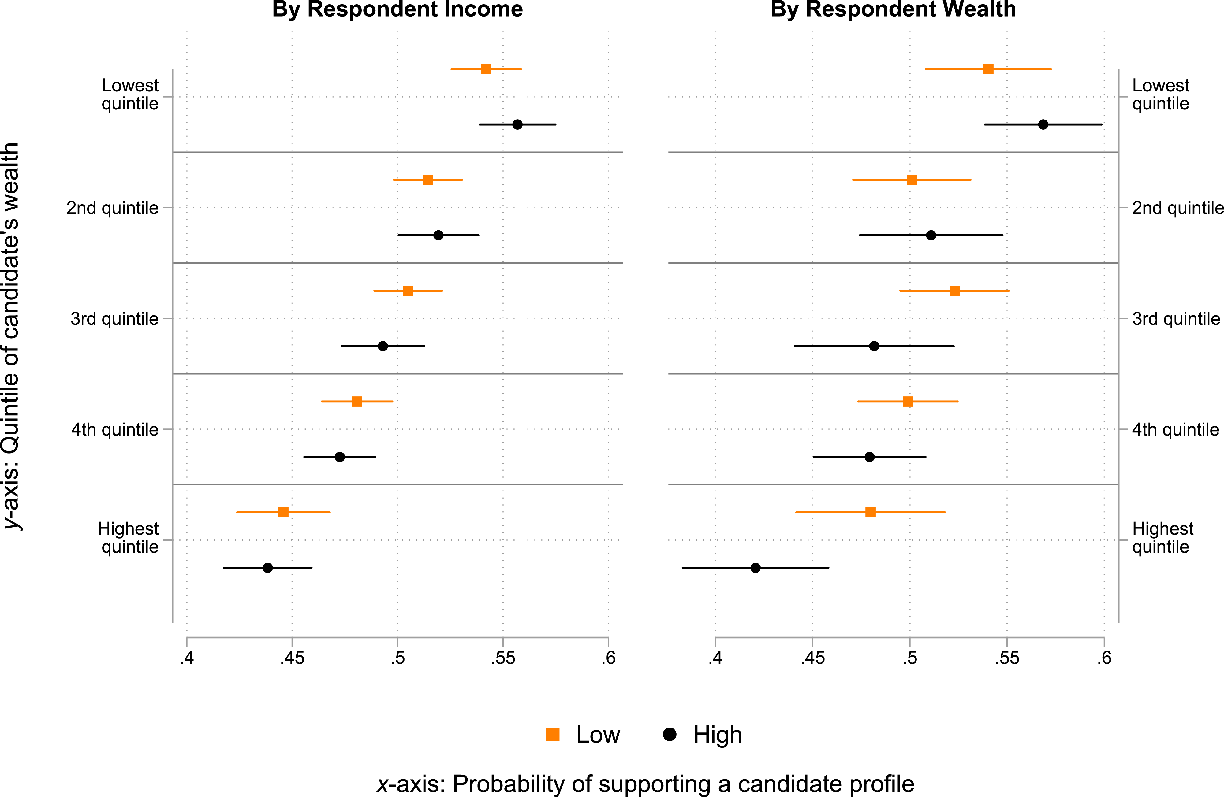
Figure 4 shows the average predicted vote share (or marginal means; Leeper et al. Reference Leeper, Hobolt and Tilley2020) in the conjoint experiment for candidates in each wealth sextile, by respondent income (left panel) and wealth (right panel). Estimates in orange squares are for respondents with lower income or wealth, and in black circles for respondents with higher income or wealth. The left panel shows that the decreasing preference for wealthier candidate profiles that we saw in Figure 2 varies little by respondent income, as the patterns among higher-income respondents are nearly indistinguishable and not statistically different from the patterns among lower-income respondents. We see somewhat larger differences by respondent wealth in a manner more consistent with H1a. The less wealthy respondents, who presumably harbor greater aspirations for higher social status than wealthier respondents, tend to be somewhat more supportive of wealthier politicians.Footnote 23 For example, the predicted support for hypothetical candidates with wealth in the highest quintile is on average about 6 percentage points higher among the less wealthy than the wealthier respondents (significant at p < 0.05). That said, this greater preference for wealthier candidates is only relative, as we still see a negative ‘gradient’ among both groups of respondents, albeit of lower magnitude among the less wealthy respondents.Footnote 24 Therefore, these patterns are insufficient to conclude that differences in aspirations may plausibly drive public support for wealthier candidates.
Respondent income or wealth and preference for wealthy candidates.

Wealth as proxy for other qualities
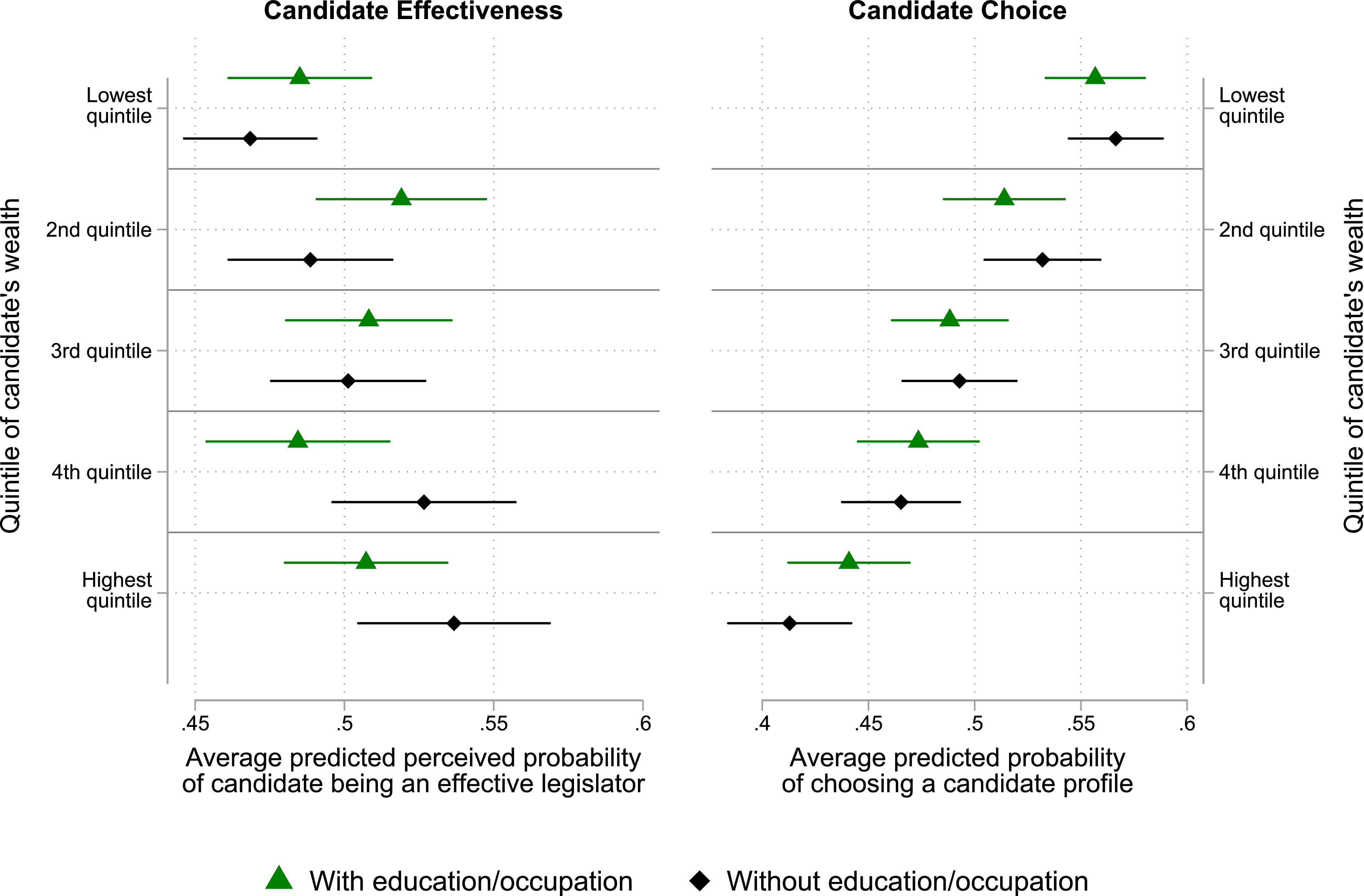
Next, we test hypothesis H1b – whether the support for wealthier candidates may be driven by wealth acting as a proxy for other desirable qualifications such as skill or effectiveness. To assess this possibility, we examine the effect of wealth and other candidate attributes on the respondents’ perceptions of a candidate’s effectiveness in enacting new legislation in the legislature. As mentioned above, we focus on the sample of US respondents in the YouGov survey, where we asked this outcome question.
Candidate attribute effects on perceived effectiveness as legislators.

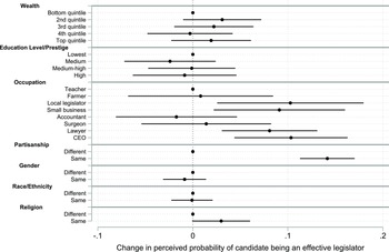
Figure 5 shows no evidence that respondents perceive wealthier candidates as potentially more effective legislators, which is inconsistent with the first part of H1b. The respondents also did not use the prestige of a candidate’s education to infer their potential effectiveness. However, there is clear evidence that the candidate’s occupation served as an informative signal. Hypothetical candidates with prior political experience, lawyers, and executives (small business owners and CEOs) were perceived as significantly more likely to be effective than other candidate profiles, including the high-earning white-collar professions of surgeons and accountants. For example, the average predicted probability of being an effective legislator for CEOs is 12.1 and 9.1 percentage points greater than for accountants and surgeons, respectively (both differences significant at p < 0.01).
This evidence raises the question, posed in the second part of H1b, as to whether respondents may be more likely to use wealth to infer such qualifications in the absence of information on occupation and education. The left panel of Figure 6 shows evidence consistent with this expectation. For example, when respondents saw a candidate’s education and occupation as well as their wealth, they were no more likely to expect a candidate in the fourth or top quintile of wealth to be an effective legislator than a bottom-quintile candidate (difference of 1 percentage point, p = 0.57). However, when information on occupation and education was omitted, the wealthier candidates were on average 6.3 percentage points (p < 0.01), or about 14 per cent, more likely to be seen as effective (the difference between these two trends is significant at p < 0.05). To a degree, therefore, wealth does seem to serve as a proxy for qualities that the public desires of a political candidate.
However, the right panel of Figure 6 indicates that this inferential role of wealth does not translate into greater support for wealthier candidates: they were less preferred than the less wealthy candidates at very similar rates irrespective of whether respondents saw their full profiles or those that omitted information about education and occupation. Our data, therefore, provides no evidence that when serving as a cue for positive traits, a candidate’s wealth helps boost their electoral appeal.
Wealth as proxy for occupational or educational qualifications.

As outlined in hypothesis H1c, however, the question remains as to whether wealth of a candidate that may be considered surprising might serve as a particularly effective signal of quality or skill to such an extent as to induce a greater preference for wealthier candidates. Due to space constraints, we show the results in SA Section A5.5. In summary, we do not find consistent evidence for this possibility. The wealthiest women candidates do receive a higher vote share than the wealthiest men, but we see similar gender patterns for other wealth levels, too. Moreover, less wealthy men are still clearly preferred to wealthy women, not just wealthy men. The patterns for occupation and education are similar.Footnote 25 In addition, we find even fewer differences in terms of perceptions of a candidate’s effectiveness in enacting legislation. In sum, there is no evidence that potentially surprising wealth serves as a strong signal for effectiveness, and thus an inferential cue that drives electoral support.
Wealth as buffer against capture
Next, we evaluate hypothesis H1d, proposing that the public supports wealthy candidates because wealth is seen as a buffer against capture by special interests. If so, then our respondents should be less likely to perceive the wealthier candidates as susceptible to capture. We again focus on the US YouGov survey where we asked the relevant outcome question. Figure 7 shows the wealth and other candidate attribute AMCEs. Contrary to H1d, our respondents perceived wealthier candidate profiles as more, not less, likely to be influenced by lobby groups. For example, a candidate with wealth in the top quintile was on average seen as 11 percentage points more likely than the bottom-quintile candidate to be influenced by a lobby group (p < 0.01). It is therefore unlikely that perceptions of wealth as inoculating against special interests help engender a direct public preference for wealthier politicians.
Candidate attribute effects on perceived influence by lobby groups.

Do In-Group Biases Produce Indirect Preferences for the Wealthy?
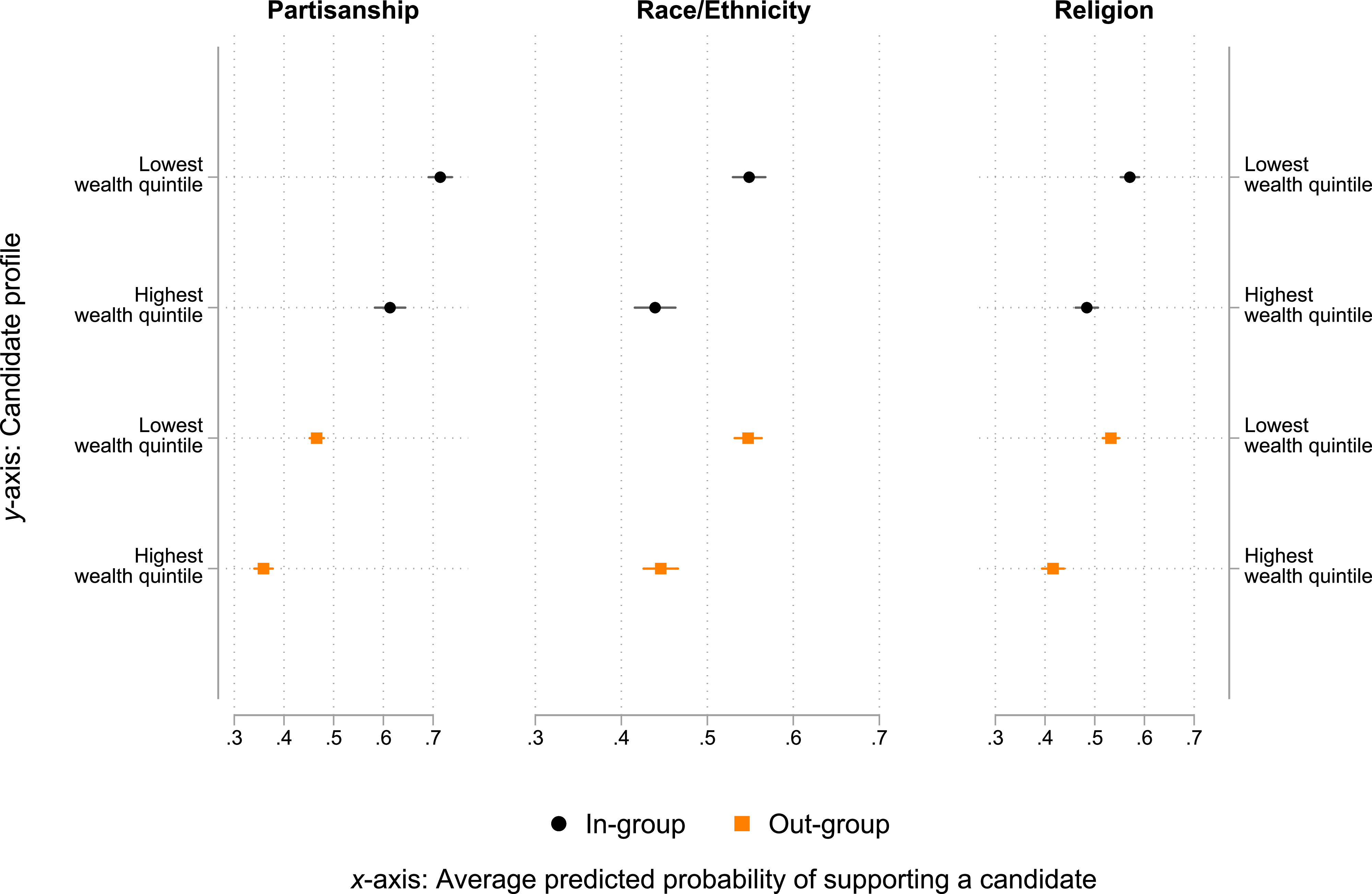
In sum, our data offers scant evidence that the public in the countries we surveyed directly prefer wealthier politicians. Is there evidence for indirect or even inadvertent support for the wealthy? Hypothesis H2 states that the public may exhibit in-group biases such that the in-group wealthy candidates are preferred to the out-group non-wealthy candidates even in the absence of a direct preference for greater candidate wealth. To evaluate this possibility, we examine the strength of in-group preferences and how they interact with preferences over candidate wealth for the three widely studied group attachments included in our conjoint profiles: partisan affiliation, race/ethnicity, and religion. As mentioned above, an in-group candidate is one who shares a characteristic with the respondent: affiliation with a respondent’s preferred political party, the same race, ethnicity, caste, or religion. To test H2, Figure 8 compares the average predicted vote shares of the in-group (black circles) and out-group (orange squares) wealthy candidates (with wealth in the top quintile) and less wealthy candidates (with wealth in the bottom quintile), for partisan affiliation in the left panel, race/ethnicity/caste in the middle panel, and religion in the right panel.
In-group biases and preference for wealthy candidates.

Consistent with the results in the previous section, each panel in the figure shows that a bottom-quintile candidate is preferred to a top-quintile candidate, for both the in-group and out-group profiles. Perhaps unsurprisingly, the co-partisan and co-religious bottom-quintile candidates tend to receive the highest support (for race/ethnicity/caste, the in-group and out-group bottom-quintile candidates receive very similar vote shares). Most relevant for the expectations in H2, however, is the comparison between the vote share for the in-group wealthier candidate profile (the second-top estimate in each panel) and the out-group less wealthy candidate profile (the second-from-bottom estimate in each panel). As can be seen in the left panel of Figure 8, consistent with H2, respondents were 12.2 percentage points more likely to support a co-partisan wealthy candidate than a less wealthy candidate from another party (p < 0.01). That is, a candidate’s party affiliation trumps their wealth, even though respondents clearly and strongly prefer candidates of lower wealth. In other words, we see evidence of partisan bias inducing an indirect preference for wealth. This is not surprising given the patterns we observed in Figure 2, where the effects of the co-partisan AMCE were by far the strongest in magnitude.Footnote 26 It is likely that we do not see similar patterns for the other two group attachments – race/ethnicity/caste and religion – because these in-group preferences in the conjoint experiment were not strong enough to override the preference against wealthier candidates.
The results for partisan attachments therefore suggest the possibility that wealthy politicians may benefit from in-group biases. At the same time, we note that in the countries we examine, partisan bias can at best be a partial explanation for the prevalence of wealthy political elites. Namely, the rates of partisan attachments vary widely across the four countries. The share of respondents in our data who report identifying with a party ranges from the lows of 10 per cent in Brazil and 19 per cent in Chile, to 33 per cent in India and more than 60 per cent in the United States. Even with strong partisan bias, such low shares of partisans in Brazil and Chile (consistent with arguments made elsewhere; see, for example, Mainwaring Reference Mainwaring2018) can hardly account for all of the electoral advantage enjoyed by the wealthy.
Does Ignorance Produce Inadvertent Preference for the Wealthy?
The necessary condition for voters to prefer – or disprefer – candidates of certain wealth is that they are aware of it. If voters misperceive how wealthy the political elites are, they might overlook a factor that may otherwise have electorally disadvantaged the wealthier candidates. In other words, the political class may be wealthy because of the lack of voter awareness. As outlined in hypothesis H3, for public ignorance to inadvertently advantage the wealthy it must be that: (a) respondents generally underestimate the wealth in the political class, and (b) correcting such misperceptions would lead to lower support for wealthier candidates.
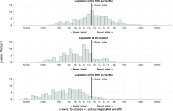
To determine the degree to which the public is aware of how wealthy the political elites are, we turn back to our informational experimental arm, where we asked respondents to guess the wealth of national legislators at the tenth, fiftieth, and ninetieth percentiles of the legislature’s wealth distribution (see Table 1). In Figure 9, we show descriptively how those guesses compare to the actual wealth of such legislators (shown as horizontal lines in each panel). While some respondents underestimate the wealth of legislators at the tenth percentile, the distribution of guesses is centered almost exactly at zero. This means that the majority of respondents lodge quite accurate guesses for this scenario (even though the horizontal axis shows wide variation in the precision of the respondents’ guesses). However, they considerably underestimate the wealth of legislators at the median and especially the ninetieth percentile (which is confirmed formally by the one-sample t-tests in SA Table A8). These patterns indicate that indeed, as posited by H3a, the public’s priors about the wealth of political elites are quite inaccurate.
Respondents’ guesses vs. actual wealth of national legislators.

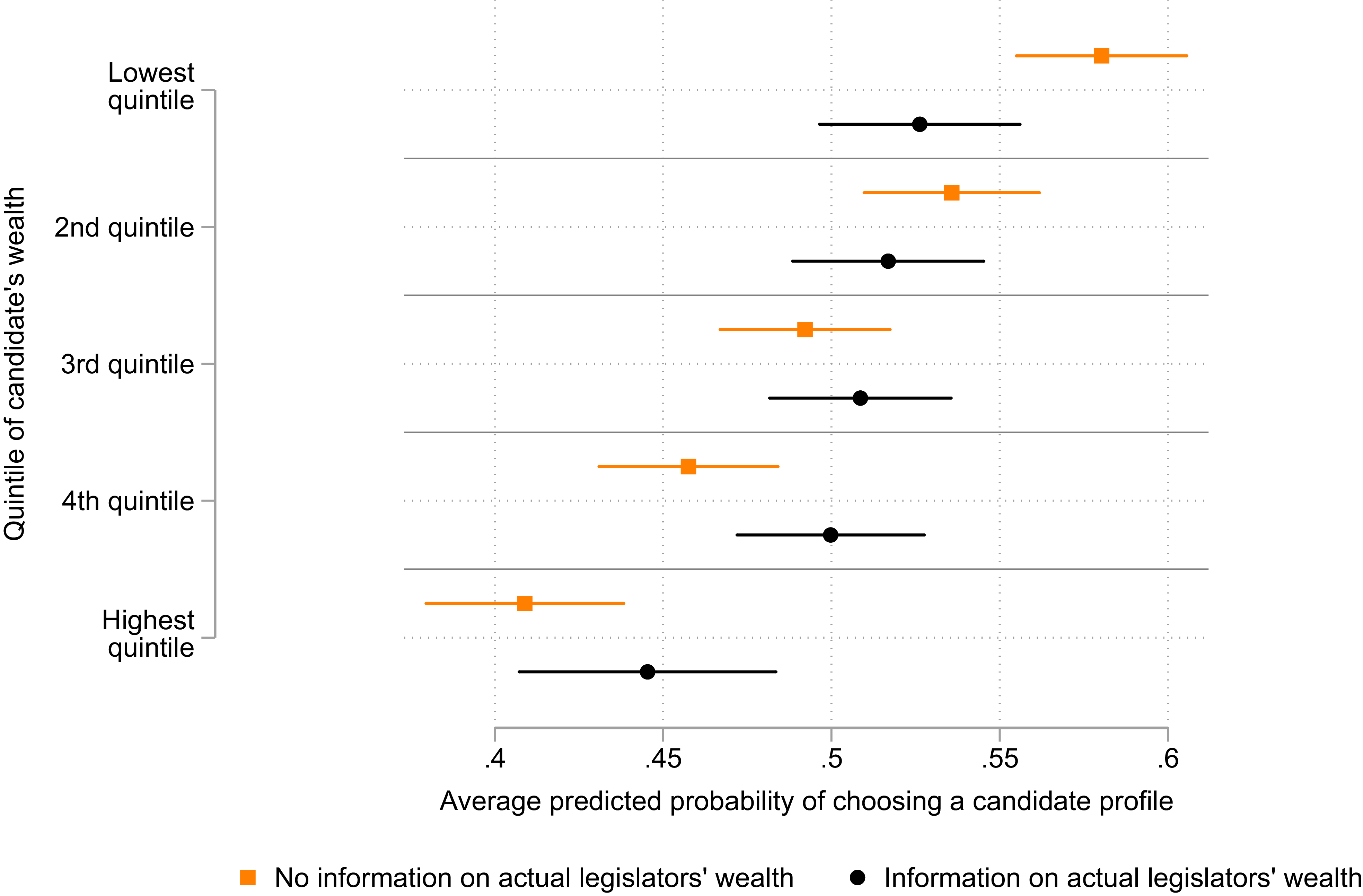
Are such misperceptions consequential for the extent of support of wealthier compared to the less wealthy candidates? If so, then according to hypothesis H3b, providing information about the true wealth of the political class should reduce the support for wealthier candidates. We test that proposition by combining the conjoint and informational experiments. Figure 10 plots the predicted average vote share for candidate profiles in each wealth quintile, separately for respondents who were not exposed to the informational treatment (orange squares) and those who were (black circles).Footnote 27 Hypothesis H3b predicts that the average vote share of the wealthier candidate profiles should be lower (relative to the less wealthy candidate profiles) among the latter group of respondents. Figure 10, however, shows the opposite pattern. While both groups of respondents prefer the less wealthy to the wealthier candidate profiles, this tendency is more pronounced among the respondents who did not receive the informational treatment. For example, the average vote share of a top-quintile candidate among respondents not treated with information is 17.1 percentage points lower than the vote share of a bottom-quintile candidate (p < 0.01). The same quantity among the treated respondents is less than half that: 8.1 percentage points (p < 0.01; the difference between the two is also significant at p < 0.01).
Information about legislators’ wealth and preference for the wealthy.

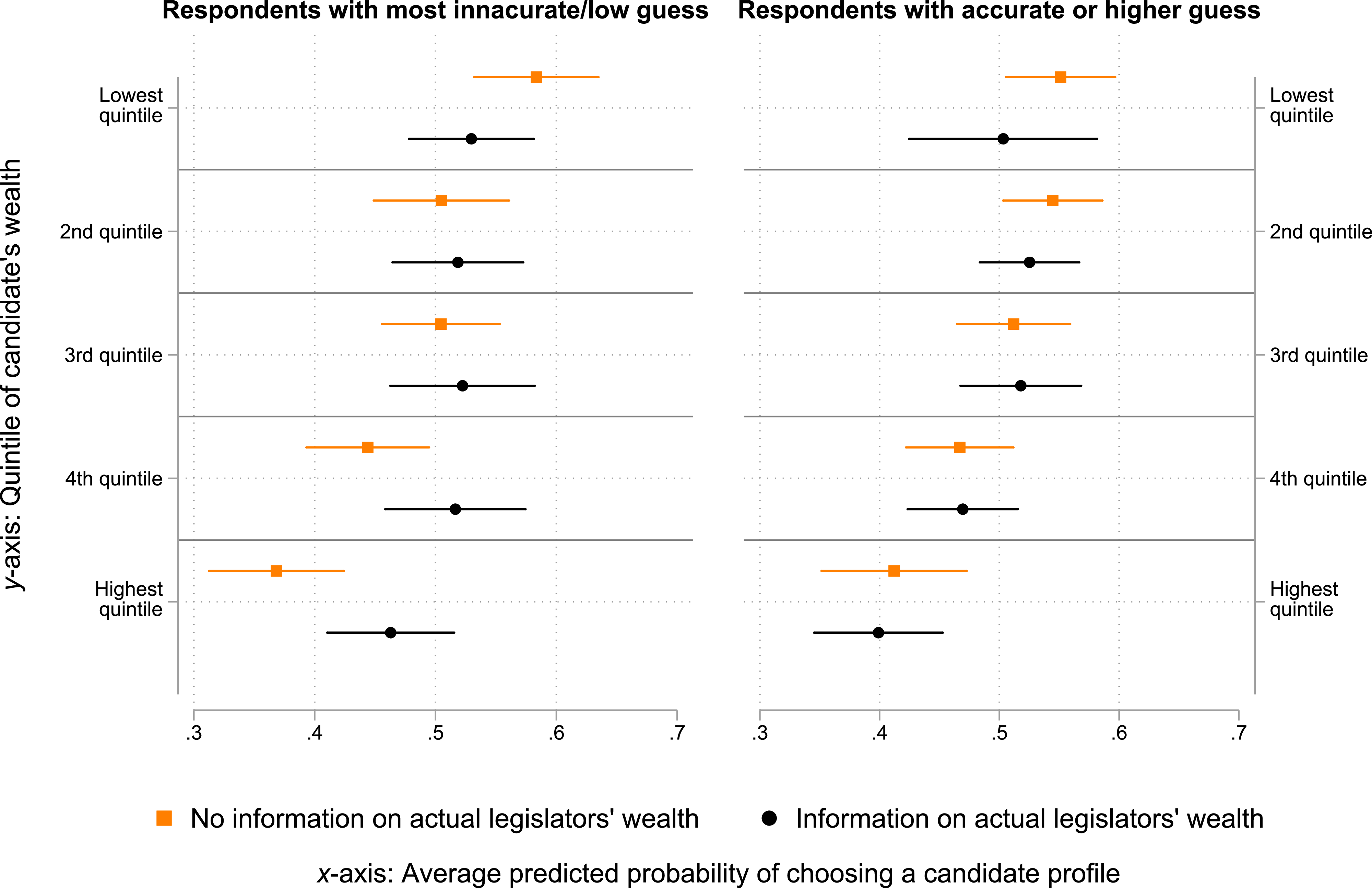
While this pattern is seemingly inconsistent with H3b, it could be that it is driven by the respondents with more accurate priors, whereas respondents with less accurate priors reacted to information in line with the expectations in H3b. To check that, Figure 11 shows the same results as in Figure 10, but separately in the left panel for the respondents with inaccurate priors (the quartile of respondents with the largest underestimate of the legislators’ true wealth), and in the right panel for the respondents with accurate priors (the quartile of respondents with the smallest underestimate or slight overestimate of the legislators’ true wealth).Footnote 28
Information about legislators’ wealth and preference for the wealthy, by accuracy of respondent guesses of legislators’ wealth.

The figure reveals that the informational treatment fails to produce the anticipated effect precisely for the group that was expected to be the most likely beneficiary of information. That is, it is the respondents with the least accurate priors who are less inclined to reduce the support for wealthier candidates in response to the information treatment. For example, among these respondents, the average vote share for the highest-quintile candidate is 9.5 percentage points higher when they receive the treatment than when they do not (p < 0.02); for those with more accurate priors, there is essentially no difference ( −1 percentage points, p = 0.8; the difference between the two estimates is significant at p < 0.07). In SA Section A5, we show that a plausible reason for this is that the information treatment seems to have normalized the unexpectedly large wealth of national legislators among the respondents with inaccurate priors.Footnote 29 In response to the informational treatment, these respondents increased their post-treatment desired levels of legislators’ wealth compared to their pre-treatment guesses, whereas we observe no such change among the respondents with more accurate priors.
In sum, while the public considerably underestimates the wealth of the political class, correcting such misperceptions does not (additionally) reduce the support for wealthier candidates. If anything, the informational treatment achieves the opposite result, somewhat increasing (in relative terms) the support for wealthier candidates among the less informed parts of the public. Our data therefore suggests that it is unlikely that the over-representation of wealth in politics owes to public misperceptions of candidate wealth, even though they are quite common.
Conclusion
Our paper asked whether the over-representation of the wealthy in politics reflects the preferences of the public. Utilizing two experiments from five original surveys fielded in four countries, our evidence indicates that the answer is very likely no. At best, wealth serves as a mixed signal. It potentially activates social-status aspirations, but only among a limited subset of respondents. It raises somewhat the expectations about a candidate’s effectiveness in politics, but also about their proclivity to cater to special interests (and to use money to buy votes). Wealthy politicians may benefit from voters caring more about group affiliation than wealth. However, while we find some evidence of such in-group bias with respect to partisan attachments, we do not find it for other prominent group markers such as race, ethnicity, and religion. Finally, the public grossly underestimate the wealth of the political class. Nonetheless, when corrected, such misperceptions do not noticeably change the already low support for wealthier candidates.
The over-representation of wealth in politics therefore likely owes primarily to other, supply-side driven factors. With deeper pockets and stronger connections to donors, wealthier candidates are better positioned to defray high costs of campaigning (Avis et al. Reference Avis, Ferraz, Finan and Varjão2022; Motolinia et al. Reference Motolinia, Klašnja and Weschle2025). This may be especially true of candidates who have traditionally faced greater barriers to entry (such as women; Bernhard et al. Reference Bernhard, Eggers and Klašnja2023). Perhaps as a consequence, party elites may prefer such candidates, who can self-finance, spread the wealth, and bring in other well-heeled donors (Carnes Reference Carnes2020).
That said, our results do not preclude the possibility that a candidate’s wealth does produce some advantages with voters. Perhaps most plausibly, wealthier candidates, especially non-incumbents, may use their resources to build greater name recognition, signaling higher viability (Kam and Zechmeister Reference Kam and Zechmeister2013; Larreguy, Marshall and Snyder Reference Larreguy, John and Snyder2018). Yet, our results would suggest that such dividends to candidate wealth do not stem from the voters’ valuation of wealth per se, or of their ignorance, but from its instrumental value in achieving recognition or other precious political commodities. We believe that these conjectures are fruitful directions for future research. In addition, future work should examine more closely how surprising wealth shapes voter perceptions, as it may signal ability, inherited advantage, or even potential corruption. Distinguishing between these possibilities would deepen our understanding of the link between wealth and political appeal.
Supplementary material
Supplementary material for this article can be found at https://doi.org/10.1017/S0007123425100938.
Data availability statement
Replication data for this article can be found in Harvard Dataverse at: https://doi.org/10.7910/DVN/1KQCDN.
Acknowledgements
For helpful comments and suggestions, we thank Simón Ballesteros, Taylor Carlson, Nick Carnes, Maria Carreri, Simon Chauchard, William Franko, Brian Hamel, Anna Paula Pellegrino, Daniel Smith, Hye Young You, Simon Weschle, Amber Wichowsky, and participants at the 2024 APSA meetings, 2024 MPSA meetings, 2024 Copenhagen Money in Politics Conference, 2024 Toronto/Montreal Political Behavior Workshop, 2025 Rebecca B. Morton Conference on Experimental Political Science, 2025 Political Economy of Representation Workshop, and at seminars at Georgetown University and Washington University in St Louis. We thank Parushya Parushya, Leticia Claro, and Raduan van Velthem Meira for excellent research assistance, and the teams at The American Social Survey (TASS) and the Weidenbaum Center Survey (WCS) for their support.
Financial support
This project was financially supported by the Weidenbaum Center at the Washington University in St. Louis (WUSTL) and was partially implemented through The American Social Survey (TASS) and the Weidenbaum Center Survey (WCS).
Competing interests
The authors declare none.


 Open access