Nomenclature

AI

artificial intelligence

ANN

artificial neural network

CART

classification and regression trees

CNN

convolutional neural network

DL

deep learning

GRU

gated recurrent unit

LR

linear regression

LSTM

long short-term memory

MAE

mean absolute error

ML

machine learning

MLP

multilayer perceptron

MSE

mean square error

QAR

quick access recorder

ReLU

rectified linear unit

RF

random forest

RMSE

root mean square error

SVM

support vector machine

SVR

support vector regression

TF

TensorFlow

TFLite

TensorFlow Lite

UAV

unmanned aerial vehicle

XGBoost

extreme gradient boosting

${V_1}$

decision speed

${V_R}$

rotation speed

${V_2}$

takeoff safety speed

2.0 Deep learning

Deep learning denotes the family of machine learning techniques in which multi-layer artificial neural networks are trained end-to-end to extract hierarchical patterns directly from raw data [Reference LeCun, Bengio and Hinton27, Reference Goodfellow, Bengio and Courville28]. The defining departure from classical machine learning lies in the representation step: whereas conventional pipelines rely on hand-crafted predictors that are fed unchanged to the regressor, a deep network discovers its own intermediate representations during training. This data-driven feature extraction has made deep learning the dominant approach in domains as diverse as computer vision, speech recognition, time-series forecasting and flight-parameter estimation in aviation.

In this study, four deep learning architectures were selected for takeoff speed prediction. These architectures are MLP, 1D-CNN, LSTM and a wide-and-deep architecture with multi-head self-attention. The selected architectures are briefly explained below.

2.1 Multilayer perceptron

The MLP is the basic and most widely used fully connected feed-forward neural network. The MLP consists of an input layer, one or more hidden layers and an output layer. In each layer, the inputs are multiplied with the weights and the bias term is added. Then, a nonlinear activation function is applied to obtain the output of the layer. The mathematical model of a hidden layer of the MLP is given in Equation (1).

(1) \begin{align}{{\bf{h}}_\ell } = \sigma({{{\bf{W}}_\ell }{{\bf{h}}_{\ell - 1}} + {{\bf{b}}_\ell }}),{\rm{\;\;\;\;}}{{\bf{h}}_0} = {\bf{x}}, \end{align}

Here, ${{\bf{h}}_\ell }$ is the output of the $\ell $ -th layer, ${{\bf{W}}_\ell }$ is the weight matrix, ${{\bf{b}}_\ell }$ is the bias vector, ${\bf{x}}$ is the input vector and $\sigma (\!\cdot\!)$ is the nonlinear activation function. In this study, the rectified linear unit (ReLU) is selected as the activation function. The final layer is a linear layer and produces the scalar takeoff speed estimate. To prevent overlearning, dropout [Reference Srivastava, Hinton, Krizhevsky, Sutskever and Salakhutdinov29] and ${L_2}$ weight decay are used in the hidden layers. The MLP is the basic deep learning model and is used as a reference point for comparison with other deep learning architectures.

2.2 One-dimensional convolutional neural network

The 1D-CNN is a deep learning architecture that applies the convolution operation along a single dimension [Reference LeCun and Bengio30]. In this study, the four input features are reshaped into a short signal of length $T = 4$ with a single channel, and the convolution layers are applied along this length dimension. The output of a one-dimensional convolution layer is given in Equation (2).

(2) \begin{align}{y_{c,t}} = \sigma\! \left( {\mathop \sum \limits_{c{\rm{'}} = 1}^{{C_{{\rm{in}}}}} \mathop \sum \limits_{\tau = 0}^{k - 1} {w_{c,c{\rm{'}},\tau }}{\rm{\;}}{x_{c{\rm{'}},t + \tau }} + {b_c}} \right)\!, \end{align}

Here, ${y_{c,t}}$ is the output of the convolution operation at the position $t$ for the output channel $c$ , ${w_{c,c{\rm{'}},\tau }}$ are the weights of the convolution kernel of size $k$ , ${b_c}$ is the bias term and $\sigma (\!\cdot\!)$ is the ReLU activation function. After a stack of convolution layers, a global average pooling layer is used to aggregate the temporal axis, and a dense head produces the takeoff speed estimate. The 1D-CNN was selected to investigate whether the parameter sharing across the four predictors provides any benefit on this tabular data set.

2.3 Long short-term memory

The LSTM, introduced by Hochreiter and Schmidhuber [Reference Hochreiter and Schmidhuber31], is one of the most widely used recurrent neural networks in aviation deep learning applications [Reference Kang, Shang, Feng, Zheng, Liu, Qiang and Wei9, Reference Kovarik, Doherty, Korah, Mulligan, Rasool, Mehta, Bhavsar and Paglione17, Reference Jarry, Delahaye and Feron18]. The LSTM cell contains a cell state, a hidden state and three gates, namely the input gate, the forget gate and the output gate. These gates control the information flow in the cell state and allow the network to capture long-term dependencies between the input sequence elements. The mathematical model of an LSTM cell is given in Equation (8).

(3) \begin{align} {{\bf{f}}_t} &= {\sigma _g}( {{{\bf{W}}_f}{{\bf{x}}_t} + {{\bf{U}}_f}{{\bf{h}}_{t - 1}} + {{\bf{b}}_f}}\!), \\[-8pt] \nonumber \end{align}

(4) \begin{align} {{\bf{i}}_t} &= {\sigma _g}( {{{\bf{W}}_i}{{\bf{x}}_t} + {{\bf{U}}_i}{{\bf{h}}_{t - 1}} + {{\bf{b}}_i}} ),\\[-8pt] \nonumber \end{align}

(5) \begin{align} {{\bf{o}}_t} &= {\sigma _{g}}( {{{\bf{W}}_o}{{\bf{x}}_t} + {{\bf{U}}_o}{{\bf{h}}_{t - 1}} + {{\bf{b}}_o}} ), \\[-8pt] \nonumber\end{align}

(6) \begin{align} {{\tilde{\bf c}}_t} &= {\rm{tanh}}( {{{\bf{W}}_c}{{\bf{x}}_t} + {{\bf{U}}_c}{{\bf{h}}_{t - 1}} + {{\bf{b}}_c}} ),\\[-8pt] \nonumber \end{align}

(7) \begin{align} {{\bf{c}}_t} &= {{\bf{f}}_t} \odot {{\bf{c}}_{t - 1}} + {{\bf{i}}_t} \odot {{\tilde{\bf c}}_t}, \\[-8pt] \nonumber \end{align}

(8) \begin{align} {{\bf{h}}_t} &= {{\bf{o}}_t} \odot {\rm{tanh}}( {{{\bf{c}}_t}} ), \\[10pt] \nonumber \end{align}

Here, ${{\bf{x}}_t}$ is the input vector at time step $t$ , ${{\bf{h}}_t}$ is the hidden state, ${{\bf{c}}_t}$ is the cell state, ${{\bf{f}}_t}$ , ${{\bf{i}}_t}$ and ${{\bf{o}}_t}$ are the forget, input and output gates, respectively, ${{\bf{W}}_{\rm{*}}}$ and ${{\bf{U}}_{\rm{*}}}$ are the weight matrices, ${{\bf{b}}_{\rm{*}}}$ are the bias vectors, ${\sigma _g}(\!\cdot\!)$ is the logistic activation function and $ \odot $ is the element-wise multiplication. In this study, the four input features were reshaped as a sequence of length four and the LSTM model was created with two stacked LSTM layers followed by a dense head to produce the takeoff speed estimate. Although the input features are not chronologically ordered, the LSTM cells can discover the nonlinear interactions between adjacent features through the recurrent gates.

2.4 Wide-and-deep architecture with self-attention

The wide-and-deep architecture combines a linear projection of the raw inputs (the wide branch) with a deeper learned representation (the deep branch), and the two branches are concatenated to produce the output [Reference Cheng, Koc, Harmsen, Shaked, Chandra, Aradhye, Anderson, Corrado, Chai and Ispir32]. In this study, a multi-head self-attention block is used in the deep branch in the style of the TabTransformer architecture [Reference Huang, Khetan, Cvitkovic and Karnin33, Reference Vaswani, Shazeer, Parmar, Uszkoreit, Jones, Gomez, Kaiser and Polosukhin34]. Each input feature is first projected to an $e$ -dimensional embedding vector. Then, the multi-head self-attention block is applied to the embedded features as given in Equation (9).

(9) \begin{align}{\rm{Attention}}({{\bf{Q}},{\bf{K}},{\bf{V}}}) = {\rm{softmax}}\!\left( {\frac{{{\bf{Q}}{{\bf{K}}^ \top }}}{{\sqrt {{d_k}} }}} \right){\bf{V}}, \end{align}

Here, ${\bf{Q}}$ , ${\bf{K}}$ and ${\bf{V}}$ are the query, key and value matrices, respectively, which are obtained by the linear projections of the embedded features, and ${d_k}$ is the dimension of the keys. Residual connections and layer normalisation are applied around the attention and feed-forward sub-layers to stabilise the training. The output of the attention block is flattened and concatenated with a 16-unit linear projection of the raw inputs (the wide branch), and the result is passed through a final dense layer to produce the takeoff speed estimate. This architecture was included in the comparison to represent the modern tabular deep learning family [Reference Huang, Khetan, Cvitkovic and Karnin33, Reference Ark and Pfister35].

2.5 Loss function and optimisation

All four deep learning models were trained by minimising the mean square error (MSE) loss function. The mathematical model of the MSE loss function is given in Equation (10).

(10) \begin{align}{{\cal L}_{{\rm{MSE}}}} = {1 \over N}\mathop \sum \limits_{i = 1}^N {({y_i} - {\hat y_i})^2}, \end{align}

Here, $N$ is the number of training samples, ${y_i}$ is the actual takeoff speed of the $i$ -th sample and ${\hat y_i}$ is the predicted takeoff speed of the $i$ -th sample. The Adam optimiser [Reference Kingma and Ba36] was used to update the weights of the network during training. To further improve the training performance, early stopping on the validation loss and a learning rate scheduler that halves the learning rate when the validation loss plateaus were applied during training. After the base model training step, Bayesian hyperparameter optimisation [Reference Shahriari, Swersky, Wang, Adams and de Freitas37] was applied to the best-performing base model with the Keras Tuner library [Reference O’Malley, Bursztein, Long, Chollet, Jin and Invernizzi38] to obtain the final tuned model.

2.6 Performance metrics

The root mean square error (RMSE) expressed in Equation (11), the MSE expressed in Equation (12) and the mean absolute error (MAE) expressed in Equation (13) were used as the performance criteria for the evaluation of the deep learning models. These metrics were also used in the previous study [Reference Karaburun, Ark Hatipoglu and Konar26] for the takeoff speed prediction problem and are widely accepted as the standard regression metrics in the literature [Reference Chicco, Warrens and Jurman39]. The smaller the error value, the higher the model accuracy is considered.

(11) \begin{align}{\rm{RMSE}} = \sqrt {{1 \over N}\mathop \sum \limits_{i = 1}^N {{({y_i} - {{\hat y}_i})}^2}}, \end{align}

(12) \begin{align} {\rm{MSE}} = {1 \over N}\mathop \sum \limits_{i = 1}^N {({y_i} - {\hat y_i})^2}, \\[-8pt] \nonumber \end{align}

(13) \begin{align} {\rm{MAE}} = {1 \over N}\mathop \sum \limits_{i = 1}^N \left| {{y_i} - {{\hat y}_i}} \right|\!. \\[10pt] \nonumber \end{align}

Here, $N$ is the number of test samples, ${y_i}$ is the actual takeoff speed of the $i$ -th test sample and ${\hat y_i}$ is the predicted takeoff speed of the $i$ -th test sample.

3.0 Problem definition

This section describes the data set, the pre-processing pipeline and the training protocol that were adopted to obtain the deep-learning takeoff-speed predictors compared in the remainder of the paper.

The training corpus is the Boeing 737-300 performance data set distributed in the manufacturer’s aircraft operations manual [6] and reused, for direct comparability, from the earlier study of Karaburun et al. [Reference Karaburun, Ark Hatipoglu and Konar26]. Five quantities are recorded for every entry: pressure altitude (ft), outside air temperature ( ${^ \circ }$ F), gross weight (klb), flap angle ( ${^ \circ }$ ) and takeoff speed (kn). The data span the operational ranges 0–9,000 ft, $\left( { - 40} \right)$ – $160{^ \circ }$ F, 75–140 klb, ${1^ \circ }$ – ${15^ \circ }$ and 98–162 kn respectively [6], with the flap setting restricted to the three discrete values ${1^ \circ }$ , ${5^ \circ }$ and ${15^ \circ }$ permitted on the airframe.

Following the same input-output decomposition as in the previous study, pressure altitude, outside air temperature, gross weight and flap angle act as the predictors and the takeoff speed is the regression target. The functional relationship between these four predictors and the takeoff speed is strongly nonlinear and only partially captured by the tabulated charts in the operations manual, which makes a closed-form analytical estimator impractical across the full operating envelope. Learning-based regressors are therefore used here, and deep neural networks – a sub-family of artificial intelligence that builds its own intermediate representations from the data – are adopted as the modelling family for this work. The complete block diagram of the proposed pipeline is shown in Fig. 1.

Figure 1.

Block diagram of the proposed deep learning models for takeoff speed prediction.

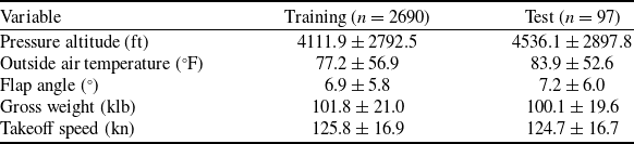
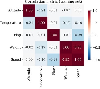
The data set used in this study was provided as two separate files. The first file contains the training data with 2,690 valid samples after the removal of one blank line, and the second file contains the test data with 97 samples. In contrast to the previous study [Reference Karaburun, Ark Hatipoglu and Konar26], in which the data set was split as 70% training and 30% test by random sampling, two separate files were used in this study. None of the 97 samples in the test file appears in the training file, and, therefore, the test evaluation is performed on completely unseen data. This is an important difference from the previous study and provides a more difficult generalisation evaluation. The descriptive statistics of the training and test subsets are presented in Table 1, and the correlation matrix of the input features and the takeoff speed on the training set is presented in Fig. 2.

Table 1.

The descriptive statistics of the training and test subsets (mean $ \pm $ standard deviation)

Figure 2.

The Pearson correlation matrix of the four input features and the takeoff speed on the training set.

A pre-processing pipeline was then assembled to prepare the records for the deep learning models. The training records were first inspected for missing entries and out-of-range values, and the few problematic rows were corrected or discarded. To ensure that all predictors enter the loss function at a comparable magnitude, each input feature was rescaled to zero mean and unit variance using the StandardScaler transformer from the Scikit-Learn library. The same affine transformation was also applied to the regression target so that the optimiser would operate on a numerically well-conditioned loss surface; at inference time, the scaler was inverted before the error metrics in Kn were computed. To prevent information leakage from the test partition, the mean and variance used by the scaler were estimated exclusively from the training subset and the resulting parameters were then re-used to transform the test subset.

After the pre-processing step, the training file was further split as 85% training data and 15% validation data by a single random holdout with a fixed seed of 42. This validation partition was used by the early stopping callback with patience of 40 epochs and by the learning rate scheduler that halves the learning rate when the validation loss has not improved for 15 epochs (with a minimum learning rate of ${10^{ - 5}}$ ). The Adam optimiser with an initial learning rate of ${10^{ - 3}}$ , a batch size of 64 and a maximum of 400 epochs were used in the training of all four base models. The TensorFlow 2.17 library [Reference Abadi, Barham, Chen, Chen, Davis, Dean, Devin, Ghemawat, Irving and Isard40] and the Keras Tuner library [Reference O’Malley, Bursztein, Long, Chollet, Jin and Invernizzi38] were used for the implementation of the deep learning models and the hyperparameter optimisation step. The Scikit-Learn library [Reference Pedregosa, Varoquaux, Gramfort, Michel, Thirion, Grisel, Blondel, Prettenhofer, Weiss and Dubourg41] was used for the pre-processing and the metric computation steps. The global NumPy and TensorFlow seeds were both fixed at 42 so that the reported metrics can be reproduced from the released training scripts.

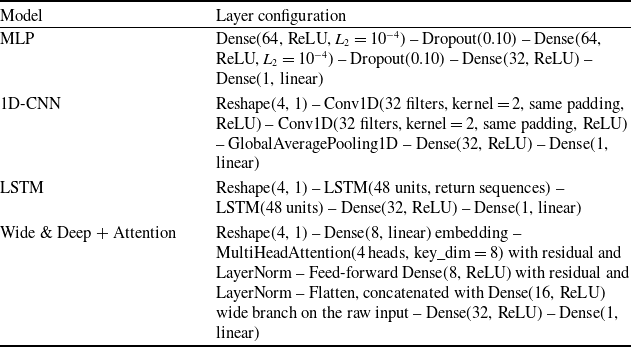
To make the four base architectures fully reproducible, the layer-by-layer configuration that was kept identical across all reported runs is presented in Table 2. The four predictors enter every model through the same standardised four-dimensional vector, and the three networks that operate on a sequence representation (1D-CNN, LSTM and the wide-and-deep network with self-attention) reshape this vector to a length-four signal with a single channel before the first internal layer.

Table 2.

Architectural configuration of the four base deep learning models used in this study

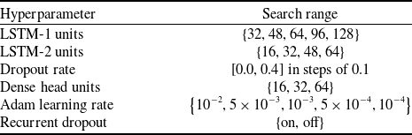
After the training of the four base models, the model with the smallest error value was selected for the hyperparameter optimisation step. The hyperparameters of the selected model and their search ranges are given in Table 3. Bayesian hyperparameter optimisation [Reference Shahriari, Swersky, Wang, Adams and de Freitas37] as implemented in the Keras Tuner library [Reference O’Malley, Bursztein, Long, Chollet, Jin and Invernizzi38] was applied to obtain the best hyperparameter combination. Each trial was trained on the 85% training partition with early stopping on the 15% validation partition. The validation MSE value was used as the objective of the Bayesian optimisation, and a total of 24 trials was used as the search budget. The hyperparameter combination with the smallest validation MSE was selected as the final tuned model, and the final model was re-trained with extended early stopping (patience of 60 epochs) before the evaluation on the test data.

Table 3.

The search ranges selected for the Bayesian hyperparameter optimisation of the LSTM model

4.0 Simulation results

The simulation outcomes obtained with the proposed deep learning pipeline are reported below in detail.

The experimental protocol was carried out exactly as described in Section 3. The Boeing 737-300 manual data [6] were taken as the working set, with pressure altitude, outside air temperature, gross weight and flap angle entering the model as predictors and takeoff speed acting as the regression target. Records were screened for missing entries and out-of-range values, each predictor was standardised through the Scikit-Learn StandardScaler transformer and the training corpus was further partitioned into 85% training and 15% validation subsets by random holdout with a fixed seed. The four candidate architectures – MLP, 1D-CNN, LSTM and the wide-and-deep network with multi-head self-attention – were then trained on the training partition under identical callbacks (early stopping and learning-rate reduction on plateau) and were finally evaluated on the held-out test file of 97 unseen samples.

Figure 3 shows the training and validation loss curves of the four base deep learning models during the training process. When Fig. 3 is examined, it is seen that the four models converge monotonically, and the validation loss curves follow the training loss curves. This indicates that the regularisation strategy applied during the training, which consists of dropout, ${L_2}$ weight decay and early stopping, was sufficient to prevent overlearning on the standardised four-feature input.

For takeoff speed prediction, the RMSE, MSE and MAE values of the simulation results obtained with the four base models on the test data are presented in Table 4. The trainable parameter count and the wall-clock training time of each model on a 3.10 GHz Intel Core i5-10500 CPU are also presented in Table 4.

Table 4.

The RMSE, MSE and MAE values of the four base deep learning models on the test data, with the trainable parameter count and the training time

Figure 3.

The training and validation loss curves of the four base deep learning models.

When Table 4 is examined, it is seen that the largest error metric value is obtained with the MLP model, while the smallest RMSE and MSE values are obtained with the LSTM model. The 1D-CNN model gave a slightly smaller MAE value than the LSTM model, but the RMSE values of the two models are very close and both are smaller than 0.8 kn. The wide-and-deep model with self-attention obtained an RMSE value between the MLP model and the 1D-CNN model. Considering the obtained results, the LSTM model gave the smallest RMSE and MSE values among the four base models and was selected for the hyperparameter optimisation step.

The comparison of the actual takeoff speed values and the predicted takeoff speed values for the four base models is presented in Figs 4 to 7, respectively, for the MLP, 1D-CNN, LSTM and wide-and-deep with self-attention models.

Figure 4.

Comparison of the actual takeoff speed values with the predicted takeoff speed values for the MLP base model.

Figure 5.

Comparison of the actual takeoff speed values with the predicted takeoff speed values for the 1D-CNN base model.

Figure 6.

Comparison of the actual takeoff speed values with the predicted takeoff speed values for the LSTM base model.

Figure 7.

Comparison of the actual takeoff speed values with the predicted takeoff speed values for the wide-and-deep model with self-attention.

When the figures comparing the actual takeoff speed values with the predicted takeoff speed values are examined, it is seen that the MLP model shows a discernible spread around the identity line, especially at the upper end of the speed range (above $\sim 140$ kn) where the test data samples lie far from the training grid. The 1D-CNN and the LSTM scatter plots are tightly aligned with the identity line. The wide-and-deep model with self-attention also follows the identity line but with a slightly higher dispersion compared to the 1D-CNN and the LSTM.

The residuals of the four base models versus the predicted takeoff speed values on the test data are presented in Fig. 8. When Fig. 8 is examined, it is seen that the majority of the residuals are concentrated within a $ \pm 1.5$ Kn band around zero, and there is no obvious sign of bias. A small number of larger residuals are observed at the high-temperature, high-weight corner of the operating envelope, which is consistent with the test data containing samples (for example, at $148{^ \circ }$ F and $155{^ \circ }$ F) that the models had to extrapolate to.

Table 5.

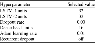
The best hyperparameter combination obtained with Bayesian optimisation of the LSTM model

Figure 8.

The residuals versus the predicted takeoff speed values for the four base deep learning models on the test data.

Figure 8. Long description

The image contains four scatter plots, each representing residuals versus predicted takeoff speed values for different deep learning models. Panel A: The scatter plot for the MLP model shows residuals on the vertical axis (in knots) and predicted takeoff speed on the horizontal axis (in knots). The data points are scattered around the zero residual line, indicating the model’s prediction errors. Panel B: The scatter plot for the CNN1D model also shows residuals on the vertical axis (in knots) and predicted takeoff speed on the horizontal axis (in knots). The data points are similarly scattered around the zero residual line. Panel C: The scatter plot for the LSTM model displays residuals on the vertical axis (in knots) and predicted takeoff speed on the horizontal axis (in knots). The data points are scattered around the zero residual line, showing the model’s prediction errors. Panel D: The scatter plot for the Attention model shows residuals on the vertical axis (in knots) and predicted takeoff speed on the horizontal axis (in knots). The data points are scattered around the zero residual line, indicating the model’s prediction errors.

After the comparison of the base models, the LSTM model was selected for hyperparameter optimisation to further improve the model performance. For this purpose, Bayesian hyperparameter optimisation as implemented in the Keras Tuner library was applied with the search ranges given in Table 3. A total of 24 trials with early stopping on the validation partition was used as the search budget. The best hyperparameter combination obtained as a result of the Bayesian optimisation is presented in Table 5.

Using the best hyperparameter combination, the LSTM model was re-trained with extended early stopping (patience of 60 epochs and a maximum of 600 epochs). The RMSE, MSE and MAE values of the tuned LSTM model and the base LSTM model on the test data are presented in Table 6.

Table 6.

The RMSE, MSE and MAE values of the LSTM model before and after Bayesian hyperparameter optimisation

When Table 6 is examined, it is seen that the Bayesian optimiser selected a more compact recurrent topology with LSTM-1/LSTM-2 widths of 32/32, a dense head of 16 units, no dropout, no recurrent dropout and an Adam learning rate of $0.01$ . The configuration delivered the smallest validation MSE among the 24 trials and was therefore retained as the tuned model. On the unseen test file, however, the tuned LSTM gave RMSE = 0.8164, MSE = 0.6665 and MAE = 0.4772 values, which are close to but slightly larger than the base LSTM values of RMSE = 0.7745, MSE = 0.5999 and MAE = 0.4527. The tuned model, therefore, did not transfer its validation improvement to the test set.

This validation-to-test gap is attributed to three concurrent factors. First, the 15% validation partition (around 404 records sampled from the training file) is drawn from the same distribution as the training records, whereas the 97-sample test file contains explicit extrapolation points at $148{^ \circ }$ F and $155{^ \circ }$ F that lie above the high-temperature tail of the training data. A configuration that minimises the in-distribution validation MSE is therefore not guaranteed to minimise the test MSE that includes the extrapolation samples. Second, the selected learning rate of $0.01$ is one order of magnitude larger than the base learning rate of ${10^{ - 3}}$ , and the absence of dropout makes the optimisation trajectory more sensitive to mini-batch noise. The combination of a smaller recurrent core, a higher learning rate and no regularisation can yield a validation-optimal weight configuration that sits in a sharper region of the loss surface, which transfers less reliably to the out-of-distribution test samples. Third, the search budget of 24 trials with a single execution per trial is modest by Bayesian optimisation standards, and a more robust protocol (for example, a $k$ -fold cross-validated objective or two-to-three executions per trial averaged over independent seeds) would harden the selected configuration against this source of variance. Considered together, the very close cluster of test RMSE values obtained by the 1D-CNN, the base LSTM and the tuned LSTM, all between 0.77 and 0.82 kn, indicates that the available four physical predictors place a practical lower bound on the achievable test error, and further architectural search alone is unlikely to push the test RMSE substantially below the base LSTM value reported here. A meaningful next improvement would require either richer input features (for example, runway slope or wind components from operational records) or a larger and more diverse test partition that better exercises the high-temperature, high-weight corner of the operating envelope.

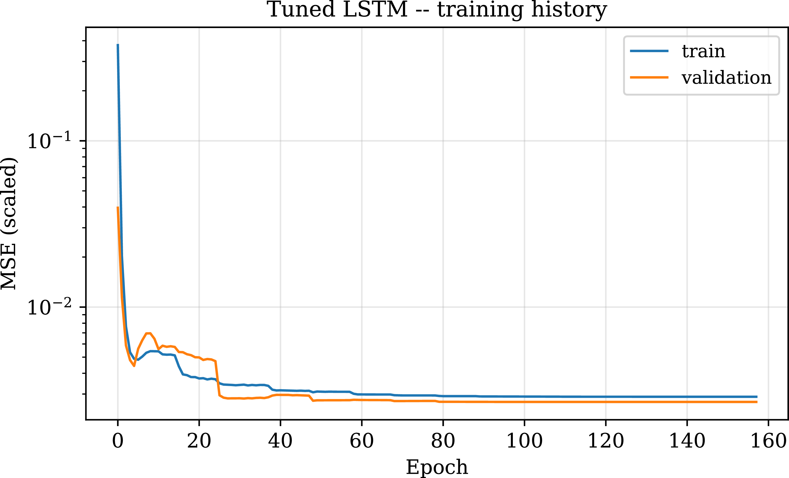
The comparison of the actual takeoff speed values with the predicted takeoff speed values of the tuned LSTM model is presented in Fig. 9, and the training and validation loss curves of the tuned LSTM model are presented in Fig. 10.

Figure 9.

Comparison of the actual takeoff speed values with the predicted takeoff speed values for the LSTM model after Bayesian hyperparameter optimisation.

Figure 10.

The training and validation loss curves of the tuned LSTM model.

When Fig. 9 is examined, it is seen that the tuned LSTM model shows satisfactory results on the test data. The predicted takeoff speed values are tightly aligned with the actual takeoff speed values along the identity line.

Beyond the aggregate error metrics, the generalisability of the proposed deep learning pipeline can be assessed along three complementary axes. The first is the alignment of the train and test distributions, which is summarised in Table 1. The mean values of the four predictors and of the takeoff-speed target on the 97-sample test file lie within roughly a quarter of one standard deviation of the corresponding training means, and the standard deviations themselves are comparable on the two partitions. This indicates that the test file exercises the central region of the same operating envelope on which the models were trained, and that the reported test errors are representative of normal operating conditions rather than of an artificially easy or an artificially hard subset. The second axis is the behaviour of the models on the explicit out-of-envelope samples that the test file does include, in particular the records at $148{^ \circ }$ F and $155{^ \circ }$ F that lie above the upper temperature tail observed during training. The residual plot in Fig. 8 shows that the larger absolute residuals concentrate at the high-speed, high-temperature corner of the operating envelope, while the majority of the predictions remain inside the $ \pm 1.5$ kn band. This is the expected fingerprint of a learned regressor that interpolates accurately inside the training support and degrades gracefully under mild extrapolation. The third axis is the structural protection against test leakage that was built into the pipeline. The training corpus was supplied as a separate file from the 97-sample test file, none of the test records appear in the training file, the standardisation statistics were estimated exclusively from the training subset and the early-stopping and learning-rate scheduling decisions were taken only on the 15% validation slice carved from the training file. The reported test metrics, therefore, reflect genuine generalisation to data that the models never observed during training or model selection.

These three observations support the use of the developed networks as a decision-support tool for the takeoff-speed prediction problem of the Boeing 737-300 within the operating envelope described in Section 3. The corresponding scope limitations should also be stated explicitly. The training corpus comes from the manufacturer’s chart-based operations manual [6] and therefore inherits the smoothness and the noise-free character of that source rather than the dispersion of actual flight measurements. The models were trained on a single airframe family and on four physical predictors, and their behaviour on a different aircraft or on operational QAR streams cannot be inferred from the present test errors. A direct transfer to flight-recorded data would require either a domain-adaptation step or a re-training pass on operational records.

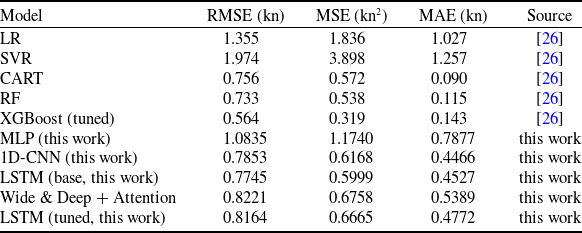
To evaluate the performance of the proposed deep learning models against the classical machine learning baselines, the comparison of the tuned LSTM model with the classical models reported in the previous study of Karaburun et al. [Reference Karaburun, Ark Hatipoglu and Konar26] is presented in Table 7. The classical model results were obtained on a 70/30 random in-sample split, while the deep learning model results were obtained on a separate test file in which all 97 samples are unseen during training. For this reason, the comparison should be read as indicative rather than as a strict, side-by-side benchmark.

Table 7.

The test error values of the proposed deep learning models in comparison with the classical machine learning baselines of Karaburun et al. [Reference Karaburun, Ark Hatipoglu and Konar26]

When Table 7 is examined, it is seen that the tuned LSTM model gave an RMSE value that is comparable to the best classical baseline model and significantly smaller than the LR and SVR baseline values. The deep learning models gave a higher MAE value but a more uniform residual distribution compared to the classical CART and RF models. The CART and RF models obtained an MAE value of around 0.1 kn on their in-sample test split, while the best deep learning models (1D-CNN, LSTM and the wide-and-deep model with self-attention) obtained an MAE value smaller than 0.55 kn on the test file in which all 97 samples are unseen during training. This is consistent with the general observation that gradient-boosted tree ensembles are particularly successful on low-dimensional tabular regression problems [Reference Karaburun, Ark Hatipoglu and Konar26], while deep learning models become competitive when the operating envelope must be extrapolated. As a result, the takeoff speed prediction problem with four input features lies in a regime where both families remain effective, and the selection between them can be made considering the deployment requirements. The LSTM model can be converted to TensorFlow Lite [Reference Abadi, Barham, Chen, Chen, Davis, Dean, Devin, Ghemawat, Irving and Isard40] for the edge inference, and the recurrent network can also absorb time-series telemetry data in future studies.