1. Introduction

Many ice-dammed lakes are known to drain in sudden subglacial floods, or jökulhlaups, on a quasi-regular basis. Such behaviour supports the concept that jökulhlaup systems are threshold-governed, that in these systems a flood initiates when the lake fills to a certain water depth (or pressure) which enables subglacial drainage to breach the ice dam. Because the flood durations are typically several days to several weeks, much shorter than the intervening periods when the lake refills, observed histories of lake level often show sawtooth cycles over the long term, with slow refilling punctuated by rapid drawdown in the floods (Fig. 1a). Understanding these cycles can help unravel the physical controls on flood timing and size, as well as other glacio-hydrologic effects of ice-dammed lakes. Here we build a theory for these cycles, using insights from nonlinear dynamical systems and a flood record from Merzbacher Lake, central Asia.

Fig. 1.

(a) Typical time series of the lake level in a jökulhlaup system. Each refilling stage may last months, years or decades, whereas flood events are abrupt (indicated by arrows). (b) Cartoon of a model lake showing our key mathematical symbols.

Previous studies have tackled diverse aspects of jökulhlaup physics, including flood thermomechanical evolution and the shape of flood discharge hydrographs (Reference NyeNye, 1976; Reference Spring and HutterSpring and Hutter, 1981; Reference ClarkeClarke, 1982, Reference Clarke2003; Reference NgNg, 1998), the dam-breach mechanism (Reference FowlerFowler, 1999), coupling of flood drainage with subglacial hydrology (Reference AndersonAnderson and others, 2003; Reference Flowers, Björnsson, Pálsson and ClarkeFlowers and others, 2004), sediment transport (Reference Fowler and NgFowler and Ng, 1996), and glacier flow (Reference Anderson, Walder, Anderson, Trabant and FountainAnderson and others, 2005; Reference Sugiyama, Bauder, Weiss and FunkSugiyama and others, 2007) and the elusive relationship between flood peak discharge and flood volume (Reference Clague and MathewsClague and Mathews, 1973; Reference Walder and CostaWalder and Costa, 1996; Reference Ng and BjörnssonNg and Björnsson, 2003; Reference Ng, Liu, Mavlyudov and WangNg and others, 2007). In contrast, the long-term rhythm of flood recurrence has received little attention, as only a handful of suitably complete records exist for study. Nonetheless, there are general expectations of how climate and glacier fluctuations might regulate the timing of jökulhlaups: a lake may outburst sooner if it receives meltwater faster under warm weather or if thinning of the ice dam lowers its flood-initiation threshold (e.g. Reference ThórarinssonThórarinsson, 1939). Consideration of the lake water balance, which underpins these ideas, forms the heart of our present analysis.

Figure 1b introduces our mathematical model. We envisage a marginal ice-dammed lake fed by a climate-dependent water supply (although the model can be easily adapted for subglacial lakes). If the lake has volume V and receives water at the rate Q _I, then its filling stage can be described by the equation

(1)

where t is time and h is the lake water depth. We assume that the ice dam prevents outflow from the lake while it refills, but when h reaches a critical threshold h _c (Fig. 1b) a flood initiates, draining the lake at once to a residual volume V ₀, i.e.

(2)

Our aim is to study the oscillatory cycles in this model, especially how their timing depends on Q _I and h _c, two factors which reflect environmental conditions.

The formulation in Equation (1) implies that one could forecast outburst timings by monitoring the lake depth h if the threshold h _c is known; h _c also represents an initial condition for simulating flood hydrographs and their peaks (Reference ClarkeClarke, 1982; Reference Ng and BjörnssonNg and Björnsson, 2003). At many lakes, however, the practical issue of predicting the next jökulhlaup is clouded by natural variations in h _c. It is often found that water depths at flood initiation differ from those needed to float the ice dam and that they vary markedly between floods. Uncertainty regarding how to prescribe the threshold also features in this study. The subglacial processes at flood initiation are notoriously difficult to observe, and insights on how to determine h _c remain few and indirect. Field monitoring by global positioning system has evidenced a strong mechanical coupling between ice dam and lake during flood initiation at Hidden Creek Lake, Alaska, USA (Reference Anderson, Walder, Anderson, Trabant and FountainAnderson and others, 2005; Reference WalderWalder and others, 2006), and Gornersee, Switzerland (Reference Sugiyama, Bauder, Weiss and FunkSugiyama and others, 2007). In terms of modelling, Reference FowlerFowler (1999) proposed a theory based on the Nye–Röthlisberger channel drainage equations to explain why the November 1996 Grímsvötn flood in Iceland began above flotation lake level.

In this paper, we use Equations (1) and (2) as a toy model to simulate multiple floods and explore their date sequences alongside the outburst record from Merzbacher Lake. Specifically we try to understand the structure of these sequences by disentangling the effects of meteorology (manifested in Q _I) and flood initiation (manifested in h _c), which are tunable inputs in the model. The simplifying assumption that h _c is constant is used in most of the early part of our investigations. Although the resulting model cannot seriously forecast the timing of individual floods, it reveals important principles behind their pattern. Our focus is theoretical, and we ask: What controls the temporal rhythm of flood cycles? What aspects of these cycles are predictable? Why might flood occurrence at a given lake cluster around a certain time of the year? Are there systematic differences that we can discern from the flood sequences of different lakes?

In sections 2 and 3 we introduce Merzbacher Lake and establish the climate forcing of our model. Section 4 performs key simulations and develops tools for analysing flood sequences, including an iterative map that links the dates of successive floods. At the end of that section, we relax the assumption of constant h _c and use the model to study the variable character of flood initiation at Merzbacher Lake. Conclusions follow in section 5.

2. Merzbacher Lake and its Jökulhlaups

Located in Kyrgyzstan, Merzbacher Lake is dammed marginally by the lowest 15 km of South Inylchek glacier, and lies at approximately 3250 m elevation at the lower end of the valley that harbours North Inylchek glacier (Fig. 2a). The lake contains about 0.2 km³ of water and is 80–100 m deep when full. Although we have no long-term record of the lake level, strandlines indicate that its earlier ‘highstands’ had been higher, consistent with the idea that the ice dam has thinned by tens of metres since the 19th century (Reference Glazyrin and PopovGlazyrin and Popov, 1999). A contour map of the lake bed has been made from stereophotogrammetry (Reference Kuzmichenok and DikikhKuzmichenok, 1984). Observations also suggest that the lake empties completely in each flood (V ₀ = 0) and that the ice-dam front position (hence lake geometry) has been stable (Reference MavlyudovMavlyudov, 1997). These properties, together with an exceptionally long jökulhlaup record, make the Merzbacher system a suitable case study. Since its discovery over a century ago (Reference MerzbacherMerzbacher, 1905), the lake has been visited by many expeditions and some of its floods have been reported in writing, mostly in Russian. A useful lead into this literature is provided by the papers of Reference Ayrapet’yants, Bakov, Shchukin and ZabirovAyrapet’yants and Bakov (1971), Reference MavlyudovMavlyudov (1997) and Reference Glazyrin and PopovGlazyrin and Popov (1999).

Fig. 2.

Location of Merzbacher Lake and its pattern of flood dates. (a) Map of central Tien Shan showing the lake (42°12′ N, 79°50′ E), North and South Inylchek glaciers, the Sary-Djaz river, Xiehela hydrological station, Tien Shan weather station, and approximate international borders. (b) Calendar dates of the floods plotted against the same dates represented on a continuous time axis. The best-fit straight line has a slope of −0.6 days a⁻¹. (c) Monthly flood-frequency histogram compiled from (b).

Merzbacher Lake has outburst almost every year since at least the 1950s (Reference LiuLiu, 1992; Reference Liu, Cheng and LiuLiu and others, 1998; Reference Shen, Wang, Shao, Mao and WangShen and others, 2007). Its floodwater follows the Sary-Djaz river across the Tien Shan and emerges in China near Aksu, a Silk Road oasis (Fig. 2a). This paper uses the data in Table 1, which lists the peak dates of 51 floods from 1956 to 2005 derived from the river-gauging records at Xiehela hydrological station near Aksu. Most of the peak dates have been identified from our collection of these records, which covers 90% of the years in the study period (we are missing 1956, 1957, 1973, 1974, 1975, 1994, winter of 1966, and summer of 1996). Other dates published by Reference LiuLiu (1992) and Reference Liu and FukushimaLiu and Fukushima (1999) cover the gaps in our collection and have been merged with our list. The list of dates in Table 1 is therefore as complete as possible to our knowledge. On the Xiehela discharge hydrographs, jökulhlaups are recognized by their shape (rapid rise, abrupt termination) or as major peaks unrelated to warm weather (thus we know that floods identified in May and June are not spring-melt events). As the discharge record has a sub-daily resolution, the peak dates are considered to be accurate to 1 day, but we acknowledge that several strongly diurnal parts of the record may contain floods that escaped identification. In section 3 we take care to neglect such periods from a calculation that relies on their absence.

Table 1.

Peak dates and estimated volumes of Merzbacher Lake jökulhlaups from 1956 to 2005 (our study period) derived from the river discharge record at Xiehela hydrological station, China. Volume errors are estimated from our hydrograph separation. Volumes in bold are used in the regression fit of Figure 3. As explained in section 2, other sources have provided peak dates that fill the gaps in our data collection: entry 40 comes from Reference Liu and FukushimaLiu and Fukushima (1999), and entries 1–3, 12 and 19–21 come from table 1 of Reference LiuLiu (1992) (which lists all pre-1989 dates). Symbols indicate consistency with dates reported elsewhere: ^* Reference KonovalovKonovalov (1990, table 1); ^† Reference MavlyudovMavlyudov (1997); ^‡ Reference LaiLai (1984, fig. 1)

Table 1 also gives the volume V _T of 19 floods estimated from each hydrograph’s area after its non-flood discharge component (‘base flow’) has been subtracted (see Reference Ng, Liu, Mavlyudov and WangNg and others, 2007, for details). We do not report the volume of the other floods, either because their large, diurnal base flow makes the estimation too uncertain, or because we do not have their hydrographic records (they fall inside the gaps mentioned above). Where a flood was witnessed in both Kyrgyzstan and China, the reported dates generally agree to ±1 day after allowing for time-zone difference, routing delay, and instances where reports documented different stages of the flood.

Figure 2b shows the complex timing of the floods. Their dates show large interannual variations and are not linked in any obvious way. On average they have occurred earlier in the calendar year by 30 days during the study period, although this trend is by no means statistically significant. Most years experienced a single flood; other years have either no flood (1960, 1962, 1977, 1979) or two floods (1956, 1963, 1966, 1978, 1980). A monthly flood-frequency histogram compiled from the dates is given in Figure 2c. It shows that most floods occurred in August and none from January to April, and there are minor peaks in May and December. We examine whether theory can predict flood sequences with similar characteristics to these.

3. Parameterization of the Lake Water Supply

Because weather and climate can strongly influence the lake water supply Q _I, we need a separate model to relate these forcings. Merzbacher Lake is fed primarily by snow- and ice melt from the two Inylchek glaciers, and much less by runoff from the basin sides and by rainfall. Additional input comes from the motion of South Inylchek glacier towards the lake, which, through calving at the ice dam, raises the lake level. Bearing in mind these contributions, we ignore rainfall here and assume an empirical model for Q _I (m³ d⁻¹) based on the temperature-index parameterization (e.g. Reference HockHock, 2003) and write

(3)

in which (x)₀₊ = max(x,0), T is the daily mean air temperature (°C), T ₀ is a temperature threshold for melting,k (m³ d⁻¹ °C⁻¹) measures the melt sensitivity to temperature, and a final term c represents the water-equivalent calving flux (assumed constant). Unlike sophisticated models, Equation (3) does not resolve ablation lowering, melt area and debris cover on melt surfaces separately. It also assumes that water is routed to the lake without delay.

We need plausible values of k, T ₀ and c. Although dedicated hydrometeorological measurements are lacking, it is possible to constrain these parameters with an argument of water balance that involves the lake’s long-term supply and the flood volumes in Table 1. In this method, we define a refilling interval as the period between the end of a flood and the end of the next flood, and we number this interval i if these floods are indexed i − 1 and i, respectively. We also denote the estimated volume of flood i by V _T,i. If each flood is assumed to end with an empty lake (as observations suggest), then flood i must evacuate all water supplied to the lake during the ith interval, denoted here by U_i , and we can equate V _T,i to U_i . The neglect from this balance of evaporative loss from the lake and precipitation on it (done also in Equation (1)) is justified for Merzbacher Lake. Now summation of Equation (3) over the interval gives

(4)

where p_i is the interval duration (days) and DD _i is the degree-day sum (days · °C)

(5)

Given p_i and DD _i data for a number of intervals, we can therefore treat U_i as a model of V _T,i and find k, T ₀ and c through multivariate regression (a non-linear problem due to the temperature cut-off). This method does not depend on the lake geometry or the flood-initiation threshold.

As inputs to the regression, 13 out of the 19 refilling intervals with V _T,i data (Table 1) are used because we believe each of them spans precisely two floods, with no extra floods draining the lake in between. The other refilling intervals are neglected either because they intersect with gaps in our Xiehela record or because they contain diurnal, high-discharge periods that may harbour unidentified floods (section 2). (Thus our determination of k, T ₀, c here should be conservative.) When compiling p_i data for Equation (4), we assume each peak date in Table 1 to be the last day of a flood and that a new refilling interval starts the next day. Potential errors in p_i should be <2 days. The compilation of DD _i in Equation (5) requires temperature data, and a possible source is the instrumental record (T _TS) at Tien Shan station about 120 km from the lake (Fig. 2a). However, since this record is often discontinuous before the 1970s, we use instead the surface temperature from the US National Centers for Environmental Prediction (NCEP)/US National Center for Atmospheric Research (NCAR) reanalysis, T _NCEP, which has daily coverage from 1948 to the present. The NCEP/NCAR reanalysis project uses data assimilation techniques that combine an atmospheric circulation model and many different sources of historical weather observations to estimate the past state of the atmosphere on a 2.5° × 2.5° latitude–longitude grid (Reference KalnayKalnay and others, 1996; Reference KistlerKistler and others, 2001). Here, T _NCEP is first interpolated to the position of Merzbacher Lake. Its variations should track temperature changes near the lake because the reanalysis and station records are strongly correlated where they overlap (T _NCEP = T _TS + 7.9; r ² = 0.90) and because T _TS reflects temperatures on South Inylchek glacier closely, although being offset from the latter by several °C (Reference Aizen, Aizen, Dozier, Melack, Sexton and NesterovAizen and others, 1997; Reference Aizen and AizenAizen and Aizen, 1998).

Rather than a single set of [k, T ₀, c] values, we use the regression method to find several parameter sets for driving the lake supply. This is not only because they enable useful comparisons, but because the general regression where k, T ₀ and c all need to be found is weakly determined; the high degree of freedom results in a good fit over wide parameter ranges. In order to overcome this problem, we use the regression together with independent observations of the ice flux c to design three parameter sets to cover a range of calving scenarios that bracket the real situation.

Table 2 lists our three parameter sets. From field measurements on South Inylchek glacier, Reference MavlyudovMavlyudov (1997) and Reference Mayer, Lambrecht, Hagg, Helm and ScharrerMayer and others (2008) estimated c at 0.014 and 0.012 km³ a⁻¹, respectively. Our first parameter set is just the result of the general regression (which ignores these estimates) and represents what we call a ‘high-flux’ case because its c value (0.045 km³ a⁻¹) is several times these estimates. The second parameter set uses the field estimates and is found from the regression with c fixed at 0.012 km³ a⁻¹. This yields the other two parameters

(6)

Table 2.

Parameters of Equation (3), corresponding to three different models of water supply to Merzbacher Lake and found by multivariate regression based on Equations (4) and (5)

and Figure 3 shows the match between V _T,i and U_i predictedby the corresponding lake water-supply model. We call this the ‘typical’ model, as it is most tightly constrained by available observations. A third parameter set, the ‘zero-flux’ case, is also derived from the regression, but with c = 0. The ‘typical’ scenario thus lies between the end-member cases. High r ² values in all three cases show that the temperature-index approach offers a valid description of melt generation, a finding supported by recent ablation measurements on the glacier (Reference Hagg, Mayer, Lambrecht and HelmHagg and others, 2008). Finally, we note that Reference Mayer, Lambrecht, Hagg, Helm and ScharrerMayer and others (2008) discerned seasonal variations in the flow of South Inylchek glacier, which may suggest a time-dependent model for c in future work. Such extension is ignored for now, however, since it would introduce parameters that are even harder for us to constrain.

Fig. 3.

Comparison of the observed flood volume V _T,i against the lake water supply volume U_i predicted by Equations (4) and (5) for 13 refilling intervals. Parameters used in the equations are those listed for the ‘typical’ calving scenario in Table 2.

4. Analysis of Flood Sequences

We proceed to study the temporal dynamics of the Merzbacher Lake system by simulating its filling history and comparing the simulated and observed flood sequences. Our complete model is now

(7a)

(7b)

where we calculate the lake water supply by using the sub-model

(8)

and Table 2 lists the [k, T ₀, c] values for three calving scenarios. Model inputs include the NCEP/NCAR temperature time series T _NCEP(t) and the lake geometry function h(V) compiled from Reference Kuzmichenok and DikikhKuzmichenok’s (1984) map. In our simulations, Equation (7a) is integrated on a daily time-step, with V being the lake volume at the start of each day; after daily filling, the depth h is updated with the new volume by looking up h(V), and we register a jökulhlaup whenever h≥h _c. This model envisages each flood to occur instantly with a volume V _c corresponding to the threshold water depth. The dates of simulated floods can be picked out from the solution V(t) or h(t).

Although Equation (7) looks simple, complex flood sequences can result from the interplay of water supply and the threshold, and it is useful to anticipate the key interactions. If both Q _I and h _c were constant, then the lake would, while filling, rise more slowly as it expands in area, but flood cycles would be periodic. Furthermore, unless the period is an integer multiple of a year, successive floods will land on different calendar dates. This solution may resemble the behaviour of subglacial lakes receiving steady basal melt (e.g. Grímsvötn at times with no volcanic eruptions) but is unrealistic for most marginal lakes, where Q _I varies with an annual temperature cycle. In fact, since marginal lakes may reach their threshold in different seasons, their filling cycles can fall out of step with temperature and become irregular. These cycles will be more complicated for lakes exhibiting h _c variations.

In this picture, annual cycles in Q _I pace the system asynchronously, and fast fluctuations of Q _I and h _c enrich the outcome. When trying to decipher flood date sequences, it therefore makes sense to assume a constant initiation threshold first, as done in sections 4.1–4.3. We remove this assumption later in section 4.4.

4.1. Model runs with a fixed threshold (h _c = constant)

Simulated time series

We have solved the model for each calving scenario, starting with the lake empty on 3 July 1956 (the day after flood 1 in Table 1) and ending in 2005. Lowering the threshold hastens flood return and raises the number of simulated floods, so we tuned h _c to obtain 51 floods as recorded, with the last flood matching its known date as closely as possible. The required h _c values are 88.2 m, 87.8 m and 87.7 m in the high-flux, typical and zero-flux scenarios respectively. The three corresponding solutions differ in detail, but share features exemplified by the typical model run which is illustrated in Figure 4.

Fig. 4.

Our ‘typical’ model simulation, based on a constant flood-initiation threshold h _c = 87.8 m and parameters listed for the typical scenario in Table 2. (a) The lake depth history h(t). This model run produced no flood in 1971 and 1989, and two flood events in 1958, 1968 and 2000. (b, d) Enlarged portions of (a) for two periods around 1971 (b) and 2000 (d). (c, e) Corresponding time series of temperature forcing T _NCEP and of the lake water-supply rate Q _I.

The lake depth history h(t) of this run (Fig. 4a) shows irregular sawtooth cycles, and Figure 4b–e zoom in to show how h(t) responds to temperature and water-supply forcing during two periods. (V(t) has a similar shape to h(t) and is omitted.) We see that temperature drives an annual meltwater cycle that peaks in the summer, when the fastest rise rate of the lake is of the order of 1 m d⁻¹, consistent with field observations (e.g. Reference MavlyudovMavlyudov, 1997). In contrast, cold weather (T _NCEP < T ₀) prevents melt generation during winter, when the lake gets stuck in a narrow range of depths (slow filling continues if c> 0). These winter stases as well as the jökulhlaups interrupt the filling cycles. And while the simulation is sensitive to the precise timing of these events and to weather fluctuations, it demonstrates a memory effect in the sense that one flood date influences the next. Winter stases are not apparent at subglacial lakes like Grímsvötn (Reference Guðmundsson, Björnsson and PálssonGuðmundsson and others, 1995, fig. 5) but probably occur at most marginal lakes.

Fig. 5.

(a) The pattern of flood dates simulated by our typical model. Recorded flood dates are included for comparison. (b–d) Monthly frequency histograms of the flood dates produced by the typical (b), high-flux (c) and zero-flux (d) model runs (coloured grey). Thick line in all three panels shows the recorded histogram. Wiggly curve in (b) shows the multi-year mean of the lake supply rate Q _I discussed in section 4.3.

The typical run also yields several no-flood years and dual-flood years, as seen at Merzbacher Lake. These anomalies may be viewed as missing beats and double beats respectively, because our tuning fits 51 floods into 50 years, implying a mean system period of close to 1 year. Figure 4b and c show that 1971 escapes a flood because the last flood comes late in 1970 and the 1971 melt season is relatively cold. On the other hand, we see from Figure 4d and e that two floods are simulated for 2000, as the first of these comes early enough in that year for the lake to regain the threshold before summer melt ends. Otherwise, successive floods normally span two calendar years and a winter. These results show that despite its irregularity, the flood sequence has a basic beat that depends on the strength of annual melt cycles. We will see that a crucial parameter of the system is the ratio of each year’s water supply volume to the flood volume (V _c).

Flood dates and flood frequency histograms

Although our model captures some of the observed dynamics, the simulated flood dates in all three calving scenarios fail to match the recorded dates (e.g. Fig. 5a). Parameter tuning did not resolve this problem, but the model is still promising. Both the recorded dates and those produced by the typical model run have a day-of-year range between 100 and 360 (Fig. 5a). The frequency histogram of this run also fits the observed histogram remarkably well (Fig. 5b). In contrast, the other runs do not simulate histograms with a peak in August, nor do they prevent floods early in the year or enable late (December) floods (Fig. 5c and d). While the non-linearity caused by the threshold means that the histograms do not vary smoothly with the parameters k, T ₀ and c, this comparison establishes the ‘typical’ scenario as our best description of lake water supply.

Figure 5 shows that the simulated histograms widen as the calving flux c increases, and this offers additional insight into the seasonality of floods. If c ≡ 0, floods cannot initiate during winter in the model because then the lake level is fixed; but if c > 0, not only can the winter lake level rise to the threshold to cause an outburst, the likelihood of this also increases with c. The calved ice raises the lake level whether it melts or not, as long as it becomes afloat. Indeed, one could conjecture that this input is what enables some marginal lakes to outburst in deep winters when they receive no (liquid) water. We will revisit some of these ideas when developing our theory later.

4.2. Mapping flood-sequence dynamics

Our lake is supplied water more or less continuously but drains episodically. A close analogy in the non-linear systems literature is the ‘dripping tap’, where the tap head is the reservoir, and leakage generates a drop sequence, akin to our flood sequence. The drop sequence becomes chaotic at high supply rates (Reference ShawShaw, 1984; Reference Martien, Pope, Scott and ShawMartien and others, 1985), and models of such behaviour (e.g. Reference D’Innocenzo, Paladini and RennaD’Innocenzo and others, 2006) have considered the fluid mechanics of drop formation and detachment, analogous to flood initiation.

The key matter of interest here is not whether the flood cycles are fundamentally chaotic, as we know that a chaotic forcing (weather) already limits their predictability. Rather, because flood cycles unfold in time in a way dependent on memory, it may be profitable to study their pattern via dynamical maps that relate one cycle to the next, as done in non-linear analysis (e.g. Reference DrazinDrazin, 1992). Two kinds of map are explored here using the Merzbacher flood dates and the results of the last section.

Time-delay maps

Most dripping-tap studies assume a constant water supply, and the resulting lack of a unique time frame leads to drop intervals being considered. If the drop time sequence is t ₁, t ₂, t ₃, . . ., and so on, then we may define the (refilling) intervals as p_i = t_i − t_{i −1}, and plotting p_{i +1} versus p_i gives a time-delay map. This notation agrees with how we defined p_i in section 3.

Figure 6 shows the time-delay maps of the recorded flood dates (Fig. 6a) and of the results of our three previous model runs (Fig. 6b–d). Each data point on these plots relates two intervals. The central cluster of points in Figure 6a indicates a tendency for the Merzbacher floods to stabilize their return period near 1 year. The typical (Fig. 6b) and zero-flux runs (Fig. 6d) reproduce this well, but not every other aspect of the observed map. In Figure 6a, data above and below the cluster indicate transitions from a normal (nearly annual) interval to intervals longer and shorter than a year, whereas data left of it indicate transitions from short intervals back to normal intervals. Figure 6b and d mimic these excursions, supporting the idea that melt variation could trigger irregular beats in the system, but they also predict long-to-normal transitions that are not observed. Some excursions in Figure 6a are not modelled at all. These include data near its right diagonal (p_{i +1} + p_i ≈ 730), which record asymmetric interval pairs spanning 2 years, and a data point near its top right corner, which records two long intervals ‘back to back’.

Fig. 6.

(a) Time-delay map of the recorded flood dates in Table 1. (b–d) Time-delay maps of the flood dates produced by the typical (b), high-flux (c) and zero-flux (d) model runs (dots). Grey crosses show data from (a) for comparison.

Calendar-date maps

The fact that our lake supply exhibits annual cycles suggestsa different map of system dynamics based on the calendardates of the floods. If τ_i is the day of year (DY) of flood timing t_i , we can plot τ_{i +1} against τ_i to relate two successive floods, as done in Figure 7a–d. These calendar-date maps are directly relevant to flood prediction because they show how each flood date jumps to the next.

Fig. 7.

Calendar-date maps of (a) the recorded flood dates in Table 1 and (b–d) the flood dates produced by the typical (b), high-flux (c) and zero-flux (d) model runs. In all panels, each symbol plots the dates of two successive floods. Symbols outlined by a circle indicate that the floods fall in the same year; symbols outlined by a square indicate that they span three calendar years; unenclosed symbols (dots, crosses) show that they fall in consecutive years. In (a), letters E, M and L refer to early, mid- and late season respectively, and the key right of the plot shows major types of seasonal transitions between successive floods.

The calendar-date map of the Merzbacher floods is shaped like a cross (Fig. 7a). Its data may be projected onto one of the axes to form the frequency histogram of Figure 2c. If we label the floods in DY130–DY190 as early-season (E), those in DY190–DY290 as mid-season (M) and those in DY290– DY366 as late-season (L), then these categories encompass the histogram peaks in May, August and December respectively, and the cross shape of the data shows that early- and late-season floods do not follow each other or themselves. We can also distinguish the data points according to whether each pair of floods falls (1) in the same year, (2) in successive years, or (3) across three calendar years (with a floodless second year), and Figure 7a plots these branches with different symbols. Together these classifications allow us to identify five major transitions in the data: M → M (the cross centre), M → L, L → M, M → E, and E → M (the cross’s four limbs), as explained by the key on the right of Figure 7a.

Interestingly, the first three transitions enable cycling between mid- and late-season floods (M and L) in successive single-flood years, with M → M being the norm. But Merzbacher Lake, like a child playing hopscotch who trips over occasionally, sometimes escapes from this pattern via the last two transitions. Specifically, M → E yields an early-season flood after skipping a calendar year (a missing beat), whereas E → M recovers the normal pattern by precipitating a dual-flood year (a double beat). Such pairing of years occurred in 1962/63, 1977/78 and 1979/80. In Figure 7a, these instances involve data points in the cross’s lower limb (outlined by squares) and left-hand limb (outlined by circles). The two kinds of structures in the recorded flood sequence discussed here are intriguing and hard to discern from Figure 2b.

The simulated calendar-date maps (Fig. 7b–d) mimic the observed map with varying success. All three runs generate flood pairs in roughly the right areas, with branch 1 data in τ_{i +1} > τ_i , branch 2 data near τ_{i +1} ≈ τ _i and branch 3 data in τ_{i +1} < τ_i . The typical and zero-flux runs (Fig. 7b and d) are again better than the high-flux run at matching the observations, but some flood events which they predict for single-flood years come very early in the year. These runs also have trouble simulating late-season floods (and their transitions from/to mid-season floods), although the typical run manages to yield a couple of November and December outbursts. This comparison supports our conclusion that the model with ‘typical’ parameters qualitatively resembles the real system.

4.3. Theory of flood-sequence generation

Inspired that our toy model may bear clues to the structure of flood sequences, here we ask how its operation governs the dynamics on the calendar-date map. We advance a theory where time t (years) aligns with the calendar and the lake supply is annually periodic, i.e. Q _I(t) = Q _I(t + 1). (For Merzbacher Lake, one may construct such forcing from the long-term climatological mean of T _NCEP) Figure 8a shows a typical form of Q _I(t) for lakes in the Northern Hemisphere, with the melt peak in May–September. Integrating Q _I(t) with respect to time gives the cumulative lake supply volume

(9)

Fig. 8.

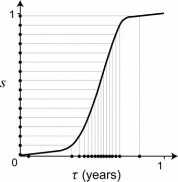
Basis of asynchronous pacing of floods in a model jökulhlaup system. (a) A periodic water supply rate Q _I(t). (b) The lake’s cumulative supply volume m as a function of time. For a constant flood volume V _c, flood events (shown as dots) are equally spaced in m but irregularly spaced in time, as indicated by the arrows on both plot axes. (c) The normalized function s(t) derived from a unit cell in (b).

whose graph consists of repeating wiggles that reflect water addition by each year’s melt cycle (Fig. 8b).

The cumulative volume m helps us understand how a flood sequence unfolds because each flood drains some of it. If the floods empty the lake completely and their initiation threshold is fixed, then their volume V _c would be constant, and the model predicts an outburst whenever the lake receives this volume. In Figure 8b we can think of the m axis as being partitioned equally by the floods (horizontal arrows) such that m_{i +1} = m_i + V _c, if we index the floods as before; the curve m(t) then converts this sequence into irregular timings on the t axis. These graphical relationships outline the basic mechanism behind asynchronous pacing of multiple floods.

To develop this theory, we need to track where flood events land on the curve m(t). Each flood’s position in a melt cycle may be described by how much water has been supplied to the lake that year, i.e. by how far up it lies on a wiggle. If we use m(t) in 0 ≤ t ≤ 1 to define the functional shape of each wiggle, μ(t) (dashed box, Fig. 8b), then the variable μ measures the volumetric progress of a melt cycle, and the annual total supply volume equals μ(1). Hence we may list the flood positions as the sequence μ ₁, μ _2, μ ₃,…. Below, we define the (normalized) variable s(t) = μ(t)/μ(1) (Fig. 8c) to form an alternative list s ₁, s ₂, s ₃, … where 0 ≤ s_i ≤ 1. On this list, each flood’s position is represented by the fraction of annual total water supply received by the lake by the time of the outburst.

The generation of multiple floods now works as follows. Since a constant flood volume V _c separates them on the m axis, we can deduce μ ₂ from μ _1, μ ₃ from μ ₂, and so on. Notably, μ_{i +1} is the residual of μ_i + V _c after multiples of the annual supply volume μ(1) have been subtracted; thus successive floods have different positions if V _c ≠ μ(1). Suppose V _c < μ(1), as in Figure 8b’s example. If flood i comes very early in a melt cycle, then the lake will refill before the end of the cycle to deliver flood i + 1 (which therefore falls in the same calendar year). If flood i comes late enough in the cycle, then flood i + 1 will arrive in the next melt cycle (next year) but earlier in the cycle. These relations between successive floods may be summarized

by writing

(10)

or, after normalization (dividing everything by μ(1)),

(11a)

(11b)

where we have introduced the flood recurrence parameter

(12)

ϕ represents the mean flood-return period of the system(years), and its reciprocal is the mean flood frequency (a⁻¹).

Given an initial value s ₁, Equation (11) can be iterated to form the sequence s ₁, s ₂, s ₃, … and we can plot s_{i +1} versus s_i to show this on what we call the generator map. Figure 9a gives an example of this map involving eight floods and seven flood pairs (numbered points). Its upper and lower branches (bold lines) are the loci of flood pairs spanning the same year and consecutive years, respectively, as defined by Equations (11a) and (11b). The iteration orbit can be traced with the help of the line s_{i +1} = s_i . Equations (10) and (11) are valid for ϕ ≤ 1, but we consider other cases below.

Fig. 9.

(a) The generator map when the recurrence parameter ϕ < 1.The variable s describes a flood’s position within an annual water-supply cycle, in terms of the fraction of the annual total supply volume which the lake has received when the flood occurs. Each point on the map (s_i , s_{i +1}) relates two successive floods in a sequence. The thick lines plot the branches of Equation (11), the dashed line is s_{i +1} = s_i , and arrowed trajectories show forward iteration of the map. (b, c) The function s(τ) from Figure 8c, positioned to transform s on both generator axes into calendar time τ. (d) The calendar-date map (τ_{i +1} versus τ_i ) resulting from the transformation. The axes are rotated from those in Figure 7. Points that plot the timing of flood pairs mirror the points in (a) and are numbered correspondingly. The curves are transformed versions of the branches in (a).

The conversion described earlier may now be used to turn s ₁, s ₂, s ₃, … into flood dates τ ₁, τ ₂, τ ₃, … via a variable change defined by the curve s(τ) in Figure 8c. (The requirement that s(τ) is monotonic to make this unique is satisfied by our ‘typical’ model for Merzbacher Lake because its non-zero calving flux ensures Q _I > 0.) Figure 9a–c show how the generator map can be transformed in this way to yield the calendar-date map (Fig. 9d). The iteration orbit on the latter map mirrors the generator orbit in Figure 9a but is governed by two curved branches (defined implicitly by Equation (11) and s(τ)). Figure 9 shows that while flood sequences may obey relatively simple generator dynamics, the non-linear form of s(τ) complicates their imprint in time. We consider the ramifications of this theory below.

Effect of ϕ on the generator sequence (s₁, s₂, s₃, …)

The recurrence parameter ϕ controls the properties of the generator map, and ϕ = 1 marks a key transition. If ϕ < 1, the lake needs only part of the annual supply volume to outburst, so multi-flood years (but no zero-flood years) may arise in the flood sequence, and the upper branch in Figure 9a reflects this possibility. If ϕ > 1, refilling to the threshold requires more than 1 year’s supply, so the sequence will consist of zero- and single-flood years only. Repeating our derivation in this case yields the generator equations

(13)

where and is the highest integer below ϕ. (This result is a generalization valid for all positive ϕ and includes Equation (11).) Figure 10 shows the corresponding generator map and calendar-date map, where the upper and lower branches advance time by and calendar years, respectively.

Fig. 10.

(a) The generator map when ϕ > 1 and (b) the corresponding calendar-date map. As in Figure 9, numbered points in both panels relate paired events of a sample flood sequence. In (a), thick lines plot the branches of Equation (13) and ϕ ^* is the decimal part of ϕ (that is, if is the highest integer below ϕ).

Mathematically, the sequence s ₁, s ₂, s ₃, … is just the decimal part of the numbers s ₁, s ₁ + ϕ, s ₁ + 2ϕ, …. This realization implies that the generator map will not be chaotic if ϕ is constant, and that s_i in long flood sequences will be uniformly distributed (between 0 and 1) if ϕ is irrational, but periodic if ϕ is rational. We expect variations of ϕ in real systems to rule out the latter behaviour.

Seasonality of flood events

Consider next the flood timings. Intuitively, outbursts are more likely to occur when high supply rates fill the lake quickly. Seasonal variations in Q _I should therefore cause an uneven spread of flood dates in the year and control their frequency histogram in a predictable way. We can quantify this idea using the framework in Figures 9 and 10.

The S shape of s(τ) is due to intense meltwater supply during summer and low supply during winter (Fig. 8c). Because the slope ds/dτ is large near τ ≈ 0.5, most (s_i , s_{i +1}) pairs on the generator map are transformed as date-pairs near the centre of the calendar-date map, where the two branches bend sharply (Figs 9 and 10). Flood dates will therefore focus in the summer if the sequence s_i is uniformly distributed. A cartoon of this effect (Fig. 11) allows us to deduce that the probability density function P(s) ≡ 1 leads to

(14)

Fig. 11.

Focusing effect of the transformations in Figures 9 and 10.Due to the curve shape of s(τ), a uniformly distributed set of s valuesturn into τ values that densely populate the summer part of the year.

which means that the flood frequency histogram will resemble the supply function Q _I(τ) and peak when it is highest. This result is exact if the generator sequence is uniformly distributed and infinitely long.

To test it for Merzbacher Lake, we took the T _NCEP(t) time series of each year in our study period and averaged them to find a mean annual temperature cycle. We then used this cycle as input in Equation (3) (with typical parameters) to estimate the long-term mean of Q _I(τ), and overlay this annual supply distribution in Figure 5b (shown by the wiggly curve). The shape of Q _I(τ) approximates both the recorded and modelled histograms, with the latter correspondence being closer probably because our ‘typical’ model used a constant outburst threshold. These agreements are impressive, as the histograms in this comparison are not ideal: they log relatively few samples (51 floods) and carry variations in ϕ (see next) not accounted by Equation (14).

Equation (14) also explains an effect of the calving flux c that we saw in the simulations of section 4.1. If c is much smaller than the summer melt peak, the probability of winter floods P(τ ≈ 0, or 1) is so low that they may not occur in a short flood sequence, and the likely result is a narrow histogram. If c is large, Q _I will have negligible seasonal variations, and Equation (14) predicts a flat (and wide) histogram.

Natural variability

How do climatic and glaciological factors influence flood temporal dynamics in this theory? In real systems, weather fluctuations alter Q _I(t) from year to year, and this ‘blurs’ the flood dates on the calendar-date map via the s–t transformation (e.g. in Fig. 9b and c). However, natural changes in the recurrence parameter ϕ may also affect the outcome directly by shifting the branches of the generator map (in Figs 9a and 10a).

Equation (12) identifies numerous potential factors behind ϕ. In its denominator, the annual water supply μ(1) depends on weather through the year (meteorological temperature) and the calving flux (influenced by glacier motion); in its numerator, the flood volume V _c depends on the outburst threshold and the lake geometry, both of which may vary with the ice-dam position. Hence, changes in ϕ may have diverse origins. In a hypothetical example, prolonged climatic warming may cause a given lake to receive more water (via enhanced melt generation) and lower its outburst threshold (via glacier thinning) each year. In this case, ϕ decreases, the mean flood frequency rises over time, and the generator branches (in Figs 9a and 10a) move towards the lower right as the flood sequence plays out on the map, raising the proportion of years with a high number of floods. The branches of the calendar-date map (e.g. Figs 9d and 10b) will shift accordingly, but in a way dependent on changes in s(τ) as well as in ϕ.

It is difficult to determine precisely how ϕ varied at Merzbacher Lake by such breakdown because we have reliable V _c data for only 19 floods, but we think the theory explains the broad structure of the observed calendar-date map (Fig. 7a). For the floods in our study period, an estimate of the mean flood volume is V _c = 1.6 × 10⁸ m³, if we assume the known lake geometry and the threshold h _c = 87.8 m inferred from the ‘typical’ simulation of section 4.1. Moreover, integration of the average supply function Q _I(τ) (see Fig. 5b and Equation (14)) gives μ(1) = 1.55 × 10⁸ m³. The mean recurrence parameter of Merzbacher Lake is therefore ϕ = V _c/μ(1) ≈ 1.0. Although this estimate contains errors, it is close enough to unity for us to expect natural variations to have flipped the system between ϕ < 1 and ϕ > 1, so that its calendar-date map becomes an amalgamation of Figures 9d and 10b. When ϕ < 1, the branches of Figure 9d show that flood pairs fall in either the same year or consecutive years; when ϕ > 1 (but <2), the branches of Figure 10b show that flood pairs either fall in consecutive years or span an additional year. This combination explains why the observed map (Fig. 7a) records data on all three branches (flood pairs falling in the same year, in successive years, and across three calendar years), with the second of these sandwiched between the other two.

Irregularity of jökulhlaup sequences

The considerations of the previous subsection prompt us to ask how the recurrence parameter ϕ governs the irregular rhythm of (long) flood sequences, in terms of their proportion of years that experience no flood, one flood, two floods and so on.

Although this problem could be studied on the generator map, a more direct method is to examine the ways whereby flood events fit into a (volumetric) melt cycle. Assume first that ϕ does not vary with time. We recognize three possibilities as the mean flood frequency n = 1/ϕ takes different values in a system. If n is an integer, then exactly n floods will occur at the same positions in every melt cycle and every year. If n < 1 (because ϕ > 1), then some cycles will be flood-free, while all remaining cycles will receive one flood. In this case, a period of N years (where N is large) yields N/ϕ floods, so the number of zero-flood years is N − N/ϕ, and the proportions f of zero-flood years and single-flood years are

(15)

where subscripts 0 and 1 indicate the year type. A third possibility is that n is a non-integer greater than 1. In this case, if denotes the largest integer below n, then one can show graphically that each melt cycle contains either or floods (Fig. 12). Further, if all flood positions s are equally probable, then the misfit between the cycle and flood volumes can be used to deduce that the ratio of -flood years to -flood years is (see Fig. 12). The proportions of these year types are thus given by

(16)

Fig. 12.

Positioning of multiple floods in a volumetric melt cycle (0 < s ≤ 1) when the recurrence parameter ϕ of the system is constant. Each dot represents a flood. (left) Reference sequence and our parameter definitions. If 1/ϕ is non-integer and is the highest integer below 1/ϕ, then a maximum of n complete refilling intervals fit into the melt cycle. Two year types are hence possible: (a) a year containing floods, caused by a slight left shift of the reference sequence, and (b) a year containing floods, caused by a slight right shift of the reference sequence.

This result is in fact applicable for all values of ϕ (> 0)because it reduces to Equation (15) when ϕ> 1 .

Figure 13 shows the proportions of different year types found from numerical simulations that used Equation (13) to generate long flood sequences. The simulated boundaries agree with the analytical result in Equation (16). These findings establish that when ϕ is constant, the flood sequence consists of no more than two year types, and the year types are characterized by the integer values closest to 1/ϕ.

Fig. 13.

Proportion of different year types in a long flood sequence, plotted against the recurrence parameter ϕ. Bars above the plot indicate the estimated ranges of variation of ϕ for Merzbacher Lake, Gornersee and Grímsvötn.

For a real system that exhibits variations in ϕ, Figure 13 still offers a useful classification of the flood sequence. For example, three year types (zero-, single- and dual-flood years) occur in the Merzbacher flood record, and their frequency ratio 0.08 : 0.82 : 0.1 may be used to infer the range of variation of ϕ about its mean (1.0): we can use the domains of Figure 13 with the knowledge that as much as 8% of the years had no floods and as much as 10% had two floods to define the lower and upper ends of this range (see the bar above the plot). Figure 13 also shows the estimated range of ϕ for two other lakes: Gornersee (which is ice-marginal) and Grímsvötn (which is subglacial). The Gornersee record from 1951 to 2005 shows 6 zero-flood years and 49 single-flood years (Reference Huss, Bauder, Werder, Funk and HockHuss and others, 2007), so f ₀ = 0.11, f ₁ = 0.89, and ϕ = 1.12; because dual-flood years are absent, we infer that ϕ did not fall below 1 and its variation was limited. The Grímsvötn record is more complex. Its flood return period was 5–7 years from the 1940s up until the November 1996 jökulhlaup, but decreased to about 1 year after that extraordinary flood (Reference BjörnssonBjörnsson, 1988, Reference Björnsson2002). While this change in behaviour has been associated with a sudden switch in the lake’s external controls (lowering of its flood-initiation threshold by tens of metres and increased geothermal activity) such that pre-1996 Grímsvötn and post-1996 Grímsvötn could be regarded as two different lakes, the considerable range of ϕ (≈ 1–7) and the resulting year types in this system are still useful indicators of its variability.

4.4. Modelling with a variable flood-initiation threshold

Despite the preceding theoretical insights, model Equation (7) cannot be used to reproduce or forecast flood dates accurately unless we supplement it with a model of flood initiation where h _c varies realistically. Our knowledge of the required physics is too limited to build such a model, but we can combine the data and model of this paper to study the behaviour of Merzbacher Lake’s threshold empirically.

We do this by first reconstructing the lake depth history h(t) for each refilling interval, the beginning and end of which are given by successive flood dates (Table 1). The toy model is solved in a different way from before. For each pair of successive floods we integrate Equation (7a) forward, starting with an empty lake 1 day after the first flood date and ending on the second flood date. The outburst condition in Equation (7b) is ignored to allow uninterrupted filling in each interval. The lake supply is still calculated from Equation (8) with T _NCEP data as input, and we adopt ‘typical’ [k, T ₀, c] values only. Figure 14 shows the simulated depth history when the results from different intervals are pieced together. As far as we know, it is the first such reconstruction for Merzbacher Lake. The peaks of h(t), which provide estimates of the initiation thresholds of the floods, fluctuate in the range 60–120 m.

Fig. 14.

The depth history of Merzbacher Lake reconstructed for our study period using the method described in section 4.4.

Do these variations depend on factors linked to the glacier and the lake? Here we explore this question by supposing a linear model for the threshold

(17)

where h _c0, β ₁ and β ₂ are constants. This model relates possible dependences of h _c on time t (referenced to the beginning of 1956) and on the lake-level rise rate dh/dt that could be speculated from two arguments. First, jökulhlaups have been thought to initiate by flotation when the lake depth reaches approximately 90% of the ice-dam thickness (see discussion by Reference NyeNye, 1976). Although this theory does not always accord with observations, the dam thickness may set the typical scale of h _c on which threshold variations are superimposed, so that long-term thinning of South Inylchek glacier (Reference Glazyrin and PopovGlazyrin and Popov, 1999) induces a falling trend in h _c (and then β ₁ > 0 in Equation (17)). The second argument concerns the role of the water depth h and the associated pressure in the sub-dam drainage during flood initiation. Since the threshold h _c defines the value of h at flood initiation, it cannot be a function of h itself but may depend on dh/dt if the drainage involves rate-dependent processes; h _c then varies as the lake fills. Such a dynamic threshold features in the flood-initiation mechanism of Reference FowlerFowler (1999), who envisages a mobile hydraulic divide under the dam as the ‘seal’. In his theory, the faster the lake level rises, the higher is the lake level when the divide finally reaches the lake to trigger a flood, and this explains the high initiation level of the 1996 Grímsvötn flood. Such behaviour would be mimicked by Equation (17) if β ₂<0.

To test Equation (17), we look for correlations that support the dependences suggested above, among data of h _c, t and dh/dt extracted from the peaks in Figure 14. Initiation of the Merzbacher floods preceded their recorded peak dates, as they have durations ranging from 4 to 18 days (Reference LiuLiu, 1992). Each reconstructed peak of h(t) in Figure 14 thus accounts for water supplied to the lake during the flood, and overestimates the actual lake ‘highstand’ that one would see at flood initiation. To correct for this approximately, here we extract h _c and t on the seventh day before each peak and relabel h _c as an ‘estimated threshold’, h _ce. (The 7 day offset is based on the mean length of the floods’ rising phase estimated from their hydrographs.) We also calculate dh/dt from the average slope of h(t) over a 5 day period ending on the same day, in order to make our results less sensitive to sudden (especially daily) fluctuations in the rise rate. The averaging period has been chosen to be longer than 1 day but not much longer than the flood duration, since the latter indicates a plausible timescale of coupling of the lake with sub-dam drainage.

Figure 15 shows the extracted data by plotting h _ce against t and dh/dt separately. The threshold has no significant time trend but seems to decrease with the lake-level rise rate, and this relation improves if we omit an outlier point. Proper fitting of Equation (17) to the data by multivariate regression confirms these observations and yields h _c0 = 97 m, β ₁ = −0.07 m a⁻¹ and β ₂ = 46 days (with r ² = 0.28) if all data are used, and h _c0 = 102 m, β ₁ = −0.03 m a⁻¹ and β ₂ = 58 days (with r ² = 0.46) if we omit the outlier. The last result hints at the description

(18)

where the threshold drops by several metres for each 0.1 m d⁻¹ increment in the rise rate. Interestingly, while the correlation supporting β ₂ > 0 is not strong, our data show no signs of the (opposite) behaviour predicted by Reference FowlerFowler’s (1999) theory (β ₂ < 0). This conclusion is unchanged when our choices of averaging period and offset are varied within reasonable bounds. We cannot address at this stage whether a given lake threshold ought to stiffen (β ₂ < 0) or weaken (β ₂ > 0) and indeed whether both types of behaviour could arise in different systems. But this analysis motivates the search for similar descriptions for the threshold of other lakes, as they may reveal patterns that shed light on the elusive mechanism of flood initiation.

Fig. 15.

Search for factors behind the estimated initiation threshold (h _ce) of 50 Merzbacher floods. (a) h _ce against the time of flood initiation. The best-fit regression line ignores dependence on dh/dt. (b) h _ce against the rate of lake-level rise dh/dt just before flood initiation, showing a systematic lowering trend. Solid line shows the best-fit regression of all data points; dashed line shows the regression with the outlier neglected. Both regressions ignore time dependence.

5. Conclusions

We have put forward a framework for studying the timing sequence of multiple subglacial floods, with an emphasis on floods from marginal ice-dammed lakes. Recorded flood dates from Merzbacher Lake are used as test data, and we found that a simple model of lake filling and drainage that assumes an outburst threshold (h _c) in the lake depth could capture some of the observed dynamics (sections 4.1 and 4.2). Theoretical analysis of this low-order model then exposed the clockwork nature of jökulhlaup systems (section 4.3). A key reason for an erratic sequence of flood dates is that refilling of the lake falls out of step with its annual cycles of water supply. The timing relationship of successive floods may be followed on non-linear maps (Figs 9 and 10), and these maps show that the flood-sequence structure depends critically on a dimensionless parameter ϕ ( = flood volume ÷ the lake’s annual supply volume). The same theory clarifies how environmental factors influence the irregular rhythm of such a sequence and explains how seasonal variation in the lake water supply controls the flood-frequency distribution on the calendar.

Section 4.4 presented a reconstruction of the filling history of Merzbacher Lake and used it to derive an empirical recipe for its variable threshold. This led to tentative evidence that flood initiation may be easier at Merzbacher Lake when it fills quickly, as summarized by Equation (18). Such a dynamic recipe might enable useful operational forecasts of the flood timings; notably, one could integrate it with our toy model, for example,

(19)

(20)

where

(21)

to see if the resulting model can successfully simulate the observed flood-date sequence. These ideas will be taken up elsewhere. Meanwhile, we have demonstrated that besides observing and modelling what goes on under the ice dam, one could probe the secrets of flood initiation by studying the timing pattern of floods: a macroscopic approach.

We have conceptualized jökulhlaup lakes as oscillatory systems and used the tools of non-linear dynamics to unravel their physics. Future work could explore several things in this context. First, our ‘generator map’ theory in section 4.3 may be extended to explain the higher-order dynamics that a changing flood-initiation threshold injects into the model; removing the assumption that the lake empties completely in each flood adds another level of complexity. This problem finds an analogy in the dripping tap (section 4.2), where the precise detachment process of a drop affects the timing and size of the next drop. A related challenge is to link any systematic behaviour shown by the threshold with the microphysics of flood initiation. Finally, there is the exciting possibility of repeating the analysis in this paper for other lakes and comparing their outburst sequences. The discovery of common clockwork behind them is in its infancy, but an understanding is emerging.