


Introduction
Revenue programs in the commodity and crop insurance titles of the farm bill are arguably the most popular subsidized risk management tools available. The 2014 farm bill and the succeeding 2018 farm bill offer Agriculture Risk Coverage at the county level (ARC-CO) under the commodity title (Title I), while Revenue Protection (RP) crop insurance under the crop insurance title (Title XI) has been offered, in one form or another, since 1996 (Dismukes and Coble, Reference Dismukes and Coble2007). Roughly 92% of corn and 96% of soybean base acres were enrolled in ARC-CO (USDA-FSA, 2018), while 91% of corn and soybeans acres enrolled in traditional crop insurance programs (i.e., YP, RP, RP-HPE) were enrolled in Revenue Protection crop insurance (USDA-RMA, 2018).
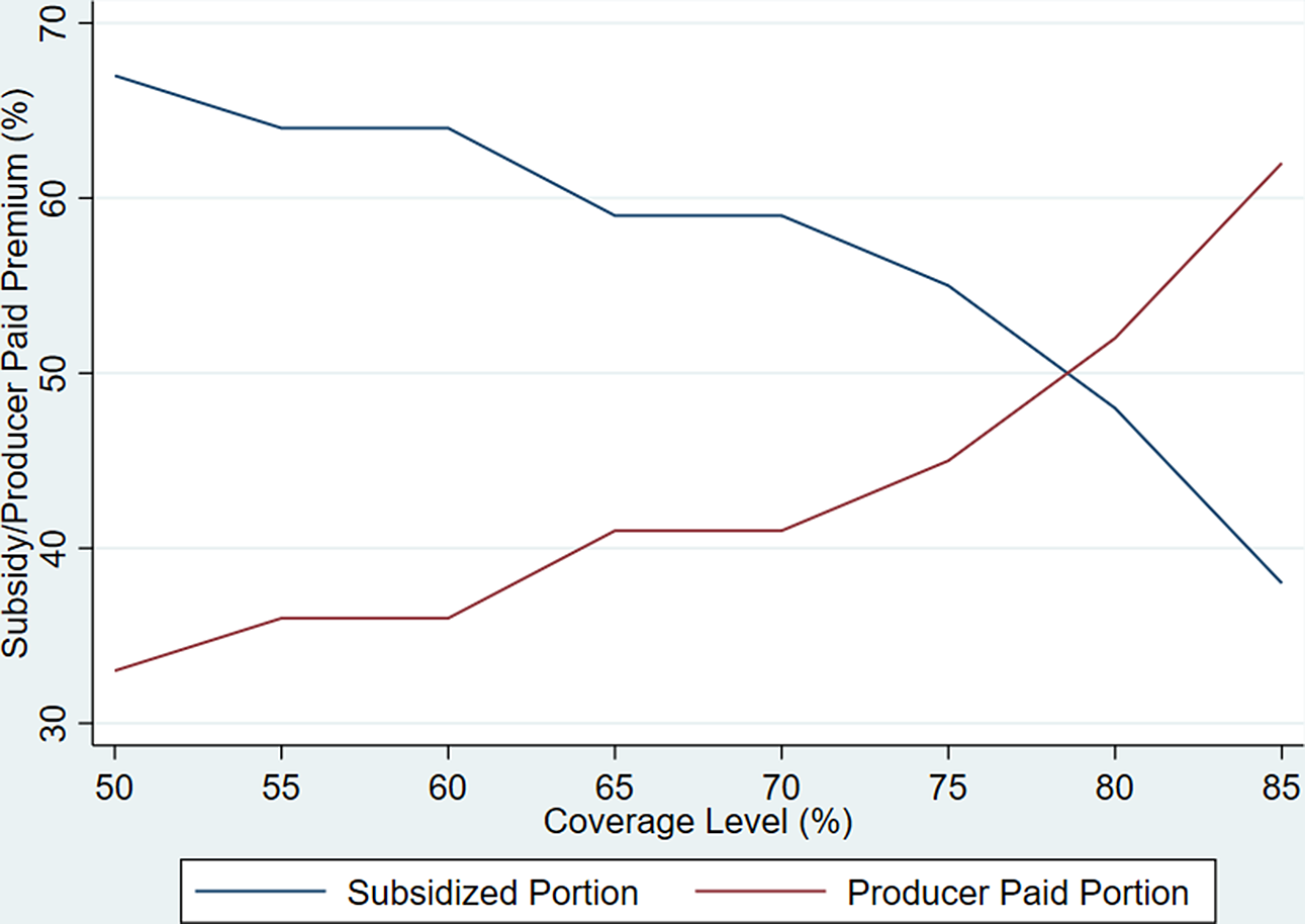
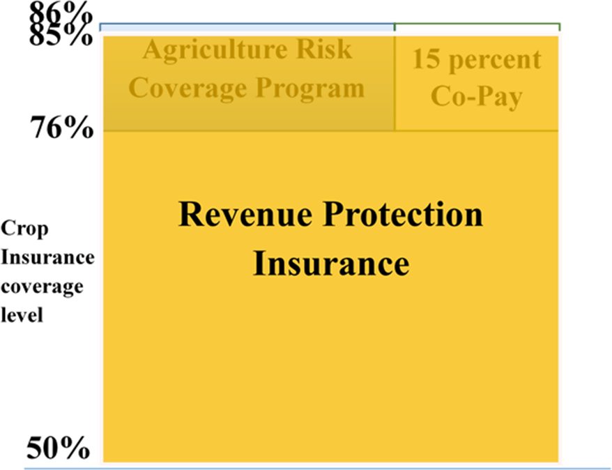
ARC-CO,Footnote 1 which will hereon be referred to as ARC, is paid on historical base acres, or acres of a specific commodity devoted to Title I programs, which may differ from actual planted acres used with RP insurance. Although crop insurance programs allow producers to purchase insurance policies at subsidized rates, producers may participate in commodity programs at no out-of-pocket cost. A producer’s RP insurance premium increases as the coverage level increases, which is due to the increasing probability of receiving a payment at higher coverage levels and the declining subsidy percentage (Figure 1). RP protects a producer’s gross revenue from dropping below a calculated revenue guarantee and is considered a “deep loss” program because it will cover all losses between a complete loss and the minimum indemnified loss associated with a coverage level. RP pays an indemnity equal to the difference between a producer’s actual revenue and the revenue guarantee. Conversely, ARC is a “shallow loss” program in that it has a relatively narrow, or shallow, coverage band of 76–86% of the county benchmark revenue. The potential overlap of RP and ARC is shown in Figure 2. If a producer chooses to be covered by ARC, a payment is made if the county crop revenue is between 76 and 86% of the county benchmark revenue (Agriculture Improvement Act, 2018, P.L. 113-79) and is subject to payment limits.
Traditional crop insurance subsidy schedule. The producer’s share of the premium paid is equal to one minus the subsidy percentage offered by the government. The subsidy schedule above follows that of both the basic and optional unit structures. Basic units consist of all a farmer’s owned and cash rented acres in the same county combined, but each crop is separate. Under optional units, each farm and crop are separately insured (e.g., a farmer with four farms in a county each has its own coverage). Data source: RMA Summary of Business, rma.usda.gov.
Overlap in traditional crop insurance and ARC. This figure depicts the coverage ranges (percentage of expected revenue) for Agriculture Risk Coverage (ARC) and Revenue Protection (RP) crop insurance. ARC is a shallow loss program with a range of 76–86% while insurance has a much broader range from 50–85%.
This article evaluates ARC and RP used in conjunction as an optimal risk management strategy. The question we aim to address is that in the presence of two similar revenue products, ARC and RP, why would a producer choose to enroll in a product that requires a premium? Our contribution to the literature is to determine the optimal coverage level of RP for a producer given that the producer has already signed up for ARC and to explore how base premium rates drive regional differences in enrollment choices in the U.S. Simulation models of optimal behavior under expected utility allow investigation of how risk levels, risk aversion, and other parameters affect optimal RP coverage levels given ARC is also being used as a risk management tool.
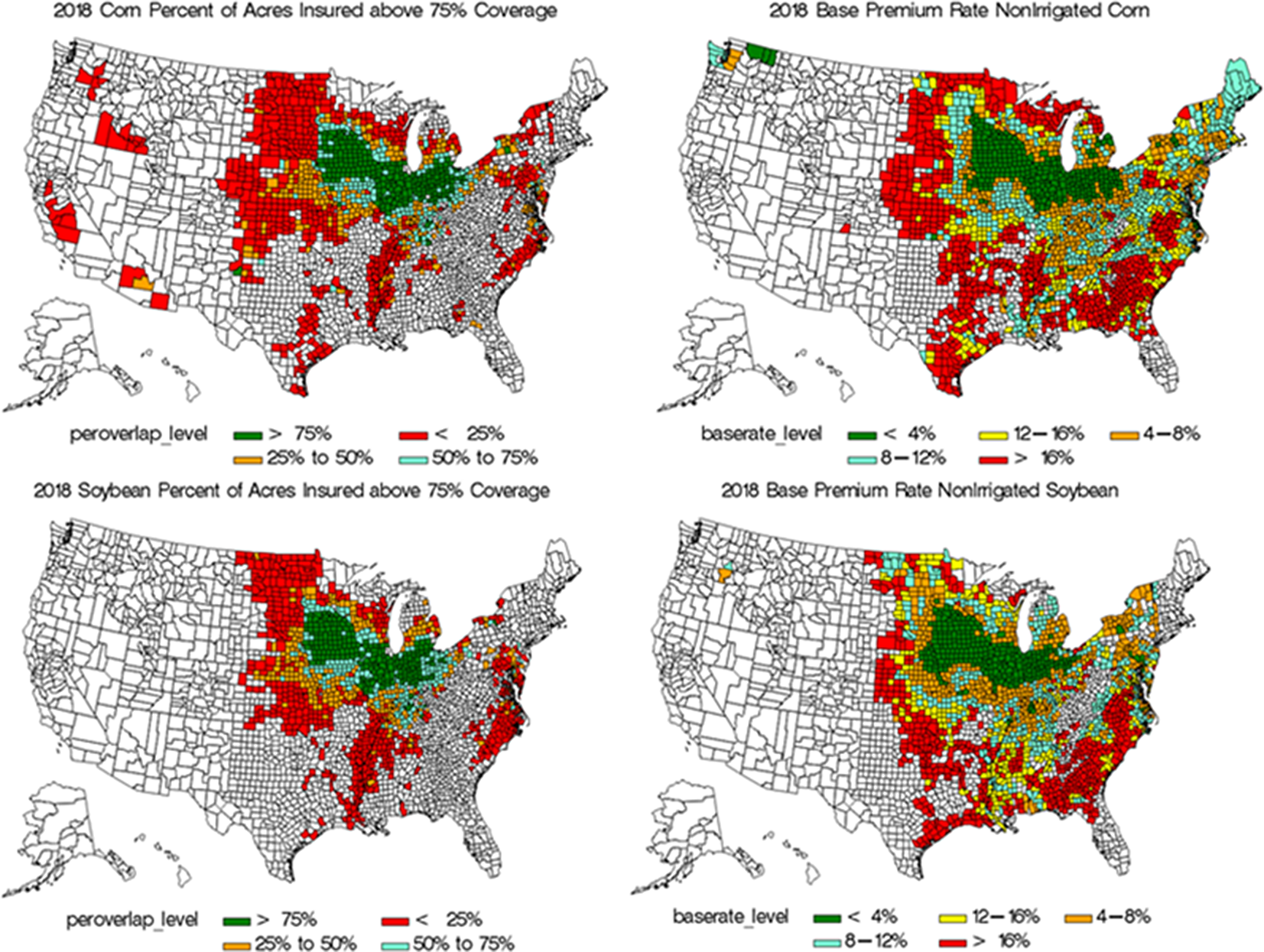
A history of RP coverage level enrollment since its introduction in 2011 shows that the 75% coverage level has been the most selected coverage level choice nationwide (Figure 3). In 2018, U.S. corn and soybean producers accounted for $2.6 billion in producer-paid premiums for RP insurance. Of this $2.6 billion, $1.2 billion (i.e., 44%) was associated with coverage levels that spanned the ARC coverage range. Furthermore, as will be established below, the additional producer-paid premium required for an increase in coverage (i.e., marginal premium) is greatest at coverage levels that are within the ARC coverage range. Another interesting aspect of RP purchase behavior is that producers in the relatively lower risk region of the Corn Belt opt for coverage levels within the ARC coverage range, while producers in relatively higher risk regions (e.g., the Mississippi Delta) do not; perhaps suggesting that this regionalFootnote 2 distinction could be driven by base premium rates (Figure 4). The correlation between RP enrollment within the ARC coverage range and county base premium rates for corn and soybeans are −0.58 and −0.64, respectively.
RP coverage level enrollment 2011–2018. Since the inception of Revenue Protection (RP), the most popular RP coverage level choice across all states on the average is 75%. Data source: RMA Summary of Business; rma.usda.gov.

Comparison between the 2018 percentage of RP-ARC overlap and base premium rates for corn and soybeans. Despite facing a lower probability of crop loss, counties in the Corn Belt enroll in higher coverage levels (i.e., 80–85%). This may be driven by the relatively lower base premium rates faced by producers in this region. Conversely, we see counties in the Mississippi Delta with less percentages enrolled in buy-up coverage, despite facing a higher likelihood of crop loss. Data source: RMA Summary of Business; rma.usda.gov.
While recent literature has addressed other shallow loss programs, such as STAX and SCO (Yehouenou et al., Reference Yehouenou, Barnett, Harri, Coble and McIntosh2018; Cooper, Hungerford, and O’Donoghue, Reference Cooper, Hungerford and O’Donoghue2015; Luitel, Hudson, and Knight, Reference Luitel, Hudson and Knight2018; Bulut and Collins, Reference Bulut and Collins2014), none have addressed the prima facie behavioral anomalies illustrated in this article. Bulut and Collins (Reference Bulut and Collins2014) find that commodity area plans are only a limited substitute for risk protection with individual insurance plans due to yield basis risk and generally have no impact on crop insurance choices. Yehouenou, Barnett, and Coble (Reference Yehouenou, Barnett, Harri, Coble and McIntosh2018) analyze the STAX program for cotton using the expected utility theory. The work presented by Yehouenou, Barnett, and Coble (Reference Yehouenou, Barnett, Harri, Coble and McIntosh2018) focuses on determining the optimal coverage level of STAX paired with RP, which are both crop insurance programs. Importantly, overlap of RP and STAX is not allowed. They find that a standalone STAX program would not be a very effective alternative to farm-level crop insurance and suggest that cotton producers in Texas would benefit more from using STAX as a complement to their farm-level crop insurance.
Cooper, Hungerford, and O’Donoghue (Reference Cooper, Hungerford and O’Donoghue2015) study the interactions of shallow loss support programs and traditional federal crop insurance programs. In their research, it is assumed that the producer already has acres enrolled in 75% coverage RP, and they are making the decision to sign up for ARC or SCO, both found under Title I in the 2014 farm bill. Cooper, Hungerford, and O’Donoghue (Reference Cooper, Hungerford and O’Donoghue2015) simulate revenue payments per acre with different farm program election combinations, rather than explore different levels of RP coverage to find the optimal level of coverage paired with ARC.
In addition to the work on the 2014 farm bill, there has been much work done on the potential for overlap in the 2008 farm bill (Heerman et al., Reference Heerman, Cooper, Johansson and Worth2016; Bulut, Collins, and Zacharias, Reference Bulut, Collins and Zacharias2012; Cooper and O’Donoghue, Reference Cooper and O’Donoghue2011; O’Donoghue et al., Reference O’Donoghue, Effland., Cooper and You2011; Cooper, Reference Cooper2010; Zulauf, Schnitkey, and Langemeier, Reference Zulauf, Schnitkey and Langemeier2010). Bulut, Collins, and Zacharias (Reference Bulut, Collins and Zacharias2012) examine the interaction between crop insurance and other farm support programs and are more concerned with how producers will react to farm policy proposals, rather than what has already been enacted into public law. Related to this work, Cooper and O’Donoghue (Reference Cooper and O’Donoghue2011) also explore whether receiving benefits from multiple programs affects producers’ business decisions by analyzing the overlap between 2008 farm bill crop insurance (SURE) and commodity (ACRE) programs, similar to their 2014 farm bill counterparts RP and ARC.
There has been little research on ARC in general (Orden and Zulauf, Reference Orden and Zulauf2015), and more specifically, previous research has not considered optimal RP coverage level choices in the presence of simultaneous enrollment in the ARC program. Here, we evaluate these decisions among producers in both the Corn Belt and Mississippi Delta under Expected Utility Theory using data from the USDA National Agricultural Statistics Service (NASS), the USDA Risk Management Agency (RMA), and the Commodity Research Bureau (CRB). Price and yield data are simulated using a Phoon, Quek, and Huang procedure (Phoon, Quek, and Huang, Reference Phoon, Quek and Huang2004). Focusing on a representative farm in McLean County (Illinois) and in Bolivar County (Mississippi) we find that optimal coverage level choices are (1) within the ARC coverage range and (2) higher in relatively less risky regions. McLean County is centrally located in the Corn Belt (i.e., Illinois, Indiana, and Iowa), and Bolivar County is centrally located in the Delta (i.e., Arkansas, Louisiana, Mississippi, Tennessee).
Conceptual Framework
Our approach follows a similar Expected Utility setup as Coble, Heifner, and Zuniga (Reference Coble, Heifner and Zuniga2000) in which the choice variable is the quantity of production hedge given that the producer is already insured. Under the Expected Utility framework, the base model represents a risk-averse producer choosing the optimal level of RP coverage to buy where the choice variable is the coverage level. Assuming the von Neumann-Morgenstern axioms of behavior, the producer maximizes their expected utility. The assumption that the producer is risk-averse rather than risk-neutral implies its utility function strictly increasing, concave, and twice continuously differentiable.
To explain the model, the utility function is broken down into equations for average crop revenues, RP indemnities, RP producer paid premiums, and ARC payments. Average crop revenues are found by the following equation:
 $$\tilde{R}_{i}=\tilde{P}^{{\rm Cash}}\tilde{Y}_{i}-C$$
where $\tilde R$
i
is the stochastic average crop revenue per planted acre for representative farm i,
$\tilde R$
i
is the stochastic average crop revenue per planted acre for representative farm i, $\tilde P$
Cash is the stochastic cash price received,
$\tilde P$
Cash is the stochastic cash price received, $\tilde Y$
i
is the stochastic farm-level yield for representative farm i, and C are total costs (in dollars) of production per acre, which differ by representative farm (see Table S6 in Online Appendix).
$\tilde Y$
i
is the stochastic farm-level yield for representative farm i, and C are total costs (in dollars) of production per acre, which differ by representative farm (see Table S6 in Online Appendix).
RP indemnities are calculated using the equation below:
 $$I_{i}={\rm MAX}\left\{\left[\left({\rm MAX}\left(F^{s},\tilde{F}\ \!^{f}\right)Y_{i}^{{\rm APH}}\phi \right)-\tilde{F}\ \!^{f}\tilde{Y}_{i}\right],0\right\}$$
where I
i
is the RP indemnity per planted acre for representative farm i, F
s
is the spring futures price, $\tilde F$
f
is the stochastic futures price in the fall, Y
i
APH is the APH (Actual Production History) yield for farm i, and
$\tilde F$
f
is the stochastic futures price in the fall, Y
i
APH is the APH (Actual Production History) yield for farm i, and $\phi$
is the RP coverage level chosen by the producer. RP producer paid premiums can be found with the following equation:
$\phi$
is the RP coverage level chosen by the producer. RP producer paid premiums can be found with the following equation:
 $$M_{i}=\phi F^{s}Y_{i}^{{\rm APH}}A_{i}\left(\phi \right)\left(1-S\left(\phi \right)\right)$$
where M i is the RP producer paid premium per planted acre for farm i, A i (ϕ) is the actuarially fair base premium rate, which is a function of the coverage level, faced by farm i, and S(ϕ) is the subsidy as a function of coverage level.
ARC payments are calculated using the equation below:
 $${\rm AR}{\rm C}_{i}=\left(0.85\right)A_{i}^{B}{\rm MIN}\left\{{\rm MAX}\left[\left(ZP^{O}Y_{C}^{O}-\tilde{P}^{{\rm MYA}}\tilde{Y}_{C}\right),0\right],0.1P^{O}Y_{C}^{O}\right\}$$
where ARC
i
is the total amount of ARC payment for farm i, A
i
B
is the number of base acres devoted to a specific commodity for farm i, P
O
is the Olympic Average price per bushel, Y
C
O
is the Olympic Average county yield for county C, $\tilde P$
MYA is the stochastic MYA (Marketing Year Average) price per bushel,
$\tilde P$
MYA is the stochastic MYA (Marketing Year Average) price per bushel, $\tilde Y$
C
is the stochastic county yield for county C, and Z is the ARC payment rate.Footnote
3
$\tilde Y$
C
is the stochastic county yield for county C, and Z is the ARC payment rate.Footnote
3
To model a producer deciding to choose an optimal RP coverage level, the above components (equations 1–4) are incorporated into an equation that forms the objective expected utility function below:
 $$\matrix{
{E\left( U \right) = \mathop {MAX}\limits_\phi \int_{{{\tilde P}^{{\rm{Cash}}}}} {\int_{{{\tilde P}^{{\rm{MYA}}}}} {\int_{{{\tilde F}^f}} {\int_{{{\tilde Y}_i}} {\int_{{{\tilde Y}_C}} U } } } } [A_i^P\left( {{{\tilde R}_i} + {I_i} - {M_i}} \right)} \hfill \cr
{\quad \quad \quad \quad + {\rm{AR}}{{\rm{C}}_i}]f\left( {{{\tilde P}^{{\rm{Cash}}}},{{\tilde P}^{{\rm{MYA}}}},{{\tilde F}^f},{{\tilde Y}_i},{{\tilde Y}_C}} \right)d{{\tilde P}^{{\rm{Cash}}}}d{{\tilde P}^{{\rm{MYA}}}}d{{\tilde F}^f}d{{\tilde Y}_i}d{{\tilde Y}_C}} \hfill \cr
} $$
$$\matrix{
{E\left( U \right) = \mathop {MAX}\limits_\phi \int_{{{\tilde P}^{{\rm{Cash}}}}} {\int_{{{\tilde P}^{{\rm{MYA}}}}} {\int_{{{\tilde F}^f}} {\int_{{{\tilde Y}_i}} {\int_{{{\tilde Y}_C}} U } } } } [A_i^P\left( {{{\tilde R}_i} + {I_i} - {M_i}} \right)} \hfill \cr
{\quad \quad \quad \quad + {\rm{AR}}{{\rm{C}}_i}]f\left( {{{\tilde P}^{{\rm{Cash}}}},{{\tilde P}^{{\rm{MYA}}}},{{\tilde F}^f},{{\tilde Y}_i},{{\tilde Y}_C}} \right)d{{\tilde P}^{{\rm{Cash}}}}d{{\tilde P}^{{\rm{MYA}}}}d{{\tilde F}^f}d{{\tilde Y}_i}d{{\tilde Y}_C}} \hfill \cr
} $$
where A i P is the total planted acres for farm i, and f(⋅) is a joint probability distribution of prices and yields.
Producers are assumed to maximize a constant relative risk aversion (CRRA) utility function:
 $$U={W^{1-\alpha } \over 1-\alpha} $$
where W is the initial wealth and α > 1 is a risk aversion parameter, which is set initially at α = 2.
For each scenario, the certainty equivalent (CE) calculated is given by:
 $${\rm CE}=\left[\left(1-\alpha \right)E\left(U\right)\right]^{1 \over 1-\alpha }$$
It is important to note that the CE is the dollar amount that would render the producer indifferent between receiving the dollar amount with certainty by using ARC and/or RP, or taking the gamble using no risk products. The largest CE indicates the optimal risk management choice between RP and ARC. Results were generated for scenarios with different combinations of RP coverage levels, premium structures (i.e., actuarially fair and subsidized), and the inclusion of ARC payments.
Price and Yield Stochastic Simulation
A joint distribution of yields and prices was simulated using a technique known as the Phoon, Quek, and Huang (PQH) procedure, as described by Phoon, Quek, and Huang (Reference Phoon, Quek and Huang2004) and applied in Anderson, Harri, and Coble (Reference Anderson, Harri and Coble2009). The reasons for choosing this sampling method are threefold. First, as implied by Anderson, Harri, and Coble (Reference Anderson, Harri and Coble2009) and pointed out by Woodard et al. (Reference Woodard, Paulson, Vedenov and Power2011), this method is the most similar to the Iman and Conover (IC) procedure (Iman and Conover, Reference Iman and Conover1982), which is the simulation procedure used by the RMA (Coble et al., Reference Coble, Knight, Goodwin, Miller, Rejesus and Duffield2010; Goodwin et al., Reference Goodwin, Harri, Rejesus, Coble and Knight2014). Second, the PQH is less computationally expensive and relatively more consistent than the IC (Anderson, Harri, and Coble, Reference Anderson, Harri and Coble2009). Third, in spite of a copulaFootnote 4 procedure’s flexibility and computational simplicity (Woodard et al., Reference Woodard, Paulson, Vedenov and Power2011; Ramsey, Goodwin, and Ghosh, Reference Ramsey, Goodwin and Ghosh2019), the PQH procedure calculates premium rates much closer to the true rates given by the RMA (see Tables S8 and S9 in Online Appendix). Nonetheless, it is important to consider whether results are sensitive to other sampling procedures. Therefore, we conduct a robustness check using a copula-based approach and find results follow a similar pattern. This is discussed in more detail in Appendix A.
For this work, farm and county yields were simulated by imposing a beta distribution, as presented by Nelson and Preckel (Reference Nelson and Preckel1989), as a distribution appropriate to model yield risk. County yields for corn and soybeans in McLean County, Illinois are for nonirrigated land, while those in Bolivar County, Mississippi are for irrigated land. Prices were simulated by imposing a lognormal distribution since prices often exhibit behavior consistent with lognormality (Goodwin and Ker, Reference Goodwin and Ker2002).
Each of the three prices used is simulated for each crop in the following way. We begin by creating a raw dataset of annual intraseasonal price movements in order to model the volatility of each price variable. Using the historical futures data, we calculate the change in the futures price from the planting month to the harvest month for a given crop. Then, we calculate an annual basis measure which is the difference in the futures price and the ending annual NASS state-level cash price received. Then, we do the same for the MYA price and calculate the annual basis between the futures price and the MYA price. Next, for each price in the sample, we create a sample of correlated probabilities of intraseasonal price movements drawn from a standard normal distribution using a probit function in SAS/IML, which are then used to calculate each random priceFootnote 5 variable.
December corn and November soybean futures price data from 1992 to 2017 are from the CRB. Final annual values for state-level cash prices received and the national MYA prices are taken from the NASS for the years 1992–2017. County yields used in the simulation come from RMA in the years 1992–2017. RMA county-level yields are used to calculate farm-level yields. To do this, we follow the COMBO rating process outlined in Coble et al. (Reference Coble, Knight, Goodwin, Miller, Rejesus and Duffield2010) by regressing county yields on time to obtain a linear time trend, which is then used to detrend county yieldsFootnote 6 in each county. The linear trend is found using the equation:
 $$Y_{Ct} = \beta_0 + \beta_{1*t} + \varepsilon_t$$
where Y Ct is the NASS-reported yield for county C in time t, β 0 is an intercept, β 1 is the linear trend coefficient to be estimated, and ϵ t is an error term. Using the linear trend found in equation (12), detrended farm-level yields were calculated using the equation below:
 $$Y_{it}=Y_{Ct}+\beta _{1}(2017-t)+\psi _{i}$$
where Y it is the yield for representative farm i in year t, and ψ is the idiosyncratic yield risk for representative farm i. In this work, we are only focused on two representative farms in each county—one that devotes all planted acres to corn and one that devotes all planted acres to soybeans. The idiosyncratic farm yield risk is a random number generated from a beta distribution with shape parameters that were endogenously determined given the RMA base premium rate. The standard deviation is the driver for the base premium rate calculation needed to calculate the producer paid premium and represents the amount of risk simulated by a representative farm yield that is different from the county yield. The larger the standard deviation is the riskier the farm is perceived to be, which in turn, generally results in higher base premium rates.
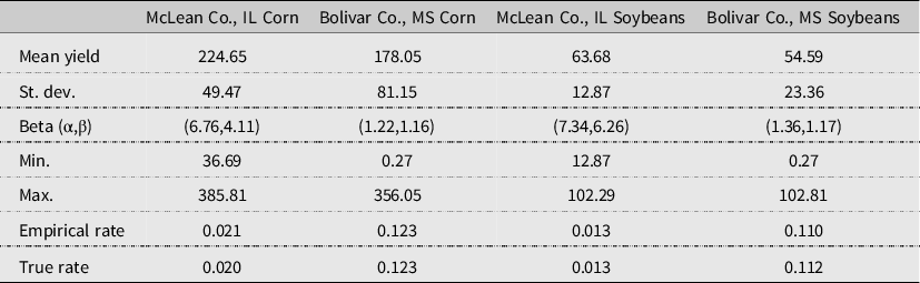
The specific procedure used to generate a sample of 25,000 yield observations at the farm-level incorporates both systemic variation at the county level and idiosyncratic variation at the farm level. First, we duplicate each of the 25 county-level de-trended yields 1000 times. Second, we assume values for the beta distribution parameters (α,β) such that the implied mean is the same as the mean of the county detrended yields. Note that for a given value of α, setting β = α(μ −1−1) will hold the mean of a beta distribution fixed. We assume the support for the beta distribution has a maximum at 1.5 times the largest observed county yield, and the minimum is set to insure a lower bound on yields of zero. Third, we draw from this distribution 25,000 times, demean those draws, add them to the detrended yields and calculate the empirical premium rate at the 75% coverage level. Steps 2 and 3 are repeated for all values of α between 0.5 and 10 in steps of 0.01. The final values of parameters are chosen as the ones for which the empirical rate is closest to the base premium rate. The characteristics of the farm-level samples of yields and the optimized values of the beta distribution are reported in Table 1.
Characteristics of farm-level yield samples
The empirical Pearson correlation coefficients used for the simulation, which are calculated using the sample consisting of historical county yields and prices from 1992 to 2017 and farm yields outlined above, for corn in both locations are given in Tables S1 and S2, while the empirical Pearson correlation matrices for soybeans in both locations are given in Tables S3 and S4. Summary statistics for county and farm yields, as well as the MYA, harvest, and cash pricesFootnote 7 for corn and soybeans in both locations, are given in Table S5.
Base premium rates for RP were calculated using the simulated yields and prices. There are two values needed to calculate a base premium rate for a given coverage level: total liability and the expected indemnity. The calculations required to arrive at a base premium rate for a given coverage level are given below. Total liability for a given coverage level is found using:
 $$L_{i}=\phi Y_{i}^{{\rm APH}}F^{S}$$
where L i is the total liability for farm i.
The revenue guarantee is calculated using the formula below:
 $$G_{i}=\phi Y_{i}^{{\rm APH}}{\rm MAX}\left(F^{S},P^{{\rm Cash}}\right)$$
where G i is the revenue guarantee.
The revenue guarantee is then used to calculate an indemnity, which we found in equation(2). Finally, the base premium rate for a given coverage level is calculated using the following formula:
 $$RP_{i}^{{\rm Base}\_ {\rm Rt}}={E\left(I_{i}\right) \over L_{i}}$$
Where RP i Base_Rt is the base premium rate, and E(I i ) is the expected value of the indemnity.
Exogenous Farm Program Parameters
Exogenous farm program parameters and on-farm costs are given in Table S6. The Olympic Average prices and yields required for the ARC payment guarantee are given, as well as a ratio of base to planted acres. On-farm per acre costs, as well as beginning futures prices for corn and soybeans for both locations, are also given. The OA yield was calculated from the real data used for the simulation of yields used to create the revenue distribution. We considered the last 5 years of RMA county yields, dropped the highest and lowest yields, then averaged the remaining three. The OA prices were also calculated from the data used for the simulated revenues and were calculated by taking the last 5 years of NASS cash prices received, dropping the highest and lowest prices, and averaging the remaining three prices. The loan rates are set by the USDA. The beginning futures prices, or the futures prices at planting, used were chosen based on USDA RMA’s price election amount in the liability calculation in the Cost Estimator. The on-farm costs per acre for McLean County, Illinois were taken from the 2018 crop budgets published by FarmDoc Daily. The on-farm costs per acre for Bolivar County, Mississippi were taken from the 2018 Mississippi State University Crop Irrigation Budgets published by the Mississippi State University Extension Service.
Scenarios for Risk Management
Four different scenarios were considered in determining the optimal RP coverage level for representative corn and soybean farms in McLean County, Illinois and Bolivar County, Mississippi. The first scenario (S1) consists of crop revenues and unsubsidized RP crop insurance and is the base case scenario for comparison to other scenarios that capture the influence of the subsidy and ARC on optimal coverage level choices. Scenario two (S2) consists of crop revenues and subsidized RP crop insurance and shows the effect of adding the subsidy to crop insurance. Importantly, by including the subsidy, the choice for the Illinois producer effectively differs from that of the Mississippi producer. Scenario three (S3) includes crop revenues, RP insurance, and ARC payments and is the scenario that reveals the optimal coverage level under the assumption that the producer has signed up for ARC and is deciding on which coverage level to sign up for. Essentially, each scenario adds complexity to the base case of unsubsidized insurance (S1). Under the current hypothesis, a representative producer in either region should choose a coverage level which does not extend into the ARC coverage range (i.e. 80% and 85%). Thus, under scenario three, once ARC is added across all coverage levels, the optimal coverage level should not be 80% or 85% if the hypothesis is correct.
Results
Simulated base premium rates for a farm in each county and for a given crop are given in Table S7. There is a significant difference in premium rates between the two locations under consideration. The rates follow the idea that farms in Illinois are less risky and have lower premium rates relative to farms in Mississippi. The relatively lower farm yields and relatively higher standard deviation in the Mississippi county are most likely the main drivers behind the relatively higher rates compared to Illinois. These higher premium rates could explain the low uptake in higher levels of RP insurance in the Mississippi Delta, while the lower premium rates in Illinois could explain the greater uptake in higher coverage levels as mentioned before. We investigate this further in Appendix B.
Optimal Risk Management Strategies Under EUT
Results for each of the three scenarios described above are presented here. Figure 5 and Figure 6 depict producer graphically decision-making within the model by location for corn. Results follow a similar pattern for soybeans.Footnote 8
McLean Co., IL Corn plotted certainty equivalents. The Scenarios here reflect the three outlined in the text: S1 (Unsubsidized Insurance); S2 (Subsidized Insurance); S3 (Subsidized Insurance + ARC).

Bolivar Co., MS Corn plotted certainty equivalents. The Scenarios here reflect the three outlined in the text: S1 (Unsubsidized Insurance); S2 (Subsidized Insurance); S3 (Subsidized Insurance + ARC).

Scenario 1: Unsubsidized Insurance
The CEs for both McLean County and Bolivar County under Scenario 1 are relatively flat compared to other scenarios (Figure 5 and Figure 6). This is most likely due to the nature of the relationship between the producer paid premium and the coverage level. With the subsidy set equal to zero, one reason for a producer to increase coverage levels would be if they perceive a greater amount of risk for their on-farm revenue, whether that be in yield risk or price risk. Lastly, with risk priced perfectly, we would expect a risk averse producer to choose the highest coverage level available.
Scenario 2: Subsidized Insurance Only
With the inclusion of the subsidy, the choice for the Illinois producer differs from that of the Mississippi producer (Figure 5 and Figure 6). Holding all others variables constant, it would appear that for both corn and soybeans the inclusion of the subsidy alters the decision for a producer in the higher-risk Bolivar County. Even though the optimal choice for a producer in McLean County remains at 85% for both corn and soybeans, the producer in Bolivar County lowers their optimal choice to 80% coverage. Furthermore, one can see by Figure 5 and Figure 6 that the slope of the CE’s experience a large increase relative to Scenario 1 further reinforcing the greater value of the subsidy (i.e., the difference between the CEs in Scenarios 1 and 2) to corn producers in Bolivar County versus that of those in McLean County. The value of the subsidy to a producer in Bolivar County is so great that the producer drops their chosen coverage level from 85% to 80%. In other words, the Bolivar County producer values the subsidy loss more than the increased risk reduction. Overall, it appears that a producer facing higher base premium rates will cause them to place a higher value on the subsidy compared to a producer facing relatively lower base premium rates.
For corn and soybean producers in McLean County, it would appear the CEs remain nearly the same between Scenarios 1 and 2 for 50–55% coverage in McLean County, and the value of the subsidy increases across all coverage levels (Figure 5 and Figure 6). Again, holding all other variables constant, the value of the subsidy is the greatest at the 85% coverage level, even though the subsidy percentage is the lowest at 85%. This might help explain the difference in the optimal choices in the two locations. A notably different value in the base premium rate may be causing McLean County producers to remain at 85% coverage, while the Bolivar County producers decreased their coverage choice to 80%.
Scenario 3: Subsidized Insurance with ARC
The inclusion of ARC as another added layer of risk protection produces noticeably different results. This introduces an important implication of the relationship between ARC and RP in terms of the enrollment decision. The plotted CE’s shift up in a parallel manner, implying that there is no direct relationship between the two programs. The case can be made here that ARC only shifts the plotted CEs by a value equivalent to that of an ARC payment. The reason for this could be because the revenue guarantee for ARC is calculated using historical county yields, while the revenue guarantee for RP is calculated using historical APH farm yields.
Another interesting finding within Scenario 3 is in the No Insurance choice. It is at this choice where one can make the distinction between ARC and RP as complements versus their effectiveness as standalone risk management programs. In the No Insurance choice, the producer has only enrolled in ARC and has chosen not to enroll in RP crop insurance. If only choosing ARC was the optimal risk management decision, it would have the highest CE. However, across locations and crops, the result remains the same: under Expected Utility, ARC is not an optimal standalone program in the presence of the option to enroll in RP. With the inclusion of RP insurance, the CE’s increase across both McLean County and Bolivar County, with Bolivar County remaining at the previous optimal choice of 80% RP coverage level.
As we have seen, regardless of if ARC is included in the RP enrollment decision, the Expected Utility-maximizing producer chooses to enroll in RP at a coverage level into the coverage range of ARC at either 80%, as in Bolivar County, or at 85%, as in McLean County.
Conclusions
Crop insurance and commodity programs are both effective approaches to risk management for producers. To create a way for these two to work in conjunction with one another, deep loss crop insurance and shallow loss commodity programs were created in the 2014 farm bill. Although the idea to stack shallow loss ARC on top of deep loss RP appeared to be one that could be effective, inefficiencies occurred. $2.5 billion of 2018 corn and soybean insurance liability overlapping with ARC cost producers out-of-pocket over $1 billion,Footnote 9 and more than half of that cost was explicitly for the overlapping coverage. Producers may have done this because they thought ARC would not cover them, so they signed up for RP to increase their chances of receiving a payment. The county-farm yield correlation may have been less than perfect and farm yields may not have been as high as county yields, so ARC may not have been the best option as a standalone risk management tool. This article attempts to answer the question of what the optimal coverage level of RP is paired with ARC under Expected Utility Theory.
Results indicate that it is optimal for a producer to choose a coverage level for revenue insurance that extends into the range of coverage provided by ARC; in other words, they choose to double cover rather than stack their coverages. Regardless of the location being considered here, the results show that a producer should double cover themselves or select an RP coverage level that is in the ARC coverage band of 76–86%. This is primarily driven by factors such as the changing subsidy rate schedule, risk aversion,Footnote 10 as well as the relative riskiness of each region indicated by base premium rates for RP insurance.
In McLean County, Illinois, 85% RP paired with ARC is the optimal combination, while 80% RP paired with ARC is the optimal combination for a producer in Bolivar County, Mississippi. Results are robust across sampling methods and other states in the regions considered (Appendices A and B). Using a copula-based approach, we find this did not alter the main finding of double coverage. One possible explanation for this is that the ARC-CO program in the 2014 farm bill did not differentiate yields based on irrigation practice. The 2018 farm bill differentiates yields by practice which could possibly reduce the double-coverage behavior since it may be associated with imperfect correlation between county and farm yields (i.e., yield basis risk) or the aggregation error between irrigated and non-irrigated yields. Further, given the 2018 farm bill’s decision mechanism allows for more flexibility in the ARC/PLC decision, the findings in this paper could impact the decision to enroll in RP coverage levels which span the ARC coverage range. A more nuanced and worthwhile extension of this work could include PLC in the decision-making process.
Another explanation for this optimal decision could be offered through a rule of thumb regarding the base premium rate (Appendix B). Bulut (Reference Bulut2017) provides interesting insight regarding the idea of a budget constraint driving regional heterogeneity in coverage level choices. We suggest a possible heuristic based on the crop and base premium rate and regardless of the location of the county. As we have noted previously, counties in which premium rates are relatively higher appear to result in a lower coverage level decision, so the question becomes what rate would push back the optimal coverage level. We find the premium rate threshold for corn to be 11%, while the premium rate for soybeans to be 10%. This avenue should be further explored in future work as it has implications for producers in counties in which they may not be choosing to buy-up into the higher coverage levels.
Supplementary material
For supplementary material accompanying this paper visit https://doi.org/10.1017/aae.2022.8
Data availability statement
The data that support the findings of this study are publicly available via the USDA National Agricultural Statistics Service Quick Stats portal and the USDA Risk Management Agency Summary of Business files. Additionally, some data have been acquired from the Commodity Research Bureau, which is now known as Barchart.com.
Acknowledgements
The authors would like to thank Olga Isengildina and three anonymous reviewers for their valuable comments and suggestions. Any remaining errors are our own.
Author contributions
Conceptualization, H.D.B. and K.H.C.; Methodology, H.D.B., K.H.C., A.H., J.T.; Formal Analysis, H.D.B., A.H., and J.T.; Data Curation, H.D.B. and A.H.; Writing— Original Draft, H.D.B.; Writing—Review and Editing, H.D.B., K.H.C., A.H., E.P., and J.T.; Supervision, H.D.B.; Funding Acquisition, K.H.C.
Funding statement
This work is supported by AFRI Project: Redesigning Farm Policy In An Era of Digital Agriculture Grant Number: 2017-06769/project accession no. 1015565 from the USDA National Institute of Food and Agriculture.
Competing interests
Keith Coble and Ardian Harri have done consulting work for the USDA Risk Management Agency which manages programs examined in this paper. However, the paper is not a product of that relationship. RMA has not had any input into this paper. Hunter Biram, Eunchun Park, and Jesse Tack declare no competing interests.
Appendix A: Results Under Copula Sampling Method
Using an empirical copula-based approach, results follow a similar pattern to that of the PQH approach (Figures S3-S6 in Online Appendix). In this alternative approach, the bounds and shape parameters for the yield distributions were chosen to match that of the bounds and shape parameters in the PQH approach. The key difference is the simulation of the probabilities associated with county and farm yields. Probabilities for all prices under the copula-based approach were simulated by assuming a standard normal distribution with mean zero and standard deviation of one. Further, under alternative dependency structures (i.e. Student’s t, Frank, and Clayton) results remained unchanged.
Additionally, the copula-based approach tended to over-calculate RMA RP base premium rates for corn relative to the PQH-based approach (Table S8). Rates calculated under both approaches for soybeans gave mixed outcomes, where the copula-based approach produced rates higher than that of the PQH-based approach (Table S9).
Appendix B: Spatial Heterogeneity in Coverage Level Choice
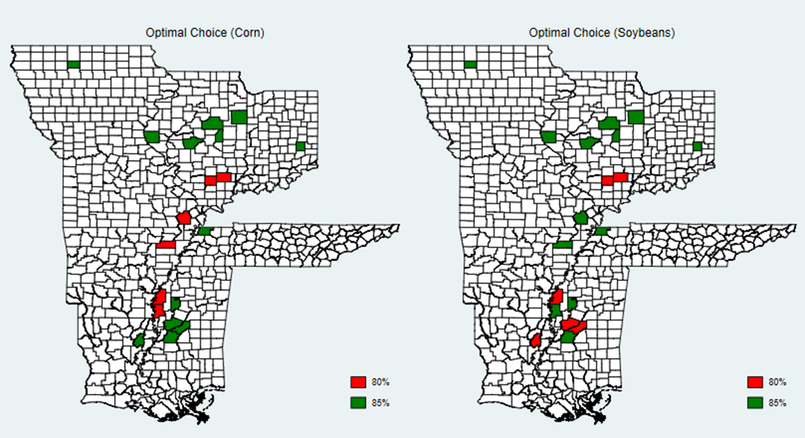
Upon adding counties which essentially have the same amount of acres in production and centrally span from the counties of interest, we show the main findings remain unchanged (Figure 1b). That is, in the presence of all eight coverage level options, the optimal RP coverage level choice remains 80% or 85%, both of which are in the ARC coverage range. Although there is some heterogeneity as to what the actual coverage level is (80 vs. 85%), all representative farmers in the counties considered would double cover.
Optimal Coverage Level Choice Heterogeneity. This map shows the spatial heterogeneity in optimal RP coverage level choices.
It appears there is a possible heuristic (Bulut, Reference Bulut2017), or rule of thumb, driving this regional heterogeneity (Figure 2b). Once the premium rate for RP corn is above 11%, it becomes optimal for a representative producer to enroll in a lower coverage level. For RP soybeans, the decision rule appears to be the same for a premium rate of 10%. We do not view this relationship between the coverage level and premium rate as a conclusive finding, but rather an interesting connection that future research may consider flushing out more definitively.
The Relationship Between Optimal Coverage Levels and Premium Rates. The scatter plots above of optimal coverage levels on their respective base premium rates exhibit a sharp discontinuity at their respective decision rules.


 Open access