


Introduction
The spatial clusters favorable to crop cultivation form the centers of agrarian intensification and economic development (Zabel et al. Reference Zabel, Delzeit, Schneider, Seppelt, Mauser and Václavík2019; Zimmerer Reference Zimmerer2013). Agriculture, as a spatial industry (Marasteanu and Jaenicke Reference Marasteanu and Jaenicke2016), the disparities in regional crop yields are shaped by variations in weather patterns and the application of agricultural inputs, as demonstrated by the work of Niyogi et al. (Reference Niyogi, Kishtawal, Tripathi and Govindaraju2010) and Sesmero et al. (Reference Sesmero, Ricker-Gilbert and Cook2018). Farm management decisions are influenced by the adoption of technology and the flow of information within and between regions (Gupta et al. Reference Gupta, Ponticelli and Tesei2024; Krishnan and Patnam Reference Krishnan and Patnam2014; Maertens Reference Maertens2017). These factors are integral in understanding the dynamics of spatial agricultural clusters and their impact on productivity and economic growth (Binswanger-Mkhize and Savastano Reference Binswanger-Mkhize and Savastano2017; Foster and Rosenzweig Reference Foster and Rosenzweig1995). In addition to agroclimatic factors, cropping practices, and regional agricultural policies, knowledge networks influence the crop yields (Gupta et al. Reference Gupta, Ponticelli and Tesei2024). Yield gaps across regions are a major concern in developing countries, particularly in India and African countries, due to multiple factors (Das Reference Das2006; Tian and Yu Reference Tian and Yu2019).
Crop yields in India are influenced by seasons. In our analysis, we examine the spatial distribution of seasonal yields for the major food grains in India from 2010 to 2019: paddy, wheat, and millets (i.e., the millets group, comprising Sorghum, Pearl millet, Finger millet, and Little millet (Gowri and Shivakumar Reference Gowri and Shivakumar2020; Nagaraj et al. Reference Nagaraj, Basavaraj, Rao, Bantilan and Haldar2013)). The spatial distribution of crop yield district clusters varies with crops and seasons. Since crop yield hotspots are economically desirable,Footnote 1 policymakers will be interested in the locations of high- and low-performing crop yield district clusters. The factors influencing these district cluster formations will provide actionable insights. Our analysis answers the following questions: What are the locations of district-level seasonal crop yield hot/coldspot clustersFootnote 2 in India? How do weather and input factors influence these cluster formations?
We hypothesize that crop yield hotspot clusters are located in high-input-intensive cropping systems. The analysis incorporates an evaluation of the spatial and temporal patterns of crop yield hotspots and coldspots, comparing these distributions with weather variables – particularly rainfall patterns and rainfall deviations from historical norms – as well as with factors such as irrigation coverage, fertilizer usage, and the incidences of agricultural information demand (or queries) at the farmers’ (Kisan) call centers (KCC). Weather and input factors are crucial for Indian agriculture (Goyari Reference Goyari2014; Kalirajan Reference Kalirajan1981; Letta et al. Reference Letta, Montalbano and Pierre2022).
Our evaluation reveals that the average yield differences between districts designated as ”hotspot” and those designated as ”coldspot” for paddy, wheat, and millets are 2, 2.4, and 1 t ha−1, respectively. Overall, high-yielding crop yield clusters are in the northern districts of Punjab and Haryana and in the southern districts of Telangana, Andhra Pradesh, Karnataka, and Tamil Nadu. Madhya Pradesh, located in the central region, aspires to be a hotspot cluster for all three food grains. The optimized use of input factors, synchronized with weather data and bolstered by information from the KCC, is a contributing factor to the emergence of these hotspot clusters in India. The results of the fixed-effect regression models studying the relationships between crop yield and these factors (Dayal Reference Dayal1984) substantiate this assertion. For instance, districts in Bihar, eastern India, despite their higher use of inputs such as irrigation and fertilizers, exhibit limited engagement with KCC regarding access to crop-specific information, resulting in their continued categorization as crop-yield low-performance clusters throughout the study period. However, through the strategic application of irrigation and fertilizers and the use of information resources in tandem, districts in Madhya Pradesh and Odisha have achieved notable improvements in crop yield performance over the study period. Crop yield coldspot districts need to double their yield performance to become hotspots. In Darbhanga district, Bihar, closing the hotspot–coldspot yield gap could raise household revenue by up to 148% for paddy and 79% for wheat.
Our analysis emphasizes the importance of the identification of hot/coldspots or high/low-yielding districts and characterizes the inherent differences in cropping practices besides the agro-climatic locations of these clusters. It is inferred that information, a crucial input in agriculture, yields improved regional productivity when utilized judiciously in conjunction with other input factors. This scale and in-depth analysis of production variability for major food grains at the district level in India is a unique contribution to the existing literature and provides actionable insights to policymakers.
The remainder of the paper is organized as follows. The Section (Literature review and empirical methodology) provides an overview of related literature and empirical methodology, and Section (Data) illustrates the data used in the analysis. The Section (Results and Discussions) summarizes the results and discusses the findings, Section (Robustness Checks) presents robustness checks of the empirical analysis of the hotspots, and Section (Conclusion) concludes the paper.
Literature review and empirical methodology
In this section, we present a brief literature review on yield gaps and hotspot methodology and position our research within this context. Subsequently, we discuss our empirical strategy for identifying crop yield hot/coldspot clusters and the factors that drive their formation.
Related literature on yield gaps and hotspot identification
India, being a subcontinent, has a diverse agricultural economy. The analysis of India’s agrarian data presents generalizable and policy-relevant insights for other developing countries (Fabregas et al. Reference Fabregas, Harigaya, Kremer and Ramrattan2022). The literature indicates that Southeast Asian and sub-Saharan African countries need to increase grain yields to meet their food security needs and reduce the reliance on food grain imports. Pasuquin et al. (Reference Pasuquin, Pampolino, Witt, Dobermann, Oberthür, Fisher and Inubushi2014)’s analysis on field trial data on maize concludes efficient use of nitrogen reduces farm productivity and profitability in Indonesia, the Philippines, and Vietnam. Another study on Southeast Asia by (Yuan et al. Reference Yuan, Stuart, Laborte, Rattalino Edreira, Dobermann, Kien, Thúy, Paothong, Traesang, Tint, San, Villafuerte, Quicho, Pame, Then, Flor, Thon, Agus, Agustiani, Deng, Li and Grassini2022) reports that yield gaps vary substantially across national and regional levels in rice production, with an average yield gap of 48%. India, as a frontier agrarian economy among South and Southeast Asian countries, can not only drive regional growth by improving its own crop yields but also share technological know-how with other regional economies (Liu et al. Reference Liu, Wang, Yang, Rahman and Sriboonchitta2020). While in sub-Saharan Africa, low crop yields need to be addressed through crop intensification and efficient agricultural extension systems (Corbeels et al. Reference Corbeels, Naudin, Whitbread, Kühne and Letourmy2020; Jayne and Sanchez Reference Jayne and Sanchez2021). The inference from the India-level hotspot analysis on major food grains applies to other developing countries in Southeast Asia and sub-Saharan Africa. The relationships between weather factors, inputs, and crop yields can serve as a baseline for these geographies, especially where high-quality data are scarce.
Hotspot analysis illuminates spatial variations of a variable of interest and identifies high-performing or risk-prone zones. In general, spatial studies identifying hotspots use spatial statistics such as Local Moran’s I, following geographic information system (GIS) applications. For instance, Shackelford et al. (Reference Shackelford, Steward, German, Sait, Benton and Richardson2015) used hotspot analysis to identify conservation conflicts in agricultural landscapes at the country level, and Marasteanu and Jaenicke (Reference Marasteanu and Jaenicke2019) identified organic agriculture hotspots using United States county-level data. But these techniques lack a temporal scale of measurement. Besides agriculture and environmental studies (Asseng et al. Reference Asseng, Cammarano, Basso, Chung, Alderman, Sonder, Reynolds and Lobell2017; Karimi et al. Reference Karimi, Brown and Hockings2015), hotspot analysis techniques are used to detect crime and traffic accidents (Mohler et al. Reference Mohler, Porter, Carter and LaFree2020). Along with spatial statistical analysis, socio-economic studies have used mathematical models to rank high-frequency events at both spatial and temporal scales Cheng and Washington (Reference Cheng and Washington2008); Gao et al. (Reference Gao, Zhang, Wang, Fu, Li, Dong, Yuan, Li and Jiao2024).
Our analysis involves both spatial and temporal dimensions, coupled with a ranking technique and a statistical significance test to identify district clusters or zones with sustained high productivity or significant positive changes. Quantitative studies such as those by Van Wart et al. (Reference van Wart, van Bussel, Wolf, Licker, Grassini, Nelson, Boogaard, Gerber, Mueller, Claessens, van Ittersum and Cassman2013) and others have applied similar methodology in zoning, yield gap analysis, and hotspot identification for policy and resource allocation. In addition to identifying hotspot districts, we identify coldspots and low-performing district clusters by tracking changes in crop yields over time. Our simplistic methodology for identifying hot/coldspots is based on district-level observed temporal data. These are the distinguishing characteristics of our methodology compared to existing hotspot analyses in the literature. Furthermore, we provide causal traction in our analysis by including weather and input factors that influence crop yield differences and verify the crop yield hot/coldspot distributions.
Hotspot identification
The approach for identifying districts with high crop yield potential, known as hotspots, uses a comprehensive two-step methodology. Initially, districts are designated as hotspots if their crop yield performances are equal to or exceed the 80th percentile rankFootnote 3 in any evaluated timeframe (Period 1: 2010–14 or Period 2: 2015–19). Moreover, districts exhibiting statistically significant increases in crop yields relative to national averages from Period 1 to Period 2 are also categorized as hotspots. Districts that have historically achieved high yields have likely met or surpassed the upper yield thresholds, thus presenting limited room for further substantive yield improvements. Consequently, for a district to be recognized as a hotspot in terms of seasonal crop yield, it must meet either of these two specific criteria. On the other hand, districts that display significant negative crop yield differences compared to national averages from Period 1 to Period 2 are designated as coldspots.
The estimation equation for the average seasonal crop yield, relative to the respective national averages, is given in equation (1), and the statistical significance of the yield differences is assessed using a two-sample Student’s t-test, following equation (2). ${\overline {YieldDiff} _{(ds)crp}} = {1 \over 5}\sum\limits_{{y_{{p_i} = 1}}}^5 {\left(Yiel{d_{(ds)cr{y_{{p_i}}}}} - {1 \over {5 \cdot n}}\sum\limits_{{y_{{p_i} = 1}}}^5 {\sum\limits_{(ds) = 1}^n Y } iel{d_{(ds)cr{y_{{p_i}}}}}\right)}$
where, $\overline {YieldDiff}$
: Average yield difference, (ds): District-State, n: Total number of districts (732), c: crops (i.e., paddy, wheat and millets) r: Seasons, p
i
: i
th
period (i=1,2) and y: Year sequence in a period (p
i
).
$\overline {YieldDiff}$
: Average yield difference, (ds): District-State, n: Total number of districts (732), c: crops (i.e., paddy, wheat and millets) r: Seasons, p
i
: i
th
period (i=1,2) and y: Year sequence in a period (p
i
).
Student’s two-sample t-test: The test to compare district-level yield differences between periods p 1 (2010–2014) and p 2 (2015–2019) based on seasonal crop yield averages. The standard t-test formulae are illustrated in our context as follows: ${t_{(ds)cr}} = {{{{\overline {YieldDiff} }_{(ds)cr{p_1}}} - {{\overline {YieldDiff} }_{(ds)cr{p_2}}}} \over {\sqrt {s_{(ds)cr}^2\left({1 \over {{m_1}}} + {1 \over {{m_2}}}\right)} }}$ $\small {s_{(ds)cr}^2 = {{\sum\nolimits_{i = 1}^{{m_1}} {{{\left(YieldDif{f_{(ds)cr{p_1}}} - {{\overline {YieldDiff} }_{(ds)cr{p_1}}}\right)}^2}} + \sum\nolimits_{j = 1}^{{m_2}} {{{\left(YieldDif{f_{(ds)cr{p_2}}} - {{\overline {YieldDiff} }_{(ds)cr{p_2}}}\right)}^2}} } \over {{m_1} + {m_2} - 2}}}$
where, t: Student’s t-statistic, s: standard deviation, m i : number of observations for crop yields in respective districts and corresponding period (p i ).
Yield volatility, input efficiency, and total factor productivity (TFP) provide complementary insights but also pose challenges in data availability, consistency, and interpretability at the district scale and for long-term trend assessments. Volatility, for instance, may highlight risk-prone districts but does not directly capture persistent or above-average productivity. TFP and input efficiency require detailed, reliable data on inputs, labor, and capital, which are often unavailable or inconsistent at the district level in India.
This classification approach is limited by its reliance on average yields, which may miss districts with high productivity but also high risk (volatility). Similarly, districts achieving efficiency gains or TFP improvements without large yield changes may be undervalued. The literature cautions that using a single metric risks omitting multi-faceted agro-ecological or socio-economic dynamics and that hotspot definitions should be complemented with additional criteria where possible (Pironon et al. Reference Pironon, Borrell, Ondo, Douglas, Phillips, Khoury, Kantar, Fumia, Soto Gomez, Viruel, Govaerts, Forest and Antonelli2020). Thus, we explored other available factors contributing to the yields and explored their relationships.
We follow similar crop yield hotspot/coldspot identification techniques to identify the influencing factors contributing to crop yields at the district level. These factors include observed rainfall, deviations in rainfall, crop-specific percentage of gross irrigated area, fertilizer consumption per gross cropped area, and the percentage of district-level KCC queries for the selected crops by season. These additional hotspot maps for rainfall and input factors are used to compare the distribution of the crop yield clusters. Since weather plays a vital role in the evolution of cropping systems and in differences in crop yields, we map aggregated weather deviations (maximum temperature, minimum temperature, and rainfall) to better infer crop yield differences. The empirical techniques for weather deviations are in the following subsection.
Weather deviations
Weather is an important factor contributing to the yield differences. We measure weather deviations for three variables relative to historical averages. The variables of weather deviation designed for analysis include the minimum temperature deviation (minTD (ds)ry ), maximum temperature deviation (maxTD (ds)ry ), and rainfall deviation (RD (ds)ry ). The following equations are used to measure weather deviations. $maxT{D_{(ds)ry}} = \left\{ {\matrix{ 0 & {{\rm{if}}\;{1 \over n}\sum\nolimits_{n = 2000}^{2019} m ax{T_{(ds)r}} - 2\sigma max{T_{(ds)r}} \le max{T_{(ds)ry}}} \cr {} & \!\!\!\!\!\!\!\!\!\!\!\!\!\!\!\!\!\!\!\!\!\!\!\!\!\!\!\!\!\!{ \le {1 \over n}\sum\nolimits_{n = 2000}^{2019} m ax{T_{(ds)r}} + 2\sigma max{T_{(ds)r}},} \cr 1 & \!\!\!\!\!\!\!\!\!\!\!\!\!\!\!\!\!\!\!\!\!\!\!\!\!\!\!\!\!\!\!\!\!\!\!\!\!\!\!\!\!\!\!\!\!\!\!\!\!\!\!\!\!\!\!\!\!\!\!\!\!\!\!\!\!\!\!\!\!\!\!\!\!\!\!\!\!\!\!\!\!\!\!\!\!\!\!\!\!\!\!\!\!\!{{\rm{otherwise}}.} \cr } } \right.$ $minT{D_{(ds)ry}} = \left\{ {\matrix{ 0 & {{\rm{if}}\;{1 \over n}\sum\nolimits_{n = 2000}^{2019} m in{T_{(ds)r}} - 2\sigma min{T_{(ds)r}} \le min{T_{(ds)ry}}} \cr {} & \!\!\!\!\!\!\!\!\!\!\!\!\!\!\!\!\!\!\!\!\!\!\!\!\!\!\!\!\!{ \le {1 \over n}\sum\nolimits_{n = 2000}^{2019} m in{T_{(ds)r}} + 2\sigma min{T_{(ds)r}},} \cr 1 & \!\!\!\!\!\!\!\!\!\!\!\!\!\!\!\!\!\!\!\!\!\!\!\!\!\!\!\!\!\!\!\!\!\!\!\!\!\!\!\!\!\!\!\!\!\!\!\!\!\!\!\!\!\!\!\!\!\!\!\!\!\!\!\!\!\!\!\!\!\!\!\!\!\!\!\!\!\!\!\!\!\!\!\!\!\!\!\!\!\!\!\!{{\rm{otherwise}}.} \cr } } \right.$ $R{D_{(ds)ry}} = \left\{ {\matrix{ 0 & {{\rm{if}}\;{1 \over n}\sum\nolimits_{n = 2000}^{2019} {{R_{(ds)r}}} - 2\sigma {R_{(ds)r}} \le {R_{(ds)ry}}} \cr {} & \!\!\!\!\!\!\!\!\!\!\!\!\!\!\!\!\!\!\!\!\!{ \le {1 \over n}\sum\nolimits_{n = 2000}^{2019} {{R_{(ds)r}}} + 2\sigma {R_{(ds)r}},} \cr 1 & \!\!\!\!\!\!\!\!\!\!\!\!\!\!\!\!\!\!\!\!\!\!\!\!\!\!\!\!\!\!\!\!\!\!\!\!\!\!\!\!\!\!\!\!\!\!\!\!\!\!\!\!\!\!\!\!\!\!\!\!\!\!\!\!\!\!\!{{\rm{otherwise}}.} \cr } } \right.$
where, σ(maxT (ds)r ), σ(minT (ds)r ), and σ(R (ds)r ) denote the standard deviations of minimum temperature, maximum temperature, and rainfall, respectively.
The variations in individual weather parameters across districts are aggregated to obtain an average z-score for each district. These aggregated district-level z-scores are compared with crop yield hot/coldspots. A positive z-score indicates notable historical deviations in the weather parameters, and vice versa. The z-score formula utilized in our study is presented below. ${\overline {z - ScoreWD} _{(ds)}} = {1 \over 3}\sum\limits_{w = 1}^3 {{{W{D_{(ds)w}} - \mu W{D_{(ds)w}}} \over {\sigma W{D_{(ds)w}}}}}$
where, (ds) is district-State observation, r denotes season, w represents weather variables (maximum temperature, minimum temperature, and rainfall), WD denotes the number of deviations for each weather variable for each district, μWD is the mean of weather deviation comprising all the districts, and σWD represents the standard deviation of weather deviation comprising all the districts.
Model determining factors influencing crop yield hotspots
Subsequently, we conduct a detailed empirical analysis to elucidate the determinants of the emergence of hotspots or positive yield deviations. We explore these relationships using a fixed-effect regression model. Rainfall is considered a vital biophysical factor among weather variables. First, we evaluate the relationships between the percentage of the gross irrigated area (GIA) and both observed rainfall and rainfall deviations (RD). Following this, we investigate the relationship between seasonal crop yield deviations and a set of influencing factors, including weather factors (observed and deviations), irrigation coverage, crop-specific KCC queries, and fertilizer consumption. $\eqalign{ & {{\boldsymbol GIA}_{(ds)cp}} = {\boldsymbol\alpha} + {\boldsymbol\beta _1Rai{n}_{(ds)rp}} + {\boldsymbol\beta _2R{D}_{(ds)rp}} \cr & \ \ \ \ \ \ \ \ \ \ + {{\boldsymbol\lambda} _a} + {{\boldsymbol\eta} _{(ds)}} + {{\boldsymbol\psi} _r} + {{\boldsymbol\eta} _{(ds)}} \times {{\boldsymbol\psi} _r} + {{\boldsymbol\omega} _c} + {{\boldsymbol\phi} _p} + {{\boldsymbol\varepsilon} _{a(ds)cp}} \cr}$ $\small{\eqalign{ & {\boldsymbol YieldDif{f}_{(ds)crp}} = {\boldsymbol\alpha} + {{\boldsymbol\beta _1Rai{n}}_{(ds)rp}} + {{\boldsymbol\beta _2R{D}}_{(ds)rp}} + {{\boldsymbol\beta _3GI{A}}_{(ds)cp}} + {{\boldsymbol\beta _4NP{K}}_{(ds)p}} + {{\boldsymbol\beta _5Querie{s}}_{(ds)crp}} \cr & \ \ \ \ \ \ \ \ \ \ \ \ \ \ \ \ \ + {{\boldsymbol\gamma _1{X}}_{(ds)rp}} + {{\boldsymbol\gamma _2{Y}}_{(ds)rp}} + {{\boldsymbol\lambda} _a} + {{\boldsymbol\eta} _{(ds)}} + {{\boldsymbol\psi} _r} + {{\boldsymbol\eta} _{(ds)}} \times {{\boldsymbol\psi} _r} + {{\boldsymbol\omega} _c} + {{\boldsymbol\phi} _p} + {{\boldsymbol\varepsilon} _{a(ds)crp}} \cr}}$
In equation 4, GIA (ds)cp represents the average percentage gross irrigated area in d, State s, crop c, and period p. The coefficients β 1 and β 2 capture the effect of changes in the percentage gross irrigated area related to average rainfall and total rainfall deviations.
Next, in equation 5, Yield (ds)crp (t ha−1) represents the seasonal yields of paddy in district d, State s, crop c, season r and period p. The coefficients β 1, β 2, β 3, β 4 and β 5, capture the effect of changes in the average rainfall (mm.), total rainfall deviation (i.e., dummy variable, 0 or 1), gross irrigated area (%), fertilizer consumptions (kg ha−1) and district-level queries related to specific crops and seasons at KCC (%).
The variable X( ds)ry is a vector of other observed weather controls that capture average maximum and minimum temperatures (∘C) in the districts. The variable Y( ds)ry is a vector of other weather deviation controls for the district’s maximum and minimum temperatures (i.e., dummy variables, 0 or 1). In both the regression equations above, the fixed effects of the region (λ a ), district-State (η( ds) ), season (ψ r ), crop (ω c ), and period (φ p ) are included in the analysis to account for the unobserved heterogeneity at these levels. These fixed effects are implemented as sets of indicator (dummy) variables. No observation weights are applied, and estimation proceeds without further transformations such as a within estimator. These categorical fixed effects absorb all time-invariant heterogeneity across regions, district-State, season, crop types, and periods. Consequently, any additional regressor constant within these dimensions (e.g., time-invariant soil characteristics varying only by district-State and region) is perfectly collinear with the dummies, automatically excluded from identification, and not reported in the results. Standard errors are clustered at the state-district level to address the potential correlation within the same district-State.
Data
In our empirical study, we draw on multiple district-level data sources from 2010 to 2019. First, we extract data on seasonal crop yields and gross cropped area for paddy, wheat, and millets. Second, we collect crop-specific and gross irrigated area data, as well as total fertilizer consumption data. These datasets are sourced from the government databaseFootnote 4 as well as the International Crops Research Institute for the Semi-Arid Tropics (ICRISAT) district-level database.Footnote 5 Third, we obtain twenty years’ (2000 to 2019) of monthly climatological observations from the TerraClimateFootnote 6 database, which are used in quantifying seasonal weather variations throughout the study duration of 2010 to 2019. Fourth, our analysis involves data collated from farmers’ (Kisan) call centers (KCC), a digital agriculture service provided by the government.Footnote 7 This dataset provides insights into the reach and efficacy of agricultural extension services via mobile phones, particularly for crops such as paddy, wheat, and millets, across all districts in India. We conducted an extensive analysis of farmers’ conversations using text-analysis protocols and developed an agricultural data dictionary to classify the conversations into three crop types (i.e., three dummy variables per crop).
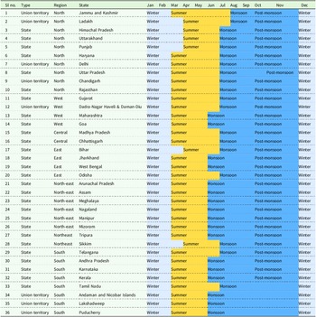
Indian crop production follows a seasonal cropping pattern aligned with monsoon rains (the Kharif season), winter (the Rabi season), and summer. The monthly distribution of these cropping seasons varies according to agroclimatic regions, geographic regions, and States (Figure 1 and Table 1). Typically, the monsoon season begins in July or August and lasts until October or November. Winter spans three months from December to February, while summer generally commences in March or April and continues until June or July.
Map of agroclimatic zones in India.
State and Union territory-wise monthly distribution of seasons
Note: The mapping of seasons with respect to the month and the administrative regions is based on information from the government and other reliable websites of each State and Union territory.
While analyzing the seasonal crop yield data, we divide it into two consecutive five-year periods for comparative analysis. The first period (2010–2014), with the start year matching the 2010–11 agricultural census. The second period covers 2015–2019, beginning with the 2015–16 agricultural census year. Comparing district-level yields between these two periods allows us to assess yield changes over time, indicating hot/coldspots.
On the other hand, we have weather data from 2000 to 2019, including average monthly minimum and maximum temperatures and total monthly rainfall. The seasonal weather deviations are estimated for each district for the period (2010 to 2019). In addition to weather data, we have the average percentage of gross irrigated area by crop type, as well as the average percentage of seasonal KCC queries for each crop type and district over the study period. We integrate these datasets, along with the fertilizer dataset, by crop, season, and period for our empirical analysis. We compare the influence of these agro-climatic factors on the formation of crop yield hotspots or coldspots across the country. We hypothesize that the distributions of input consumptions (i.e., irrigation, fertilizer consumption, and information access through KCC) have positive effects on hotspot cluster formation. In contrast, weather deviations (in particular, rainfall deviations) negatively affect the formation of positive yield deviations or hotspot clusters.
Results and discussions
We present maps of district-level crop yield differences that illustrate the seasonal cropping patterns of the regions, along with the identification of hotspot and coldspot clusters for each crop in each season. On the other hand, maps of weather deviations, the percentage of gross-irrigated area, fertilizer consumption, and access to crop-specific information via mobile phones from KCC highlight the biophysical and informational factors (or inputs) that influence crop yields. We hypothesize that crop yield hotspots will be in districts with the least deviations from the weather and the highest input consumptions. We explore the relationships between crop yield and these factors using hotspot maps and fixed-effect models in the following subsections.
Analysis of district-level crop yield differences and hotspots
We identify the crop yield hot/cold spots of the respective seasons in a two-step procedure as described in the Section 2 and discuss the results in detail in this subsection. For a broader view of the seasonal crop yield performances, the regional leaders are south for paddy, north for wheat, and south for millets (Table 2).
Region and season-wise paddy, wheat, and millets yields (2010–2019)
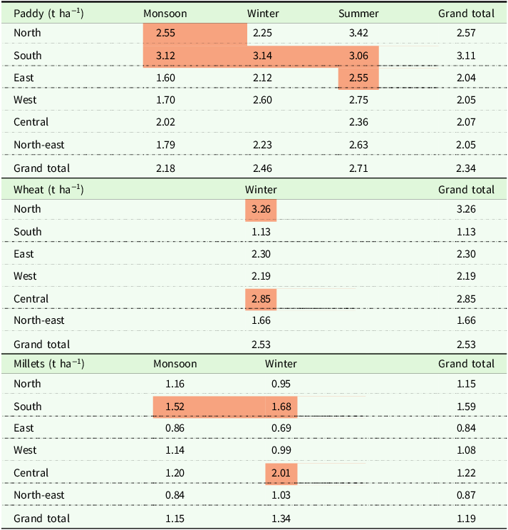
Note: The high-yielding regions are highlighted, considering crop yield performances and reasonable acreage of the crops in the respective regions.
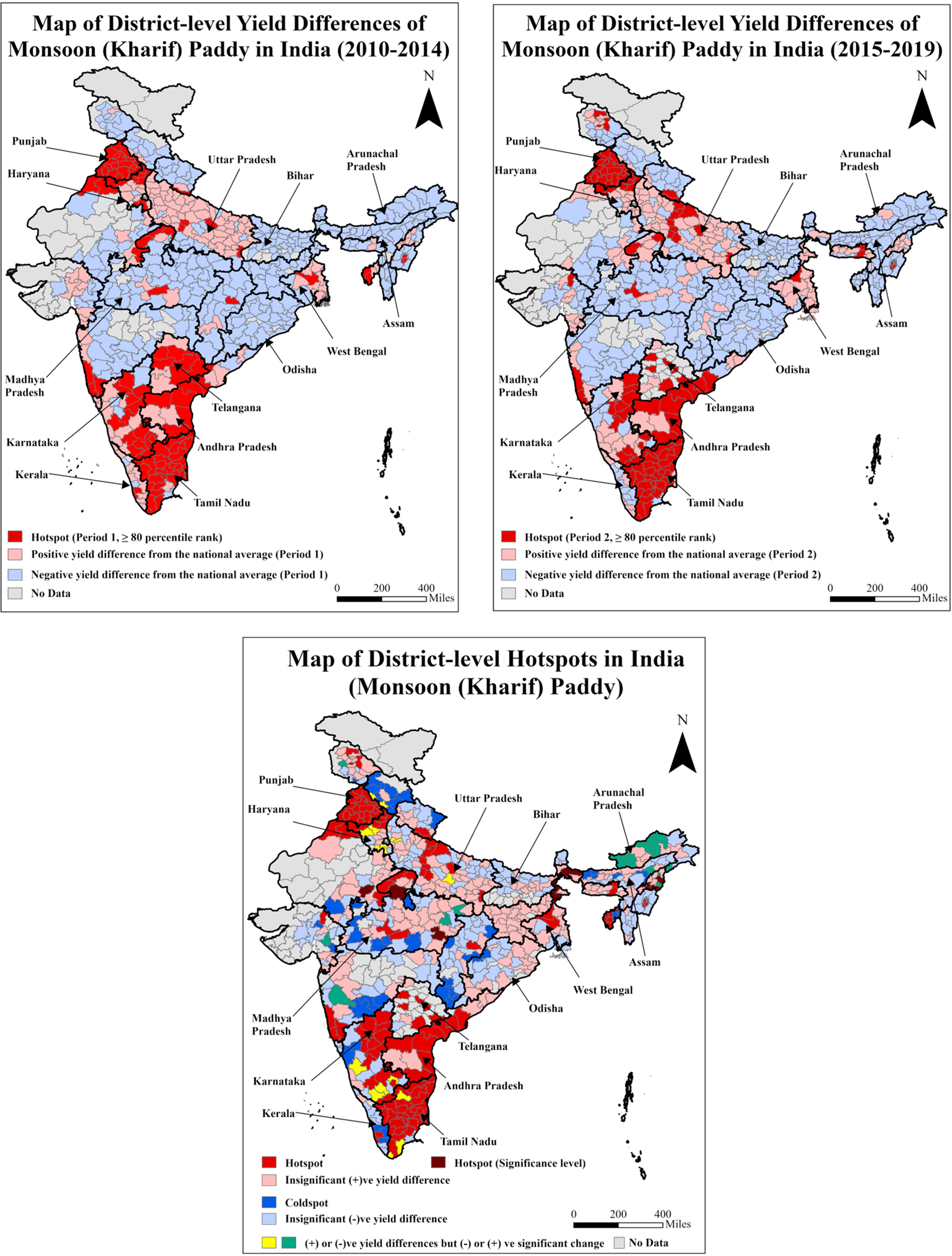
Figure 2 (I and II) shows the average differences in paddy yields following equation (1) for the monsoon season for periods 1 and 2, along with the periodic hotspots based on 80th percentile rank. In Figure 2 (III), we aggregate the hot/coldspot clusters for the monsoon paddy from both periods, as well as the significant yield positive/negative differences from period 1 to period 2. Besides hot/coldspots and insignificant positive/negative yield differences, we have cases in which positive/negative yield differences occur in both periods but with significant negative/positive changes. All these district categories are color-coded appropriately. The sequence of presenting yield differences by period and aggregate hotspot maps remains identical across the remaining seasons and crops. The monsoon paddy yield hotspot district clusters are located in the States of Punjab, Haryana, and Uttar Pradesh in the north, as well as in Telangana, Andhra Pradesh, Tamil Nadu, and Karnataka in the south, and in West Bengal in the east. In comparison, low-performing districts are clustered in the central, western, eastern, and northeastern States. While comparing the yield-difference maps for these two periods, the eastern Madhya Pradesh, Jharkhand, and eastern Odisha districts have observed an improvement in monsoon paddy yields. Although Bihar and Chhattisgarh, in the eastern and central regions, are in low-performing yield clusters. The total number of monsoon paddy yield hotspot and coldspot districts is 141 and 44, respectively. The average yield difference between these hotspot and coldspot districts is 2 t ha−1 (Table 3).
Maps of district-level yield differences for the two periods and hotspots for monsoon (Kharif) paddy of India.
Note: The third map presents the distribution of hotspot districts based on 80th percentile ranks in periods 1 and 2 and significant (+)ve yield difference between these periods. The coldspot districts are classified based on significant (−)ve yield differences between these periods. The average district-level yield of monsoon paddy nationwide is 2.16 t ha−1. The average yields of monsoon paddy for hotspot and coldspot districts are 3.32 and 1.34 t ha−1, respectively (Table 3).
Average seasonal crop yields and percentage KCC queries, average percentage gross irrigated area for the crops, fertilizer consumption per gross cropped area for the hotspot and coldspot districts based on yield performances
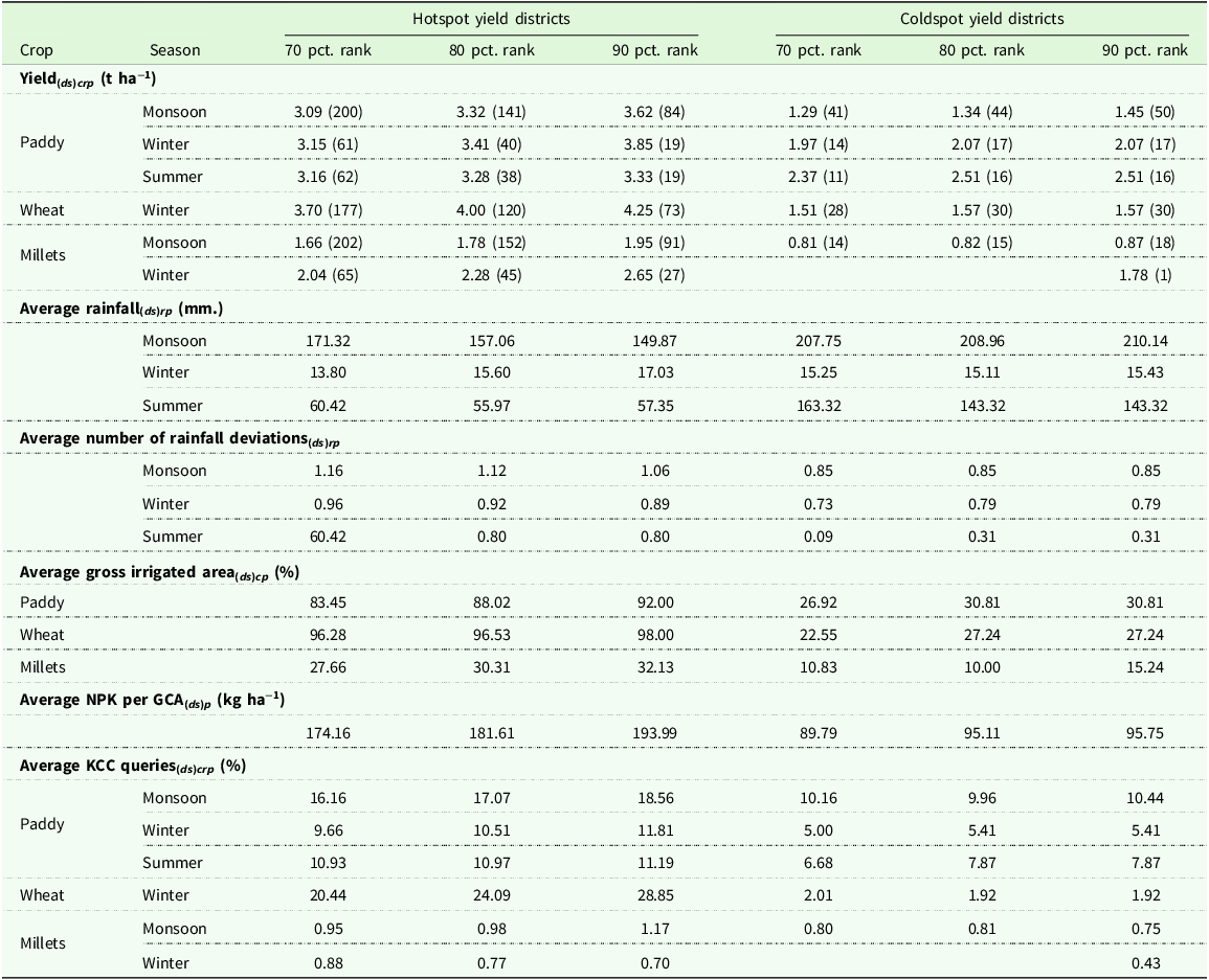
Note: Hotspot districts are classified whose yields are at and above the 80th (70th and 90th) percentile rank in any of the periods, or have significant positive yield differences from period 1 to period 2. Coldspot districts are those that have demonstrated significant negative yield differences from period 1 to period 2. The values in the parentheses are the number of observations for crop yield hot/coldspots districts. The percentages KCC queries are at the district level in respective States, based on seasons, years, and crops. d: District, s:State, c: Crop types (Paddy, Wheat, Millets), r: Season, p: Periods, KCC: Farmers (Kisan) call center.
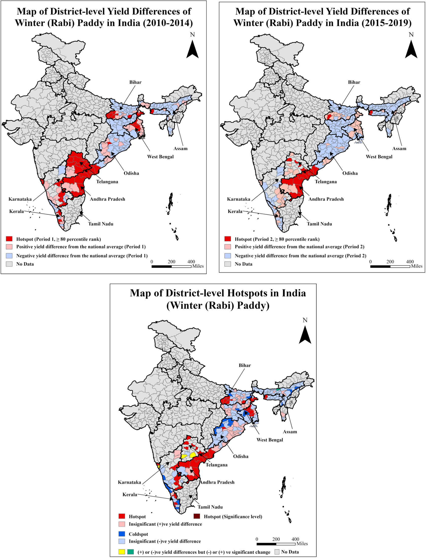
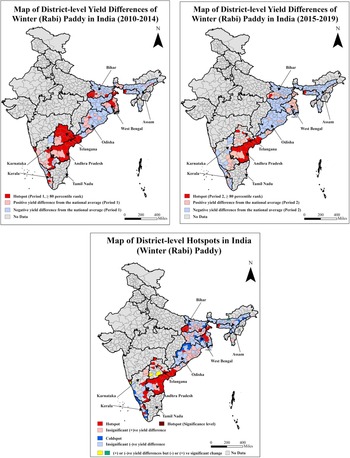
The winter season follows the monsoon cropping season. Figure 3 (I, II, and III) depicts the pattern of yield differences in two periods and the hotspot mapping for winter paddy. Winter paddy is cultivated in the southern, eastern, and northeast regions. High-yielding districts and hotspots are clustered in the States of Andhra Pradesh and Telangana in the southFootnote 8 and West Bengal in the east. The low-yielding districts are mainly concentrated in Bihar and Jharkhand in the east and Assam in the northeast. The average yield differences between the hotspot and coldspot districts (number of districts are 40 and 17, respectively) are narrower than monsoon paddy (1.34 t ha−1, Table 3).
Maps of district-level yield differences for the two periods and hotspots for winter (Rabi) paddy of India.
Note: The third map presents the distribution of hotspot districts based on 80th percentile ranks in periods 1 and 2 and significant (+)ve yield difference between these periods. The coldspot districts are classified based on significant (−)ve yield differences between these periods. The average district-level yield of winter paddy nationwide is 2.31 t ha−1. The average yields of winter paddy for hotspot and coldspot districts are 3.41 and 2.07 t ha−1, respectively (Table 3).
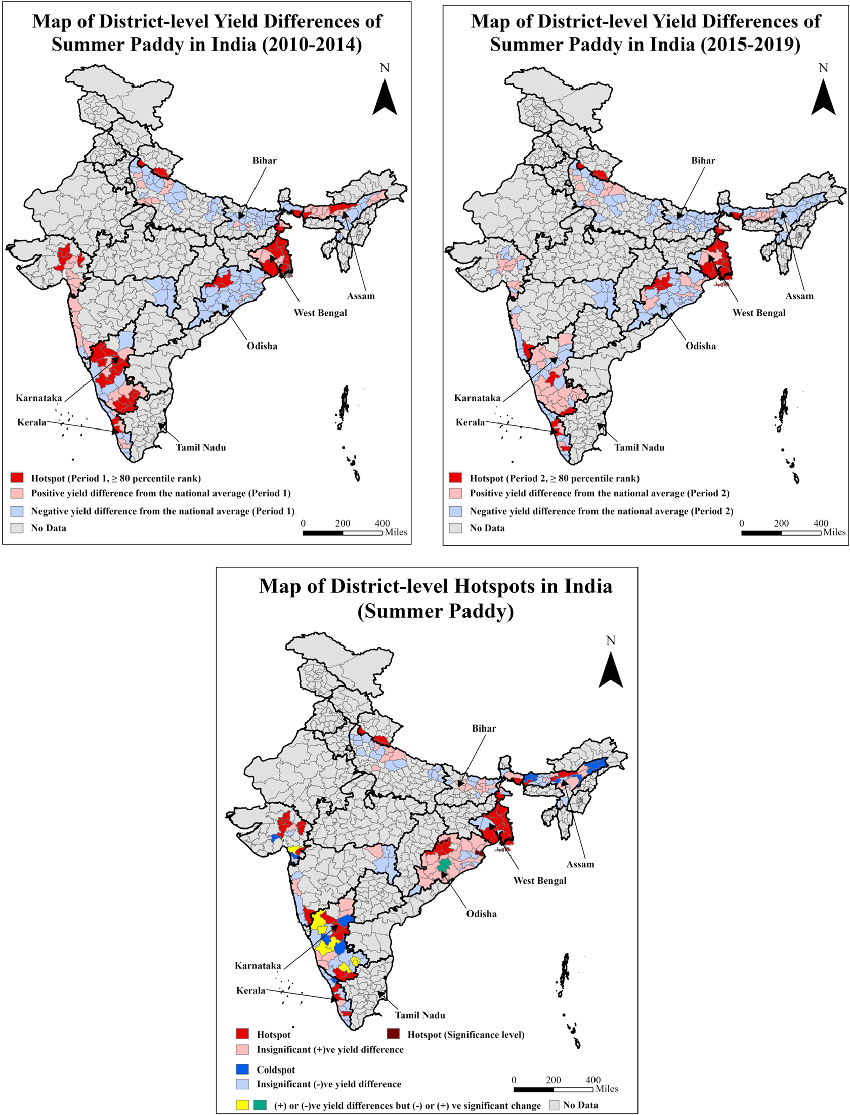
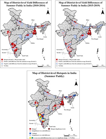
Summer paddy is cultivated mainly in West Bengal, Bihar, and Odisha in the east, Assam and Tripura in the northeast, and Karnataka and Kerala in the south.Footnote 9 Hotspot and high-yielding clusters are in the States of West Bengal and Karnataka, while the low-yielding clusters are concentrated in parts of Assam, Bihar, and Odisha (Figure 4: I, II, and III). But the districts of Bihar have improved on the paddy yields from period 1 to period 2. The eastern and northeastern regions focus on paddy cultivation year-round, but most States have low-performing clusters. The average yield difference in summer paddy between the hotspot and coldspot districts (the number of districts is 38 and 16, respectively) is 0.77 t ha−1, Table 3.
Maps of district-level yield differences for the two periods and hotspots for summer paddy of India.
Note: The third map presents the distribution of hotspot districts based on 80th percentile ranks in periods 1 and 2 and significant (+)ve yield difference between these periods. The coldspot districts are classified based on significant (−)ve yield differences between these periods. The average district-level yield of summer paddy nationwide is 2.62 t ha−1. The average yields of summer paddy for hotspot and coldspot districts are 3.28 and 2.51 t ha−1, respectively (Table 3).
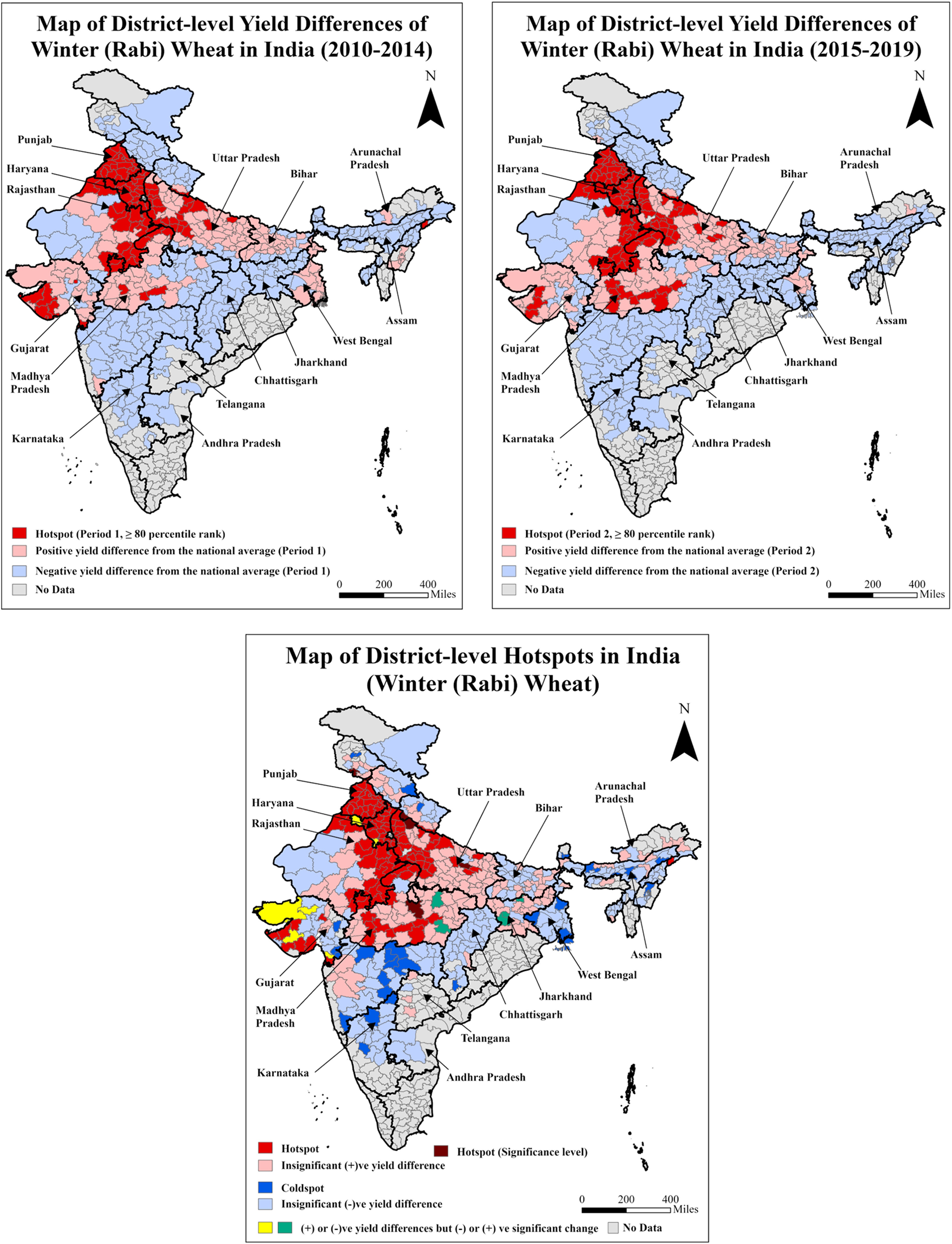
Wheat is a winter season crop grown in all regions except Tamil Nadu and Kerala in the South and Odisha in the east. Significant positive yield differences are observed in the State of Madhya Pradesh in the central region in period 2 relative to period 1, which are reflected in the hotspot map (Figure 5). The hotspot district clusters are in Punjab, Haryana, and Uttar Pradesh in the north, in Madhya Pradesh and central and eastern Rajasthan, and in western Gujarat. Wheat, a winter crop, depends on irrigation. Notably, the districts in the western and northern parts of Madhya Pradesh have shown a significant improvement in wheat yield. Improvements in irrigation systems and the implementation of State-level agricultural policies have boosted wheat yield growth in Madhya Pradesh (Gulati et al. Reference Gulati, Rajkhowa, Roy, Sharma, Gulati, Roy and Saini2021). The agricultural development success in Madhya Pradesh could serve as an effective model for States in eastern and northeastern India. On the other hand, low-performing and coldspot districts are concentrated in Maharashtra in the west, in West Bengal in the east, and in the southern and north-eastern States. The average yield difference in wheat (winter) among the hotspot and coldspot districts is highest among all the crops and seasons (2.4 t ha−1, with 120 and 30 hotspot and coldspot districts, respectively, Table 3).
Maps of district-level yield differences for the two periods and hotspots for winter (Rabi) wheat of India.
Note: The third map presents the distribution of hotspot districts based on 80th percentile ranks in periods 1 and 2 and significant (+)ve yield difference between these periods. The coldspot districts are classified based on significant (−)ve yield differences between these periods. The average district-level yield of winter wheat nationwide is 2.54 t ha−1. The average yields of winter wheat for hotspot and coldspot districts are 4.00 and 1.57 t ha−1, respectively (Table 3).
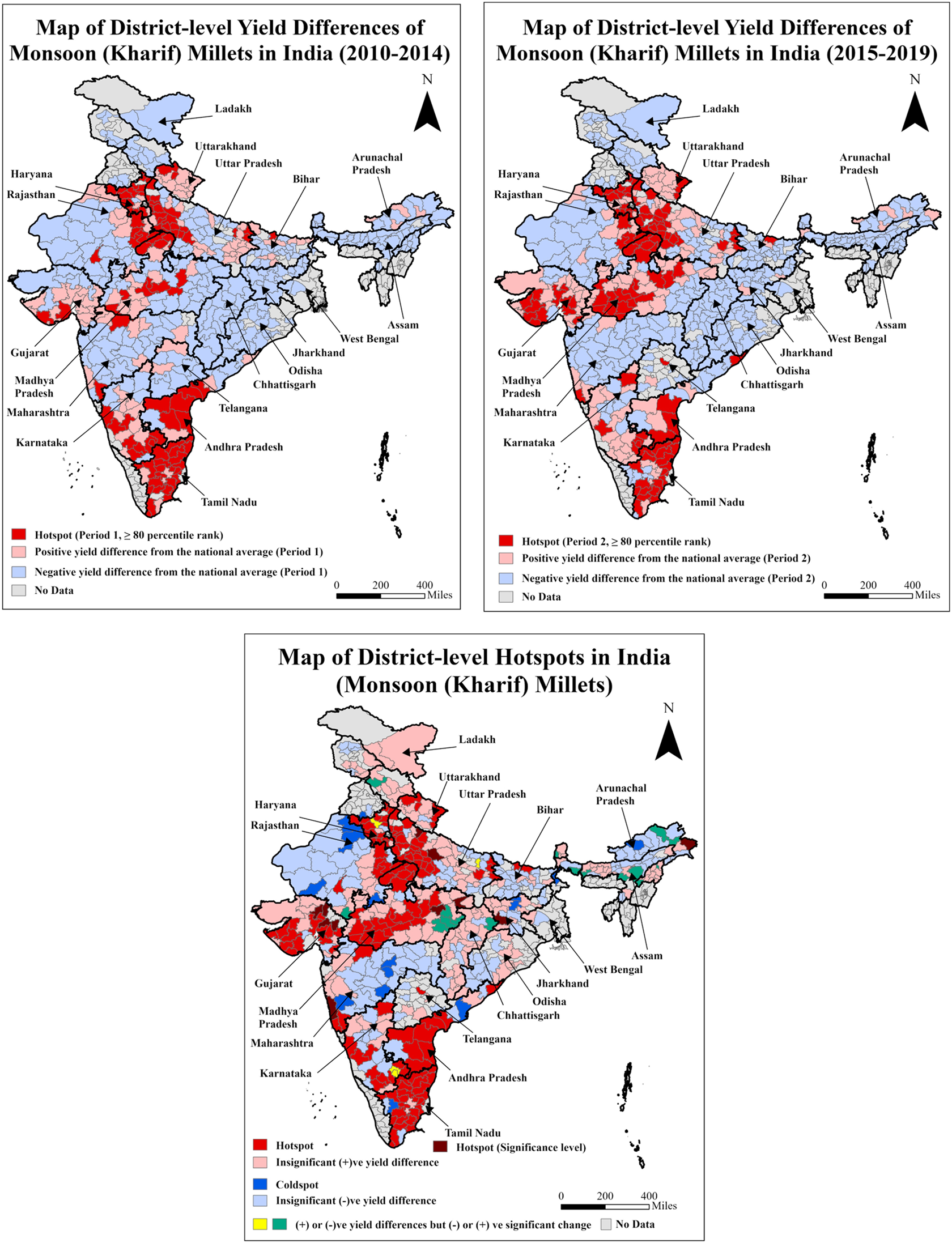
The third group of food grains, millets (comprised of Sorghum, Pearl millet, Finger millet, and Little millet), is widely cultivated throughout India during the monsoon season. The maps of the two-period yield differences and hotspot plots are shown in Figure 6 (I, II, and III). Positive yield differences and hotspots are clustered in the north-central region comprising neighboring districts from the States of Haryana, Uttar Pradesh, Rajasthan, and Madhya Pradesh, the southern region encompassing the States of Andhra Pradesh, Karnataka, and Tamil Nadu, and districts of eastern Gujarat in the west. The low-performing districts are clustered in the south-central, western, and eastern regions. Similar to wheat, Madhya Pradesh stands out in millet yields. The eastern region remains a low-productive cluster for coarse cereal production. The millets’ yields are lowest among all the crop types and seasons in both the 152 hotspot and 15 coldspot districts, with average yield differences of around 1 t ha−1, Table 3.
Maps of district-level yield differences for the two periods and hotspots for monsoon (Kharif) millets of India.
Note: The third map presents the distribution of hotspot districts based on 80th percentile ranks in periods 1 and 2 and significant (+)ve yield difference between these periods. The coldspot districts are classified based on significant (−)ve yield differences between these periods. The average district-level yield of monsoon millets nationwide is 1.15 t ha−1. The average yields of monsoon millets for hotspot and coldspot districts are 1.78 and 0.82 t ha−1, respectively (Table 3).
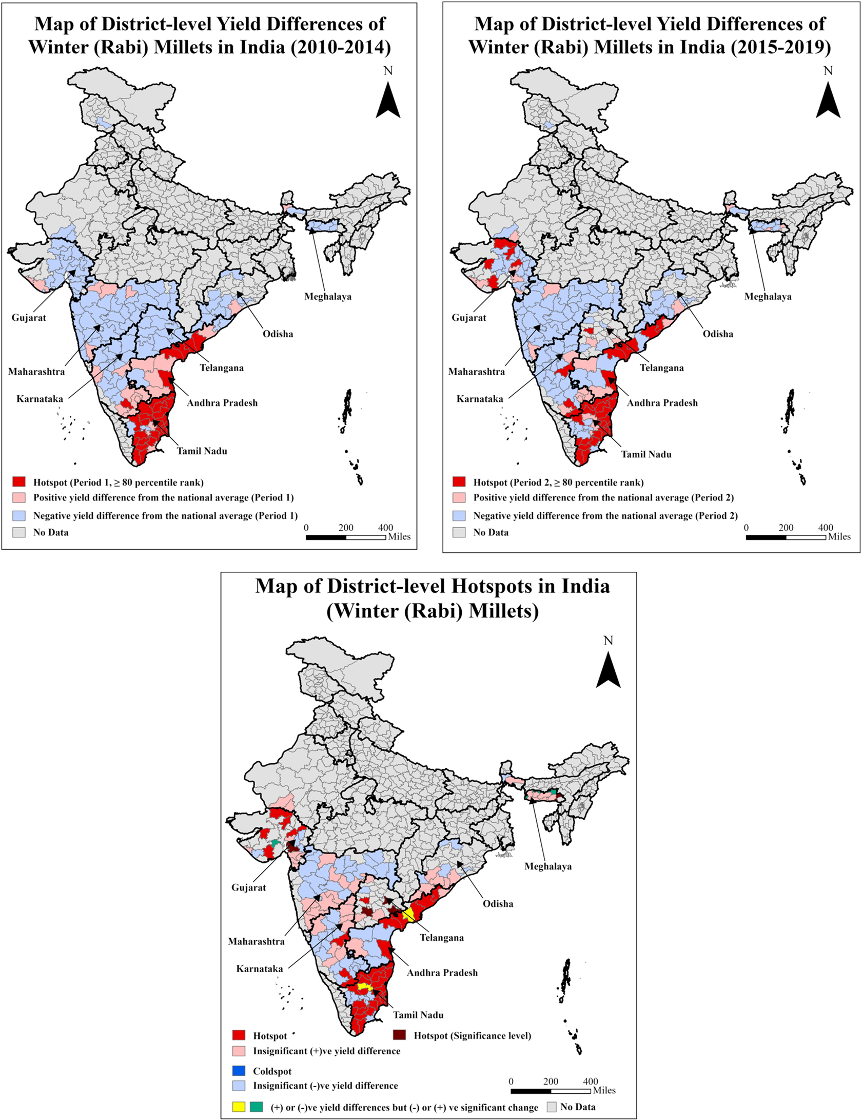
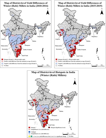
Winter millets are mainly cultivated in the western and southern regions (Figure 7). The high-yielding districts are concentrated in the States of Andhra Pradesh and Tamil Nadu, whereas the low-yielding districts are concentrated in Maharashtra in the west and Karnataka in the south. The results reflect a consistently similar picture of having southern dominance in crop yields.
Maps of district-level yield differences for the two periods and hotspots for winter (Rabi) millets of India.
Note: The third map presents the distribution of hotspot districts based on 80th percentile ranks in periods 1 and 2 and significant (+)ve yield difference between these periods. The coldspot districts are classified based on significant (−)ve yield differences between these periods. The average district-level yield of winter millets nationwide is 1.36 t ha−1. The average yield of winter millets for hotspot districts is 2.28 t ha−1 (Table 3).
The distribution of hotspot and cold spot districts based on narrower hotspot identification criteria (90th percentile rank and above for seasonal crop yields) are presented in the Appendix, Figures A.1, A.2 and A.3 for the crops paddy, wheat, and millets. The crop yields, weather, and input consumption metrics for these new hotspots and coldspots are summarized in Table 3. In this table, in addition to the 90th percentile, we report the 70th percentile to more clearly motivate the choice of the 80th percentile as the baseline for our main analysis. A more extensive justification of this classification metric is provided in Section 5, which presents the robustness checks.
Analysis of district-level weather deviations
Weather deviations play a vital role in seasonal paddy yields, along with agricultural inputs, in India. It has been widely reported that reductions in seasonal paddy yields due to drought and floods, along with deviations in temperatures (Auffhammer et al. Reference Auffhammer, Ramanathan and Vincent2012). We have plotted the average z-Scores of the weather deviations at the district level for maximum temperature, minimum temperature, and rainfall in the Appendix Figure B.1 (following equation 3). The northwestern, central, and southern States experienced the most weather deviations, along with the States of Bihar and Jharkhand in the east. On the other hand, the States in the north, West Bengal in the east, and the northeast experienced the least weather deviations. The findings are consistent with those of Saha et al. (Reference Saha, Chakraborty, Hazarika, Shakuntala, Das, Chhabra, Sadhu, Chakraborty, Mukherjee, Singson and Mishra2022). The weather deviations in the north-west and southern peninsula are due to El Niño and La Niña events. These events have negatively influenced the yields of major crops, including paddy (Bhatla et al. Reference Bhatla, Varma, Verma and Ghosh2020). Based on suggestive evidence, rainfall significantly affects crop yields. Thus, we further investigate observed rainfall and rainfall deviation hotspots using similar methodological techniques to those used for crop yield hotspots.
The seasonal rainfall deviation hotspot maps (i.e., monsoon, winter, and summer) based on historical rainfall data are shown in Figure B.2 in the Appendix. The hotspot clusters are scattered but mainly concentrated in the north across the seasons. The monsoon season’s rainfall deviation over the periods is mostly uniform across the country, with hotspot clusters in the northern and central States. On the other hand, in the winter, rainfall deviation hotspot clusters are in Gujarat (west), Punjab (north), Jharkhand (east), Tamil Nadu (south), and Assam (northeast). In summer, rainfall deviations are uniform across the country, except for clusters of districts in the adjoining States of Uttar Pradesh, Madhya Pradesh, Bihar, and northern Chhattisgarh. While comparing districts based on crop yield performance, greater rainfall deviations are observed in crop yield hotspots than in coldspots, in the following order: summer, monsoon, and winter (Table 3).
The observed seasonal rainfall hotspot maps are shown in Figure B.3 in the Appendix. In all three seasons, rainfall hotspots are concentrated in the northeastern States, and high rainfall is also observed in the States of West Bengal and Jharkhand in the eastern region, and in Tamil Nadu in the south. During the monsoon season, high-rainfall districts are concentrated in the east and central regions, with hotspot clusters in Odisha and Chhattisgarh. While in the winter season, we observe additional hotspot clusters in Punjab, Himachal Pradesh, and Uttarakhand. The central and south-central regions are in a low rainfall zone in winter. In the summer season, we observe high-rainfall clusters in the north and western regions and low-rainfall district clusters in the adjoining States of Uttar Pradesh, Madhya Pradesh, Bihar, and northern Chhattisgarh. The observed rainfall hotspot maps mostly echo the rainfall deviation maps. An interesting fact, the crop yield coldspot districts received more rainfall than the corresponding hotspot districts in monsoon and summer (i.e., average rainfall differences of 52 mm and 87 mm, respectively, Table 3). Thus, comparing observed rainfall and rainfall deviations, it is evident that these variables are unlikely to be significant factors in crop yield deviations. Irrigation coverage may be relevant to crop yield variations in India.
Analysis of inputs influencing crop yields
In this subsection, we discuss the findings of the hotspot analysis of the inputs: percentage gross irrigated area (aggregate and crop-wise), fertilizer consumption per gross cropped area, and farmers’ queries through mobile phones at KCC (crop and season-wise). The mapping of these input variables provides valuable insights into the formation of hot/coldspot clusters.
Analysis of district-level percentage of gross-irrigated area
We have mapped the average percentage of the gross irrigated area (aggregate) for each Indian district in the Appendix, Figure B.4. The districts of Punjab, Haryana, and Uttar Pradesh in the north and Bihar in the east are the most irrigated areas in India, followed by the districts of South India in the States of Telangana, Andhra Pradesh, and Tamil Nadu. On the other hand, the least irrigated districts are in the States of West Bengal (east), Maharashtra (west), and the North-eastern region. Next, we present crop-wise hotspot maps for the percentage gross irrigated area comparing two periods in the Appendix, Figure B.5. Paddy-irrigated hotspots are located in Uttar Pradesh (north), Bihar (east), and Tamil Nadu (south), whereas the coldspots are concentrated in the central and western regions. Hotspots for the wheat crop are concentrated in Gujarat (west) and Bihar (east), and coldspots are concentrated in Maharashtra (west). In the case of millets, coldspots are more prominent from the west to the central region (comprising States of Maharashtra, Rajasthan, Madhya Pradesh, and Chhattisgarh), and the hotspot districts are in Gujarat (west), Haryana (north), and Tamil Nadu (south). The paddy, wheat, and millets yield hotspot districts received 57%, 69%, and 20% more irrigation than the corresponding coldspot districts (Table 3). It confirms our claim in the previous section that irrigation significantly affects crop yield deviations.
Analysis of district-level fertilizer consumption per gross cropped area
Besides irrigation, fertilizer is an essential input for the crop yield differences. The Figure B.6 in the Appendix presents the district-level hotspots for the fertilizer consumption per gross cropped area. These hotspot clusters are in the northern districts of Punjab, Haryana, and Uttar Pradesh, expanding towards Bihar in the east. Another cluster of hotspots is in the southern districts of Telangana, Andhra Pradesh, and Tamil Nadu. The fertilizer coldspot and low fertilizer consumption clusters are spread across central and western India. On average, hotspot yield districts consume 86.5 kg ha−1 more fertilizer than that of crop yield districts (Table 3), similar to the irrigation coverage trend.
Analysis of district-level percentage crop-specific KCC queries
Information is a vital input, along with irrigation and fertilizer, for crop production. The use of mobile phones by farmers to access agricultural information from KCC enhances crop yield in India (Gupta et al. Reference Gupta, Ponticelli and Tesei2024; Pramanik Reference Pramanik2026). The incidence of KCC queries also serves as a proxy for technology transfer and for scientific and knowledge-based cropping systems. We have classified the KCC queries by crop (i.e., paddy, wheat, and millets) and season for our analysis. The percentage of district-level queries for the respective crops and seasons in the corresponding States is estimated for each year of the study period (2010–2019). We then apply similar hotspot estimation methods to classify the KCC queries as hotspot/high-performing or coldspot/low-performing districts by season and crop. In the case of paddy, hotspot clusters are spread across paddy-growing areas in Odisha (east), Telangana, and Andhra Pradesh in the south, and Punjab in the north, across seasons (see Appendix Figure B.7). North-eastern districts also contribute to the hotspot clusters. Interestingly, Bihar’s districts are placing fewer queries at the KCCs than irrigation usage and fertilizer consumption do across seasons. Based on cropping seasons (monsoon, winter, and summer) of paddy, the average percentage KCC queries differences among crop-yield hotspot (17%, 11%, and 11%)Footnote 10 and coldspot districts are 7%, 5%, and 3%, respectively (Table 3).
When comparing the percentage of district-level queries for wheat during the winter season, the hotspot clusters are located in the central region of Madhya Pradesh (see Appendix Figure B.9). The percentage of queries for wheat is decreasing in the wheat-growing areas in Punjab, Haryana, and Uttar Pradesh. The districts of Bihar still report fewer wheat-related queries during the winter season. The average percentage KCC query difference among hotspot (24%)Footnote 11 and coldspot yield districts for winter wheat is 22% (Table 3).
The millet-related queries are reported in the monsoon and winter seasons. The hotspot district clusters are in the southern (Tamil Nadu and Karnataka), western (Maharashtra and Gujarat), and northern (Punjab and Haryana) regions. In addition to the hotspot clusters, the millet-related queries are increasing from period 1 to period 2 across India. The average percentage KCC query difference among hotspot (0.98%),Footnote 12 and coldspot yield districts for millets is 0.17% (Table 3).
Relation between crop yield differences and influencing factors
In this section, we explore the relationship between weather and input factors that influence crop yield differences. Irrigation contributes to crop yields but is linked to deviations in rainfall coverage. Thus, we first regress the percentage of gross irrigated area on rainfall and deviations from historical averages; the regression results are presented in Table 4. Irrigation coverage is positively and significantly related to rainfall deviations in both scenarios when regressed individually and together with rainfall. The relationship between irrigation coverage is negative but not statistically significant. It supports the suggestive evidence that districts with greater rainfall deviations require more irrigation coverage, and the districts with less observed rainfall require more irrigation coverage.
Relation between rainfall and irrigation coverage in India
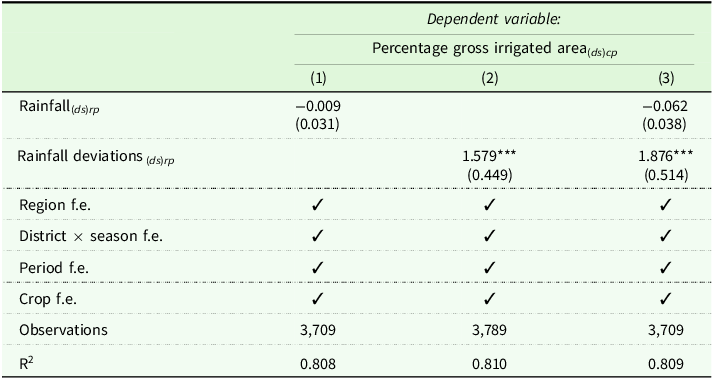
Note: All the regressions are based on data at the district-level for two periods (Period 1: 2010–2014 and Period 2: 2015–2019). Column (1) represents the regression results between the crop-specific average period-level percentages of gross irrigated area and average rainfall based on seasons and periods. Similarly, column (2) is the regression results between crop-specific irrigation coverage and rainfall deviations. Column (3) is the regression results when observed rainfall and rainfall deviations are regressed with crop-specific irrigation coverage. All regression equations include Region, district × season, Period, and Crop fixed effects. Standard errors are clustered at the district level and are reported in parentheses. The full regression table that demonstrates the estimates for the fixed effects (crop and period) is in the Appendix, Table C.1. d: District, s: State, c: Crop types (Paddy, Wheat, Millets), r: Season, p: Periods.
Significance level: *p < 0.1; **p < 0.05; ***p < 0.01.
Next, we explore the relationships between the weather (especially, rainfall and rainfall deviations) and input factors (percentage crop-specific gross irrigated area, fertilizer consumption, and percentage crop-specific KCC queries) with respect to the crop yield deviations. The regression results are presented in Table 5. The first five columns explore the relationships with rainfall and input factors without other weather controls (i.e., minimum and maximum temperatures and their respective deviations). The results are consistent with (columns (6) and (7)) and without (columns (1) to (5)) the controls. In column 7, we excluded the rainfall deviation because it was strongly correlated with irrigation coverage. All input factors are positively related to yield deviations, along with rainfall, but negatively related to rainfall deviations. These relationships are statistically significant. The results suggest that increases in input factors and rainfall lead to positive deviations in yield and thus to hotspot clusters. In contrast, deviations in rainfall negatively impact the formation of hotspot clusters. An additional 1% irrigation coverage for a specific crop type, a 1% rise in crop-specific queries to the KCC, and an extra kg ha−1 of fertilizer at the district level are associated with an increase in yield differences by 7, 6, and 0.5 kg ha−1, respectively. Although the extensive set of fixed effects and control variables substantially reduces the risk of confounding, several forms of endogeneity are likely to remain. These include omitted variable bias – for instance, from unobserved variation in soil characteristics or farm management practices – reverse causality, whereby higher yields may themselves facilitate subsequent expansion of irrigation infrastructure, and selection bias arising if irrigated plots differ systematically from non-irrigated plots along unmeasured dimensions. Consequently, the estimated coefficients should be interpreted as conditional correlations rather than as strictly causal parameters.
Factors influencing crop yields in India
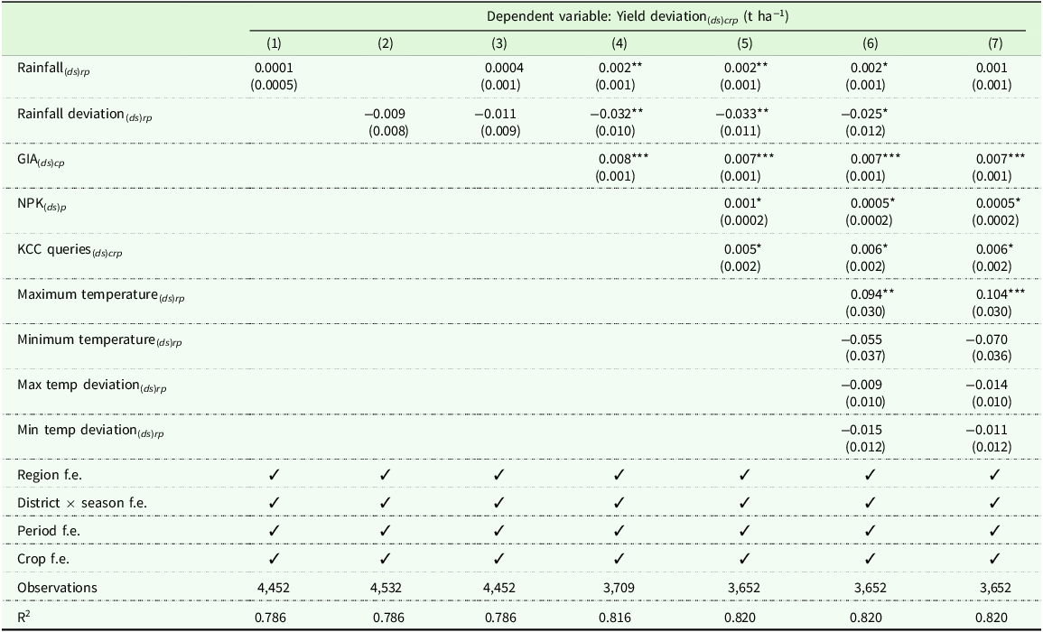
Note: All the regressions are based on data at the district-level for two periods (Period 1: 2010–2014 and Period 2: 2015–2019). Columns (1) to (4) display the relation between seasonal crop yield deviations and rainfall, rainfall deviations, and crop-specific percentage gross irrigated area. In column (5), we include other input factors (fertilizer consumption and the percentage of KCC queries). Column (6) includes other weather variables as controls (maximum temperature, minimum temperature, and their average historical deviations). In column (7), we only exclude rainfall deviation as irrigation and rainfall deviation are significantly correlated (Table 4). There is no significant change in estimates when comparing column (6) and column (7). All regression equations include district × season, Period, and Region fixed effects. Standard errors are clustered at the district level and are reported in parentheses. The full regression table that demonstrates the estimates for the fixed effects (crop and period) is in the Appendix, Table C.2. GIA: Gross Irrigated Area, NPK: Total Fertilizer consumption (GCA) per Gross Cropped Area (GCA), KCC: Farmers (Kisan) call center, d: District, s: State, c: Crop types (Paddy, Wheat, Millets), r: Season, p: Period. Significance level: *p < 0.1; **p < 0.05; ***p < 0.01.
It is also evident from the Table 3 that the yield across major crop-growing seasons is double in hotspot districts compared to coldspot districts. Similarly, significant differences in input consumption are observed between hotspot districts and coldspot districts. Coldspot districts are 60% less irrigated for paddy and wheat cultivation and around 20% less irrigated for millet cultivation. Coldspot districts consume 100 kg ha−1 less fertilizer per gross cropped area than hotspot districts. On the other hand, the percentage differences in information access between hotspot and coldspot districts for the paddy crop vary between 3% and 7%; for wheat, it is 22%; and for millets, it is 0.17%. This comparative analysis further justifies the findings in the regression analysis.
Discussion of results
The analyses reveal the clustering of districts based on seasonal crop yields, with identifiable regional crop yield hotspots and coldspots, as well as similar clusters based on weather and input factors influencing yield. The all-India analysis identifies specific States and regions for further district-level analysis to pinpoint the drivers of high- and low-yielding clusters. Although this study delineates regions that are significantly high- and low-performing, States, and districts, evaluating the detailed causal directions underlying clustering is beyond the scope of this paper. However, these findings establish the foundation for examining a critical research question: Why do some districts have higher yield potential than others, irrespective of weather conditions?
The analyses confirm districts of Punjab, Haryana, and Uttar Pradesh in the north, Tamil Nadu, Karnataka, Andhra Pradesh, and Telangana in the south, and West Bengal in the east are consistent high-yielding hotspots for paddy. Although Odisha and Madhya Pradesh are in low-yielding clusters, the districts of these States have observed an improvement in seasonal paddy yields over the period. In addition to irrigation and rainfall, farmers’ queries at KCC for paddy have increased from period 1 to period 2 in Madhya Pradesh and Odisha, especially during the monsoon season. For wheat, hotspot clusters are concentrated in Punjab, Haryana, and Uttar Pradesh in the north, along with the adjoining districts of Rajasthan and Gujarat in the west and in Madhya Pradesh in the central region. Therefore, the north and central regions are wheat hotspot zones. Districts in northern and western Madhya Pradesh have observed significant positive changes in wheat yields. Madhya Pradesh wheat yield growth reflects a significant increase in wheat-related queries at KCC from period 1 to period 2, as well as an improvement in wheat irrigation coverage. Millets yield in the monsoon and winter seasons. The north-central districts adjoining Haryana, Rajasthan, Uttar Pradesh, and Madhya Pradesh, Gujarat in the west, and Tamil Nadu and Andhra Pradesh in the south, are the hotspot centers of millet yields. In addition to irrigation clusters for millets in the north and south, KCC queries for millets coincide with millets’ yield hotspots. This further emphasizes that information plays an important role in crop yields besides weather, irrigation coverage, and fertilizer consumption.
The districts in the States of Maharashtra in the west, Chhattisgarh in the central, Bihar, Odisha, and Jharkhand in the east, and the northeast States are consistently in low-performing or coldspot clusters irrespective of the seasons and food grains in this study. Additionally, Table 2 summarizes regional performances across different seasons and crops, aligning with the classification of regions as progressive or lagging, as described in Pingali et al. (Reference Pingali, Aiyar, Abraham and Rahman2019). Crop yield performance in the west, east, and central regions can contribute to overall national yield performance across crops and seasons.
On the other hand, the higher percentages of the average gross irrigated lands are predominantly located in the districts of Punjab, Haryana, Uttar Pradesh, Bihar, Telangana, Andhra Pradesh, and Tamil Nadu, as depicted in the Appendix Figures B.4 and B.5. In evaluating crop yield data against the backdrop of weather anomalies and rainfall patterns, it becomes apparent that the southern states have achieved outstanding agricultural outcomes. This success can largely be attributed to their extensive use of irrigation systems, increased fertilizer application, and enhanced access to agronomic information provided by the KCC via mobile phones. Conversely, the districts of West Bengal exhibit a relatively lower percentage of gross irrigated areas due to their dependency on rainfed agricultural practices. Nonetheless, there is potential for yield improvements with increased fertilizer use and improved information outreach through KCC or alternative information dissemination platforms. Furthermore, while Bihar’s districts demonstrate extensive irrigation coverage and substantial fertilizer usage, they report a limited number of inquiries at the KCC, which correlates with modest yield outcomes. It is evident that districts endowed with favorable climatic conditions, supplemented by robust irrigation infrastructure, high fertilizer inputs, and efficient access to agricultural information via KCC, represent the concentration of highly productive agricultural clusters. Therefore, the synergistic operation of these components holds substantial promise for enhancing India’s food grain production capabilities.
To comprehensively assess the associations between these input parameters and variations in agricultural yield, as shown in Table 5, specific district-level factors appear particularly important. Specifically, a one-unit higher percentage of irrigation coverage dedicated to a particular crop type at the district level, a one-unit higher district-level percentage of crop-specific queries to the KCC, and an additional kg ha−1 of fertilizer application are each associated with 7, 6, and 0.5 kg ha−1 higher yield differences, respectively, conditional on the included covariates and fixed effects. This pattern highlights the potential importance of targeted agricultural practices and resource allocation for yield outcomes, though endogeneity from omitted variables, reverse causality, or selection may persist, limiting causal interpretation. It is to be noted that crop yield coldspots or low-performing districts would need to double their respective crop yields to become crop yield hotspots (Table 3).
The findings distinguish between short-term, information-based interventions – such as expanding crop-specific KCC queries, which are associated with 6 kg ha−1 higher yields – and structural investments like irrigation infrastructure (7 kg ha−1) and fertilizer supply chains (0.5 kg ha−1 per kg ha−1 applied). For low-performing (coldspot) districts in drought-prone regions, policymakers should prioritize immediate digital extension scaling via mobile platforms to boost farmer knowledge, alongside medium-term irrigation expansion targeting paddy and wheat belts. In millets-growing arid areas, fertilizer subsidies paired with region-specific soil testing could yield faster gains, with coldspots needing double yield increases to match hotspots - feasible through phased public–private partnerships.
To illustrate, consider the district of Darbhanga in northern Bihar, which persistently exhibits under low-performing crop yield clusters.Footnote 13 Should the yields of paddy and wheat be elevated to match those characteristic of hotspot districts, the revenue could potentially escalate from Rs. 18,600 to Rs. 41,416 ha−1 for paddy, and from Rs. 35,376 to Rs. 62,645 ha−1 for wheat. Consequently, this improvement in yields is projected to enhance the revenue per household engaged in paddy cultivation from Rs. 2,757 to Rs. 6,850 and for those cultivating wheat from Rs. 5,038 to Rs. 9,003.
Robustness checks
To investigate hotspot identification sensitivity, we altered the hotspot identification criteria, moving from districts above the 80th percentile to those above the 90th and 70th percentiles for seasonal crop yields. The variation in metrics – specifically crop yields, weather patterns, and input utilization – between these three hotspot categories and their corresponding coldspots is shown in Table 3. Observed yield variations across different crops and seasons do not exceed 0.44 t ha−1. The yield differences between hotspot and coldspot districts, evaluated at the 80th to 90th and 70th to 80th percentile criteria levels, varies depending on criteria and main cropping seasons: Monsoon Paddy (2.18 and 1.80 t ha−1), Winter Wheat (2.68 and 2.19 t ha−1), and Monsoon Millets (1.08 and 0.85 t ha−1). The difference in the number of hotspot districts between similar comparison levels is approximately 50. Furthermore, the average input levels increase with the percentile criteria, and the same holds for rainfall and rainfall deviations, reflecting monotonic relationships. The selection of the percentile ranking criteria depends on the objective of precision. To further illustrate our selection of the 80th percentile ranking criteria for our analysis, we now examine the characteristics of districts with 80th- and 90th- percentile (higher) ranking criteria using crop yield hotspot maps.
When examining the yield maps across various crops and seasons, some differences emerge between the two types of hotspot yield maps referenced (Figures 3–7 and in the Appendix, Figures A.1 to A.3). While comparing paddy yield maps, hotspot distributions generally remain uniform across seasons; however, notable exceptions are observed, with fewer hotspot districts in West Bengal when the 90th-percentile criterion is employed. Compared with wheat yield maps, fewer hotspots are detected in the north-central zone, particularly in the States of Madhya Pradesh and Uttar Pradesh. For millets, a similar reduction in hotspots is observed in the central and southern regions, namely Madhya Pradesh and Andhra Pradesh. Hotspot ranking criteria are sensitive to districts transitioning into higher crop yield categories. To capture the performance of these transitioning districts, we use the 80th-percentile ranking criterion rather than the 90th-percentile criterion. The 70th-percentile criterion will be more relaxed and include districts that are just above average in performance.
Conclusion
The formation of high- and low-performing district clusters gives rise to hot- and coldspot clusters, as revealed by the all-India analysis of seasonal food grain crops. This phenomenon is rooted in the geographical placement of districts within agro-climatic zones, as well as in the influence of varying weather patterns, disparities in input consumption and agricultural land utilization, infrastructure availability, and information networks on agriculture. In this paper, we have compared crop yield differences with weather variability, gross irrigated area, fertilizer consumption, and demand for information at farmers’ call centers (i.e., KCC) as reflected in farmers’ queries. In particular, northern States exhibit fewer weather deviations, more irrigated districts, and clusters of crop yield hotspots. Meanwhile, clusters of weather deviations predominantly populate the western, central, and southern regions. But the southern districts stand out as hubs for paddy and millet cultivation because of relatively high irrigation facility usage, fertilizer consumption, and greater access to information from KCC. At the same time, the northeastern States with the least weather deviations and high rainfall incidence remain among the low-performing zones in India. Irrigation facilities, fertilizer consumption, and information access are crucial factors for crop yield growth. However, efficient management practices supported by advanced information networks can mitigate the influence of weather anomalies and advance regional development.
South Indian and Madhya Pradesh districts can serve as examples for the districts of Maharashtra, Chhattisgarh, Jharkhand, Bihar, and Odisha. Specifically, Bihar’s high input usage, such as irrigation and fertilizer, along with fewer KCC queries, continues to be classified as low-performing for crop yields. The combined use of inputs and access to agricultural information from scientific sources (such as KCC) is beneficial for aspiring hotspot districts in India. For coldspot or low-performing districts to transform into hotspots, they must significantly expand input levels and multiply KCC usage for scientific and knowledge-based cropping practices. Following hotspot transformation, representative households in a low-performing district in Bihar, growing paddy and wheat, can increase their revenue by 148% and 79% respectively. Strategic integration of infrastructure, inputs, and information is key to overcoming climatic challenges and promoting regional agricultural advancement.
Supplementary material
The supplementary material for this article can be found at https://doi.org/10.1017/age.2026.10029.
Data availability statement
The data used for the analysis are drawn from multiple sources, especially the Indian government and the International Crops Research Institute for the Semi-Arid Tropics (ICRISAT) websites on crop yields, agricultural input use, and access to digital agricultural information. Weather-related data is from the TerraClimate database. These datasets are merged at the district and season level for our analysis. The merged data and the R code used for the analysis will be made available upon request.
Acknowledgements
I am thankful to Arnab Basu, Prabhu Pingali, John Carruthers, Patrick Hatzenbuehler, and seminar participants at Cornell University for their valuable comments and feedback. I am especially grateful to the editor and the anonymous reviewer, whose comments and thoughtful suggestions significantly sharpened and strengthened this paper. I also gratefully acknowledge the institutional support from the University of Idaho-Idaho Experimental Station, Tata-Cornell Institute for Agriculture and Nutrition, and Cornell University.
Funding statement
This work was supported by the Graduate School and Department of City and Regional Planning, Cornell University, and the Tata Cornell Institute of Agriculture and Nutrition.
Competing interests
The author declare none.


 Open access