


1 Introduction
The notion of fractional Brownian motion (FBM) was introduced by Mandelbrot and Van Ness in 1968 [Reference Mandelbrot and Van Ness31]. The Hurst parameter H can be used to define the Hölder regularity of the FBM [Reference Ayache and Véhel7]. The multifractional Brownian motion (MBM) was first considered by Péltier and Lévy Véhel in 1995, extending the FBM [Reference Péltier and Véhel38]. The concept of multifractionality allows local fractional properties to depend on space-time locations. Multifractional processes were used to study complex stochastic systems which exhibit nonlinear behaviour in space and time. Multifractional behaviour of data has been found in many applications, such as image processing, stock price movements and signal processing [Reference Ayache and Véhel7, Reference Sheng, Chen and Qiu41].
The generalized multifractional Brownian motion (GMBM) is a continuous Gaussian process that was introduced by generalizing the traditional FBM and MBM (see [Reference Ayache and Véhel7]). In comparison to MBM, the Hölder regularity of GMBM can vary substantially. For example, GMBM can allow discontinuous Hölder exponents. This has been an advantage in certain applications, such as medical image modelling, telecommunications, turbulence and finance, where the pointwise Hölder exponent can change rapidly. A Fourier spectrum’s low frequencies control the long-range dependence of a stochastic process while the higher frequencies control the Hölder regularity. Therefore, GMBM can be used to model processes that exhibit erratic behaviour of the local Hölder exponent and long-range dependence [Reference Ayache and Véhel7].
The aim of this paper is to introduce new applied methodology based on the local Hölder exponent, and illustrate it by applying it to cosmic microwave background (CMB) radiation data. The following brief physics background is provided to enable a better understanding of the CMB data.
The universe originated about 14 billion years ago and was characterized by an extremely high temperature. The cosmological theory that is generally accepted is given, for example, in the book by Weinberg [Reference Weinberg45]. From $10^{-35}$
seconds (s) after the original singularity up to
$10^{-35}$
seconds (s) after the original singularity up to $10^{-32}$
s, there was rapid exponential inflation by a factor greater than
$10^{-32}$
s, there was rapid exponential inflation by a factor greater than $e^{60}$
, driven by an as yet unidentified inflation quantum field. Correlation lengths following from vacuum energy fluctuations rapidly expanded to separations that are now observed in the CMB to be well beyond the horizon of light signals. Inflation is an answer to the horizon puzzle as well as the flatness puzzle and the absence of magnetic monopoles. From
$e^{60}$
, driven by an as yet unidentified inflation quantum field. Correlation lengths following from vacuum energy fluctuations rapidly expanded to separations that are now observed in the CMB to be well beyond the horizon of light signals. Inflation is an answer to the horizon puzzle as well as the flatness puzzle and the absence of magnetic monopoles. From $10^{-5}$
s after the singularity, hadron particle–antiparticle pairs could form, followed by lepton pairs from 1 s. By 10 s, the universe had cooled enough so that pair annihilation led to photons being the dominant component of energy within the plasma for the next 380,000 years. During this time, within the plasma, the photon mean free path was relatively short, so the system was opaque. However, from 100,000 years onwards, He atoms and then neutral H atoms began to form. In the final stage of “recombination”, at temperature almost 4000 kelvin (K), after 378,000 years the photons propagated freely and can be observed in the CMB. Due to cosmological expansion, their wavelengths have now stretched to the microwave part of the electromagnetic spectrum, exhibiting a high-accuracy blackbody spectrum of a thermalized environment, matching with a temperature of 2.725 K. However, small anisotropic perturbations of that temperature are now of most interest. They indicate large-scale density variations within the plasma universe that are associated with preferred locations in the subsequent formation of galaxies. Further back, anisotropy relates to the formation of matter, separating rival quantum field theories.
$10^{-5}$
s after the singularity, hadron particle–antiparticle pairs could form, followed by lepton pairs from 1 s. By 10 s, the universe had cooled enough so that pair annihilation led to photons being the dominant component of energy within the plasma for the next 380,000 years. During this time, within the plasma, the photon mean free path was relatively short, so the system was opaque. However, from 100,000 years onwards, He atoms and then neutral H atoms began to form. In the final stage of “recombination”, at temperature almost 4000 kelvin (K), after 378,000 years the photons propagated freely and can be observed in the CMB. Due to cosmological expansion, their wavelengths have now stretched to the microwave part of the electromagnetic spectrum, exhibiting a high-accuracy blackbody spectrum of a thermalized environment, matching with a temperature of 2.725 K. However, small anisotropic perturbations of that temperature are now of most interest. They indicate large-scale density variations within the plasma universe that are associated with preferred locations in the subsequent formation of galaxies. Further back, anisotropy relates to the formation of matter, separating rival quantum field theories.
On a sphere, a scalar function such as temperature is most conveniently expanded in a basis of spherical harmonics in polar coordinates $Y_l^m(\theta ,\varphi )$
. The largest variation from isotropy is a dipole structure at
$Y_l^m(\theta ,\varphi )$
. The largest variation from isotropy is a dipole structure at $l=1$
. That dipole can be transformed away by choosing a reference frame that has a speed of 368 km/s relative to our own frame. There is significant structure in the spherical harmonic spectrum up to at least
$l=1$
. That dipole can be transformed away by choosing a reference frame that has a speed of 368 km/s relative to our own frame. There is significant structure in the spherical harmonic spectrum up to at least $l=1000$
. There is a consistent interpretation that we are now in a dark-energy-dominated era, consisting of 73% or more of the mass energy, around 23% dark matter, the small but important remainder being ordinary matter and radiation.
$l=1000$
. There is a consistent interpretation that we are now in a dark-energy-dominated era, consisting of 73% or more of the mass energy, around 23% dark matter, the small but important remainder being ordinary matter and radiation.
In the microwave region, the CMB spectrum closely follows that of a black body at equilibrium temperature 2.735 K, tracing back to a plasma temperature of around 4000 K at a time corresponding to redshift $z =1500$
at 50% atomic combination. Although the equilibrium spectrum is essential, there are important departures from equilibrium that give information on the state of the early universe. Relative anisotropic variations of spectral intensity from that of a black body are of the order of
$z =1500$
at 50% atomic combination. Although the equilibrium spectrum is essential, there are important departures from equilibrium that give information on the state of the early universe. Relative anisotropic variations of spectral intensity from that of a black body are of the order of $10^{-4}$
. Calculations by Khatri and Sunyaev [Reference Khatri and Sunyaev25] showed that outside of a relatively small range of redshifts, external energy inputs from sources such as massive particle decay would dissipate by Compton and double Compton scattering and other relaxation processes to affect the signal by several lower orders of magnitude. The primary sources of anisotropy were large-scale acoustic waves whose compressions in the plasma universe were associated with raised temperatures. Using the current angular widths of anisotropies in the CMB, the current standard model
$10^{-4}$
. Calculations by Khatri and Sunyaev [Reference Khatri and Sunyaev25] showed that outside of a relatively small range of redshifts, external energy inputs from sources such as massive particle decay would dissipate by Compton and double Compton scattering and other relaxation processes to affect the signal by several lower orders of magnitude. The primary sources of anisotropy were large-scale acoustic waves whose compressions in the plasma universe were associated with raised temperatures. Using the current angular widths of anisotropies in the CMB, the current standard model $\Lambda $
CDM (cold dark matter plus dark energy) affords an estimate of the Hubble constant at
$\Lambda $
CDM (cold dark matter plus dark energy) affords an estimate of the Hubble constant at $H_0=67.4\pm 1.4$
km/s/MPc [Reference Aghanim4]. This agrees well with data from the POLARBEAR Antarctica telescope that give
$H_0=67.4\pm 1.4$
km/s/MPc [Reference Aghanim4]. This agrees well with data from the POLARBEAR Antarctica telescope that give $H_0=67.2\pm 0.57$
km/s/MPc [Reference Adachi2]. However, estimates from more recent emissions from closer galaxies, using both cepheid variables and type Ia supernovae as distance markers, give
$H_0=67.2\pm 0.57$
km/s/MPc [Reference Adachi2]. However, estimates from more recent emissions from closer galaxies, using both cepheid variables and type Ia supernovae as distance markers, give $H_0=74.03\pm 1.42$
km/s/MPc [Reference Riess, Casertano, Yuan, Macri and Scolnic40]. This unexplained discrepancy will eventually be resolved by newly found errors in the methodology of one or both of the competing large-z and small-z measurements, or in new physical processes that are currently unidentified.
$H_0=74.03\pm 1.42$
km/s/MPc [Reference Riess, Casertano, Yuan, Macri and Scolnic40]. This unexplained discrepancy will eventually be resolved by newly found errors in the methodology of one or both of the competing large-z and small-z measurements, or in new physical processes that are currently unidentified.
Within a turbulent plasma, there are electrodynamical processes that are far more complicated than the large-scale acoustic waves. When radiation by plasma waves is taken into account, useful kinetic equations and spectral functions can no longer be constructed by Bogoliubov’s approach of closing the moment equations for electron distribution functions (see [Reference Klimontovich26, Ch. 5]). Even in controlled tokamak devices, the dynamical description of magnetic field lines has fractal attracting sets [Reference Viana, Da Silva, Kroetz, Caldas, Roberto and Sanjuán43], and charged particle trajectories may have fractal attractors under the influence of multiple magnetic drift waves [Reference Mathias, Viana, Kroetz and Caldas34]. At CMB frequencies below 3 GHz (that is, wavelengths larger than 10 cm), there have been indications of spectral intensities much higher than that of a 2.7 K black body [Reference Baiesi, Burigana, Conti, Falasco, Maes, Rondoni and Trombetti8]. Although there is a high level of confidence in measuring the universe’s expansion factor from the CMB since the decoupling of photons from charged particles, the level of complexity of magnetohydrodynamics in plasma suggests that this subject might not be a closed book. Multifractal analysis is a tool that might contribute to understanding the multiscale data that are becoming successively finer-grained with each generation of radio telescope.
The Planck mission [39] was launched in 2009 to measure the CMB with an extraordinary accuracy over a wide spectrum of infrared wavelengths. The signal obtained has been filtered by astrophysics teams using the best available technology. We feel that it is worthwhile to analyse the full signal that is currently available. Higher-resolution measurements in the future will distinguish which details of the analysis are due to physical causes, or various sources of galactic noise and measurement errors. Either way, a retrospective correction of our analysis could guide future signal processing.
The CMB data can be utilized to understand how the early universe originated and to find out the key parameters of the Big Bang model [37]. Numerous researchers have suggested that the CMB data either are non-Gaussian or cannot be accurately described by mathematical models with few constant parameters (see [Reference Ade3, Reference Leonenko, Nanayakkara and Olenko29, Reference Marinucci32, Reference Minkov, Pinkwart and Schupp36]). The classical book by Weinberg [Reference Weinberg45] explained that this anisotropy in the plasma universe was significant enough to produce anisotropy in current galaxy distributions. For some recent results and discussion of fundamental cosmological models of the universe see [Reference Broadbridge and Deutscher12]. To detect departures from the isotropic model in actual CMB data several approaches can be employed (see, for example, [Reference Hamann, Gia, Sloan, Wang and Womersley21, Reference Leonenko, Nanayakkara and Olenko29]). Different approaches can give different results, and suggest to cosmologists sky regions for further investigations. The motivation of this paper is to check for multifractionality of the CMB temperature intensities from the Planck mission. Theoretical multifractional space-time models which differ from the standard cosmological model [Reference Calcagni, Kuroyanagi and Tsujikawa15] have suggested that the universe is not expanding monotonically, which produces multifractional behaviour. Calcagni et al. [Reference Calcagni, Kuroyanagi and Tsujikawa15] used the CMB data from the Planck mission and the Far Infrared Absolute Spectrophotometer to establish speculative constraints on multifractional space-time expansion scenarios. Further, fractional stochastic partial differential equations (SPDEs) were employed to model the CMB data [Reference Anh, Broadbridge, Olenko and Wang5]. The fractional SPDE models considered exhibited long-range dependence.
In the literature, the most widely used model for describing CMB temperature intensities is isotropic Gaussian spherical random fields (see, for example, [Reference Ade3, Reference Lang and Schwab27, Reference Marinucci and Peccati33] for more details). Mathematical analysis of spherical random fields has attracted significant research attention in recent years (see [Reference Hamann, Gia, Sloan, Wang and Womersley21, Reference Le Gia and Peach28, Reference Marinucci and Peccati33] and the references therein). This paper continues these investigations. It develops methodology to investigate fractional properties of random fields on the unit sphere. The presented detailed analysis of actual CMB temperature intensities suggests the presence of multifractionality.
The methodology developed was also used to detect anomalies in CMB maps. The results obtained were compared with a different method from [Reference Hamann, Gia, Sloan, Wang and Womersley21]. Both methods found the same anomalies, but each detected its own CMB regions of unusual behaviour. Applications of the methodology developed resulted in spatial clusters that matched very well with the temperature confidence mask (TMASK) of unreliable CMB intensities.
Developing a methodology to detect multifractional behaviour and anomalies within the random fields framework is quite natural. In the CMB research context, determining areas with unusual Hölder exponent values can indicate locations of seeds of galaxies or areas that are problematic for preliminary signal processing of CMB maps. The anomalous locations detected are regions of potential interest for further investigations by astronomers, in particular, using analytic tools that are not yet routinely used.
The structure of the paper is as follows. Section 2 provides the main notation and definitions related to the theory of random fields. Section 3 introduces the concept of multifractionality and discusses the GMBM. Section 4 presents results on the estimation of the pointwise Hölder exponent by using quadratic variations of random fields. Section 5 discusses the suggested estimation methodology. Numerical studies including computing the estimates of pointwise Hölder exponents for different one- and two-dimensional regions of the CMB sky sphere are given in Section 6. This section also demonstrates an application of our methodology to detect regions with anomalies in the cleaned CMB maps. Finally, the conclusions and some future research directions are presented in Section 7.
All numerical studies were carried out by using Python version 3.9.4 and R version 4.0.3, specifically, the R package rcosmo [Reference Fryer, Li and Olenko18, Reference Fryer, Olenko, Li and Wang19]. A reproducible version of the code in this paper is available in the “Research materials” folder at the website https://sites.google.com/site/olenkoandriy/.
2 Main notation and definitions
This section presents background material in the theory of random fields, fractional spherical fields and fractional processes. Most of the material included in this section is based on the papers [Reference Ayache6, Reference Lang and Schwab27, Reference Malyarenko30, Reference Marinucci and Peccati33].
Let $\mathbb {R}^{3}$
be the real three-dimensional Euclidean space and
$\mathbb {R}^{3}$
be the real three-dimensional Euclidean space and $s_2(1)$
be the unit sphere defined in
$s_2(1)$
be the unit sphere defined in $\mathbb {R}^{3}$
. That is,
$\mathbb {R}^{3}$
. That is, $s_2(1)= \{x \in \mathbb {R}^{3},\lVert x \rVert =1\}$
where
$s_2(1)= \{x \in \mathbb {R}^{3},\lVert x \rVert =1\}$
where $\lVert \cdot \rVert $
represents the Euclidean distance in
$\lVert \cdot \rVert $
represents the Euclidean distance in ${\mathbb {R}}^3$
. Let
${\mathbb {R}}^3$
. Let ${SO}(3)$
denote the group of rotations on
${SO}(3)$
denote the group of rotations on $\mathbb {R}^{3}$
.
$\mathbb {R}^{3}$
.
Let $(\Omega , \mathcal {F}, P)$
be a probability space. The symbol
$(\Omega , \mathcal {F}, P)$
be a probability space. The symbol $\overset {d}{=}$
denotes equality in the sense of the finite-dimensional distributions.
$\overset {d}{=}$
denotes equality in the sense of the finite-dimensional distributions.
Definition 2.1. A function $T(\omega , x): \Omega \times s_2(1) \rightarrow \mathbb {R}$
is called a real-valued random field defined on the unit sphere. For simplicity, it will also be denoted by
$T(\omega , x): \Omega \times s_2(1) \rightarrow \mathbb {R}$
is called a real-valued random field defined on the unit sphere. For simplicity, it will also be denoted by $T(x)$
,
$T(x)$
, $x \in s_2(1)$
.
$x \in s_2(1)$
.
Definition 2.2. The random field $T(x)$
is called strongly isotropic if, for all
$T(x)$
is called strongly isotropic if, for all $k \in \mathbb {N}$
,
$k \in \mathbb {N}$
, $x_{1}, \ldots , x_{k} \in s_2(1)$
and
$x_{1}, \ldots , x_{k} \in s_2(1)$
and $g \in {SO}(3)$
, the joint distributions of the random variables
$g \in {SO}(3)$
, the joint distributions of the random variables $T(x_{1}), \ldots , T(x_{k})$
and
$T(x_{1}), \ldots , T(x_{k})$
and $T(g x_{1}), \ldots , T(g x_{k})$
have the same law.
$T(g x_{1}), \ldots , T(g x_{k})$
have the same law.
It is called $2$
-weakly isotropic (in the following it will be just called isotropic) if the second moment of
$2$
-weakly isotropic (in the following it will be just called isotropic) if the second moment of $T(x)$
is finite, that is, if
$T(x)$
is finite, that is, if $E (\lvert T(x)\rvert ^{2}) < \infty $
for all
$E (\lvert T(x)\rvert ^{2}) < \infty $
for all $x \in s_2(1)$
and if for all pairs of points
$x \in s_2(1)$
and if for all pairs of points $x_{1}, x_{2} \in s_2(1),$
and for any rotation,
$x_{1}, x_{2} \in s_2(1),$
and for any rotation, $g \in {SO}(3)$
, we have
$g \in {SO}(3)$
, we have
 $$ \begin{align*} E(T(x)) = E(T(gx)),\quad E (T(x_{1})\ T(x_{2})) = E (T(gx_{1}) T(gx_{2})). \end{align*} $$
Definition 2.3. The random field $T(x)$
is called Gaussian if for all
$T(x)$
is called Gaussian if for all $k \in \mathbb {N}$
and
$k \in \mathbb {N}$
and $x_{1}, \ldots , x_{k} \in s_2(1)$
the random variables
$x_{1}, \ldots , x_{k} \in s_2(1)$
the random variables $T(x_{1}), \ldots , T(x_{k})$
are multivariate Gaussian distributed, that is,
$T(x_{1}), \ldots , T(x_{k})$
are multivariate Gaussian distributed, that is, $\sum _{i=1}^{k} a_{i} T(x_{i})$
is a normally distributed random variable for all
$\sum _{i=1}^{k} a_{i} T(x_{i})$
is a normally distributed random variable for all $a_{i} \in \mathbb {R}$
,
$a_{i} \in \mathbb {R}$
, $i=1, \ldots , k,$
such that
$i=1, \ldots , k,$
such that $\sum _{i=1}^{k} a_i^2 \neq 0.$
Let $T = \{ T(r,\theta ,\varphi ) \mid 0 \leq \theta \leq \pi , 0 \leq \varphi < 2\pi , r> 0\}$
be a spherical random field that has zero mean, finite variance and is mean-square continuous. Let the corresponding Lebesgue measure on the unit sphere be
$T = \{ T(r,\theta ,\varphi ) \mid 0 \leq \theta \leq \pi , 0 \leq \varphi < 2\pi , r> 0\}$
be a spherical random field that has zero mean, finite variance and is mean-square continuous. Let the corresponding Lebesgue measure on the unit sphere be $\sigma _1(du) = \sigma _1(d\theta \cdot d\varphi ) = \sin {\theta }\;d\theta \;d\varphi $
, with
$\sigma _1(du) = \sigma _1(d\theta \cdot d\varphi ) = \sin {\theta }\;d\theta \;d\varphi $
, with $u = (\theta ,\varphi ) \in s_2(1)$
. For two points on
$u = (\theta ,\varphi ) \in s_2(1)$
. For two points on $s_2(1)$
, we use
$s_2(1)$
, we use $\Theta $
to denote the angle formed between two rays originating at the origin and pointing at these two points, and
$\Theta $
to denote the angle formed between two rays originating at the origin and pointing at these two points, and $\Theta $
is called the angular distance between these two points. To emphasize that a random field depends on Euclidean coordinates, the notation
$\Theta $
is called the angular distance between these two points. To emphasize that a random field depends on Euclidean coordinates, the notation $\tilde {T}(x) = T(r,\theta ,\varphi )$
,
$\tilde {T}(x) = T(r,\theta ,\varphi )$
, $x \in \mathbb {R}^3$
, will be used.
$x \in \mathbb {R}^3$
, will be used.
Remark 2.4. In the following, for analysis of cosmological data, we will also be using the galactic coordinate system with the Sun as the centre to locate the relative positions of objects and motions within the Milky Way. This consists of galactic longitude $l, 0 \leq l < 2\pi $
, and galactic latitude b,
$l, 0 \leq l < 2\pi $
, and galactic latitude b, $-\pi /2 \leq b \leq \pi /2$
. They are related to the spherical coordinates by
$-\pi /2 \leq b \leq \pi /2$
. They are related to the spherical coordinates by $l=\phi $
and
$l=\phi $
and $b=(\pi /2- \theta )$
.
$b=(\pi /2- \theta )$
.
Remark 2.5. A real-valued second-order random field $\tilde {T}(x)$
,
$\tilde {T}(x)$
, $x \in s_2(1)$
, with
$x \in s_2(1)$
, with $E (\tilde {T}(x))=0$
is isotropic if
$E (\tilde {T}(x))=0$
is isotropic if $E (\tilde {T}(x_1)\tilde {T}(x_2)) = B(\cos {\Theta })$
,
$E (\tilde {T}(x_1)\tilde {T}(x_2)) = B(\cos {\Theta })$
, $x_1, x_2 \in s_2(1)$
, depends only on the angular distance
$x_1, x_2 \in s_2(1)$
, depends only on the angular distance $\Theta $
between
$\Theta $
between $x_1$
and
$x_1$
and $x_2$
.
$x_2$
.
The spherical harmonics are defined by
 $$ \begin{align*} Y_l^m (\theta,\varphi) = c_l^m\exp{(im \varphi)}P_l^m(\cos{\theta}), \quad l=0,1,\ldots; \ m=0, \pm 1,\ldots, \pm l, \end{align*} $$
with
 $$ \begin{align*} c_l^m = (-1)^m \bigg(\frac{2l+1}{4\pi}\frac{(l-m)!}{(l+m)!}\bigg)^{1/2}, \end{align*} $$
and the Legendre polynomials $P_l^m(\cos {\theta })$
having degree l and order m.
$P_l^m(\cos {\theta })$
having degree l and order m.
Then the following spectral representation of spherical random fields holds in the mean-square sense:
 $$ \begin{align*} T(r, \theta, \varphi)=\sum_{l=0}^{\infty} \sum_{m=-l}^{l} Y_{l}^{m}(\theta, \varphi) a_{l}^{m}(r), \end{align*} $$
where $a_{l}^{m}(r)$
is a set of random coefficients defined by
$a_{l}^{m}(r)$
is a set of random coefficients defined by
 $$ \begin{align*} a_l^m(r)=\int_0^{\pi} \int_0^{2\pi} T(r,\theta,\varphi)\overline{Y_l^m(\theta, \varphi)}r^2 \sin{\theta}\;d\theta \;d\varphi = \int_{s_2(1)}\tilde{T}(ru)\overline{Y_l^m(u)}\sigma_1(du), \end{align*} $$
with $u= {x/\Vert x \Vert } \in s_2(1)$
,
$u= {x/\Vert x \Vert } \in s_2(1)$
, $r= \Vert x \Vert $
.
$r= \Vert x \Vert $
.
Definition 2.6. A real-valued random field $\tilde {T}(x)$
,
$\tilde {T}(x)$
, $x \in \mathbb {R}^{3}$
, has stationary increments, if the equality
$x \in \mathbb {R}^{3}$
, has stationary increments, if the equality
 $$ \begin{align*} \tilde{T}(x+{x^{\prime}})-\tilde{T}({x^{\prime}}) \stackrel{d}{=} \tilde{T}(x)-\tilde{T}(0), \quad x \in \mathbb{R}^{3}, \end{align*} $$
holds for all ${x^{\prime }} \in \mathbb {R}^{3}$
.
${x^{\prime }} \in \mathbb {R}^{3}$
.
Remark 2.7. When $\tilde {T}(x)$
,
$\tilde {T}(x)$
, $x \in \mathbb {R}^{3}$
, is a second-order random field with stationary increments, then one has
$x \in \mathbb {R}^{3}$
, is a second-order random field with stationary increments, then one has $E (\tilde {T}(x+x^{\prime })-\tilde {T}(x^{\prime }))^{2}=\mathcal {V}_{\tilde {T}}(x)$
for every
$E (\tilde {T}(x+x^{\prime })-\tilde {T}(x^{\prime }))^{2}=\mathcal {V}_{\tilde {T}}(x)$
for every $(x, x^{\prime }) \in \mathbb {R}^{3} \times \mathbb {R}^{3}$
, where
$(x, x^{\prime }) \in \mathbb {R}^{3} \times \mathbb {R}^{3}$
, where $\mathcal {V}_{\tilde {T}}$
is called the variogram of the field
$\mathcal {V}_{\tilde {T}}$
is called the variogram of the field $\tilde {T}$
.
$\tilde {T}$
.
Definition 2.8. A real-valued random field $\tilde {T}(x)$
,
$\tilde {T}(x)$
, $x \in \mathbb {R}^{3}$
, is said to be globally self-similar if, for some fixed positive real number H and for each positive real number a, it satisfies
$x \in \mathbb {R}^{3}$
, is said to be globally self-similar if, for some fixed positive real number H and for each positive real number a, it satisfies
 $$ \begin{align} a^{-H} \tilde{T}(a x) \stackrel{d}{=} \tilde{T}(x), \; x \in \mathbb{R}^{3}. \end{align} $$
Remark 2.9. Beside the degenerate case, the scale invariance property (2.1) holds only for a unique H which we declare as the global self-similarity exponent.
Definition 2.10. For each fixed $H \in (0,1),$
there exists a real-valued globally H-self-similar isotropic centred Gaussian field with stationary increments. This is called the fractional Brownian field (FBF) of Hurst parameter
$H \in (0,1),$
there exists a real-valued globally H-self-similar isotropic centred Gaussian field with stationary increments. This is called the fractional Brownian field (FBF) of Hurst parameter $H,$
and is denoted by
$H,$
and is denoted by $B_{H}(t)$
,
$B_{H}(t)$
, $t \in \mathbb {R}^{3}$
. The corresponding covariance function, is given, for all
$t \in \mathbb {R}^{3}$
. The corresponding covariance function, is given, for all $(t^{\prime }, t^{\prime \prime }) \in \mathbb {R}^{3} \times \mathbb {R}^{3}$
, by
$(t^{\prime }, t^{\prime \prime }) \in \mathbb {R}^{3} \times \mathbb {R}^{3}$
, by
 $$ \begin{align*} E(B_{H}(t^{\prime}) B_{H}(t^{\prime \prime}))=2^{-1} \operatorname{Var} (B_{H} (\mathbf{e}_{0})) (\lVert t^{\prime}\rVert^{2 H}+\lVert t^{\prime \prime}\rVert^{2 H}- \lVert t^{\prime}-t^{\prime \prime}\rVert^{2 H}), \end{align*} $$
where $\mathbf {e}_{0}$
denotes an arbitrary vector of the unit sphere
$\mathbf {e}_{0}$
denotes an arbitrary vector of the unit sphere $s_2(1)$
.
$s_2(1)$
.
Remark 2.11. In the particular case where $H=1 / 2,$
the FBF is denoted by
$H=1 / 2,$
the FBF is denoted by $B(t)$
,
$B(t)$
, $t \in \mathbb {R}^{3}$
, and is called Lévy Brownian motion.
$t \in \mathbb {R}^{3}$
, and is called Lévy Brownian motion.
Similarly, one can introduce an $H\text {-self-similar}$
process in the one-dimensional case. We also denote it by
$H\text {-self-similar}$
process in the one-dimensional case. We also denote it by $B_{H}(t)$
,
$B_{H}(t)$
, $t \geq 0$
. It will be called the fractional Brownian motion (FBM).
$t \geq 0$
. It will be called the fractional Brownian motion (FBM).
Definition 2.12 [Reference Péltier and Véhel38].
The FBM with Hurst parameter $H(0<H<1)$
is defined by the stochastic integral
$H(0<H<1)$
is defined by the stochastic integral
 $$ \begin{align*} B_{H}(t) = \frac{1}{\Gamma(H+1 / 2)}\bigg\{\int_{-\infty}^{0} ((t-s)^{H-1 / 2}-(-s)^{H-1 / 2}) \;{d} W(s) +\int_{0}^{t}(t-s)^{H-1 / 2}\; {d} W(s)\bigg\}, \end{align*} $$
where $t \geq 0$
and
$t \geq 0$
and $W(\cdot )$
denotes a Wiener process on
$W(\cdot )$
denotes a Wiener process on $(-\infty , \infty )$
.
$(-\infty , \infty )$
.
The Hurst parameter specifies the degree of self-similarity. When $H=0.5$
, the FBM reduces to the standard Brownian motion. In contrast to the Brownian motion, the increments of FBM are correlated.
$H=0.5$
, the FBM reduces to the standard Brownian motion. In contrast to the Brownian motion, the increments of FBM are correlated.
3 Multifractional processes
This section provides definitions and theorems related to multifractional processes. Most of the material presented in this section is based on [Reference Ayache6, Reference Benassi, Cohen and Istas9, Reference Benassi, Roux and Jaffard10, Reference Péltier and Véhel38].
Let $C^1$
be the class of continuously differentiable functions and
$C^1$
be the class of continuously differentiable functions and $C^2$
be the class of functions where both first and second derivatives exist and are continuous.
$C^2$
be the class of functions where both first and second derivatives exist and are continuous.
First, we introduce multifractional processes in the one-dimensional case. These will be used to analyse the CMB temperature intensities using the ring ordering Hierarchical Equal Area isoLatitude Pixelation (HEALPix) scheme.
Definition 3.1 [Reference Benassi, Cohen and Istas9].
A multifractional Gaussian process $X(t), \; t \in [0,1],$
is a real Gaussian process whose covariance function
$X(t), \; t \in [0,1],$
is a real Gaussian process whose covariance function $C(t,s)$
is of the form
$C(t,s)$
is of the form
 $$ \begin{align*} C(t, s)=\int_{\mathbb{R}} f(t, \lambda) \overline{f(s, \lambda)}\; {d} \lambda, \end{align*} $$
where
 $$ \begin{align*} f(t, \lambda)=\frac{(e^{i t \lambda}-1) a(t, \lambda)}{\lvert \lambda\rvert ^{1 / 2+\alpha(t)}}. \end{align*} $$
The smoothness of the process is determined by the function $\alpha (\cdot )$
which is from
$\alpha (\cdot )$
which is from $C^{1}$
with
$C^{1}$
with $0<\alpha (t)<1$
,
$0<\alpha (t)<1$
, $t \in [0,1]$
. The modulation of the process is determined by the function
$t \in [0,1]$
. The modulation of the process is determined by the function $a(t, \lambda )$
which is defined on
$a(t, \lambda )$
which is defined on $[0,1] \times \mathbb {R}$
and satisfies
$[0,1] \times \mathbb {R}$
and satisfies $a(t, \lambda )=a_{\infty }(t)+R(t, \lambda )$
, where
$a(t, \lambda )=a_{\infty }(t)+R(t, \lambda )$
, where $a_{\infty }(\cdot )$
is
$a_{\infty }(\cdot )$
is $C^1([0,1])$
with,
$C^1([0,1])$
with, $a_{\infty }(t) \neq 0$
for all
$a_{\infty }(t) \neq 0$
for all $t \in [0,1],$
and
$t \in [0,1],$
and $R(\cdot , \cdot ) \in C^{1,2}([0,1] \times \mathbb {R})$
is such that there exists some
$R(\cdot , \cdot ) \in C^{1,2}([0,1] \times \mathbb {R})$
is such that there exists some $\eta>0$
that for
$\eta>0$
that for $i=0,1$
and
$i=0,1$
and $j=0,2$
we have
$j=0,2$
we have
 $$ \begin{align*} \bigg\lvert \frac{\partial^{i+j}}{\partial t^{i} \partial \lambda^{j}} R(t, \lambda)\bigg\rvert \leqslant \frac{C}{\lvert\lambda\rvert^{\eta+j}}. \end{align*} $$
Definition 3.2 [Reference Péltier and Véhel38].
Multifractional Brownian motion (MBM) is given by
 $$ \begin{align*} B_{H(t)}(t)&=\frac{\sigma}{\Gamma(H(t)+1 / 2)}\bigg\{\int_{-\infty}^{0}((t-s)^{H(t)-1 / 2}-(-s)^{H(t)-1 / 2})\; {d} B(s) \\ & \quad + \int_{0}^{t}(t-s)^{H(t)-1 / 2}\; {d} B(s)\bigg\}, \end{align*} $$
where $B(s)$
is the standard Brownian motion and
$B(s)$
is the standard Brownian motion and $\sigma ^{2}= \operatorname {Var}(B_{H(t)}(t))|_{t=1}$
.
$\sigma ^{2}= \operatorname {Var}(B_{H(t)}(t))|_{t=1}$
.
For the MBM, ${E} (B_{H(t)}(t))=0$
and
${E} (B_{H(t)}(t))=0$
and $\operatorname {Var}({B}_{{H}({t})}(t))={\sigma ^{2}\lvert {t}\rvert ^{2 {H}({t})}}/2$
. The FBM is a special case of the MBM where the local Hölder exponent
$\operatorname {Var}({B}_{{H}({t})}(t))={\sigma ^{2}\lvert {t}\rvert ^{2 {H}({t})}}/2$
. The FBM is a special case of the MBM where the local Hölder exponent $H(t)$
is a constant, namely,
$H(t)$
is a constant, namely, $H(t)=H$
. The MBM, which is a nonstationary Gaussian process, does not have independent stationary increments, in contrast to the FBM.
$H(t)=H$
. The MBM, which is a nonstationary Gaussian process, does not have independent stationary increments, in contrast to the FBM.
Definition 3.3. A function $H(\cdot ): \mathbb {R} \rightarrow \mathbb {R}$
is a
$H(\cdot ): \mathbb {R} \rightarrow \mathbb {R}$
is a $(\beta , c)$
-Hölder function,
$(\beta , c)$
-Hölder function, $\beta>0$
and
$\beta>0$
and ${c>0,}$
if
${c>0,}$
if
 $$ \begin{align*} \lvert H (t_{1})-H (t_{2})\rvert \leqslant c \lvert t_{1}-t_{2}\rvert^{\beta} \end{align*} $$
for all $t_{1}, t_{2}$
satisfying
$t_{1}, t_{2}$
satisfying $\lvert t_{1}-t_{2}\rvert <1$
.
$\lvert t_{1}-t_{2}\rvert <1$
.
The MBM admits the following harmonizable representation (see, for example, [Reference Benassi, Roux and Jaffard10]). If $H(\cdot ): \mathbb {R} \rightarrow [a, b] \subset (0,1)$
is a
$H(\cdot ): \mathbb {R} \rightarrow [a, b] \subset (0,1)$
is a $\beta $
-Hölder function satisfying the assumption
$\beta $
-Hölder function satisfying the assumption $\sup H(t)<\beta $
, then the MBM with functional parameter
$\sup H(t)<\beta $
, then the MBM with functional parameter $H(\cdot )$
can be written as
$H(\cdot )$
can be written as
 $$ \begin{align*} \operatorname{Re}\bigg(\int_{\mathbb{R}} \frac{({e}^{it \xi}-1)}{\lVert\xi\rVert^{H(t)+ 1 / 2}} {d} \tilde{W}(\xi)\bigg), \end{align*} $$
where ${\tilde {W}}(\cdot )$
is the complex isotropic random measure that satisfies
${\tilde {W}}(\cdot )$
is the complex isotropic random measure that satisfies
 $$ \begin{align*} {d}{\tilde {W}}(\cdot )={d} {W_{1}}(\cdot )+\mathrm {i}d {W_{2}}(\cdot ). \end{align*} $$
Here, ${W_{1}}(\cdot )$
and
${W_{1}}(\cdot )$
and ${W_{2}}(\cdot )$
are independent real-valued Brownian measures.
${W_{2}}(\cdot )$
are independent real-valued Brownian measures.
We now introduce the concept of the generalized multifractional Brownian motion (GMBM), which is an extension of the FBM and MBM. The GMBM was introduced to overcome the limitations existed in applying the MBM to model data whose pointwise Hölder exponent has an irregular behaviour.
The following definitions will be used to analyse the CMB temperature intensities using the ring and nested ordering HEALPix schemes for $d=1, 2$
, respectively.
$d=1, 2$
, respectively.
Definition 3.4 [Reference Ayache and Véhel7].
Let $[a, b] \subset (0,1)$
be an arbitrary fixed interval.
$[a, b] \subset (0,1)$
be an arbitrary fixed interval. $A n$
admissible sequence
$A n$
admissible sequence $(H_{n}(\cdot ))_{n \in \mathbb {N}}$
is a sequence of Lipschitz functions defined on
$(H_{n}(\cdot ))_{n \in \mathbb {N}}$
is a sequence of Lipschitz functions defined on $[0,1]$
and taking values in
$[0,1]$
and taking values in $[a, b]$
with Lipschitz constants
$[a, b]$
with Lipschitz constants $\delta _{n}$
such that
$\delta _{n}$
such that $\delta _{n} \leqslant c_{1} 2^{n \alpha }$
, for all
$\delta _{n} \leqslant c_{1} 2^{n \alpha }$
, for all $n \in \mathbb {N}$
, where
$n \in \mathbb {N}$
, where $c_{1}>0$
and
$c_{1}>0$
and $\alpha \in (0, a)$
are constants.
$\alpha \in (0, a)$
are constants.
Definition 3.5 [Reference Ayache and Véhel7].
Let $(H_{n}(\cdot ))_{n \in \mathbb {N}}$
be an admissible sequence. The generalized multifractional field with the parameter sequence
$(H_{n}(\cdot ))_{n \in \mathbb {N}}$
be an admissible sequence. The generalized multifractional field with the parameter sequence $(H_{n}(\cdot ))_{n \in \mathbb {N}}$
is the continuous Gaussian field
$(H_{n}(\cdot ))_{n \in \mathbb {N}}$
is the continuous Gaussian field $Y(x, y), \; (x, y) \in [0,1]^{d} \times [0,1]^{d}$
, defined for all
$Y(x, y), \; (x, y) \in [0,1]^{d} \times [0,1]^{d}$
, defined for all $(x, y)$
as
$(x, y)$
as
 $$ \begin{align*} Y(x, y)=\operatorname{Re}\bigg(\int_{\mathbb{R}^{d}}\bigg(\sum_{n=0}^{\infty} \frac{(\mathrm{c}^{ix\xi}-1)}{\lVert\xi\rVert^{H_{n}(y)+ 1/2}} \hat{f}_{n-1}(\xi)\bigg)\, {d} \tilde{W}(\xi)\bigg), \end{align*} $$
where ${\tilde {W}}(\cdot )$
is the stochastic measure defined previously.
${\tilde {W}}(\cdot )$
is the stochastic measure defined previously.
The GMBM with the parameter sequence $(H_{n}(\cdot ))_{n \in \mathbb {N}}$
is the continuous Gaussian process
$(H_{n}(\cdot ))_{n \in \mathbb {N}}$
is the continuous Gaussian process $X(t), \; t \in [0,1]^{d}$
defined as the restriction of
$X(t), \; t \in [0,1]^{d}$
defined as the restriction of $Y(x, y)$
,
$Y(x, y)$
, $(x, y) \in {[0,1]}^{d} \times {[0,1]}^{d}$
to the diagonal,
$(x, y) \in {[0,1]}^{d} \times {[0,1]}^{d}$
to the diagonal, $X(t)=Y(t, t)$
.
$X(t)=Y(t, t)$
.
Compared with the FBM and MBM, one of the major advantages of the GMBM is that its pointwise Hölder exponent can be defined through the parameter $(H_{n}(\cdot ))_{n \in \mathbb {N}}$
. For every
$(H_{n}(\cdot ))_{n \in \mathbb {N}}$
. For every $t \in \mathbb {R}^{2},$
almost surely,
$t \in \mathbb {R}^{2},$
almost surely,
 $$ \begin{align*} \alpha_{X}(t)=H(t)=\liminf _{n \rightarrow \infty} H_{n}(t). \end{align*} $$
4 The Hölder exponent
This section presents basic notation, definitions and theorems associated with the pointwise Hölder exponent; see [Reference Ayache and Véhel7, Reference Benassi, Cohen and Istas9, Reference Istas and Lang24] for additional details. The pointwise Hölder exponent determines the regularity of a stochastic process. It describes local scaling properties of random fields, and can be used to detect multifractionality.
Definition 4.1 [Reference Ayache and Véhel7].
The pointwise Hölder exponent of a stochastic process ${X(t)}$
,
${X(t)}$
, $t \in \mathbb {R},$
whose trajectories are continuous, is the stochastic process
$t \in \mathbb {R},$
whose trajectories are continuous, is the stochastic process ${\alpha _{X}(t)}$
,
${\alpha _{X}(t)}$
, ${t \in \mathbb {R}}$
, defined for every t as
${t \in \mathbb {R}}$
, defined for every t as
 $$ \begin{align*} \alpha_{X}(t)=\sup \bigg\{\alpha \; \bigg| \limsup _{h \rightarrow 0} \frac{\lvert X(t+h)-X(t)\rvert}{\lvert h\rvert^{\alpha}}=0\bigg\}. \end{align*} $$
The Hölder regularity of FBM can be specified at any given point t, almost surely, and $\alpha _{B_H}(t)=H$
is constant for FBM. The pointwise Hölder regularity of MBM can be determined by its functional parameter similarly to FBM where
$\alpha _{B_H}(t)=H$
is constant for FBM. The pointwise Hölder regularity of MBM can be determined by its functional parameter similarly to FBM where $\alpha _{X}(t)$
is the pointwise Hölder exponent. In particular, for every
$\alpha _{X}(t)$
is the pointwise Hölder exponent. In particular, for every $t \in \mathbb {R}$
, almost surely,
$t \in \mathbb {R}$
, almost surely, $\alpha _{X}(t)=H(t)$
.
$\alpha _{X}(t)=H(t)$
.
In the literature, the method of quadratic variations is a frequently used technique to estimate the Hölder exponent [Reference Benassi, Cohen and Istas9, Reference Istas and Lang24]. The following definition is used to compute the total increment in the one-dimensional case and will be applied for the ring ordering scheme of HEALPix points.
Definition 4.2 [Reference Ayache and Véhel7].
Let $t \in [0,1]$
. For every integer
$t \in [0,1]$
. For every integer $N \geq 2$
, the generalized quadratic variation
$N \geq 2$
, the generalized quadratic variation $V_{N}^{(1)}(t)$
around t is defined by
$V_{N}^{(1)}(t)$
around t is defined by
 $$ \begin{align} V_{N}^{(1)}(t) = \sum_{p \in v_{N}(t)}\bigg(\sum_{k \in F}e_k X\bigg(\frac{p+k}{N}\bigg)\bigg)^2, \end{align} $$
where $F=\{0,1,2\}$
,
$F=\{0,1,2\}$
, $e_{0}=1$
,
$e_{0}=1$
, $e_{1}=-2$
,
$e_{1}=-2$
, $e_{2}=1$
, and
$e_{2}=1$
, and
 $$ \begin{align*} v_{N}(t)= \{p \in \mathbb{N}\; | 0 \leqslant p \leqslant N-2 \text{ and } \lvert t -{p}/{N}\rvert \leqslant N^{-\gamma}\}.\end{align*} $$
The following definition is used to compute the total increment in the two-dimensional case and will be used for the nested ordering scheme of HEALPix points.
Definition 4.3. Let $t = (t_1,t_2)\in [0,1]^2$
. For every integer
$t = (t_1,t_2)\in [0,1]^2$
. For every integer $N \geq 2$
, the generalized quadratic variation
$N \geq 2$
, the generalized quadratic variation $V_{N}^{(2)}(t)$
around t is defined by
$V_{N}^{(2)}(t)$
around t is defined by
 $$ \begin{align} V_{N}^{(2)}(t) = \sum_{p \in v_{N}(t)}\bigg(\sum_{k \in F}d_k X\bigg(\frac{p+k}{N}\bigg)\bigg)^2, \end{align} $$
where $p={(p_1,p_2)}$
,
$p={(p_1,p_2)}$
, $\varepsilon ={(\varepsilon _1,\varepsilon _2)}$
,
$\varepsilon ={(\varepsilon _1,\varepsilon _2)}$
, ${(p+\varepsilon )}/{N}=({{(p_1+\varepsilon _1)}/{N}},{{(p_2+\varepsilon _2)}/{N}})$
,
${(p+\varepsilon )}/{N}=({{(p_1+\varepsilon _1)}/{N}},{{(p_2+\varepsilon _2)}/{N}})$
, $F=\{0,1,2\}^{2}$
and, for all
$F=\{0,1,2\}^{2}$
and, for all $k=(k_{1}, k_{2}) \in F$
,
$k=(k_{1}, k_{2}) \in F$
, $d_{k}=\prod _{l=1}^{2} e_{k_{l}}$
with
$d_{k}=\prod _{l=1}^{2} e_{k_{l}}$
with $e_{0}=1$
,
$e_{0}=1$
, $e_{1}=-2$
and
$e_{1}=-2$
and $e_{2}=1$
. Here,
$e_{2}=1$
. Here, $ v_{N}(t)=v_{N}^{1}(t_{1}) \times v_{N}^{2}(t_{2})$
and, for all
$ v_{N}(t)=v_{N}^{1}(t_{1}) \times v_{N}^{2}(t_{2})$
and, for all $i=1, 2$
,
$i=1, 2$
,
 $$ \begin{align*}v_{N}^{i} (t_{i}) = \{p_{i} \in \mathbb{N}\, | 0 \leqslant p_{i} \leqslant N-2 \text{ and } \lvert t_{i}-{p_{i}}/{N}\rvert \leqslant N^{-\gamma}\}.\end{align*} $$
The pointwise Hölder exponents are estimated for the one-dimensional ring ordering and two-dimensional nested ordering of HEALPix points by considering sufficiently large N and $d=1,2$
, respectively, in the following theorem which is a specialization of [Reference Ayache and Véhel7, Theorem 2.2] with
$d=1,2$
, respectively, in the following theorem which is a specialization of [Reference Ayache and Véhel7, Theorem 2.2] with $\delta =1$
.
$\delta =1$
.
Theorem 4.4 [Reference Ayache and Véhel7].
Let $X(t), \; t \in [0,1]^d$
, be a GMBM with an admissible sequence
$X(t), \; t \in [0,1]^d$
, be a GMBM with an admissible sequence $(H_n(\cdot ))_{n \in \mathbb {N}}$
ranging in
$(H_n(\cdot ))_{n \in \mathbb {N}}$
ranging in $[a, b] \subset (0,1 - 1/2d).$
Then, for a fixed
$[a, b] \subset (0,1 - 1/2d).$
Then, for a fixed $\gamma \in (b, 1-1/2d)$
and the sequence
$\gamma \in (b, 1-1/2d)$
and the sequence $(H_n(t))_{n \in \mathbb {N}}$
convergent to
$(H_n(t))_{n \in \mathbb {N}}$
convergent to $H(t)$
, we have
$H(t)$
, we have
 $$ \begin{align} H(t) = \lim_{N \to \infty} \frac{1}{2}\bigg(d(1-\gamma)-\frac{\mathrm{\log} (V_{N}^{(d)}(t))}{\mathrm{\log}(N)}\bigg) \end{align} $$
almost surely.
5 Data and methodology
This section presents an overview of the data and key ideas of the suggested methodology to study multifractionality of the CMB data that is based on theoretical results from Section 4. This and the next sections also provide a detailed justification of this methodology and its assumptions and required modifications of the formulas for the spherical case and CMB data.
In the cosmological literature, it is widely accepted that CMB data are a realization of random fields on a sphere. This paper follows this approach to study the local properties of the corresponding spherical random field. We have developed and implemented a method of computing local estimators in a neighbourhood of each pixel.
The CMB data are referenced by a very dense grid of pixels with equal areas on the sky sphere. They are stored according to the HEALPix format on the sphere. Each CMB pixel has a set of attributes, such as its unique location, temperature intensity and polarization data, which describe its properties. In this analysis the temperature intensities are used. The resolution parameter $N_{\text {side}}$
defines the number of pixels
$N_{\text {side}}$
defines the number of pixels $N_{\text {pix}}$
on the sphere and their size. For example, for a given resolution
$N_{\text {pix}}$
on the sphere and their size. For example, for a given resolution $N_{\text {side}}=2048$
, there are
$N_{\text {side}}=2048$
, there are $N_{\text {pix}}= 12 \times {(N_{\text {side}})}^2 = 50\,331\,648$
pixels observed on the CMB sky sphere [Reference Fryer, Li and Olenko18, Reference Gorski, Hivon, Banday, Wandelt, Hansen, Reinecke and Bartelmann20, Reference Hivon22]. The CMB data are stored at 5 and 10 arc minutes resolution on the CMB sky for the resolution parameters
$N_{\text {pix}}= 12 \times {(N_{\text {side}})}^2 = 50\,331\,648$
pixels observed on the CMB sky sphere [Reference Fryer, Li and Olenko18, Reference Gorski, Hivon, Banday, Wandelt, Hansen, Reinecke and Bartelmann20, Reference Hivon22]. The CMB data are stored at 5 and 10 arc minutes resolution on the CMB sky for the resolution parameters $N_{\text {side}}=2048$
and
$N_{\text {side}}=2048$
and $N_{\text {side}}=1024$
, respectively. To estimate local Hölder exponent values one needs a sufficient number of observations in a neighbourhood of a given point. The dense HEALPix grid provides such high-resolution data to reliably estimate local Hölder exponent values. For all numerical results and estimates, the highest available resolution
$N_{\text {side}}=1024$
, respectively. To estimate local Hölder exponent values one needs a sufficient number of observations in a neighbourhood of a given point. The dense HEALPix grid provides such high-resolution data to reliably estimate local Hölder exponent values. For all numerical results and estimates, the highest available resolution $N_{\text {side}}=2048$
was used.
$N_{\text {side}}=2048$
was used.
The Planck CMB intensity measurements vary in frequency from 30 to 857 GHz. They were obtained by separating the Planck CMB measurements from the foreground noise using several methods (COMMANDER, NILC, SEVEM and SMICA) [Reference Ade3]. In applied cosmological research, it’s assumed that after separation, the residual foreground noise component of Planck CMB temperature intensities is negligible.
For multifractional data, $H(t)$
changes from location to location and
$H(t)$
changes from location to location and $H(t) \not \equiv $
constant, where
$H(t) \not \equiv $
constant, where $t \in s_2(1)$
. Several methods to estimate the local Hölder exponent are available in the literature. Different methods often give different results regarding inconsistent estimation results of the Hölder exponent (see, for example, discussions in [Reference Bianchi11, Reference Struzik42]). Inconsistent results by different techniques are due to their different assumptions [Reference Bianchi11]. We propose an estimation method based on the generalized quadratic variations given by (4.1) and (4.2) and their asymptotic behaviour in (4.3). The results of this method are also compared with another conventional method that uses the rescale range (R/S) to estimate the Hölder exponent. This method is realized in the R package fractal [Reference Constantine and Percival17].
$t \in s_2(1)$
. Several methods to estimate the local Hölder exponent are available in the literature. Different methods often give different results regarding inconsistent estimation results of the Hölder exponent (see, for example, discussions in [Reference Bianchi11, Reference Struzik42]). Inconsistent results by different techniques are due to their different assumptions [Reference Bianchi11]. We propose an estimation method based on the generalized quadratic variations given by (4.1) and (4.2) and their asymptotic behaviour in (4.3). The results of this method are also compared with another conventional method that uses the rescale range (R/S) to estimate the Hölder exponent. This method is realized in the R package fractal [Reference Constantine and Percival17].
The CMB data exhibit variations of the temperature intensities at very small scales ( $\pm \ 1.8557 \times 10^{-3}$
). To get reliable estimates of
$\pm \ 1.8557 \times 10^{-3}$
). To get reliable estimates of $H(t)$
, a large number of observations in neighbourhoods of each t is required. Thus, in this paper, we do not discuss the preciseness of the local estimators of
$H(t)$
, a large number of observations in neighbourhoods of each t is required. Thus, in this paper, we do not discuss the preciseness of the local estimators of $H(t)$
, but only pay attention to differences in the estimated values at different locations.
$H(t)$
, but only pay attention to differences in the estimated values at different locations.
For computing purposes, the temperature intensities were scaled as
 $$ \begin{align*} \text{scaled intensity} (t) =\frac{\text{intensity}(t)}{\max_{s\in s_2(1)}\lvert\text{intensity} (s)\rvert}. \end{align*} $$
It is clear from Definition 4.1 that this scaling does not change the values of $\alpha _X(t)$
. Also, by (4.1) and (4.2) the generalized quadratic variation of the scaled process
$\alpha _X(t)$
. Also, by (4.1) and (4.2) the generalized quadratic variation of the scaled process $cX(t)$
is
$cX(t)$
is $c^2V_N^{(d)}(t)$
,
$c^2V_N^{(d)}(t)$
, $d=1,2$
. By (4.3),
$d=1,2$
. By (4.3),
 $$ \begin{align} \lim_{N \to \infty} \frac{\mathrm\log (c^2V_{N}^{(d)}(t))}{\mathrm\log(N)} = \lim_{N \to \infty}\bigg(\frac{\mathrm\log(c^2)}{\mathrm\log(N)} + \frac{\mathrm\log (V_{N}^{(d)}(t))}{\mathrm\log(N)}\bigg) = \lim_{N \to \infty} \frac{\mathrm\log (V_{N}^{(d)}(t))}{\mathrm\log(N)}, \end{align} $$
which means that this scaling also does not affect $H(t)$
.
$H(t)$
.
As mentioned before, for small values of $\log (N)$
the estimates of
$\log (N)$
the estimates of $H(t)$
can be biased, which is now evident from the term
$H(t)$
can be biased, which is now evident from the term $\mathrm \log (c^2)/\mathrm \log (N)$
in equation (5.1). However, this bias is due to the scaling effect only and is exactly the same for all values of t. Even if it might result in some errors in estimates
$\mathrm \log (c^2)/\mathrm \log (N)$
in equation (5.1). However, this bias is due to the scaling effect only and is exactly the same for all values of t. Even if it might result in some errors in estimates $\hat {H}(t)$
, it will not affect the analysis of differences in
$\hat {H}(t)$
, it will not affect the analysis of differences in $H(t)$
values for different locations, which is the main aim of this analysis.
$H(t)$
values for different locations, which is the main aim of this analysis.
Estimates of pointwise Hölder exponent values were computed using one- and two-dimensional regions of the CMB data and the HEALPix ring and nested orderings [Reference Gorski, Hivon, Banday, Wandelt, Hansen, Reinecke and Bartelmann20]. The ordering schemes are demonstrated in Figure 1. For fast computations we used the well-known advantages of these HEALPix ordering representations. The method of quadratic variation for Hölder exponents was adjusted for the nested and ring representations on the sphere. Numerical studies showed that the proposed estimators are robust to changes of neighbourhood sizes.
HEALPix ordering schemes.

6 Numerical studies
This section presents numerical studies and applications of the methodology from Section 5 to CMB data. The pointwise Hölder exponent estimates $\hat {H}(t)$
are computed and analysed for one- and two-dimensional regions of the CMB temperature intensities acquired from the NASA/IPAC Infrared Science Archive [23]. The estimated Hölder exponents are used to quantify the roughness of the CMB temperature intensities. The methodology developed is also applied to detect possible anomalies in the CMB temperature intensities.
$\hat {H}(t)$
are computed and analysed for one- and two-dimensional regions of the CMB temperature intensities acquired from the NASA/IPAC Infrared Science Archive [23]. The estimated Hölder exponents are used to quantify the roughness of the CMB temperature intensities. The methodology developed is also applied to detect possible anomalies in the CMB temperature intensities.
6.1 Estimates of Hölder exponent for one-dimensional CMB regions
For the one-dimensional case, the HEALPix ring ordered CMB temperature intensities were modelled by a stochastic process $X(t)$
. Their Hölder exponents
$X(t)$
. Their Hölder exponents $H(t)$
were estimated by using the expression from equation (4.3) for the given large N with
$H(t)$
were estimated by using the expression from equation (4.3) for the given large N with $d=1$
, where
$d=1$
, where $V_{N}^{(1)}(t)$
was computed using equation (4.1), which can be explicitly written as
$V_{N}^{(1)}(t)$
was computed using equation (4.1), which can be explicitly written as
 $$ \begin{align*} V_N^{(1)}(t) = \sum_{p = 0}^{N-2}\bigg( X\bigg(\frac{p}{N}\bigg)- 2X\bigg(\frac{p+1}{N}\bigg) + X\bigg(\frac{p+2}{N}\bigg)\bigg)^2. \end{align*} $$
As pixels on relatively small ring segments can be considered lying on approximately straight lines, the results from the case $d=1$
can be used. The parameter N was chosen to give approximately the number of pixels within a half ring of the CMB sky sphere. The parameter r is the distance from a HEALPix point t that is the centre of an interval in which we compute the total increment
$d=1$
can be used. The parameter N was chosen to give approximately the number of pixels within a half ring of the CMB sky sphere. The parameter r is the distance from a HEALPix point t that is the centre of an interval in which we compute the total increment $V_{N}^{(1)}(t)$
. By the expression for
$V_{N}^{(1)}(t)$
. By the expression for $v_N(t)$
in Definition 4.2, the parameter
$v_N(t)$
in Definition 4.2, the parameter $\gamma $
was computed as
$\gamma $
was computed as $\gamma ={-(\log (r)/\!\log (N))}$
for selected values of N and r. Then it was used in equation (4.3) to compute the estimated pointwise Hölder exponent values.
$\gamma ={-(\log (r)/\!\log (N))}$
for selected values of N and r. Then it was used in equation (4.3) to compute the estimated pointwise Hölder exponent values.
According to the HEALPix structure of the CMB data with resolution $N_{\text {side}}=2048$
, the HEALPix ring ordering scheme results in
$N_{\text {side}}=2048$
, the HEALPix ring ordering scheme results in $(4 \times N_{\text {side}}-1)$
rings [Reference Hivon22]. That is, for
$(4 \times N_{\text {side}}-1)$
rings [Reference Hivon22]. That is, for $N_{\text {side}} = 2048$
, the CMB sky sphere consists of
$N_{\text {side}} = 2048$
, the CMB sky sphere consists of $8191$
rings. Based on the HEALPix geometry, the number of pixels in the upper part rings increases with the ring number,
$8191$
rings. Based on the HEALPix geometry, the number of pixels in the upper part rings increases with the ring number, $\text {Ring}=1,\ldots ,2047$
, as
$\text {Ring}=1,\ldots ,2047$
, as $4 \times \text {Ring}$
. The
$4 \times \text {Ring}$
. The $(2N_{\text {side}}+1)=4097$
set of rings in the middle part of the CMB sky sphere have equal number of pixels,
$(2N_{\text {side}}+1)=4097$
set of rings in the middle part of the CMB sky sphere have equal number of pixels, $4 \times N_{\text {side}}$
. The number of pixels in each of the final
$4 \times N_{\text {side}}$
. The number of pixels in each of the final $(N_{\text {side}}-1)=2047$
rings in the lower part decreases according to the formula
$(N_{\text {side}}-1)=2047$
rings in the lower part decreases according to the formula $4 \times (8191-\text {Ring}+1)$
.
$4 \times (8191-\text {Ring}+1)$
.
For the one-dimensional case, the estimated pointwise Hölder exponent values $\hat {H}(t)$
were computed as follows. First, a random CMB pixel was selected and its ring was determined. Then pixels belonging to the half of that particular ring were selected. Then, for each CMB pixel in this rim segment, the quadratic variation was computed by
$\hat {H}(t)$
were computed as follows. First, a random CMB pixel was selected and its ring was determined. Then pixels belonging to the half of that particular ring were selected. Then, for each CMB pixel in this rim segment, the quadratic variation was computed by $V_{N}^{(1)}(t)$
given in equation (4.1). When computing the generalized quadratic variation for a CMB pixel, the pixels within a distance
$V_{N}^{(1)}(t)$
given in equation (4.1). When computing the generalized quadratic variation for a CMB pixel, the pixels within a distance $r=0.08$
from it were considered. For these pixels, the squared increments were computed and used to obtain the total of increments. Finally, the Hölder exponents were estimated by substituting the total of increments and the other parameters in equation (4.3).
$r=0.08$
from it were considered. For these pixels, the squared increments were computed and used to obtain the total of increments. Finally, the Hölder exponents were estimated by substituting the total of increments and the other parameters in equation (4.3).
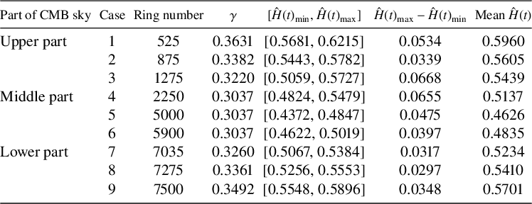
First, three CMB pixels “552300”, “1533000”, “3253800” located in the corresponding upper part rings 525, 875 and 1275 were chosen. Then for each CMB pixel in these half rings, their corresponding estimated Hölder exponents $\hat {H}(t)$
were computed. Next, another three pixels “10047488”, “32575488”, “39948288” were chosen in the middle part of the CMB sky sphere. Their ring numbers were 2250, 5000 and 5900, respectively. Finally, three CMB pixels “47656664”, “48651704”, “49375304” belonging to the lower part rings, 7035, 7275 and 7500 were selected and the pointwise Hölder exponents of pixels in their rim segments were estimated.
$\hat {H}(t)$
were computed. Next, another three pixels “10047488”, “32575488”, “39948288” were chosen in the middle part of the CMB sky sphere. Their ring numbers were 2250, 5000 and 5900, respectively. Finally, three CMB pixels “47656664”, “48651704”, “49375304” belonging to the lower part rings, 7035, 7275 and 7500 were selected and the pointwise Hölder exponents of pixels in their rim segments were estimated.
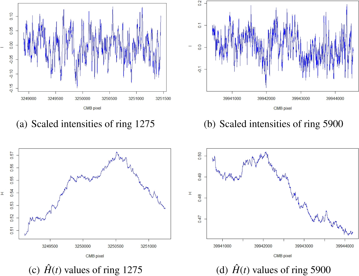
For example, Figure 2 shows the plots of the scaled intensities and the estimated pointwise Hölder exponents of the rim segments of rings 1275 and 5900, which belong to the upper and middle parts of the CMB sky sphere, respectively. It can be seen from Figures 2(a) and 2(b) that the majority of scaled intensities fall into the range $[-0.2, 0.2]$
and their fluctuations are random. Figures 2(c) and 2(d) show that the
$[-0.2, 0.2]$
and their fluctuations are random. Figures 2(c) and 2(d) show that the $\hat {H}(t)$
values in both rim sections are changing and the dispersion range for ring 1275 is wider than that of ring 5900. Similar plots and results were also obtained for other rings.
$\hat {H}(t)$
values in both rim sections are changing and the dispersion range for ring 1275 is wider than that of ring 5900. Similar plots and results were also obtained for other rings.
Examples of scaled intensities and $\hat {H}(t)$
values for one-dimensional CMB regions.
$\hat {H}(t)$
values for one-dimensional CMB regions.
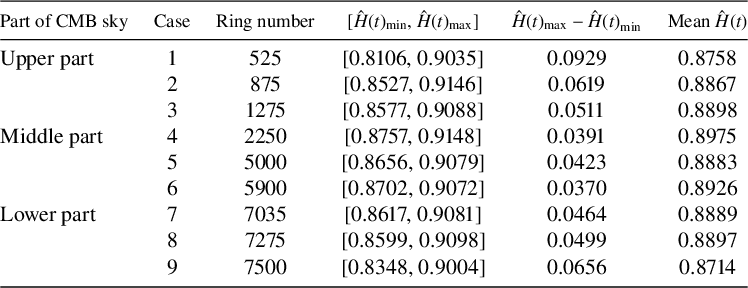
The summary of the estimated pointwise Hölder exponent values obtained by the discussed methodology is shown in Table 1. It is clear that the dispersion range of the $\hat {H}(t)$
values and the mean
$\hat {H}(t)$
values and the mean $\hat {H}(t)$
value change with ring numbers. These results suggest that the pointwise Hölder exponent values change from location to location. The summary of the estimated pointwise Hölder exponent values obtained by the conventional (R/S) method using the command RoverS from the R package fractal is given in Table 2. Note that the dispersion range and the mean
$\hat {H}(t)$
value change with ring numbers. These results suggest that the pointwise Hölder exponent values change from location to location. The summary of the estimated pointwise Hölder exponent values obtained by the conventional (R/S) method using the command RoverS from the R package fractal is given in Table 2. Note that the dispersion range and the mean $\hat {H}(t)$
value change with the spiralling ring number. Similar results were also obtained for other available estimators of the Hölder exponent. Although these numerical values are inconsistent between different methods, they all suggest that the pointwise Hölder exponent values change from location to location.
$\hat {H}(t)$
value change with the spiralling ring number. Similar results were also obtained for other available estimators of the Hölder exponent. Although these numerical values are inconsistent between different methods, they all suggest that the pointwise Hölder exponent values change from location to location.
Summary of $\hat {H}(t)$
values for pixels in different rings of the CMB sky sphere.
$\hat {H}(t)$
values for pixels in different rings of the CMB sky sphere.
Summary of $\hat {H}(t)$
values for pixels in different rings of the CMB sky sphere using the R/S method.
$\hat {H}(t)$
values for pixels in different rings of the CMB sky sphere using the R/S method.
It is expected that temperature intensities are positively dependent/correlated in close regions; see the covariance analysis in [Reference Broadbridge, Kolesnik, Leonenko and Olenko13]. Therefore, running standard equality-of-means tests under independence assumptions will provide even more significant results if the hypothesis of equal means is rejected.
To prove that distributions of $\hat {H}(t)$
are statistically different between different sky regions, we carried out several equality-of-means tests. Before that, the Shapiro test was used to ensure that the
$\hat {H}(t)$
are statistically different between different sky regions, we carried out several equality-of-means tests. Before that, the Shapiro test was used to ensure that the $\hat {H}(t)$
values satisfy the normality assumption. For all the cases considered in Table 1, their
$\hat {H}(t)$
values satisfy the normality assumption. For all the cases considered in Table 1, their $\hat {H}(t)$
values failed the normality assumption. Since the CMB pixels close to each other can be dependent, to get more reliable results, we chose CMB pixels at distance 50 apart on a ring. The Shapiro test confirmed that in all the considered upper and lower part cases in Table 1,
$\hat {H}(t)$
values failed the normality assumption. Since the CMB pixels close to each other can be dependent, to get more reliable results, we chose CMB pixels at distance 50 apart on a ring. The Shapiro test confirmed that in all the considered upper and lower part cases in Table 1, $\hat {H}(t)$
values at step 50 satisfied the normality assumption, whereas the
$\hat {H}(t)$
values at step 50 satisfied the normality assumption, whereas the $\hat {H}(t)$
values in the middle part failed the normality assumption.
$\hat {H}(t)$
values in the middle part failed the normality assumption.
Let $\mu _1$
and
$\mu _1$
and $\mu _2$
be the
$\mu _2$
be the $\text {mean}{({\hat {H}(t)})}$
values of the rim segments of rings 525 and 1275, respectively. To test the hypothesis
$\text {mean}{({\hat {H}(t)})}$
values of the rim segments of rings 525 and 1275, respectively. To test the hypothesis $H_0: \mu _1 = \mu _2$
against
$H_0: \mu _1 = \mu _2$
against $H_1: \mu _1 \neq \mu _2$
, we carried out the Wilcoxon test. The obtained p-value (
$H_1: \mu _1 \neq \mu _2$
, we carried out the Wilcoxon test. The obtained p-value (
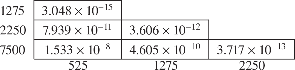
 $3.048 \times 10^{-15}$
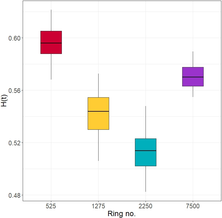
) is significantly less than 0.05 and suggests that the means are different at the 5% level of significance. Similar results were obtained for the Wilcoxon tests between all pairs of the cases in Table 1. For example, Table 3 shows Wilcoxon test results for selected four rings, two in the upper part, and the other two correspondingly in the middle and lower parts of the CMB sky sphere. Figure 3 shows the distribution box plots of the
$3.048 \times 10^{-15}$
) is significantly less than 0.05 and suggests that the means are different at the 5% level of significance. Similar results were obtained for the Wilcoxon tests between all pairs of the cases in Table 1. For example, Table 3 shows Wilcoxon test results for selected four rings, two in the upper part, and the other two correspondingly in the middle and lower parts of the CMB sky sphere. Figure 3 shows the distribution box plots of the $\hat {H}(t)$
values in the rim segments of rings 525, 1275, 2250 and 7500. It is clear from Figure 3 that the
$\hat {H}(t)$
values in the rim segments of rings 525, 1275, 2250 and 7500. It is clear from Figure 3 that the $\text {mean}{({\hat {H}(t)})}$
values are different from each other in these cases.
$\text {mean}{({\hat {H}(t)})}$
values are different from each other in these cases.
The p-values for Wilcoxon tests between different rings.
The distribution of $\hat {H}(t)$
values of four rim segments.
$\hat {H}(t)$
values of four rim segments.
Analogously to Table 3, for all Wilcoxon tests between the rim sectors in the upper, middle and lower parts, $p>0.05$
. Therefore, there is enough statistical evidence to suggest that the pointwise Hölder exponents change from location to location. While we compared Hölder exponents for different rings, from Figure 2 it is clear that
$p>0.05$
. Therefore, there is enough statistical evidence to suggest that the pointwise Hölder exponents change from location to location. While we compared Hölder exponents for different rings, from Figure 2 it is clear that $\hat {H}(t)$
is also changing for pixels within the same rings.
$\hat {H}(t)$
is also changing for pixels within the same rings.
6.2 Estimates of Hölder exponent for two-dimensional CMB regions
For two-dimensional sky regions, pointwise Hölder exponent values $H(t)$
were estimated according to equation (4.3) with
$H(t)$
were estimated according to equation (4.3) with $d=2$
, where
$d=2$
, where $V_{N}^{(2)}(t)$
was computed using equation (4.2). Equation (4.2) in Definition 4.3 can be written in the following explicit form:
$V_{N}^{(2)}(t)$
was computed using equation (4.2). Equation (4.2) in Definition 4.3 can be written in the following explicit form:
 $$ \begin{align*} V_{N}^{(2)}(t) = &\sum_{p \in v_{N}(t)}\bigg\{\sum_{k_1 \in \{0,1,2\}} \sum_{k_2 \in \{0,1,2\}} e_{k_1}e_{k_2} X\bigg(\frac{p_1+k_1}{N},\frac{p_2+k_2}{N}\bigg)\bigg\}^2 \\ =& \sum_{p \in v_{N}(t)} \bigg\{X\bigg(\frac{p_1}{N},\frac{p_2}{N}\bigg) - 2X\bigg(\frac{p_1}{N},\frac{p_2+1}{N}\bigg) -2 X\bigg(\frac{p_1+1}{N},\frac{p_2}{N}\bigg) \\ &\quad +X\bigg(\frac{p_1}{N},\frac{p_2+2}{N}\bigg) + X\bigg(\frac{p_1+2}{N},\frac{p_2}{N}\bigg) + 4 X\bigg(\frac{p_1+1}{N},\frac{p_2+1}{N}\bigg) \\ &\quad - 2 X\bigg(\frac{p_1+1}{N},\frac{p_2+2}{N}\bigg) - 2 X\bigg(\frac{p_1+2}{N},\frac{p_2+1}{N}\bigg) + X\bigg(\frac{p_1+2}{N},\frac{p_2+2}{N}\bigg)\bigg\}^2. \end{align*} $$
To compute quadratic increments of spherical random fields, relatively small parts of the sphere can be approximately considered as regions of the plane and the above formula can be applied. Note that the internal summation set $\{ ( {(p_1 + k_1)/N}, {(p_2 + k_2)/N})\mid k_1, k_2 \in \{0, 1, 2\} \}$
can be very efficiently represented by the HEALPix nested structure. Indeed, all pixels have either seven or eight neighbours (see Figure 4). The
$\{ ( {(p_1 + k_1)/N}, {(p_2 + k_2)/N})\mid k_1, k_2 \in \{0, 1, 2\} \}$
can be very efficiently represented by the HEALPix nested structure. Indeed, all pixels have either seven or eight neighbours (see Figure 4). The $3 \times 3$
configuration with eight neighbours perfectly matches the internal summation set and can be directly used in computations of
$3 \times 3$
configuration with eight neighbours perfectly matches the internal summation set and can be directly used in computations of $V_N^2(t)$
. For the case of seven neighbours, an additional eighth neighbour, the intensity of which equals to that of its adjusted pixel, was imputed. For the resolution
$V_N^2(t)$
. For the case of seven neighbours, an additional eighth neighbour, the intensity of which equals to that of its adjusted pixel, was imputed. For the resolution $N_{\text {side}} = 2048$
only 24 out of 50 331 648 pixels have seven neighbours. For such a small number of pixels, the imputation has a negligible impact on the results.
$N_{\text {side}} = 2048$
only 24 out of 50 331 648 pixels have seven neighbours. For such a small number of pixels, the imputation has a negligible impact on the results.
Examples of pixels with seven and eight neighbours for $N_{\text {side}}=4$
.
$N_{\text {side}}=4$
.
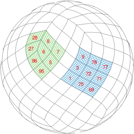
Circular regions with radius $R=0.23$
were used in the computations in this section. Let N denote the number of pixels within such circular regions. Then,
$R=0.23$
were used in the computations in this section. Let N denote the number of pixels within such circular regions. Then, $N \approx 662\, 700$
pixels. To reduce the computation time, we chose a grid of 1000 CMB pixels with step
$N \approx 662\, 700$
pixels. To reduce the computation time, we chose a grid of 1000 CMB pixels with step $662 = [662\,700/1000]$
, where
$662 = [662\,700/1000]$
, where $[\cdot ]$
denotes the integer part, over the total number of pixels. To compute local estimators
$[\cdot ]$
denotes the integer part, over the total number of pixels. To compute local estimators $\hat {H}(t)$
, for each chosen CMB pixel, a circular window with radius
$\hat {H}(t)$
, for each chosen CMB pixel, a circular window with radius $r=0.01$
was selected. The value of
$r=0.01$
was selected. The value of $\gamma $
was computed as
$\gamma $
was computed as $\gamma ={- (\log (\sqrt {\pi }r/2)/\!\log (\sqrt {N}))}$
for given values of N and r. The factor
$\gamma ={- (\log (\sqrt {\pi }r/2)/\!\log (\sqrt {N}))}$
for given values of N and r. The factor $\sqrt {\pi }/2$
appeared as the number of pixels is proportional to a window area. To match the number of pixels in circular window regions that were used in computations and square regions used for summation in
$\sqrt {\pi }/2$
appeared as the number of pixels is proportional to a window area. To match the number of pixels in circular window regions that were used in computations and square regions used for summation in $V_{N}^{(2)}(t)$
, the length
$V_{N}^{(2)}(t)$
, the length $2{d_0}$
of the side of squares should satisfy the equation
$2{d_0}$
of the side of squares should satisfy the equation ${(2{d_0})^2} = {\pi r^2}$
. The
${(2{d_0})^2} = {\pi r^2}$
. The $\gamma $
obtained was substituted in equation (4.3) to compute the estimated pointwise Hölder exponent values. For
$\gamma $
obtained was substituted in equation (4.3) to compute the estimated pointwise Hölder exponent values. For $r=0.01$
, there are approximately 2836 pixels in each specified window. For each of these pixels, the squared increment was computed and the total of increments was obtained by the expression for
$r=0.01$
, there are approximately 2836 pixels in each specified window. For each of these pixels, the squared increment was computed and the total of increments was obtained by the expression for $V_{N}^{(2)}(t)$
.
$V_{N}^{(2)}(t)$
.
Initially, the two-dimensional regions were selected randomly. Then, from those candidates, regions with majority warm, majority cold, a mixture of temperatures, and borderline regions were selected. The paper presents only results about those selected regions. Similar results were obtained for other analogous regions, but, due to space restrictions, are not given here.
First, a circular CMB sky window of radius $R=0.23$
from a warm area with a majority of high temperature intensities was selected. The mean temperature intensity in the selected CMB sky region covering the warm area was
$R=0.23$
from a warm area with a majority of high temperature intensities was selected. The mean temperature intensity in the selected CMB sky region covering the warm area was $5.978\,61 \times 10^{-5}$
. The window is shown in Figure 5(a). The number of pixels in that specific window was 662 685. Then different circular CMB sky windows having a radius of
$5.978\,61 \times 10^{-5}$
. The window is shown in Figure 5(a). The number of pixels in that specific window was 662 685. Then different circular CMB sky windows having a radius of $R=0.23$
covering cold, mixture, and borderline regions shown in Figures 5(b), 5(c) and 5(d) were chosen. In each of the cold, mixture of warm and cold and a borderline having warm and cold regions, the number of pixels were 662 697, 662 706 and 662 725, respectively. The value of
$R=0.23$
covering cold, mixture, and borderline regions shown in Figures 5(b), 5(c) and 5(d) were chosen. In each of the cold, mixture of warm and cold and a borderline having warm and cold regions, the number of pixels were 662 697, 662 706 and 662 725, respectively. The value of $\gamma $
was computed as
$\gamma $
was computed as $\gamma =0.705$
for each CMB sky region. The corresponding mean temperature intensities were
$\gamma =0.705$
for each CMB sky region. The corresponding mean temperature intensities were $-8.340\,55 \times 10^{-5}$
,
$-8.340\,55 \times 10^{-5}$
, $-1.740\,35 \times 10^{-5}$
and
$-1.740\,35 \times 10^{-5}$
and $7.598\,51 \times 10^{-6}$
.
$7.598\,51 \times 10^{-6}$
.
Sky windows used for computations.
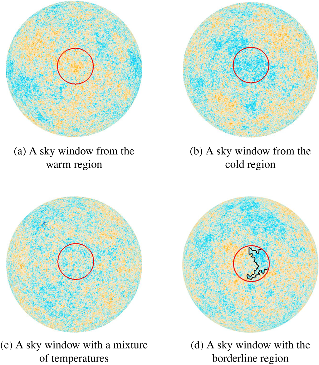
The plots of the estimated pointwise Hölder exponent values for each case are displayed in Figure 6. These $\hat {H}(t)$
values are mostly dispersed in the interval
$\hat {H}(t)$
values are mostly dispersed in the interval $[0.36, 0.86]$
. Figure 6 shows an erratic and an irregular behaviour in the distribution of
$[0.36, 0.86]$
. Figure 6 shows an erratic and an irregular behaviour in the distribution of $\hat {H}(t)$
values. It can be observed that the estimates in Figures 6(a) and 6(d) with substantial warm temperatures have larger
$\hat {H}(t)$
values. It can be observed that the estimates in Figures 6(a) and 6(d) with substantial warm temperatures have larger $\hat {H}(t)$
fluctuations than the
$\hat {H}(t)$
fluctuations than the $\hat {H}(t)$
values for cold regions.
$\hat {H}(t)$
values for cold regions.
Local estimates $\hat {H}(t)$
for two-dimensional regions.
$\hat {H}(t)$
for two-dimensional regions.

The summary of the estimated pointwise Hölder exponents for each selected region is given in Table 4. It shows the mean CMB temperature intensities of each circular window. Table 4 also presents the estimated minimum, maximum and mean $\hat {H}(t)$
values computed by using the selected 1000 CMB pixels. It is clear from this table that the mean
$\hat {H}(t)$
values computed by using the selected 1000 CMB pixels. It is clear from this table that the mean $\hat {H}(t)$
value from the warm region is the highest and it is the lowest for the borderline region. The mean
$\hat {H}(t)$
value from the warm region is the highest and it is the lowest for the borderline region. The mean $\hat {H}(t)$
values of the cold region and mixture case lie in between. It is apparent from Table 4 that the range of the estimated pointwise Hölder exponent values changes with respect to the temperature of the chosen regions of the CMB sky sphere.
$\hat {H}(t)$
values of the cold region and mixture case lie in between. It is apparent from Table 4 that the range of the estimated pointwise Hölder exponent values changes with respect to the temperature of the chosen regions of the CMB sky sphere.
To further investigate the estimated pointwise Hölder exponents, they were computed for 100 random CMB pixels in each of the regions considered. It was apparent that even if one accounts for variation by considering these 100 CMB pixels, the $\hat {H}(t)$
values between different regions are different. The analyses suggested that all
$\hat {H}(t)$
values between different regions are different. The analyses suggested that all $\hat {H}(t)$
values for 100 and 1000 CMB pixels were consistent. Therefore, the results suggest that the estimated pointwise Hölder exponent values change from place to place.
$\hat {H}(t)$
values for 100 and 1000 CMB pixels were consistent. Therefore, the results suggest that the estimated pointwise Hölder exponent values change from place to place.
To prove that $\hat {H}(t)$
is significantly different between different sky windows, we carried out several equality-of-means tests. Initially, we carried out the Shapiro test to ensure that the
$\hat {H}(t)$
is significantly different between different sky windows, we carried out several equality-of-means tests. Initially, we carried out the Shapiro test to ensure that the $\hat {H}(t)$
values satisfy the normality assumption. However, for all the cases considered in Table 4, their
$\hat {H}(t)$
values satisfy the normality assumption. However, for all the cases considered in Table 4, their $\hat {H}(t)$
values failed the normality assumption. Figure 7 displays the distribution box plots of the
$\hat {H}(t)$
values failed the normality assumption. Figure 7 displays the distribution box plots of the $\hat {H}(t)$
values in the CMB sky windows with warm, cold, mixture and borderline regions. It can be observed from Figure 7 that the
$\hat {H}(t)$
values in the CMB sky windows with warm, cold, mixture and borderline regions. It can be observed from Figure 7 that the $\hat {H}(t)$
distributions have extreme values in all four cases. Thus, we present only results from the Wilcoxon test as it is reliable amidst the nonnormality of data and in the presence of outliers.
$\hat {H}(t)$
distributions have extreme values in all four cases. Thus, we present only results from the Wilcoxon test as it is reliable amidst the nonnormality of data and in the presence of outliers.
Let $\mu _1$
and
$\mu _1$
and $\mu _2$
be the
$\mu _2$
be the $\text {mean}{({\hat {H}(t)})}$
values in the sky windows with warm and cold regions, respectively. Testing the hypothesis
$\text {mean}{({\hat {H}(t)})}$
values in the sky windows with warm and cold regions, respectively. Testing the hypothesis $H_0: \mu _1 = \mu _2$
against
$H_0: \mu _1 = \mu _2$
against $H_1: \mu _1 \neq \mu _2$
using a Wilcoxon test, we obtained
$H_1: \mu _1 \neq \mu _2$
using a Wilcoxon test, we obtained $p <2.2 \times 10^{-16}$
, highly significant at the 5% level. It suggests that the means are different at 5% level of significance. Similar results were obtained for the Wilcoxon tests between all pairs of the cases, and the corresponding p-values are shown in Table 5. This suggests that the
$p <2.2 \times 10^{-16}$
, highly significant at the 5% level. It suggests that the means are different at 5% level of significance. Similar results were obtained for the Wilcoxon tests between all pairs of the cases, and the corresponding p-values are shown in Table 5. This suggests that the $\text {mean}{({\hat {H}(t)})}$
values are different from each other in all the cases. Apart from variations between the cases, we observe from Figure 6 and Table 4 that the estimated Hölder exponents do change within individual sky windows as well.
$\text {mean}{({\hat {H}(t)})}$
values are different from each other in all the cases. Apart from variations between the cases, we observe from Figure 6 and Table 4 that the estimated Hölder exponents do change within individual sky windows as well.
Analysis of CMB sky windows with different temperatures.
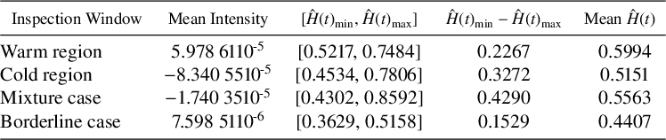
The distribution of $\hat {H}(t)$
values for chosen sky windows.
$\hat {H}(t)$
values for chosen sky windows.
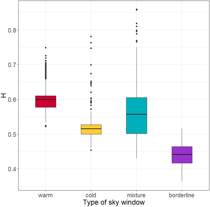
The p-values for Wilcoxon tests between chosen sky windows.
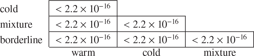
Therefore, there is enough evidence to suggest that the pointwise Hölder exponents change from location to location of the CMB sky sphere.
6.3 Analysis of CMB temperature anomalies
As previously discussed in Section 1, several missions have measured the CMB temperature anisotropies, gradually increasing their precision by using advanced radio telescopes. This section discusses applications of the multifractional methodology to detect regions of CMB maps with “anomalies”. In particular, it can help in evaluating various reconstruction methods for blocked regions with unavailable or too noisy data.
It is well known that the CMB maps are affected by interference from the Milky Way, and radio signals emitting from our galaxy are much noisier than the CMB. Thus, the Milky Way blocks the CMB near the galactic plane. However, the smooth and predictable nature of Milky Way’s radiation spectrum has enabled the cosmological attributes to be found by subtracting the spectrum from the initially observed intensities [Reference Castelvecchi16]. From Planck 2015 results, the CMB maps have been cleaned and reconstructed using different techniques namely, COMMANDER, NILC, SEVEM and SMICA (see [Reference Ade3] for more information). We are using the CMB map produced from the SMICA method [23] with $N_{\text {side}}=2048.$
To examine the random behaviour of isotropic Gaussian fields on the sphere, a direction-dependent mathematical tool has been proposed in [Reference Hamann, Gia, Sloan, Wang and Womersley21]. The authors applied their probe to investigate the CMB maps from Planck PR2 2015 and PR3 2018 with specific consideration of cosmological data from the inpainted maps. To detect departures from the traditional stochastic model of the CMB data, they utilized the autocorrelation of the sequence of full-sky Fourier coefficients and have proposed an “AC discrepancy” function on the sphere. For the inpainted Planck 2015 COMMANDER map, [Reference Hamann, Gia, Sloan, Wang and Womersley21] shows the maximum “AC discrepancy” for the galactic coordinates, $(l,b) = (353.54, 1.79)$
. Similarly, for the inpainted Planck COMMANDER 2018, NILC 2018, SEVEM 2018 and SMICA 2018 with
$(l,b) = (353.54, 1.79)$
. Similarly, for the inpainted Planck COMMANDER 2018, NILC 2018, SEVEM 2018 and SMICA 2018 with $N_{\text {side}}=1024$
, there are significant departures at the galactic coordinates (12.57, 0.11),
$N_{\text {side}}=1024$
, there are significant departures at the galactic coordinates (12.57, 0.11), $(61.17,-30.73)$
,
$(61.17,-30.73)$
, $(261.25,-2.99)$
and
$(261.25,-2.99)$
and $(261.34,-2.99)$
, respectively. A majority of these locations are the masked regions of the galactic plane. The galactic coordinates corresponding to the largest deviations are different for each map depicting the discrepancies in the underlying inpainting techniques.
$(261.34,-2.99)$
, respectively. A majority of these locations are the masked regions of the galactic plane. The galactic coordinates corresponding to the largest deviations are different for each map depicting the discrepancies in the underlying inpainting techniques.
The approach of Hamann et al. [Reference Hamann, Gia, Sloan, Wang and Womersley21] used directional dependencies in CMB data on the unit sphere. The results below are based on a different approach that uses the local roughness properties of these data. Therefore, the detected regions of high anomalies can be different for these two methods as they reflect different physical anisotropic properties of CMB (see, for example, Figure 10). The estimated local Hölder exponents on one-dimensional rings can be considered as directional local probes of CMB anisotropy. However, the estimates for two-dimensional regions are more complex and aggregate local information about roughness in different directions.
In the following analysis, we use estimated values of the Hölder exponent to detect regions of possible anomalies in CMB maps. Figure 8 shows the plots of scaled intensities and estimated Hölder exponent values $\hat {H}(t)$
in one- and two-dimensional CMB regions of the great circle. We notice from Figure 8(a) that there is an increase in the fluctuations of the scaled intensity values between the HEALPix range
$\hat {H}(t)$
in one- and two-dimensional CMB regions of the great circle. We notice from Figure 8(a) that there is an increase in the fluctuations of the scaled intensity values between the HEALPix range $[25\,163\,000, 25\,164\,000]$
of the great circle ring. A low plateau of estimated
$[25\,163\,000, 25\,164\,000]$
of the great circle ring. A low plateau of estimated $\hat {H}(t)$
values in Figure 8(b) corresponds to that range of HEALPix values. The equator rim segment with the unusual plateau of
$\hat {H}(t)$
values in Figure 8(b) corresponds to that range of HEALPix values. The equator rim segment with the unusual plateau of $\hat {H}(t)$
values has CMB pixel numbers ranging from 25 163 208 to 25 163 852. Their corresponding galactic coordinates were found to be between,
$\hat {H}(t)$
values has CMB pixel numbers ranging from 25 163 208 to 25 163 852. Their corresponding galactic coordinates were found to be between, $(65.02, 0.01)$
and
$(65.02, 0.01)$
and $(93.32, 0.01)$
.
$(93.32, 0.01)$
.
Scaled intensities and estimated $\hat {H}(t)$
values in one- and two-dimensional regions of the great circle.
$\hat {H}(t)$
values in one- and two-dimensional regions of the great circle.
Similarly, this unusual behaviour of $\hat {H}(t)$
values was observed in the two-dimensional CMB regions near the galactic plane/equator. Figure 8(c) shows the plot of scaled intensities in the two-dimensional space and a spike in intensities can be observed near the specified range of HEALPix values. The corresponding lower valley of
$\hat {H}(t)$
values was observed in the two-dimensional CMB regions near the galactic plane/equator. Figure 8(c) shows the plot of scaled intensities in the two-dimensional space and a spike in intensities can be observed near the specified range of HEALPix values. The corresponding lower valley of $\hat {H}(t)$
values can be seen in Figure 8(d). The four corners of the spherical region having unusual
$\hat {H}(t)$
values can be seen in Figure 8(d). The four corners of the spherical region having unusual $\hat {H}(t)$
values have HEALPix values 23 404 309, 23 391 936, 23 564 929 and 24 158 424. Their galactic coordinates were found as
$\hat {H}(t)$
values have HEALPix values 23 404 309, 23 391 936, 23 564 929 and 24 158 424. Their galactic coordinates were found as $(85.91, -1.66)$
,
$(85.91, -1.66)$
, $(76.82, -1.66)$
,
$(76.82, -1.66)$
, $(76.82, 4.05)$
and
$(76.82, 4.05)$
and $(85.91, 4.05)$
, respectively.
$(85.91, 4.05)$
, respectively.
Table 6 shows the summary of CMB intensities at these one- and two-dimensional equatorial regions. The two-dimensional region around the unusual values was extracted as a rectangular spherical region from the circular CMB window using the previously identified galactic coordinates to split them as the unusual and the remaining regions. It is clear that the range of temperature intensities is wider in the one- and two-dimensional regions around the unusual values than in the regions excluding them. Further, the variances of intensities in the anomalous regions are larger than in the remaining regions. Moreover, Table 6 confirms that the mean $\hat {H}(t)$
values in the anomalous regions are lower than in the remaining regions.
$\hat {H}(t)$
values in the anomalous regions are lower than in the remaining regions.
Analysis of CMB intensities near the equatorial region.
Figure 9 shows the Planck 2015 map with blocked nonreliable CMB values. The region of CMB values where the TMASK is applied by the SMICA reconstruction technique, is removed in Figure 9. The TMASK of the CMB intensities utilized by the SMICA method determines the region where the inpainted CMB intensities in the galactic plane are considered to be reliable. The rectangular window shows a possible region of anomalies detected by the developed multifractional methodology.
SMICA 2015 map with TMASK and the region of anomalies.

We now apply this approach and investigate $\hat {H}(t)$
for all
$\hat {H}(t)$
for all $t \in s_2(1)$
. First, the one-dimensional methodology was used.
$t \in s_2(1)$
. First, the one-dimensional methodology was used. $\hat {H}(t)$
was estimated using the CMB intensities on rims, similar to the analysis in Figures 8(a) and 8(b). The moving windows with 4096 consecutive pixels, which is approximately half of a full ring, were used to obtain values of
$\hat {H}(t)$
was estimated using the CMB intensities on rims, similar to the analysis in Figures 8(a) and 8(b). The moving windows with 4096 consecutive pixels, which is approximately half of a full ring, were used to obtain values of $\hat {H}(t)$
. To clearly show local behaviours, after several trials, sets
$\hat {H}(t)$
. To clearly show local behaviours, after several trials, sets $v_N(t)$
with 61 HEALPix points, that is, where the radius equals 30 pixels, were selected. The results obtained are shown in Figure 10(a). To compare them with the AC discrepancy approach in [Reference Hamann, Gia, Sloan, Wang and Womersley21], Figure 10(b) shows the corresponding map obtained by applying the direction-dependent probe. The code from [Reference Wang44] was used to compute values of AC discrepancies for SMICA 2015 CMB intensities. The first map highlights
$v_N(t)$
with 61 HEALPix points, that is, where the radius equals 30 pixels, were selected. The results obtained are shown in Figure 10(a). To compare them with the AC discrepancy approach in [Reference Hamann, Gia, Sloan, Wang and Womersley21], Figure 10(b) shows the corresponding map obtained by applying the direction-dependent probe. The code from [Reference Wang44] was used to compute values of AC discrepancies for SMICA 2015 CMB intensities. The first map highlights $\hat {H}(t)$
values below the
$\hat {H}(t)$
values below the $5$
th percentile. AC discrepancy values above the
$5$
th percentile. AC discrepancy values above the ${95}^{}$
th percentile were used for the second map. Both approaches detected the region of anomalies in Figure 9. However, from locations of other discrepancy values, it is clear that these approaches detect different CMB anomalies.
${95}^{}$
th percentile were used for the second map. Both approaches detected the region of anomalies in Figure 9. However, from locations of other discrepancy values, it is clear that these approaches detect different CMB anomalies.
Discrepancy maps for CMB intensities from SMICA 2015.
Very sharp changes in $\hat {H}(t)$
values in Figure 8(b) motivated the second method to detect anomalies, which is based on increments of
$\hat {H}(t)$
values in Figure 8(b) motivated the second method to detect anomalies, which is based on increments of $\hat {H}(t)$
values. Figure 8(b) demonstrated substantial changes of
$\hat {H}(t)$
values. Figure 8(b) demonstrated substantial changes of $\hat {H}(t)$
for nearby t locations. These changes are permanent as
$\hat {H}(t)$
for nearby t locations. These changes are permanent as $\hat {H}(t)$
exhibits stable behaviour after a rapid “jump”. Such changes are different from noise or outliers, when values in random distinct locations lie at an abnormal distance from other values in their surrounding points.
$\hat {H}(t)$
exhibits stable behaviour after a rapid “jump”. Such changes are different from noise or outliers, when values in random distinct locations lie at an abnormal distance from other values in their surrounding points.
To detect such rapid changes, we used the statistics ${\hat {H}}_{\Delta }(t) = \min _{t_1 \in {\Delta }{(t)}}\lvert {\hat {H}}(t)-{\hat {H}}(t_1)\rvert $
, where t and
${\hat {H}}_{\Delta }(t) = \min _{t_1 \in {\Delta }{(t)}}\lvert {\hat {H}}(t)-{\hat {H}}(t_1)\rvert $
, where t and $t_1$
are indices of ring-ordered pixels and the set
$t_1$
are indices of ring-ordered pixels and the set $\Delta {(t)}$
=
$\Delta {(t)}$
= $\{t+10,\ldots ,t+20\}$
. The delay of 10 was selected to detect jumps that occur over short distances. The minimum over the set of consecutive points
$\{t+10,\ldots ,t+20\}$
. The delay of 10 was selected to detect jumps that occur over short distances. The minimum over the set of consecutive points $\Delta {(t)}$
was used to eliminate outliers or noise that can result in distinct large differences
$\Delta {(t)}$
was used to eliminate outliers or noise that can result in distinct large differences $\lvert {\hat {H}}(t)-{\hat {H}}(t_1)\rvert $
.
$\lvert {\hat {H}}(t)-{\hat {H}}(t_1)\rvert $
.
Figure 11(a) shows the computed ${\hat {H}}_{\Delta }(t)$
values for SMICA 2015 CMB intensities. Here,
${\hat {H}}_{\Delta }(t)$
values for SMICA 2015 CMB intensities. Here, ${\hat {H}}_{\Delta }(t)$
values above the
${\hat {H}}_{\Delta }(t)$
values above the ${95}$
th percentile are plotted.
${95}$
th percentile are plotted. ${\hat {H}}_{\Delta }$
discrepancy maps for CMB intensities from SMICA 2015.
${\hat {H}}_{\Delta }$
discrepancy maps for CMB intensities from SMICA 2015.

It is well known that the galactic centre and equatorial region are the most problematic and questionable areas of the CMB maps. Our methodology classified the galactic centre as anomalous based on its Hölder exponent value above the 95th percentile. The contextualization has been already provided by Hamann et al. [Reference Hamann, Gia, Sloan, Wang and Womersley21]; it is due to difficulties in producing correct cleaned CMB maps in this region.
In Figure 11(b), $5\%$
of largest
$5\%$
of largest ${\hat {H}}_{\Delta }(t)$
values are shown on the TMASK map. Note that in most cases, clusters of largest
${\hat {H}}_{\Delta }(t)$
values are shown on the TMASK map. Note that in most cases, clusters of largest ${\hat {H}}_{\Delta }(t)$
values are within the TMASK. It seems that
${\hat {H}}_{\Delta }(t)$
values are within the TMASK. It seems that ${\hat {H}}_{\Delta }$
indices rather accurately detected many regions with unreliable CMB values. Analysis of other CMB maps gave similar results.
${\hat {H}}_{\Delta }$
indices rather accurately detected many regions with unreliable CMB values. Analysis of other CMB maps gave similar results.
Summarizing, the methodology implemented to investigate multifractional presence within the CMB temperature intensities could also serve as a mechanism to detect regions of anomalies in CMB maps.
7 Conclusion
In this paper, we examined multifractional spherical random fields and their application to analysis of cosmological data from the Planck mission. The paper developed the general methodology for estimation of pointwise Hölder exponents of multifractional data observed on the unit sphere. It estimated pointwise Hölder exponent values for the actual CMB temperature intensities and checked for the presence of multifractionality. The estimators of pointwise Hölder exponents for one- and two-dimensional regions were obtained by using the ring and nested orderings of the HEALPix visualization structure. The analysis carried out conveyed multifractionality in the CMB temperature intensities, since the computed pointwise Hölder exponent values do substantially change from place to place in the CMB sky sphere. The proposed method was used for numerical studies of the CMB data and found anisotropies in the temperature intensities. In particular, validity and usefulness of the method were evidenced by detecting numerous anisotropies in unreliable CMB regions of the TMASK.
The approach developed and the computing techniques implemented can also be used for other types of spherical data, such as solar data, planetary data, meteorological data, pollution data and earth data. First, the R package rcosmo [Reference Fryer, Li and Olenko18] can be used to transform spherical data into the HEALPix format. Then the methods developed can be directly applied by using the publicly available R code for this paper.
Some numerical approaches that were used to speed up computations for big CMB data sets will be reported in future publications. In future studies, it would be also interesting to:
-
• develop the distribution theory for the estimators of $H(t)$
;
$H(t)$
; -
• investigate reliability and accuracy of various estimators of the Hölder exponent for the CMB;
-
• study rates of convergence in Theorem 4.4 (see results on superconvergence by McLean [Reference McLean35]);
-
• investigate changes of the Hölder exponents depending on evolutions of random fields driven by SPDEs on the sphere [Reference Anh, Broadbridge, Olenko and Wang5, Reference Broadbridge, Kolesnik, Leonenko and Olenko13, Reference Broadbridge, Kolesnik, Leonenko, Olenko and Omari14];
-
• study directional changes of the Hölder exponent by extending the results obtained for the conventional ring ordering to rings with arbitrary orientations;
-
• apply our methodology to other spherical data, in particular, to new high-resolution CMB data from future CMB-S4 surveys [Reference Abazajian1];
-
• explore relations between the locations of the detected CMB anomalies and other cosmic objects.

At high values of l, the signal will be weakened by Silk damping and possibly clouded by pressure variations due to turbulence within the plasma, as currently observed in stars. We feel that it is worthwhile to analyse the full signal that is currently available. Higher-resolution measurements in the future will distinguish how much of the analysis is due to physical causes or currently remaining galactic noise.
Acknowledgements
This research was partially supported under the Australian Research Council’s Discovery Projects funding scheme (project no. DP160101366). We would like to thank Prof. A. Ayache for attracting our attention to and discussing mutifractional models for random fields and Prof. I. Sloan for various discussions about mathematical modelling of CMB data. The authors are also grateful to the referees for their suggestions that helped to improve the style of the paper.
This research includes computations using the Linux computational cluster Gadi of the National Computational Infrastructure (NCI), which is supported by the Australian Government and La Trobe University. We are also grateful for the use of data on the Planck/ESA mission from the Planck Legacy Archive.


 Open access