

Introduction
Theoretical studies during the past 15 years have contributed significantly to our understanding of the internal and subglacial parts of a temperate glacier‘s drainage system, Reference NyeNye (1953) analyzed the closure of circular passages by plastic deformation and Reference HaefeliHaefeli (1970, p. 207) seems to have been among the first to mention the role of flowing water in enlarging such passages by melting. Reference RöthlisbergerRothlisberger (1972, p. 178) and Reference ShreveShreve (1972, p. 206) assumed a balance between these two processes in the steady state, and used this to develop theoretical models for water flow in such tunnels. Their models are valid only for situations in which the tunnels are completely filled with water. The pressure in the water is then just slightly less than that in the ice, the latter being proportional to the ice thickness.
Reference ShreveShreve (1972, p. 209–10) mentions briefly the possibility of unfilled passages, and Reference RöthlisbergerRöthlisberger (1972, p. 186, p. 193) encountered a few situations in which his solutions predicted the existence of such conduits. Neither author pursued this result to investigate the range of conditions under which such conduits might be expected. Reference LliboutryLliboutry (1983), however has looked at this possibility more closely, and recognizes that many passages may not be filled with water much of the time, even under steady-state conditions.
In the present paper this alternative is analyzed in greater detail. The equations developed apply only when the potential melting rate on passage walls just barely exceeds the closure rate. It is shown that this possibility may be more common than previously anticipated. This may have significant implications for glacier behavior and for the development of some common glacial landforms.
Theoretical Development
From turbulent pipe flow theory we have (Reference Hunsaker and RightmireHunsaker and Rightmire, 1947, equation 8.11)

where Pi is the water pressure at location i in a cylindrical conduit of diameter D c and friction coefficient f, which is carrying water of density ρW moving at velocity V, z i is the elevation of point i, g is the acceleration due to gravity, and L is the distance between two cross-sections, i = 1, 2 (Fig. 1). If the melt rate is slightly larger than the closure rate, the passage will be somewhat larger than necessary to carry the discharge provided. Under these conditions the pressure at the water surface in the tunnel will be atmospheric if there is a connection to the glacier surface. In the absence of such a connection, the pressure will be determined by the volume of air entrained in the water and in bubbles in the ice; if there is no trapped air, the pressure could fall to its triple-point value. In any case P2 = P1 and the first term in Equation (1) vanishes. We will refer to conduits in which this occurs as “open” whether or not there is a connection to the glacier surface.
Definition of symbols used in Equation (1).

It should be emphasized that Equation (1) applies only when the conduit is essentially full. As the air space in the tunnel increases, f will decrease and the flow will accelerate, thus further decreasing the cross-sectional area of the conduit occupied by water. In the following development we are concerned principally with defining the conditions under which the transition from a full to an open conduit may occur. No attempt is made to explore in detail the characteristics of flow in the open conduit.
From continuity relations we have Q =πVD c 2/4, where Q is the water discharge. Geometrically, (z 2−z 1)/L = sin β, Where β is the local bed slope. In accord with the coordinate system adopted in Figure 1, β is positive if the glacier bed slopes downward in the direction of flow. Making these substitutions and solving Equation (1) for D c, we obtain

As we are primarily interested in conduits at the glacier bed, a circular cross-section is unreasonable. Reference RöthlisbergerRöthlisberger (1972, p. 192) and Reference ShreveShreve (1972, p. 213.) use a semicircular cross-section in their examples, and that form is adopted here. The hydraulic radius of this semicircular passage should presumably be the same as that of a circular passage capable of carrying the same discharge, if differences in friction factor are ignored. Thus D S = ((π +2)/π )D C, where D s is the diameter of the semicircular passage. Assuming this scaling, and taking f = 0.05 as a plausible value for the friction coefficient (Reference Hunsaker and RightmireHunsaker and Rightmire, 1947, p. 127), we obtain

where the constant factor c1 has the value 0.55 s2/5m−1/5.
The potential energy released per unit time as the water falls through a vertical distance h will be ρw Qgh. In a full conduit, part of this energy may be needed to warm the water as the glacier thins and the pressure-melting temperature T m rises. However in a conduit in which the water pressure is constant, the temperature will not vary with ice thickness. On the other hand, due to the overburden pressure, ice in the walls of such a conduit will be colder than the water, so some of the energy in the water will be lost by conduction to the ice. The remainder is, however, available for melting ice at a rate ṁ, thus

where ρi is the density of ice, H is the heat of fusion, R is the distance into the wall of the tunnel, K is the thermal conductivity of ice, and p i is the pressure in the ice. If Z(x) is the glacier thickness, Reference NyeNye’s (1953) relations can be used to show that dp i/dR = 8ρi gZ/9D s on the tunnel wall. Then, noting that sin β = h/L, we obtain

With K = 2.1 J/m s deg and dT m/dpi = 9.8 × 10⁻⁸deg/Pa for air-saturated water and ice (Reference RöthlisbergerHarrison, 1972), the second term within the brackets becomes 9.1 × 10⁻⁸Z. Reference PatersonPaterson (1971) notes, however, that the thermal conductivity of ice very near the melting point is between 1% and 10% of the cold-ice value used above. In addition, the above calculations do not take into consideration the temperature rise across the tunnel wall that is necessary for a finite rate of heat transfer. In view of the very low temperature differences involved, this could easily reduce heat loss by a factor of two. Thus the second term is probably of the order 5 × 10⁻⁹Z or 5 × 10⁻¹⁰Z whereas the first is of the order 10−2 Q or higher for appreciable bed slopes. The second term can thus be neglected when the ice thickness is less than a few hundred meters and discharges exceed about 10−3 m3/s. The consequences of this assumption are explored more fully later.
Neglecting this term and eliminating D s from Equations (3) and (5) yields

with ρi = 916 kg/m3, ρW = 999.8 kg/m3 at 0°C, and H = 3.34 × 10⁵ J/kg, C 2 = 3.73 × 10⁻⁵ m−4/5s−2/5.
The closure rate ṙ of the tunnel is approximately (Reference NyeNye, 1953)

where B is the viscosity parameter in Glen’s flow law for homogeneous isotropic ice, έ = (τ/B) n . Here έ and τ are the effective strain-rate and stress, respectively. Equation (7) is strictly valid only when ρi gZ ≈ τ, and when there are no frictional forces resisting sliding over the bed in a direction normal to the tunnel axis, the first of these conditions is approximately satisfied, as ρi gZ will be a few megapascals for typical glacier thicknesses, whereas other stresses contributing to τ are on the order of 0.1 MPa. The second condition is also probably reasonable, except very close to the bed, for instantaneous deformation of an initially semicircular tunnel. Eliminating D s from Equation (3) and (7) and taking n = 3 in the flow law yields

with B = 1.6 × 10⁵ Pa a1/3 (Reference HookeHooke, 1981; Reference LliboutryLliboutry, 1983), C3 = 5.70 × 10⁻¹⁴ m−16/5 s−3/5.
From Equation (6) and (8) the condition ṁ > ṙ can then be written as

where C 4 = 6.55 × 10⁸ m12/5s1/5. When this condition obtains, the potential melt rate on the tunnel walls will exceed the closure rate and the tunnel will be larger than necessary to carry the discharge provided.
[Reference RöthlisbergerRöthlisberger’s (1972) limiting condition for applicability of his theory (his Equation (22)) is equivalent to Equation (9) above. To show this, dp/dx (= ρw g dh/dx ) in his Equation (9) is set equal to ρw g sin β, in accord with the assumptions made in the present paper, and the resulting relation or Q is then used in Equation (2) to obtain the relation k = 45/3 (g/8f)1/2/D c 1/6 between his roughness parameter k and the corresponding parameter f in the present paper. In addition, adjustment must be made or the conversion between the circular channel crosssection which he used and the semicircular shape assumed herein. Reference WeertmanWeertman’s (1972) equation (63) can be reduced to Röthlisberger’s equatiion (22), but for a small constant factor, and thus it too is essentially equivalent to Equation (9) of the present paper.]
In Figure 2, β has been plotted as a function of Q for various values of Z and for the case when Q equals the right-hand side of Equation (9). For any given combination of ice thickness and bed slope, the minimum value of Q that should lead to an open conduit can be read from this graph. For example, for a typical ice thickness of 250 m, water discharges in excess of about 0.1 m3/s on a 5° bed slope should result in open conduits. As discharges in proglacial streams are typically in excess of 1 m3/s it is clear that most of the larger subglacial conduits in valley glaciers may be "open" in areas of down-glacier sloping bed topography. Reference LliboutryLliboutry (1983) reaches a similar conclusion but from different reasoning. To the extent that water draining from the surface is above the melting point (Reference ShreveShreve, 1972), or that there is a significant contribution of such "warm" water from groundwater (Reference LliboutryLliboutry, 1983) the area of the glacier bed over which this condition obtains will be larger.
Critical values of discharge, bed slope, and ice thickness. If the discharge in a conduit is greater than the value read on the abscissa for a given bed slope and ice thickness, the conduit is likely to be open.
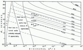
To explore further the effect of heat loss to the tunnel walls, the second term within the brackets in Equation (5) was set equal to 5 × 10⁻¹⁰ Z, and the region of Figure 2 in which this term exceeded 10% of the first term was identified as a region in which such heat loss "probably" reduces ṁ appreciably. The region in which 5 × 10⁻⁹Z exceeds 10% of the first term is likewise identified as a region in which such heat loss “may“ reduce ṁ appreciably. It is apparent that this heat loss significantly affects the conditions under which open conduits may be expected only when the discharge is quite small.
[Reference RöthlisbergerRöthlisberger (1972, p. 188) applied his theory to vertical conduits, but reached a conclusion different from that implied by Figure 2. This is because he began with the assumption ṁ = ṙ, so the resulting solution yielded conduit diameters and hence water velocities, that satisfied the energy balance implicit in ṁ = ṙ. The resulting velocities —0.5 m/s, for example, for water descending in a vertical conduit in ice with B = 1.8 × 10° Pa a1/3 —are very low, and imply some form of constriction in the outflow from the bottom of the conduit.]
Uncertainties
Reference RöthlisbergerRöthlisberger (1972, p. 182) has pointed out the substantial uncertainties in such calculations. The largest sources of error are in the values of the friction coefficient f and the flow-law viscosity parameter B. To illustrate the effect of varying these parameters within possible, but probably extreme, limits, calculations were done for Z = 250 m with B = 1.2 × 10⁵ Pa a1/3 and 2.0 × 10⁵ Pa a1/3, and with f = 0.10 and 0.025. These lines are plotted in Figure 2. It will be noted that the uncertainty in B leads to a fairly substantial uncertainty in the calculations, while that in f is much less important, a conclusion also reached by Reference RöthlisbergerRöthlisberger (1972). Softer ice (b = 1.2 × 10⁵ Pa a1/3) leads to higher closure rates, so higher discharges are required to maintain an open tunnel.
Reference LliboutryLliboutry (1983) has suggested another source of uncertainty. He notes that pressures in the ice are increased on the up-glacier sides of obstacles on the bed and decreased on the down-glacier sides of such obstacles, and that this will affect the rate of tunnel closure. Due to the non-linearity of the flow law, the net result is an overall increase in the closure rate of approximately 1/E 2 where E is the fractional area over which ice is in contact with the bed. For a very active glacier, E might be as low as 0.5 (Reference LliboutryLliboutry, 1983) which would result in a four-fold increase in closure rate. For comparison the change in B from 1.2 × 10⁵ to 2.0 × 10⁵ Pa a1/3 (Fig. 2) resulted in a 4.6-fold increase in closure rate.
A further source of uncertainty enters when heat transfer is taken into consideration (Reference RöthlisbergerRöthlisberger, 1972, p. 197). Because the transfer of heat from the water to the ice is not instantaneous, melting will occur somewhat down-channel from the point where the heat is generated. With steady flow in a uniformly sloping channel, a steady-state would be reached in which the temperature of the water was slightly above the melting point, thus providing the driving force for transfer of heat to the walls. However in a real glacier, even with steady flow, changes in bed slope and glacier thickness would preclude development of such a steady state. Thus in reality we might expect conduits to remain full for some distance downstream of a position where a slope increase would otherwise lead to an open passage, and conversely they would remain open for some distance down-stream of a corresponding decrease in slope.
R.L. Shreve (written communication in May 1983) notes in addition that as the flow accelerates over an increase in slope, some potential energy may initially be converted to kinetic energy, rather than heat. This kinetic energy may later be released as heat, however, if the slope decreases again. Such an effect would also result in a down-glacier shift in the position at which a channel might be expected to become open.
Back-Pressure Effects from Regions of Low Slope
Due to backwater effects from areas farther down-glacier, conduits may be full in a region where the combination of Q, β, and Z (Fig. 2) would otherwise lead to open channels. For example, referring to Figure 3, suppose the condition in Equation (9) is satisfied down-glacier from A and up-glacier from B but not between A and B. The pressure at B must be high enough to prevent tunnel closure at a rate faster than ṁ (ignoring for the present the heat transfer effects just discussed) so water will be "backed up" in the conduit for some distance up-glacier from B.
Definition of quantities used in calculation of back-pressure effects.

To analyze this situation, apply Equation (1) between points (1) and (2) in Figure 3. P 1 = P 2 = 0 as before, so we can write an analog to Equation (3) in the form

Equation (1) gives the diameter of a uniform semicircular conduit capable of carrying the discharge Q. The energy loss should be higher in the steeper section of the tunnel, but if, due in part to the heat transfer considerations just discussed, we assume that the melt rate is essentially uniform between points (1) and (2), the assumption of a uniform tunnel diameter may not be too unrealistic. Equation (6) and (7) still apply, so an analog to Equation (9) can be written

Equation (11) can be solved for z 2 given z 1, Z, and Q, and given L as a function of z 2. The up-glacier extent of the backwater effect can thus be estimated. The approximations made in deriving Equation (11) appear to be reasonable for present purposes, as the intent is to obtain an order-of-magnitude estimate of the backwater effect. For more detailed calculations, one would have to use a particular bed geometry, surface profile, and water discharge, and carry out a stepwise computation.
To the extent that we can write sin βb ≈ (z 2−z 1)/L, where βb is defined in Figure 3, Figure 2 can be used to estimate βb. A rough numerical example will be used for illustration. Suppose the distance between A and B in Figure 3 is 1 km, that the bed slope over this reach is 2°, that the bed slope up- glacier from B is 10°, that Z = 200 m, and that Q = 1 m3/s. Then from Figure 2, βb ≈ 2.5°, and simple trigonometric relations give z 2−z 1 = 47 m, or z 2−z 3 = 12 m, where z 3 is the elevation of point. Thus if the steeply sloping section of conduit in Figure 3 falls through a vertical distance of more than 12 m, the upper part of this conduit should be open.
Gradient Conduits?
Reference RöthlisbergerRöthlisberger (1972, p. 189–91) suggested that conduits may exist near valley sides at a level such that, although they are full, the piezometrie pressure is atmospheric. [Röthlisberger’s Equation (27) for this condition is thus equivalent to Equation (9) of the present paper.] However he notes that, due to energy considerations, water can move downward from such a "gradient channel" more easily than it can move upward. Thus he concludes that both gradient channels and bottom channels may exist.
Reference LliboutryLliboutry (1983) also discussed this problem with particular consideration for the situation in an overdeepening in the glacier bed, and concludes that in this case water should remain in the gradient conduit because closure rates are lower here.
An important question in this connection, however, is how the gradient channel became established. Reference ShreveShreve (1972) pointed out that if ice is permeable, as argued by Reference Nye and FrankNye and Frank (1973) and supported by the field observations of Reference Raymond and HarrisonRaymond and Harrison (1975), although disputed by Reference LliboutryLliboutry (1971), water should move in a direction normal to equipotenti al surfaces, where the potential ϕ is defined by
In this equation, z s is the elevation of the ice surface and z, as before, is the elevation of a point in the glacier. This equation is based on the assumption, noted previously, that the pressure in the water is essentially equal to the overburden pressure in the ice. These equipotential surfaces dip up-glacier at an angle tan−1
Reference ShreveShreve (1972) also showed that larger veins should be enlarged at the expense of smaller ones due to the larger flow-volume to surface-area ratio in these veins, and hence larger melt rates in them. An upward- branching arborescent network of conduits should thus be formed. Reference Raymond and HarrisonRaymond and Harrison (1975) observed upward-branching tubular channels with diameters of a few millimeters in ice from a depth of 20 m in Blue Glacier. This would be consistent with Shreve’s conception. A 3 mm diameter vertical tube would be capable of discharging about 8 × 10⁻⁶ m3/s, and thus could potentially remain open to a depth of over 400 m in the absence of back-pressure effects (Fig. 2).
One thus develops a mental image of water in a vein system moving downward at an angle βv until enough veins join to form a tube which can be enlarged by melting, due to release of mechanical energy, faster than it is closed. If the pressure gradient in the tube is entirely gravitational, this should occur in tubes 3 to 4 mm in diameter. The trend of such tubes will then depend more on the gravitational potential field than on that given by Equation (12), and the tubes will tend to assume a more vertical orientation. Ice flow may then actually tilt the tube so that it trends slightly up-glacier.
In the absence of the back-pressure effects described above, these steeply descending tubes or conduits should remain open to rather considerable depths, even if they are carrying only very small discharges (Fig. 2). However, if conditions at the glacier bed are such that ṙ = ṁ and back-pressure effects are thus present, one’s expectation might be that the tubes would descend nearly vertically to a level defined by Equation (11), and thereafter at an angle βv defined by the normal to the equipotential surfaces. Once the water reached the bed it would flow normal to equipotential contours defined by the intersections of the equipotential surfaces with the bed. In short, it is difficult to visualize how gradient conduits might become established initially, although there is no hydraulic reason why they should not persist, once established.
Diagonal Conduits
Conduits in which ṁ = ṙ should parallel the ice flow direction. This is clear from the fact that the energy dissipated in them is: (1) just adequate to cause enough melting to balance closure, and thus not adequate to also balance any net flow of the ice; and (2) presumably dissipated uniformly over the tunnel walls and not preferentially on the up-glacier side of a tunnel. Thus any general flow of the ice that is not parallel to the tunnel axis will tend to deflect the tunnel toward the direction of ice flow.
In contrast, water flowing in a conduit that is open will be in the gravitationally lowest part of the conduit, and will preferentially melt the ice with which it is in contact. An example that is probably common is that of a subglacial conduit, located somewhere between the margin and the centerline of a valley glacier, and flowing on a bedrock surface that slopes towards the centerline. If the glacier were not there, this water would, of course, flow directly down the bedrock slope. At the other extreme, if the conduit were flowing full, the arguments above suggest that it would parallel the local glacier flow direction. In the intermediate case of an open conduit at the ice-rock interface, the conduit might be expected to flow diagonally down the bedrock slope. The angle, Θ, which the conduit would make with the flow direction, measured in the plane of the bedrock slope, would be related to the horizontal component of the ice velocity v and the average melt rate on the up-glacier side of the conduit, ṁ uΘ, approximately by

where the subscript Θ is added to identify values in a conduit making an angle Θ with the flow direction. ṁ uΘ is difficult to estimate without knowing more about the conduit geometry, but intuitively it should be within the approximate
range is the average melt rate in the conduit.
ṁ Θ and r can be estimated from Equation (5) and (7) respectively, if suitable precautions are taken in selecting the angle β in Equation (5). (As we are here dealing with an open conduit, Equation (3) is not applicable so D s cannot be eliminated from Equation (5) and (7).) Neglecting the second term within the brackets in Equation (5), we have m Θ ∝ sin βΘ for a given discharge and conduit size, where is the slope of the valley side in the direction θ. Letting βm denote the maximum slope of the valley side, we find geometrically that sin βΘ = sin βm sin Θ. Letting m m denote the value of m when β = βm, we then have
where 1 < k ⩽ 2. Equations (13) and (14) are geometrical relations that must be independently satisfied. However they can be combined to yield an expression for the equilibrium value of Θ under a given set of conditions, thus

Near the glacier margin where the ice is thin, resulting in low closure rates and hence larger conduits, ṁ uΘ should be near its upper limit. As v will be low here, Θ might be expected to be large, based on Equation (13), so we might conclude that the conduit would trend directly down-slope to areas of thicker ice with lower ṁ uΘ and higher ṙ and v. Here we might further expect that Θ would be lower by Equation (13) and that the conduit would thus gradually swing to become more nearly parallel to the direction of glacier flow. In the limit, ṁ = r and the conduit should become parallel to this flow direction.
However a curious instability becomes apparent when the dependence of ṁ on θ is considered (Equation (15)). Suppose that Equation (15) is satisfied at some instant in time with 0 ≪ Θ ≪ 90°. For relatively rapid changes in discharge the conduit size will not change and ṙ can thus be taken as constant. An increase in discharge will increase ṁ m. By Equation (14) this will increase ṁ uΘ and then by Equation (13) this should increase Θ. But an increase in Θ will will increase the rate of energy dissipation and thus increased ṁ uΘ further by Equation (14). However from Equation (15) it is clear that the equilibrium value of Θ will now be less than the original value. Thus an increase in Θ cannot lead to a new equilibrium situation, and Θ will tend to continue to increase to its maximum limiting value of 90°. Conversely a decrease in Q would lead to a tendency for Θ to decrease towards its minimum limiting value of 0°.
Two conclusions may be drawn from this analysis. First, the positions of conduits on transversely sloping sections of glacier bed may be unstable, and secondly, in the limiting cases of v → 0 near the glacier surface and v ≫ ṁ uΘ − ṙ near the centerline of a sufficiently thick glacier, Θ should tend to 90° and 0° respectively. As much of the melt water draining from the surface of a relatively small valley glacier may run first to the glacier margins, either as surface run-off or in lateral crevasses, this second conclusion may explain why such glaciers often seem to have two distinct drainage systems, one on either side of the glacier centerline, rather than one central drainage system (Reference StenborgStenborg, 1973).
Non-Steady State
In view of diurnal, intermediate-term, and seasonal fluctuations in melt rate, it is clear that steady-state models such as that developed above and those considered by most other authors are, at best, crude approximations to the real state of affairs in the subglacial water system. In the context of the present discussion, emphasizing conditions leading to open channels, Reference LliboutryLliboutry (1983) has been the most emphatic in suggesting that most conduits probably are not full much of the time. He concludes that they are enlarged fairly rapidly under high discharges and close relatively much more slowly during the rest of the time.
To a certain extent, this conclusion will depend on location in the glacier. Where the ice is thicker, closure rates will be higher and conduits will be full more frequently. However melt and closure rates will still vary with discharge, making the steady-state approximation somewhat marginal in its usefulness. On the other hand, R.L. Hooke, B. Wold, and J.O. Hagen in a paper in preparation on subglacial hydrology and sediment transport at Bondhusbreen, south-west Norway, have shown that in small conduits at significant distances from water sources, diffusion apparently tends to even out oscillations in discharge with a period of one to several days. Thus relatively deep channels that receive water from the surface indirectly throuqh capillary veins and comparatively small conduits should have a more constant discharge than conduits closer to the surface or those receiving water more directly from tue surface through moulins. The steady-state approximation may, therefore, be better for deep conduits in which high water pressures inhibit closure.
The failure of the steady-state approximation may not seriously contravene the conclusions of the present analysis, however. As Lliboutry’s remarks imply, the principal consequence of the failure of this approximation will be to make open channels more widespread than might be suggested by Figure 2.
Applications
Gornergletscher
Reference RöthlisbergerRöthlisberger (1972, p. 192) applied his model to Gornergletscher in Switzerland, in an attempt to explain the annual draining of the Gornersee, a lake dammed by the glacier. In order to reproduce measurements of subglacial water pressure at a point about 1.4 km from the glacier’s terminus with his model, Röthlisberger used an ice viscosity of B = 105 Pa a1/3which seems unreasonably low. Lliboutry suggests that Röthlisberger needed this low value because his model does not include enhancement of tunnel closure rates due to high pressures on the stoss sides of bumps on the bed. However an alternative possibility is that Röthlisberger misinterpreted the subglacial water pressure measurements which, he notes, are somewhat ambiguous. Possibly the nearly atmospheric subglacial pressures measured in late July and during the winter should have been used, rather than the higher pressures measured earlier in the season.
The present model (Fig. 2) suggests that, for both the summer and winter discharges used by Röthlisberger in his calculations, conduits beneath Gornergletscher should be open for a distance of about 2.4 km from the terminus. This would be consistent with the observed low water pressures. Farther up-glacier the bed becomes nearly horizontal, and then has a reverse slope in an overdeepened area; here back-pressures would keep channels full. In fact, a rough calculation using Equation (11) suggests that the back-pressure effect can account for the existence of the Gornersee. In this latter respect the present simple model agrees with Röthlisberger’s more detailed computations.
Storglaciären
As a simple application of the present model, the character of the subglacial drainage of Storglaciären, northern Sweden, is analyzed. Storglaciären may not be ideal for such a study because it is below the pressure-melting point in the ablation area to a depth of 40 m or so (Hooke and others, in press). However, water makes its way to the glacier bed through moulins and crevasses. In addition, in the summer of 1982 water levels in some bore-holes in the ablation area were stable at depths of 20 to 30 m, despite large influxes of water from the surface, indicating the presence of open englacial passages at these depths. Furthermore, a good deal is known ahout the glacier’s bed geometry (Reference BjörnssonBjörnsson, 1981) and drainage (Reference Nilsson and SundbladNilsson and Sundblad, 1975; Reference StenborgStenborg, 1973).
The average run-off from the glacier during the summer is about 2 m3/s (Reference Nilsson and SundbladNilsson and Sundblad, 1975). Of this, somewhat more than half probably comes from melting on the glacier surface, and the remainder is drainage from non-glacierized parts of the drainage basin. The melt water from the glacier surface tends to drain toward the margins. Thus to simplify the model we assume that all water enters the subglacial drainage system along the 8 km perimeter of the glacier. As chutes on the valley sides are on the order of 100 m in width, we further assume that this is the average spacing of input points around the perimeter. A total discharge of 2 m3/s from 80 input points corresponds to a mean input of 0.025 m3/s at each point. An error of a factor of five in this estimate would have a negligible effect on the conclusions so these assumptions are not unduly restrictive.
From Figure 2 we find that a conduit carrying 0.025 m3/s would be open on slopes greater than about 1° under 100 m of ice, and on slopes greater than about 2.5° under 150 m of ice. Bed slopes under Storglaciären are always greater than these amounts under these ice thicknesses, except in the three overdeepened areas indicated in Figure 4. Thus with the exception of these overdeepened areas, where drainage is controlled by back-pressure effects, it seems that, in general, subglacial conduits should be open.
To analyze the overdeepened areas, we assume that the subglacial drainage from them is through two parallel conduits passing over the lowest points of their respective Riegels.The discharge in each of these conduits is taken to be one half the drainage into the glacier along the perimeter up-glacier from the Riegel. The resulting discharges are 0.25, 0.75, and 0.9 m3/s, respectively, for the three overdeepened areas, starting with that farthest up-glacier. Equation (11) is then used to estimate (z2−z1/L fur average ice thicknesses of 175, 150, and 100 m respectively, and, taking z1 to be the elevation of the Riegel and L as a straight-line distance, points at elevation z2 were identified in different directions from the Riegel. These points were then connected by lines, which thus enclose the areas within which conduits are expected to be full. Again, a factor of five error in the estimate of the discharges over the Riegels would have a negligible effect on the locations of these lines.
Map of Storglaciären showing ice thickness and bed contours. Back-pressure effects in the overdeepened areas should result in filled conduits in the areas enclosed by the heavy dashed Lines. Outside of those areas open conduits are expected.

The analysis suggests that subglacial conduits should be open under about 75% of Storglaciären. Filled conduits are probably present primarily in overdeepened areas where effective bed slopes are zero or negative. Filled conduits are expected in these latter locations largely because back-pressure effects “drown” the bed, and bed slopes in these areas thus play no role. As discharges scale with glacier area, and as changes in discharge have a relatively modest effect on β (Fig. 2), similar results may be expected from other valley glaciers. Of course, ṙ increases as z3 so somewhat more extensive areas of filled conduits might be expected under thicker valley glaciers.
Eskers
Reference ShreveShreve (1972) was reasonably successful in explaining many features of eskers formed beneath continental ice sheets with the use of a filled-conduit, ṁ = ṙ model. The present analysis suggests, however, that such a model may not be valid in areas where ice thicknesses are modest, discharges high, and bed slopes positive.
In two areas in Norway which I have studied, eskers formed near the margin of the Scandinavian ice sheet become anastomosing. At distances of a few kilometers from the margin a single low esker ridge may split from the main ridge and then rejoin it a few hundred meters down-stream. The geometry of the junctions is such as to suggest either that both branches of the esker were active simultaneously, or that the lower branch was later. Only rarely is there a clear suggestion that the higher esker overlies the lower one. Further down-glacier bifurcations become more common, and eventually the esker complex comes to resemble a kettled outwash plain rather than a braided esker. I call such features esker nets. A reasonable hypothesis for the origin of such esker nets is that ṁ > ṙ so conduits were open and the water, rather than remaining on top of the esker, melted its way down its flank and formed a parallel esker for a short distance.
In the two areas in which I have studied such esker nets, northern Atnedalen (lat. 62°03′N., long. 10°01′E.) and Bjøra (lat. 62°23′N., long. 11°06′E.), Norway (see also Reference GjessingGjessing, 1960, plates 3 and 10), the eskers slope gently (0.4° and 1.5° respectively) down-glacier. With discharges on the order of 102 to 103 m3/s, the conduits in which the eskers formed might have been open under 100 to 200 m of ice (Fig. 2), which is reasonable for locations within a kilometer or two of the ice margin. The hypothesis that esker nets form in areas where ṁ > ṙ is thus plausible.
Anastomosing esker patterns may well be found elsewhere in areas of steeper bed slope farther from the glacier margin. In such cases, Figure 2 may provide a basis for speculating on the formative discharges and corresponding ice thicknesses.
P-forms
Plastically molded forms, or p-forms as they are often called, are a glacier-bed landform that has excited the imagination of glacial geologists for decades. Although bearing obvious evidence of ice abrasion in the form of striations, they often closely resemble fluvially eroded forms. Only recently has this apparent dichotomy been resolved with the realization that cavities at the glacier bed can open during the summer melt season and close during the winter, so water and ice erosion can alternate seasonally (Reference SollidSollid, 1975). However the problem of the initiation of p-forms remains.
Reference BarnesBarnes (1956, p. 503) has suggested that subglacial cavitation erosion may form depressions that later develop into potholes, and also notes a certain similarity between some other subglacial erosional forms and shapes "expected" from cavitation erosion. An unanswered question in Barnes’ hypothesis is whether pressures in a subglacial water conduit can locally be reduced to the vapor pressure, a necessary prerequisite for cavitation erosion. The analysis presented herein suggests that this may well occur if the glacier bed slopes downward in the down-glacier direction. In view of the heat-transfer considerations discussed earlier, the downward-sloping reach of the glacier bed should be on the scale of hundreds of meters so that the mechanical energy released will have time to enlarge the conduit to the point where it is no longer full. If, in addition, the bed geometry is such that the conduit is full both up- and down-glacier from the reach in question, and if there are no open connections to the glacier surface, the vapor pressure (actually the triple-point pressure) may be reached in the conduit even without appealing to the very high velocities normally associated with cavitation.
Unfortunately, most descriptions of p-forms do not provide much information on the regional topography. In many instances one may infer, however, that the condition of a positive bed slope is met. For example, p-forms are spectacularly developed in the Portør area on the south-eastern coast of Norway (Reference GjessingGjessing, 1965). As the Scandinavian ice sheet was flowing seaward in this area, the regional slope is clearly downward in the down-glacier direction. Similarly in northern Norway near Narvik, p-forms are well developed in an area where ice was moving down into fjords from upland areas (Reference DahlDahl, 1965). Thus here too, the regional bed slope was probably positive in many instances. These observations lend support to the cavitation-erosion hypothesis for the initiation of at least some p-forms.
Conclusions
In areas where glacier beds slope downward in the direction of ice flow, the mechanical energy dissipated in water in subglacial conduits descending such slopes may enlarge the conduits more rapidly than they are closed by plastic flow of the ice. Under such circumstances, the pressure in the conduit will he atmospheric if there is a connection to the glacier surface, and in any case will be independent of position along the conduit.
A relatively simple steady-state analysis of this problem suggests that such “open” conduits may be more common than heretofore expected. When the additional complication of non-steady state flows is included in the analysis, the probability that many conduits are open much of the time increases substantially. Generalizations, however, are difficult as each glacier presents a unique combination of water discharge, ice thickness, and bed topography. Furthermore, backpressure effects from areas of low or reversed bed slope will reduce the total area of the bed over which open conduits are expected.
In a steady-state model, filled conduits are constrained to run essentially parallel to the ice flow direction. However, open conduits may trend diagonally down bedrock slopes at an angle to the direction of ice flow. This is possible because the energy dissipated in the water in excess of that needed to balance closure can instead be used to offset the general flow of ice toward the conduit from the up-glacier direction. Because the energy dissipated increases as the slope of the conduit increases, the orientation of such diagonal conduits is unstable to small perturbations in discharge. Thus such conduits may change position seasonally, or over shorter time periods, in response to changes in discharge.
Areas of open conduit may be responsible for braiding of eskers and for initiation of some p-forms. Other applications to problems of glacial geomorphology should be considered.
As noted, this paper explores only the conditions required for a transition from full to open channels, not the character of the open channels themselves. This rather more complex problem needs to be addressed in the future, preferably with the aid of field data. R.L. Shreve (written communication in May 1983), for example, suggests that such channels may have a flattened shape as melting will be concentrated on the sides (and bottom if the conduit is englacial), and that this may increase the closure rate.
Acknowledgements
I should like to express my indebtedness to P. Holmlund and B. Wold for stimulating my interest in subglacial drainage, and to J. Gjessing for first showing me the magnificent eskers of northern Atnedalen, Norway. R.L. Shreve, J. Weertman, and an anonymous reviewer contributed a number of valuable critical comments on an early version of this paper.


