


1. Introduction
The flexural strength of polycrystalline ice is a material property of interest for many engineering applications. Floating ice covers are, for instance, commonly used as ice bridges and roads in the cold regions, in this case, the bearing capacity of ice is directly involved. In these regions, the impact of icebergs and/or ice floes with icebreaker ships and offshore structures is also frequent and can pose a serious threat.
Consequently, studies focusing on ice flexural behavior have been conducted, especially during the period 1960-1995. Although Schwarz and others (Reference Schwarz1981) attempted to establish experimental recommendations to determine ice properties, most of these studies did not use similar experimental procedures (cantilever beam test, three- or four-point bending tests) applying different external forcing (in particular loading rate and temperature) and using different types of ice samples (laboratory made / natural, microstructure, geometry, etc.). Timco and O’Brien (Reference Timco and O’Brien1994) gathered several thousands of measurements from 19 different studies on sea ice and fresh-water columnar ice. All these results put together suffer from significant scattering; for instance, the flexural strength measurements gathered in this review work are shown to vary in the range from 0.6 to 3 MPa for fresh-water ice at −10°C. This kind of phenomenological approach was also adopted by Aly and others (Reference Aly, Taylor, Bailey Dudley and Turnbull2019) on a larger set of data to study the scale effect on flexural strengths of fresh-water and sea ice, with sample volumes ranging from 0.00016 m3 to 2.197 m3. The flexural strength  $\sigma_f$ was found to decrease as the sample size increases after
 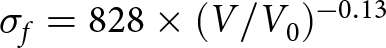 $\sigma_f = 828\times (V/V_0)^{-0.13}$ (V is the sample volume and the reference volume is V0 = 1 m3, with
  $\sigma_f$ expressed in kPa) but the empirical equations derived exhibit dispersion issues similar to those reported by Timco and O’Brien (Reference Timco and O’Brien1994). In addition, in these studies, no micromechanism was identified that would explain this volume effect on the flexural strength of ice.
The main issue is probably the systematic lack of information about the microstructural properties preventing the connection of the flexural strength (usually taken as the mean measured stress to failure) scattering to the distribution of defects in the microstructure. Indeed, brittle-like materials subjected to a quasi-static tensile stress are expected to fail under random stresses due to the development of a single crack triggered by a microstructural defect (Jayatilaka and Trustrum, Reference Jayatilaka and Trustrum1977). As shown by (Hawkes and Mellor, Reference Hawkes and Mellor1972; Schulson and others, Reference Schulson, Lim and Lee1984; Druez and others, Reference Druez, Cloutier and Claveau1987) and reviewed in (Schulson and Duval, Reference Schulson and Duval2009), below −10°C, polycrystalline ice can be mechanically considered a brittle material when loaded in tension at rates above 10−7 s−1 and at rates above 10−4–10−3 s−1 in compression. The triggering defect can be a micro-crack, an inclusion, a pore or an impurity, for instance, and its critical activation stress (equivalent to the failure stress in quasi-static conditions) is supposed to be related to its nature and/or its size. As an illustration, the tensile strength of equiaxed and non-porous ice was found to decrease with increasing grain size, when cracks nucleate at grain boundaries (Currier and Schulson, Reference Currier and Schulson1982).
So far, probability distribution functions have been used to describe the strength of brittle materials. Among them, the Weibull distribution (Weibull, Reference Weibull1951) is state of the art for the mechanical design procedure, although the strength data are not necessarily distributed according to a Weibull statistic law. To our knowledge, few studies applied the Weibull approach on ice material. Tozawa and Taguchi (Reference Tozawa and Taguchi1986); Parsons and Lal (Reference Parsons and Lal1991) and Parsons and others (Reference Parsons1992) described the failure stresses of ice samples with a statistical approach by applying a Weibull or a double exponential distribution to data resulting from various bending experiments. Again, in these works, little is known about the microstructural properties of the ice samples. Parsons and others (Reference Parsons1992) identified an effect of the sample volume on the measured strength that could not be described by the Weibull model. As demonstrated by Danzer and others (Reference Danzer, Supancic, Pascual and Lube2007) and Forquin and others (Reference Forquin, Rota, Charles and Hild2004) for ceramics, the applicability of the Weibull distribution parameters, derived from flexural tests, is limited to volumes representative of the distribution of activated defects from which these parameters were originally determined.
As an alternative to a statistical representation of the defect population, 3D characterizations can be used to evaluate the exact defect distribution, e.g. pores, and identify the active defect population in a given load frame (Forquin and others, Reference Forquin, Blasone, Georges and Dargaud2021).
In the present study, we will consider isotropic ice as the brittle material of interest, within which the defect population is made of pores of various size and density. The main objectives are, first, to evaluate the effect of porosity on the flexural strength of ice, and second, to investigate the underlying failure mechanisms. In particular, we aim to identify the specific pore populations responsible for crack initiation under flexural loading.
To do so, the flexural strength has been measured during two distinct experimental campaigns of three-point bending tests. The ice samples used were grown in the laboratory, in order to control the microstructure and the porosity. The density and distribution of pore sizes have been characterized in 3D by means of X-ray Micro-Computed Tomography ( $\mu$CT) measures, down to a voxel size of 7
  $\mu$m.
The determination of Weibull parameters allowed us to highlight the activation of different defect populations according to the ice microstructure considered. Following our hypothesis regarding the role of pores as critical defects, the relationship between pore size and failure stress is further explored by applying Griffith’s fracture criterion to derive a critical defect density from the 3D pore distributions, as in (Forquin and others, Reference Forquin, Blasone, Georges and Dargaud2021). This critical defect distribution is further used to study the volume effect on the flexural strength of the ice microstructures studied, providing an example and avenue for additional research.
2. Material
2.1. Sample preparation
The samples are made of polycrystalline granular ice grown in the laboratory resulting in microstructures of low porosity (LP) ( $\approx 1--2 \%$) and high porosity (HP) (
 $\approx 7--10 \%$). Both types of microstructure are obtained by a growth technique inspired by Barnes and others (Reference Barnes, Tabor and Walker1971) and described in Georges and others (Reference Georges, Saletti, Montagnat, Forquin and Hagenmuller2021). The samples are grown from isotropic seeds made of crushed ice (with a maximum particle diameter of 2 mm) immersed in water at 0°C. The slurry is placed on a Peltier element (−15°C), in a 0°C cold room whose temperature fluctuates within ± 0.2°C, to grow gently from bottom to top. To obtain the LP microstructure, the crushed ice was pumped for 1 hour using a primary vacuum pump before the water is added. In order to produce the HP microstructure, the air trapped between the crushed ice grains is kept (no pumping). LP samples show no visible porosity and are slightly opaque, whereas large pores are visible in HP samples. After demoulding, the samples are stored for 24 hours at 0°C. This annealing stage enables relaxation of the freezing stresses and homogenization of the grain size by normal grain growth. The length of the cylindrical samples, before machining, is about 20–25 cm. Samples with pores larger than 10 mm were discarded after machining based on a naked-eye inspection. In addition, one HP sample was excluded post-testing after its fracture surface revealed two pores larger than 10 mm.
2.2. 2D characterization
In order to provide a detailed 2D characterization of the microstructures, 10 LP and 10 HP samples, not tested but assumed to be representative of the whole sets, were machined in thin square sections of approximately 50 × 50 mm2 and 0.3 mm thickness. An Automatic Ice Texture Analyzer (AITA) (Wilson and others, Reference Wilson, Russell-Head and Sim2003) was used to measure the orientations of the optical axes (the [0001] c-axis of the hexagonal crystalline cell) in all the thin sections obtained. Data so obtained enable one to access the 2D crystalline structure of the samples, i.e. the crystal size and shape and their crystallographic orientations. The c-axis orientations are measured at a resolution of  $20 \ \mu$m, with about 3° of angular resolution (Wilson and others, Reference Wilson, Russell-Head and Sim2003).
Sections analyzed with the AITA, Fig. 1, show isotropic textures, i.e. a rather equiaxed grain shape and an isotropic distribution of c-axis orientations. This qualitative observation is supported by the eigenvalues of the second-order orientation tensor, which are all close to 0.3, as expected for an isotropic distribution. Grain areas were measured by extracting grain contours with morphological tools from the orientation color-coded images. The grain-size distribution is Gaussian, with average grain sizes of 1.17 mm and 1.28 mm for LP and HP samples, respectively.
Microstructures color-coded with the c-axis orientation for low porosity (LP) (left) and high porosity (HP) (right) samples. Data are obtained with the Automatic Ice Texture Analyzer from thin sections. Rounded black areas correspond to pores in (right).

2.3. 3D characterization
X-ray Micro-Computed Tomography, µCT, is a convenient non-destructive method to evaluate the 3D microstructure of heterogeneous materials and, more specifically, to quantify the size, shape and space distributions of pores. In order to characterize these distributions and their statistical significance, scans with different voxel sizes and geometries were made on several HP and LP samples.
2.3.1. Description of the µCT configuration
Scans were performed with the TomoCold DeskTom130 (RX Solutions) tomograph located in a cold room set at −20°C at the CNRM-CEN (Centre National de Recherche Météorologique - Centres d’Etudes de la Neige), Grenoble. The source is composed of a 150 kV RX tube with a focal size that can reach 5 µm and of a flat panel detector with an active surface of about 1920 × 1536 pixels (physical pixel size of 127 µm). In order to provide a meaningful statistical distribution of pores, including the largest ones, large cylindrical samples of  $\oslash \times h = 45 \times 120$ mm3 were analyzed (later called samples LPT(L) or HPT(L)) with a voxel size of 27 µm. Full scans for LPT(L) and HPT(L) samples are reconstructed from four stacks scanned at different sample heights (by a vertical translation of the source and detector). Smaller volumes of
  $\oslash \times h = 12.7 \times 9.2$ mm3 (samples LPT(S) or HPT(S)) were analyzed to a higher resolution of 7 µm voxel size. For the latter, partial scans were done out of samples of
  $\oslash \times h = 20 \times 40$ mm3. This lower voxel size was necessary to better identify the smallest pore population. Specific settings of the µCT analyses are listed in Table 1.
Settings of the µCT analyses performed with the TomoCold. LP and HP stand for low and high porosity, respectively. (S) and (L) for Small and Large area of analysis. See text for more details.

2.3.2. Image post-processing
For every scan, a 3D image was reconstructed from the acquired radiographs. A ring filter with a 20 voxel kernel was applied in order to remove ring features that are acquisition artifacts. After reconstruction, scans consisted of approximately  $4500 \times 1660 \times 1660$ voxels for large samples and
  $1300 \times 1800 \times 1800$ voxels for small samples, the value of which spreads between 0 (black) and 65536 (white). A contrast enhancement was performed prior to conversion into 8 bit images to obtain reproducible gray level histograms. This operation allowed us to apply the same threshold method for each scan of the same sample type (HP or LP). Typical images (8-bit) scanned with a voxel size of 7 µm and 27 µm are shown in Fig. 2. Figure 3 presents the gray level distributions obtained for the two sample types. Both show similar distributions regardless of the scanning resolution.
2D slices (8 bits) perpendicular to the sample axis from scans (top left) LPT(L)01, (top right) HPT(L)01, (bottom left) LPT(S)01 et (bottom right) HPT(S)02.

Probability density function of voxel grey levels for (Left) LP and (Right) HP samples.

Segmentation, which enables us to separate ice and air into binary images requires us to separate the two gray-level distributions that result from the raw scans. This threshold step is crucial, in order to minimize the segmentation errors that could lead to an over- or under-estimation of the porosity by artificially enlarging or reducing the volume occupied by air (or ice, although it is here the dominant phase), especially for small features that are particularly sensitive to the threshold value.
We assume that both distributions can be approximated by Gaussians, and the threshold value is chosen at the intersection between the two Gaussian fits of each phase (in red and yellow for air and ice, respectively, Fig. 3). Finding an accurate threshold is more subtle for histograms associated with LP samples, since the pore density and size are much smaller. A pseudo-maximum for the air phase is therefore manually determined.
The binary images obtained are treated via SPAM (The Software for the Practical Analysis of Materials) (Stamati and others, Reference Stamati2020), an open-source Python package. During this step, each group of isolated or aggregated black voxels (air) is labeled. Some small labels can be artifacts from Gaussian noise (due to photon scattering during µCT acquisition) and it is preferable to set a minimum label size. Consequently, only labels corresponding to more than 10 voxels,  $\sim 2 \times 10^{-4}$ mm3 (
 $\sim 3.4 \times 10^{-6}$ mm3) for a voxel size of 27 µm (7 µm) were taken into account and considered as pores.
Pores are characterized by their equivalent radius  $r_{eq}$ defined as the radius of a sphere whose volume is equal to the volume of the pore. A coefficient of sphericity
  $\Psi$ is used to characterize the geometry of the pores.
  $r_{eq}$ and
  $\Psi$ are given by:
 \begin{equation}
r_{eq} = \sqrt[3]{\frac{3 V_p}{4 \pi}}
\quad\text{and} \quad
\Psi = \frac{\pi^{1/3} (6V_p)^{2/3}}{A_p}
\end{equation}
\begin{equation}
r_{eq} = \sqrt[3]{\frac{3 V_p}{4 \pi}}
\quad\text{and} \quad
\Psi = \frac{\pi^{1/3} (6V_p)^{2/3}}{A_p}
\end{equation} with  $V_p$ and
  $A_p$ being the volume and the area of the ideal ellipsoid that fits the porosity. The technique described by Ikeda and others (Reference Ikeda, Nakano and Nakashima2000) was applied to estimate the length of the principal axes of this ellipsoid. A coefficient of sphericity close to 1 indicates almost spherical pores, while pores are nearly flat when the coefficient tends to 0. We can also collect the coordinates (
 $x$,
$x$,  $y$,
$y$,  $z$) of the center of mass of each pore in the scanned volume.
2.3.3. Pore size and shape distributions
The number of scans evaluated for both types of microstructure is sufficient to verify that the growth procedure led to reproducible microstructures. Figure 4 represents the mean cumulative distributions of the pore size ( $r_{eq}$) for the LP (in blue) and HP (in red) microstructures. These distributions gather results obtained from scans at 7 and 27 µm. The distribution of pore shapes is shown in Fig. 5. Scans at 7 µm allowed us to identify pores of equivalent radius as low as 0.009 mm. From these distributions, we classified the pores into three different populations. The population L (Large) is characterized by large spherical pores (
 $r_{eq} \gt 0.3$ mm and
  $\Psi$ close to 1) and is observed mainly in HP samples (only 12 pores of this population have been identified in LP samples). Pores whose equivalent radius is between 0.1 and 0.3 mm belong to population M (Medium). The pores belonging to this population have on average a lower sphericity coefficient (
 $0.4 \leq \Psi \leq 1$) than population L, for both types of microstructure. Population S (Small) includes pores whose equivalent radius is less than 0.1 mm.
Mean cumulative distribution of pore size ( $r_{eq}$) for LP (blue) and HP (red) microstructures. Results from scans at 7 microns (dark distributions) and 27 microns are superimposed.

Sphericity coefficient of pores from (left) LP and (right) HP samples. Colored (blue and red) points correspond to the results from one sample of each scanned at 27 microns. Darker and empty circles represent the sphericity coefficient of all pores detected in all samples scanned at 7 microns.

3. Bending tests
3.1. Sample design
From the cylindrical samples grown (see Section 2.1), parallelepipedic samples were milled in a cold room at  $-10^{\circ}\mathrm{C}$. Milling allowed us to ensure that the loaded faces have a parallelism default lower than 0.01%.
Pores are considered here as active defects in these ice microstructures. The distributions of pore size and shape presented in the previous section reveal the existence of different pore populations classified into small (S), medium (M) and large (L) pores. Depending on the sample dimensions and the test configuration, one or even two pore populations may reach sizes sufficient to act as the critical defect and therefore control the flexural strength. Indeed, if the critical defect size lies in the intermodal region of the pore size distribution, failure may be governed jointly by the two populations. Samples must be sized to contain a statistically representative number of pores in the population of interest. HP samples, for example, were oversized to ensure that there were enough large pores (population L) in the volume tested. LP samples containing smaller pores were given a smaller size. The dimensions of the samples were  $L \times h \times b= 140 \times 40 \times 20$ mm
 $^3$ for the HP microstructure (24 samples) and
  $L \times h \times b= 60 \times 20 \times 10$ mm
 $^3$ for the LP microstructure (27 samples). The density distributions of the LP and HP samples considered in this study are illustrated in Fig. 6. Five small HP samples (called HPS) (
 $L \times h \times b= 60 \times 20 \times 10$ mm
 $^3$) were also manufactured to test a volume effect on the flexural strength.
Density of LP ( $\Delta \rho \pm 13$ kg.m−3) and HP (
 $\Delta \rho \pm 5$ kg.m−3) bending samples in their final dimensions.

3.2. Experimental device and procedure
Experiments on HP samples were carried out in the 3SR laboratory (Grenoble, France) during a first campaign. A second experimental campaign, where the LP and HPS samples were tested, was led by using the LaMCoS facilities (Lyon, France). The experimental procedure was kept as similar as possible between campaigns. In both cases, a three-point bending device was mounted in a uniaxial press controlled by displacement rate. The presses were coupled with a climatic chamber supplied with liquid nitrogen to regulate the sample temperature during the tests. The choice of a test temperature of  $-30^{\circ}\mathrm{C}$ was made to limit possible plastic deformations during experiments (Schulson and Duval, Reference Schulson and Duval2009).
Some differences in the loading configuration existed between the two campaigns. At 3SR, the span between the lower supports was 120 mm, and all supports had a curvature radius of 7 mm. At LaMCoS, the span was 50 mm, with the lower supports having a curvature radius of 2.5 mm and the upper support a radius of 5 mm.
Before loading, the samples were stored in a freezer ( $-30^{\circ}\mathrm{C}$) located near the climatic chamber to reduce the time of exposition to ambient temperature (
 $20^{\circ}\mathrm{C}$) during sample transfer to a few seconds. Markers were used to facilitate the setting of the ice samples and also to ensure an optimal position with respect to the loading device. After several openings and closings of the climatic chamber, frost began to develop on the loading supports. The supports were systematically brushed immediately before each test, although the procedure had to be performed very quickly, so it is possible that small ice particles occasionally remained. Such residual frost could introduce a slight contact compliance between the sample and the supports. After failure, fragments of the tested samples were carefully kept for observations in the cold room.
During the second experimental campaign (LaMCoS), we used a high-speed camera (Phantom V710 camera, 80 000 fps) placed in front of the climatic chamber (see Fig. 7) to study the failure kinetics and to locate the fracture plane.
Left: High-speed camera pointing toward the climatic enclosure (LaMCoS). Right: Three-point bending devices.

3.2.1. Loading rate
The ductile-to-brittle transition of polycrystalline ice under tensile loading depends on the strain rate and occurs at approximately 10−7 s−1 at −10°C (Schulson, Reference Schulson2001). The results of the bending tests are analyzed in the framework of the linear elastic theory of beams, which assumes an elasto-brittle behavior of the ice samples. The displacement rate was set at  $\delta = 4 \times 10^{-6}$ m.s−1 for the 3SR campaign. Regarding the dimensions of HP samples and according to the linear elastic theory for three-point bending, the resulting strain-rate can be estimated by:
 \begin{equation}
{\varepsilon} = \frac{6h \delta}{L'^2}=2.7 \times 10^{-5} s^{-1}
\end{equation}
\begin{equation}
{\varepsilon} = \frac{6h \delta}{L'^2}=2.7 \times 10^{-5} s^{-1}
\end{equation} with  $L' = 120$ mm the distance between the bottom supports and h the height of the sample. The applied strain rate is almost two orders of magnitudes faster than the expected ductile to brittle transition at −10°C, although it will be shown in Section 3.3 that the loading path of several samples does not show a perfectly linear behavior. Therefore, during the second campaign in LaMCoS, the displacement rate was increased to
  $\delta = 5 \times 10^{-5}$ m.s−1, i.e.
  $\Dot{\varepsilon} = 2.4 \times 10^{-3}$ s−1 according to equation 2. Previous research (Timco and O’Brien, Reference Timco and O’Brien1994; Petrovic, Reference Petrovic2003; Timco and Weeks, Reference Timco and Weeks2010) has established that the flexural strength of ice does not depend on the strain rate as long as the loading is purely elastic. The difference in strain rate between both campaigns is thus expected to have a negligible effect except if plasticity does indeed come into play.
The flexural strength  $\sigma_f$ is obtained from the maximum force
  $F_{max}$ measured just before failure by:
 \begin{equation}
\sigma_f = \frac{3 F_{max} L'}{2bh^2}
\end{equation}
\begin{equation}
\sigma_f = \frac{3 F_{max} L'}{2bh^2}
\end{equation} with  $b$ the width of the sample.
3.3. Results
3.3.1. Loading curves
The loading curves measured during the two experimental campaigns are presented in Fig. 8. The times to failure measured during the 3SR campaign have a large variability, from 20 to 110 s. The load drops are sharp and sudden, as expected during a purely brittle failure. However, for tests with a failure time exceeding 70 s, the loading path is not linear. This phenomenon could be related to contact problems, but also to the activation of some plasticity, at least locally, in particular for the experiments performed at a strain rate of 2.7 $\times$10−5 s−1. Local maxima (slight load drops) are also visible on the loading curve of sample HP20. The most likely explanation is the breaking or motion of frost particles on the bottom and/or upper supports.
Loading curves from the campaign in (top) LaMCoS and in (bottom) 3SR. Black dashed curves (top) show the HPS samples tested during the campaign in LaMCoS.

During the LaMCoS campaign, performed at a higher loading rate (2.4 $\times$10−3 s−1), time to failure occurred in a narrower range, between 15 and 20 s (except for samples LP02 and LP07). As for the 3SR campaign, the load drop is sudden and sharp, as expected during a purely brittle failure.
3.3.2. Observations of fracture patterns
As an illustration of a classical test behavior, images taken from the high-speed camera at different critical times of failure for the LP04 and HPS03 samples are shown in Fig. 9 and Fig. 10 respectively. The fracture planes appear to be the result of the propagation of a single crack triggered in the lower part of the sample, which is subjected to a tensile stress. The time for the crack to propagate throughout the sample, as observed in the images, is about 30 to 40 µs, which is very close to the estimated value for crack propagation in ice (35 µs with a crack propagation velocity of  $k\times C_0$, with
  $C_0 = 3000$ m s−1, the sound wave velocity in LP ice (Georges and others, Reference Georges, Saletti, Montagnat, Forquin and Hagenmuller2021) and
  $k=0.38$ (Broek, Reference Broek1982)). Narrow microcracks can also be observed just below the upper contact area. These microcracks appear to be local enough not to disturb the tensile stress field in the bottom part, where the main crack is activated. None of these microcracks was observed in the postmortem samples and therefore most likely healed between the test and the analysis in the cold room. We expect similar microcracking to have occurred in the HP samples during the first campaign.
Key moments of the LP04 sample failure (images from the high-speed camera Phantom). The loading axis is symbolized by the white arrow on the upper support. Sample height: 20 mm.

Key moments of the HPS03 sample failure (images from the high-speed camera Phantom). The loading axis is symbolized by the white arrow on the upper support. Sample height: 20 mm.

The fracture surfaces observed in the postmortem samples show low roughness and cracks seem to have propagated without a noticeable shift in direction, indicating that neither other microstructure defects (most likely pores in our case) nor plasticity interfered with crack propagation. We observed two main configurations: (i) a crack starts along the loading direction (that is, where the maximum tensile stress is reached), and propagates straight and vertically, (ii) a crack is triggered on the side (Fig. 11) and the propagation occurs at an angle  $\theta$ with respect to the loading direction and eventually reaches the upper support. This second type of fracturing mode was more commonly encountered in HP samples.
Photos of (top) LP08 and (bottom) LP02 post-mortem samples.

3.3.3. Failure stresses
The forces measured at failure are listed in Table 2 for both experimental campaigns. The flexural strength is calculated using equation 3. The mean flexural strengths are  $\sigma_w(HP) = 1.76 \pm 0.42$ MPa for HP samples (HPS samples excluded) and
  $\sigma_w(LP) = 3.96 \pm 0.37$ MPa for LP samples. An average value of
  $\sigma_w(HPS) = 2.54$ MPa is also measured from the few HPS samples tested under conditions similar to the LP samples. LP samples show significantly higher flexural strengths than HP samples, regardless of the experimental conditions considered for the latter. Large HP samples (tested at 3SR) show a lower average strength than small HP samples (HPS) (tested at LaMCoS).
Bending tests results, with  $T_f$: Time to failure,
  $F_{max}$: Maximum force to failure,
  $\sigma_F$: maximum stress to failure.

4. Discussion
4.1. The ice flexural behavior
In-depth characterization of the studied microstructures ensures a high level of confidence in the reproducibility of the samples. In addition, the experimental conditions—temperature and mechanical loading—were repeatable. When available, image analysis and fracture surface observations in post-mortem samples revealed no evidence contradicting the use of linear beam elasticity theory to determine ultimate failure stress. Only a few highly porous (HP) tests may involve plastic deformation despite the imposed loading rate.
To the best of our knowledge, no experimental data set on the flexural behavior of ice in the literature offers the same degree of control. These results provide the scientific community with a rigorously documented and robust dataset on the flexural response of isotropic ice with controlled microstructures.
The flexural strengths measured for the LP and HP ices are consistent with existing results (Timco and Frederking, Reference Timco and Frederking1983; Aly and others, Reference Aly, Taylor, Bailey Dudley and Turnbull2019). Using the empirical equation  $\sigma_f = 828V^{-0.13}$ from Aly and others (Reference Aly, Taylor, Bailey Dudley and Turnbull2019) with
  $V$(LP)
 $ = 1.2 \times 10^{-5} \mathrm{m}^3$ and
  $V$(HP)
 $ = 1.12 \times 10^{-4} \mathrm{m}^3$, the estimated strengths are
  $\sigma_f$(LP) = 3.6 MPa and
  $\sigma_f$(HP) = 2.7 MPa. However, it is important to emphasize that relevant comparisons with previous data are only meaningful when microstructure, sample geometry and loading conditions are similar. This is not the case here, as most existing studies focus on natural ice or artificial freshwater/atmospheric ice, often with very different experimental setups.
As expected, a volume effect exists between samples of different dimensions, with flexural strength increasing as volume decreases. However, the volume effect observed between HP and HPS samples should be interpreted with caution, as statistical robustness is limited due to the small number of HPS tests (only five). This trend has been repeatedly observed in ice (Timco and O’Brien, Reference Timco and O’Brien1994; Aly and others, Reference Aly, Taylor, Bailey Dudley and Turnbull2019), and other brittle materials such as concrete or glass (Nguyen and others, Reference Nguyen, Kim, Ryu and Koh2013; Wang and others, Reference Wang, Fu and Manes2021). In our study, both microstructures exhibit similar properties except for porosity, the primary difference being the presence of pore population L in HP samples. As a result, the observed volume effect is closely related to the characteristics of the porosity distribution.
There are still limited data in the literature to support meaningful comparisons regarding the influence of porosity on the mechanical response of ice. In (Kermani and others, Reference Kermani, Farzaneh and Gagnon2008), laboratory-made atmospheric ice with a porosity of approximately 8.5 $\%$ exhibited a lower flexural strength (2 MPa) than samples with a lower porosity of 2.9
 $\%$ (2.8 MPa). The samples, with dimensions
  $L \times h \times b = 70 \times 20 \times 40$ mm3, were tested at a strain rate of approximately
  $2 \times 10^{-3}$ s−1 and at a temperature of −20°C. The authors attributed the reduction in strength to a high density of pre-existing cracks in the more porous samples. In contrast, Gagnon and Gammon (Reference Gagnon and Gammon1995) reported the opposite trend: the flexural strength of iceberg and glacier ice increased with porosity and pore density. They proposed that intragranular pores could soften the grains, thus reducing crack-initiating stresses at grain boundaries.
Here, images from the camera and the study of fracture surfaces did not allow direct conclusions about the role of porosity. Based on the hypothesis that pores act as active defects within the microstructure, it can be expected (as mentioned by Jayatilaka and Trustrum (Reference Jayatilaka and Trustrum1977); Danzer and others (Reference Danzer, Supancic, Pascual and Lube2007) or Forquin and others (Reference Forquin, Rota, Charles and Hild2004) for other brittle materials) that the activation stress of these defects is related to their size. This hypothesis could also explain the observed differences in flexural strengths between HP and HPS samples, as it is statistically more likely to find larger pores in larger samples. In the following sections, we will further explore this hypothesis and attempt to validate it by trying to identify the population of pores responsible for sample failure.
4.2. Characterization of the defect population with the Weibull model
As is commonly done in the literature to characterize the strength variability and assess the probability of failure in brittle materials (Parsons and Lal, Reference Parsons and Lal1991; Steen, Reference Steen1999; Boyce and others, Reference Boyce, Grazier, Buchheit and Shaw2007; Li and others, Reference Li, Guan, Yuan, Yin and Li2021), we apply the Weibull statistical model to our dataset. The Weibull model enables the association of a failure probability distribution with a critical stress of solicitation, assuming that activated defects in the material follow a Weibull distribution. In the following, we check the applicability of the Weibull model to our bending test results and its ability to identify the population of pores responsible for sample failure.
4.2.1. The Weibull distribution
Quasi-brittle or brittle materials subjected to a quasi-static tensile loading fail at random stresses. For a given applied stress, the failure occurs with a probability  $P_f$. This probability is related to the stress field within the sample and to the properties of the defect distribution (nature, size, density, orientation, etc.) in the sample volume
  $V$. In the following, and on the basis of the experimental results, the hypothesis is made that pores are the active defects in the ice samples studied.
The failure statistic model suggested by Weibull (Reference Weibull1951) is based on the hypothesis of the weakest link. In other words, the failure of the weakest element in a volume, once its critical stress of activation is reached, induces the ruin of the whole structure. This assumption is valid, provided that the interaction between defects during failure can be neglected. From (Weibull, Reference Weibull1951), the failure probability Pf of a volume V for a given principal positive stress  $\sigma$ supposed to be uniformly distributed in the volume is:
 \begin{equation}
P_f = 1 - exp(-\lambda_t V)
\end{equation}
\begin{equation}
P_f = 1 - exp(-\lambda_t V)
\end{equation} where  $\lambda_t$ represents the density of critical defects.
In the three-parameter-based Weibull distribution, this density is linked to the maximum positive principal stress by:
 \begin{equation}
\lambda_t = \lambda_0 \left(\frac{\sigma - \sigma_u}{\sigma_0} \right)^m
\end{equation}
\begin{equation}
\lambda_t = \lambda_0 \left(\frac{\sigma - \sigma_u}{\sigma_0} \right)^m
\end{equation} where  $\lambda_0 \sigma_0^{-m}$ is the so-called Weibull scale parameter.
  $\sigma_u$ is the threshold stress under which the material does not fail.
A two-parameter distribution (that is,  $\sigma_u = 0$) often shows a good representation of the scattering of failure stresses, as observed by Danzer and others (Reference Danzer, Supancic, Pascual and Lube2007) for ceramics and more specifically by Parsons and others (Reference Parsons1992) for polycrystalline ice. As a consequence, the failure probability can be expressed as follows:
 \begin{equation}
P_f = 1-exp(-\lambda_0 V (\frac{\sigma}{\sigma_0})^m)
\end{equation}
\begin{equation}
P_f = 1-exp(-\lambda_0 V (\frac{\sigma}{\sigma_0})^m)
\end{equation} where the scale parameter ( $\lambda_0 \sigma_0^{-m}$) and the Weibull modulus (m) are the two parameters that describe the Weibull distribution.
The Weibull modulus is a dimensionless parameter representing the failure stress scattering. Materials with a high value of m tend to show a deterministic behavior, while materials with a low value of m will present a more scattered failure stress distribution. The mean failure stress is used to deduce the scale parameter by:
 \begin{equation}
\sigma_w = \sigma_u + \sigma_0 (V \lambda_0 )^{-1/m} \Gamma \left( \frac{m+1}{m} \right)
\end{equation}
\begin{equation}
\sigma_w = \sigma_u + \sigma_0 (V \lambda_0 )^{-1/m} \Gamma \left( \frac{m+1}{m} \right)
\end{equation} with  $\Gamma$ the gamma function, also known as the Euler integral of the second kind.
The corresponding standard deviation ( $\sigma_{sd}$) is expressed as:
 \begin{equation}
\sigma_{sd}^2 = \sigma_0^2 (V \lambda_0 )^{-2/m} \Gamma \left( \frac{m+2}{m} \right) - (\sigma_w - \sigma_u )^2
\end{equation}
\begin{equation}
\sigma_{sd}^2 = \sigma_0^2 (V \lambda_0 )^{-2/m} \Gamma \left( \frac{m+2}{m} \right) - (\sigma_w - \sigma_u )^2
\end{equation} As explained in (Forquin and Hild, Reference Forquin and Hild2010), the ratio between the standard deviation and the mean failure stress is a continuously decreasing function of m bounded by the functions  $1/m$ and
  $\pi / \sqrt{6} m \approx 1.29/m$.
The Weibull approach is classically used to characterize the defect population when a sample of a given volume V is subjected to a stress field up to failure. When this stress field is heterogeneous, such as during a bending test, an effective volume Veff is considered instead of the volume V of the sample. The effective volume corresponds to the volume loaded by a uniform stress field for which the same level of maximum stress leads to the same failure probability as within V (Davies, Reference Davies1973). The effective volume thus depends on the heterogeneity of the stress field near the positive maximum stress and on the distribution of critical defects in the sample. From Davies (Reference Davies1973), for the three-point bending tests, the effective volume can be approximated by:
 \begin{equation}
V_{eff} = \frac{V}{2(m+1)^2}
\end{equation}
\begin{equation}
V_{eff} = \frac{V}{2(m+1)^2}
\end{equation}4.2.2. Determination of the Weibull parameters
The least squares method is probably the most commonly used to determine the Weibull modulus from experimental tensile failure stresses. Other methods exist, such as the method of moments or of the maximum likelihood estimation, and have been applied in Parsons and Lal (Reference Parsons and Lal1991) on ice.
The first step consists of estimating an empirical cumulative distribution of the probability of failure from the results of the bending or tensile tests. To do so, experimental failure stresses are sorted in an ascending manner. For every failure stress, a rank i (integer) is assigned that corresponds to its position in the ranking. The empirical failure probability is then computed as
 \begin{equation}
P_f = \frac{i-0.5}{N}
\end{equation}
\begin{equation}
P_f = \frac{i-0.5}{N}
\end{equation} where  $N$ is the number of mechanical tests carried out.
Afterward, it is possible to build the so-called Weibull diagram, where the inverse logarithm of survival probability ( $P_s = 1-P_f$) is a function of the applied stress. From the previous equations, it is expressed as follows:
 \begin{equation}
ln(-ln(1-P_f)) = m ln(\sigma_m) + ln(V_{eff} \frac{\lambda_0}{\sigma_0^m})
\end{equation}
\begin{equation}
ln(-ln(1-P_f)) = m ln(\sigma_m) + ln(V_{eff} \frac{\lambda_0}{\sigma_0^m})
\end{equation} This equation implies that, when the strength scattering of the material follows a Weibull distribution, the data can be fitted by a linear function whose slope is the Weibull modulus. The scale parameter  $\lambda_0 \sigma_0^{-m}$ is obtained from equation 7 once the mean failure stress is known.
4.2.3. Weibull parameters for LP and HP ice samples
The failure probability expressed in equation 10 was obtained from the data of the bending tests carried out on LP and HP ice samples. The cumulative distributions of failure probability plotted in Fig. 13 give access to the corresponding Weibull parameters (Table 3).
Cumulative distributions of experimental failure probability as a function of HP (red markers) and LP (blue markers) samples failure stress. The black dotted lines represent the predictions of the Weibull model given by the equation 6, obtained by the least square method.

Weibull parameters of LP and HP microstructures, with  $m$ the Weibull modulus,
  $\lambda_0 \sigma_0^{-m}$ the scale parameter,
  $V_{eff}$ the effective volume,
  $\sigma_w$ the mean stress to failure,
  $\sigma_{sd}$ the standard deviation and
  $\alpha$ the linear regression coefficient in Weibull’s diagram.

Please note that HPS samples (from the LaMCoS campaign) are not considered here since too few tests were performed to secure a robust statistical analysis. Keeping in mind the hypotheses behind the Weibull model, the determination of the modulus  $m$ was made after taking the following precaution. Samples LP26 and LP27 show a higher failure stress than all other LP samples. The failure of these samples may be due to the activation of a pore from a population of a characteristic size smaller than that of all other LP samples. By removing these data (from samples LP26 and LP27) that are outside the trend to calculate the Weibull parameters, we are more likely to characterize a specific defect population common to most of the samples studied, under the frame of the Weibull model. In doing so, the resulting mean failure stress differs slightly from the one calculated in Section 3.3 (see Table 3).
Both HP and LP samples show a failure stress probability that can be reasonably fitted by a linear curve in the Weibull diagram (log-log scale), which confirms the unimodal nature of the activated defect distribution. With  $m_{LP} \gt \gt m_{HP}$, the Weibull parameters reveal a more deterministic behavior of the LP samples than of the HP samples, which is consistent with a lower dispersion in the failure stresses of the LP samples. The difference in the estimated Weibull parameters between the two types of samples reveals that their failure is the result of two different populations of activated defects. A higher Weibull modulus also indicates that the sizes of the activated defects are distributed over a narrower distribution. The corresponding effective volume
  $V_{eff}$ is much smaller than the actual sample volume, almost 500 times smaller for LP samples and 100 times smaller for HP samples.
From these analyses, we can hypothesize that the critical defects in the LP - respectively HP - samples are very likely coming from the population of medium pores (population M) - respectively large pores (population L). If the population of small pores (population S) had played a role for both microstructures, the Weibull diagrams (Fig. 12) would have been much more similar. As mentioned in Section 3, some plasticity may have come into play during the tests on the HP samples. Plasticity is expected to increase the failure stress, resulting in a slight overestimation of the Weibull modulus. We expect this overestimation to be low enough not to contradict the present analysis.
Calibration of the shape parameter  $Y$. (Left) microstructure LP and (right) microstructure HP. The yellow distributions correspond to the shape parameter chosen. The boundaries indicating the S, M and L populations are valid only for
  $Y = 1.1$ (LP) and
  $Y=0.8$ (HP).

The primary conclusion of this Weibull analysis is that failure results from the activation of two distinct defect populations for the two types of samples studied. The role of the microstructure in the failure mechanisms, the porosity here, is therefore clearly identified. To assess whether populations M and/or L contribute to sample failure, we need to advance our analysis by converting, with the appropriate failure criterion, the pore size distribution into a critical defect distribution function based on the applied stress.
4.3. Explicit estimation of the critical defect distribution from µCT measurements
In the following, we will work within the framework of linear elastic fracture mechanics and use the Griffith/Irwin failure criterion as done by Trustrum and Jayatilaka (Reference Trustrum and Jayatilaka1983); Forquin and others (Reference Forquin, Rota, Charles and Hild2004) and Danzer and others (Reference Danzer, Supancic, Pascual and Lube2007). The Griffith criterion considers that a crack of length  $2a$ is unstable when the stress intensity factor
  $K_I$ near the crack tip exceeds the fracture toughness
  $K_{Ic}$. This statement reads:
 \begin{equation}
\sigma_c = \frac{K_{Ic}}{Y \sqrt{\pi a}}
\end{equation}
\begin{equation}
\sigma_c = \frac{K_{Ic}}{Y \sqrt{\pi a}}
\end{equation} where  $Y$ is a theoretical shape parameter related to the geometry of the crack. It is bounded by two values
  $Y = 1$ and
  $Y=2/\pi$, which correspond to theoretical situations (Sack, Reference Sack1946). The fracture toughness
  $K_{Ic}$ of ice has not been measured in this work, but can be estimated from the literature. Fracture toughness values obtained from natural ice samples have been excluded due to the frequent lack of knowledge or control over the microstructure and impurity content in the samples, which can differ significantly from the laboratory ice studied here. Nixon and Schulson (Reference Nixon and Schulson1988) evaluated the fracture toughness from laboratory-made polycrystalline ice samples, with microstructures similar to those of our LP samples. They measured the variation of
  $K_{Ic}$ with grain size and obtained values between 67 and 137 kPa m
 $^{0.5}$ for grain sizes ranging between 1.6 and 9.3 mm in diameter. The grain diameter in our samples being within 1 to 2 mm, the closest value would be that obtained by Nixon and Schulson (Reference Nixon and Schulson1988) with 1.6 mm diameter grain size, that is,
  $K_{Ic} = 91.3$ kPa.m
 $^{0.5}$. In brittle materials,
  $K_{Ic}$ is expected to depend slightly on porosity. The only study we found that tested the impact of porosity on the fracture toughness of ice (Smith and others, Reference Smith, Schulson and Schulson1990) reveals a wide scattering of the data. We will therefore neglect this effect on a first approximation and keep the same value of
  $K_{Ic}$ for both LP and HP samples.
Based on the pore distribution measured by  $\mu$CT, we can now relate a theoretical failure stress to the defect density with equation 12. The shape parameter
  $Y$ remains the only unknown of this approach. Since the real shape of pores in the samples is likely to be very different from the ideal crack shapes considered in the Griffith model, it is illusory to try to determine a value from observations.
In Fig. 13, the relationship between the defect density and the critical failure stress is plotted for three values of  $Y$. The defect density derived from the Weibull parameters (see equation 5), and therefore based on failure stress measured during our bending tests, is superimposed on these plots. By default,
  $Y$ is selected so that the defect density matches the Weibull defect distribution at the experimental mean failure stress
  $\sigma_w$. By doing so, it is important to emphasize that the parameter
  $Y$ partially compensates, if needed, for the value of the fracture toughness adopted in our study. The parameter
  $Y$ thus obtained is
  $1.1$ for LP samples and
  $0.8$ for HP samples. Both values are very close to the ones found by Forquin and others (Reference Forquin, Blasone, Georges and Dargaud2021) for a SiC ceramic and Ultra-High Performance Concrete (UHPC).
The best match between the Weibull predictions and the defect density distribution estimated from measured pore-size distributions occurs in the M population range for LP samples and in the L population range for HP samples.
The range of defect density is further narrowed by selecting only the data bounded by the minimum and maximum failure stresses measured during the bending experiments. These ranges are [3.26–4.30 MPa] and [1.11–2.35 MPa] for LP and HP samples, respectively. In these ranges, the defect density follows a power-law relation with the critical failure stress, represented in Fig. 14. Under the hypotheses of the Weibull model, the power-law relation can be interpreted as a Weibull diagram and a Weibull modulus can be extracted and compared to the value measured in Section 4.2. The excellent match obtained for LP samples demonstrates that, if our hypotheses are valid, the pores of the M population indeed acted as critical defects in the initiation of failure for this microstructure.
However, for the HP microstructure, the match is not very good with the Weibull distribution. We suggest that this mismatch is due to the heterogeneity in pore size in population L. Indeed, with larger pores, the hypothesis of the sample being a representative elementary volume is more questionable. The effective volume calculated from the Weibull model is 1.22 cm $^3$ (Table 3). For such a volume, the probability of encountering pores with an equivalent radius greater than 2 mm is less than 10%. Larger samples or, at least, a larger number of tests could have been necessary to provide robust enough statistics to recover representative Weibull parameters of the population L of pores.
Focus on the defect density distribution measured by  $\mu$CT as a function of the critical failure stress, in the range of the measured failure stress during experiments on HP (red) samples and LP (blue) samples. The black lines represent the fit of Weibull diagrams from Figure 12 and the red and blue dot lines represent an equivalent Weibull modulus obtained directly from the data.

Beyond the interpretation regarding the role of pores in the failure mechanisms, this analysis demonstrates that it is possible to consider the actual distribution of defects, in this case, pores, to predict the flexural strength of ice, provided an appropriate failure criterion and representative elementary volumes are used. The advantage of this method is that it can account for the multi-modal nature of the defects present, unlike the Weibull model.
Several key points must be emphasized. First, this method relies on the calibration of the shape parameter  $Y$. By default, we applied the same shape parameter for all pore populations, which may not necessarily correspond to the reality. Then, since the Weibull parameters are used to identify the pore population at play, it is therefore also based on the underlying assumptions behind the Weibull model: failure is purely brittle and due to the activation of the weakest link within the considered volume, neglecting the contribution of any other defect.
4.4. Volume effect
As mentioned above, a volume effect is commonly observed when studying the ice flexural behavior. So far, statistical approaches (Tozawa and Taguchi, Reference Tozawa and Taguchi1986; Parsons and Lal, Reference Parsons and Lal1991; Parsons and others, Reference Parsons1992) have not provided satisfactory results and no underlying micromechanical mechanisms have been proposed. In this context, our aim is to explore whether the method based on the 3D characterization of defect populations, combined with the Griffith criterion, can offer a plausible interpretation for the influence of the volume size on failure stress.
4.4.1. Method of analysis
µCT analyses performed on our ice samples provide large volumes within which pores are located (in the limit of accuracy of the µCT apparatus). In the following, large volumes will be called ‘initial volumes’. Thanks to the SPAM software (see Section 2.3), we are able to extract the exact coordinates ( $x$,
$x$,  $y$ and
  $z$) of the mass center for each resolved pore (down to a pore size of 3.43
 $\times 10^{-6}$ mm3 and 1.9
 $\times10^{-4}$ mm3 for scans at 7 µm and 27 µm, respectively).
To evaluate the volume effect described above, the initial volume is discretized into non-overlapping sub-volumes of cubic dimensions. These dimensions vary between roughly 2 and 3800 mm $^3$ according to the properties of the initial volume, meaning its dimensions, the resolution at which it was analyzed and the type of microstructure (LP or HP), see Table 4, to ensure the presence of a minimum of 30 pores in each sub-volume. Three initial volumes scanned at 27 µm are available for each LP and HP microstructure, and three initial volumes scanned at 7 µm for the LP microstructure, but only two for the HP microstructure. In order to remain statistically relevant, we needed to test a sufficiently high number of sub-volumes. A total of 24 sub-volumes are selected in each microstructure, and for each resolution. This number is close to the number of bending tests (25) conducted for each type of microstructure.
Parameters of the sub-volumes tested.  $V_{tot}$ is the size of the initial volumes available. The number of sub-volumes indicates the number of draws in the initial volumes for a given sub-volume size. The number of different sub-volume sizes considered as well as the size range of these sub-volumes are also given.

For each sub-volume, a failure stress was estimated from the Griffith criterion with the assumption that the largest pore is responsible for failure. See Fig. 15 for a schematic representation of the procedure. From a mechanical perspective, the sub-volumes can be considered as effective volumes, assuming that pore activation is induced by a homogeneous tensile stress field within these sub-volumes.
Sketch of the method used to estimate the failure strength on sub-volumes extracted from the exact microstructures. This sketch takes as an example only two different sizes of sub-volumes.

4.4.2. Influence of the sample volume on the failure stress
The evolution of the predicted mean failure stress as a function of the sub-volume size considered is plotted in Fig. 16 for both types of microstructure (LP and HP). Owing to the presence of pores of different sizes (coming from the different pore populations), sub-volumes of the same size present various failure stress predictions resulting in a dispersion around the average value. On these graphs is also represented the prediction of the Weibull model (slope equal to  $-1/m$ in log-log plot) as parameterized in Section 4.2. The error bar associated with this prediction is the one corresponding to the standard deviation provided by equation 8. Furthermore, the volume effect on the flexural strength of freshwater ice as expressed by the equation
  $\sigma_f = 828(V/V_0)^{-0.13}$ in (Aly and others, Reference Aly, Taylor, Bailey Dudley and Turnbull2019) is shown with
  $V = V_{eff} \times 2(m+1)^2$ and
  $V_0 = 1 \mathrm{m}^3$ (
 $\sigma_f$ and 828 are expressed in kPa.).
Evolution of the mean failure stress and the associated standard deviation with the size of the sub-volumes (left) LP and (right) HP microstructures. The mean equivalent radius of the pores activated within a given volume is represented by red diamond symbols. Results are compared with the predictions of the Weibull model and with the equation  $\sigma_f = 828(V/V_0)^{-0.13}$ (
 $\sigma_f$ and 828 are expressed in kPa.) from Aly and others (Reference Aly, Taylor, Bailey Dudley and Turnbull2019).

We observe a good continuity between the prediction resulting from the initial volumes scanned at 27 µm and the ones scanned at 7 µm. For both types of microstructure, the predicted failure stress tends to increase when the sub-volume size decreases. This is consistent with the assumption that the smaller pores become the active defects. Nevertheless, a wider dispersion is predicted for smaller volumes, which reveals that more of those sub-volumes could have been necessary to achieve a better statistic.
The Weibull model offers a relatively good prediction for the HP microstructure (Fig. 16), which is a bit counterintuitive with respect to the results of Section 4.3. An explanation can be found in Fig. 13: if the Weibull distribution does not precisely represent the pores from population L, it does capture the overall trend for populations L and M put together, and it completely diverges for population S. As a result, failure stress is strongly underestimated for the smallest volumes considered when population S likely comes into play (see Fig. 17).
Relative proportion of the pore populations activated as a function of sub-element size in numerical simulations of tensile tests for (Left) LP and (Right) HP microstructures.

The predicted response of the LP microstructure (Fig. 16) is not as well reproduced by the Weibull model that slightly underestimates the response for the small sub-volumes but departs even more from the predicted response for the larger sub-volumes. The only good predictions of the Weibull model are obtained for the sub-volumes whose responses are close to the failure stress experimentally measured. The main defects activated in the LP microstructure are from pore population M in all sub-volumes (Fig. 17), and this population is supposed to be relatively well characterized by the Weibull parameters obtained from bending experiments (cf Section 4.3). This divergence can be explained by the fact that, as shown in Fig. 13, the Weibull distribution is not relevant for the full range of pore size of population M. The largest pores of this population are not well accounted for by the Weibull approximation. These results particularly highlight how challenging it is to predict the effect of volume on the flexural strength of ice using only one set of Weibull parameters. These parameters are specific to the defect population that was activated during the bending tests. When a different defect population becomes predominantly activated, which is statistically more likely as the sample volume changes, the mechanical response of ice is no longer represented by the predictions of the Weibull model.
Similarly, empirical approaches such as those proposed by Timco and O’Brien (Reference Timco and O’Brien1994) and Aly and others (Reference Aly, Taylor, Bailey Dudley and Turnbull2019) can provide a first-order estimate of the volume effect. However, they do not capture the underlying failure mechanisms, and the precision of their predictions may vary significantly with the microstructure of the ice and the volume of the tested sample. As shown in Fig. 16, the prediction from Aly and others (Reference Aly, Taylor, Bailey Dudley and Turnbull2019) differs strongly from the  $\mu$CT-based and the Weibull model predictions for the LP microstructure, while a closer agreement is observed for the HP microstructure.
Finally, it should be noted that the main limitation of our analysis based on the use of the actual defect distribution is related to the  $\mu$CT scan resolution used for porosity characterization. With a finer scan resolution, provided that the micro-mechanisms put forward in our study to explain the flexural behavior of ice are confirmed, it would be possible to predict the stresses at failure of specimens where the pore population S is predominantly activated. This could be the case in configurations where the effective volume decreases or for very high loading rates (Forquin and others, Reference Forquin, Blasone, Georges and Dargaud2021). In contrast, it can be observed that the mean equivalent radius of activated pores never reaches a plateau, even for the largest sub-volumes (red markers in Fig. 16), especially for HP microstructure. This result indicates that the condition of a representative elementary volume (REV) is never met for the population of pores L. Once again, this highlights that the predictive capabilities for the mechanical response of ice are limited by the acquisition settings of the
  $\mu$CT scans.
Despite these limitations, the present analysis was carried out as far as the available data allowed. The combined use of the weakest link hypothesis and a pore-size-dependent critical stress, formulated through the Griffith failure criterion, offers a mechanistic explanation for the volume effect observed in the flexural behavior of ice. This volume effect can indeed be related to the multi-modal nature of the porosity, as the pore population that is preferentially activated explicitly depends on the effective volume considered.
To confirm the validity of this approach, a dedicated experimental campaign should be carried out in the future. The aim of this campaign would be to study the influence of sample volume on the flexural strength of LP and HP ices. The experimental results could then be directly compared with the present numerical predictions, using a wider range of  $\mu$CT scanned sample volumes.
This approach could be extended to the study of natural ice, as the same mechanisms responsible for the volume effect may also be at play. Given the coexistence of various types of defects in natural ice (such as micro-cracks, pores, impurities and brine pockets), it is likely that multiple defect populations compete within a given effective volume, which may complicate the interpretation of experimental results. Moreover, the Griffith failure criterion may not be appropriate for certain types of defects.
5. Concluding remarks
First, the present work provides some of the few robust and reproducible data of flexural strength in isotropic polycrystalline ice with a well-constrained microstructure. The measured failure stresses are in the range 1.1 to 4.9 MPa which is consistent with those reported in the literature (Timco and O’Brien, Reference Timco and O’Brien1994; Aly and others, Reference Aly, Taylor, Bailey Dudley and Turnbull2019). These values depend mainly on two parameters, porosity and sample size. Samples studied have been purposely spread into two families (by construction), a low porosity (LP) microstructure ( $\sim$ 1–2%) and high porosity (HP) microstructure (
 $\sim$ 7–10%). The sample dimensions were
  $L \times h \times b = 60 \times 20 \times 10$ mm and
  $L \times h \times b = 140 \times 40 \times 20$ mm for the LP and HP microstructures, respectively.
Both types of microstructures have been studied by means of X-ray micro-computed tomography ( $\mu$CT) that revealed coexistence of three populations of pores in the samples, namely a small (
 $r_{eq} \lt 0.1~\mathrm{mm}$), a medium (
 $0.1~\mathrm{mm} \lt r_{eq} \lt 0.3~\mathrm{mm}$) and a large (
 $r_{eq} \gt 0.3~\mathrm{mm}$) population. LP samples contained only small- and medium-size pore populations, while HP samples contained all of them.
The lowest strength values are found for the HP microstructure with  $\sigma_w = 1.76 \pm 0.42$ MPa while for the LP microstructure, strengths are nearly twice as high with
  $\sigma_w = 3.96 \pm 0.37$ MPa. Applying the well-known Weibull model to failure stress data revealed that critical defects causing sample failure originate from two different defect populations for the two microstructures considered (LP or HP). Based on the assumption that pores are the critical defects for failure, we used the 3D pore structure provided by the µCT to deepen the link between the defect population distribution and the failure stress distribution, based on the original approach of Forquin and others (Reference Forquin, Blasone, Georges and Dargaud2021). Only a single adjusted parameter (the defect shape parameter
  $Y$) was necessary to deduce, from these data, the more likely active defect population for the different types of samples, namely the M pore population for LP samples, and the L pore population for HP samples. In the second case, the weak comparison with the predictions of the Weibull model was interpreted as being due to the fact that, in HP samples, the volumes of samples would be too close to the limit of a representative elementary volume as a result of the large pore size. In the end, the difference in the activated defect (pore) sizes between HP and LP samples gives a perfect account of the difference of almost a factor of two between the average strengths measured for the two sample types.
µCT was further used to predict the effect of the sample volume on the stress at failure, in relation to the active defect distributions. Within the applicability limits set by the scan resolution and the size of the scanned volumes, we have shown that the volume effect can be explained by a shift in the predominantly activated pore population.
Finally, we have shown that the failure stress can be advantageously deduced from the defect populations when they are explicitly characterized by imaging techniques such as µCT. Providing that the Griffith criterion is applicable, a direct relation can be obtained between a given sample volume, the size of the active defects and the resulting failure stress. Providing also that the defect dimensions are within the range of resolution of µCT characterizations, this method offers a beneficial alternative to the Weibull approach. It prevents the need to perform too many experimental tests on a large number of samples of different volumes and it provides robust flexural strength estimations.
Acknowledgements
We are very grateful to David Hébert and Jean-Luc Rullier from CEA-CESTA for their support, curiosity and feedback provided all along the project. We thank Jacques Roulles for its support with the cold room facility at CEN-CNRM.
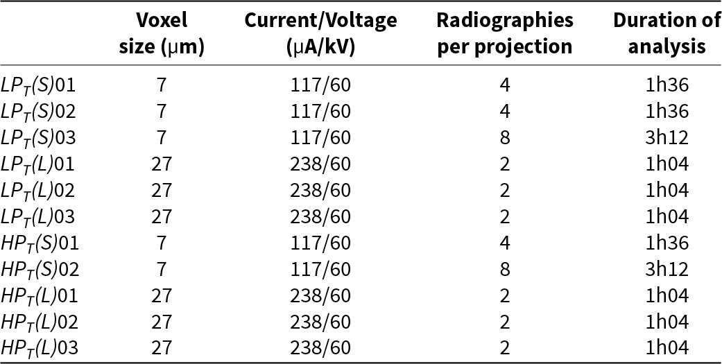

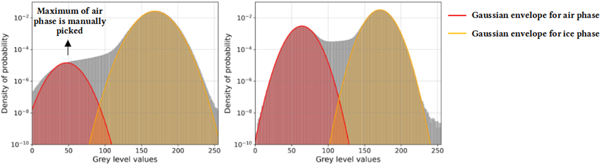
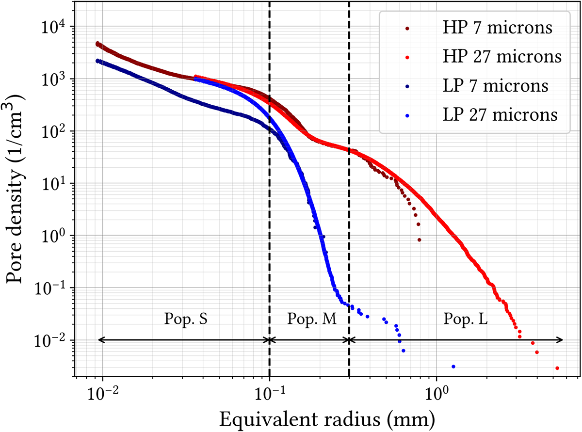

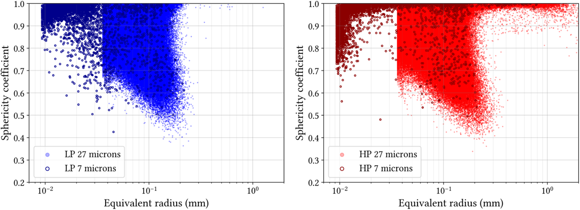
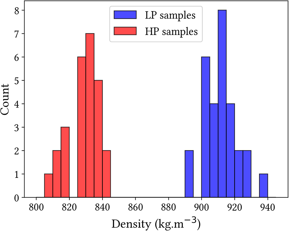


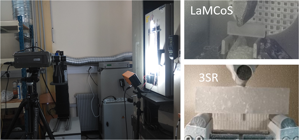
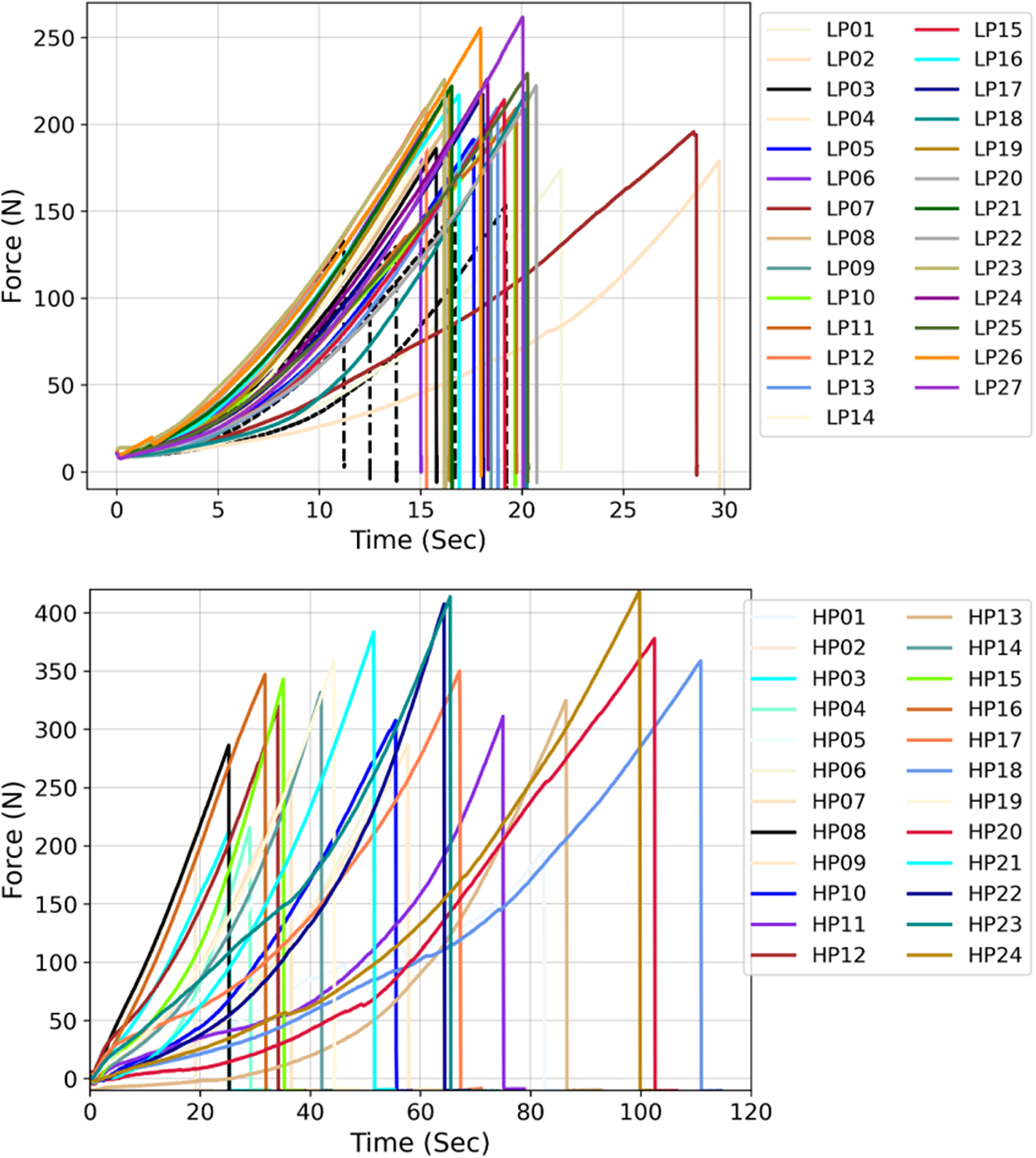
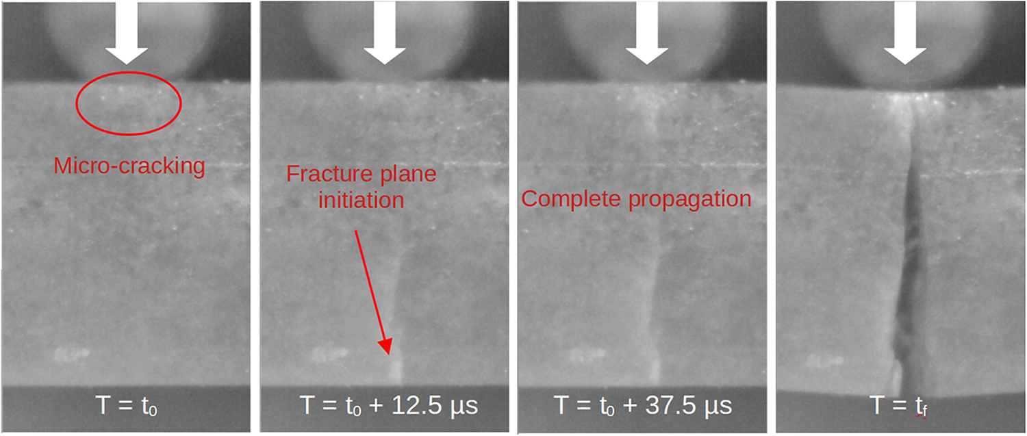
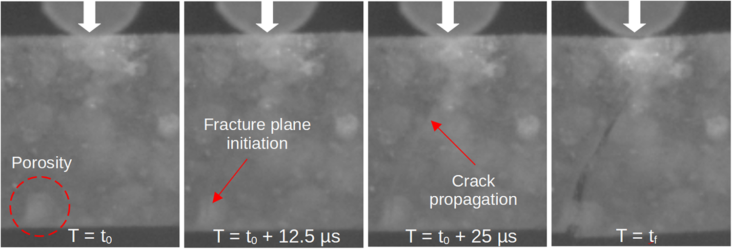
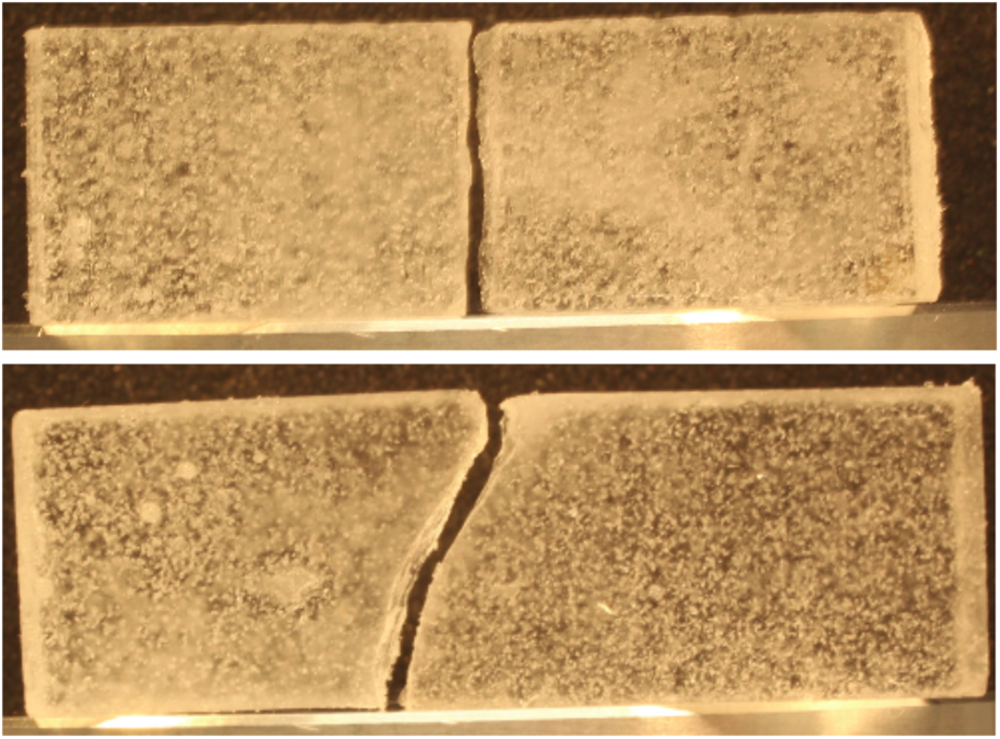
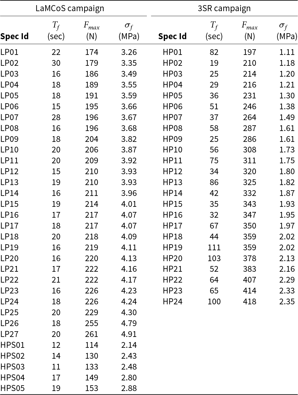


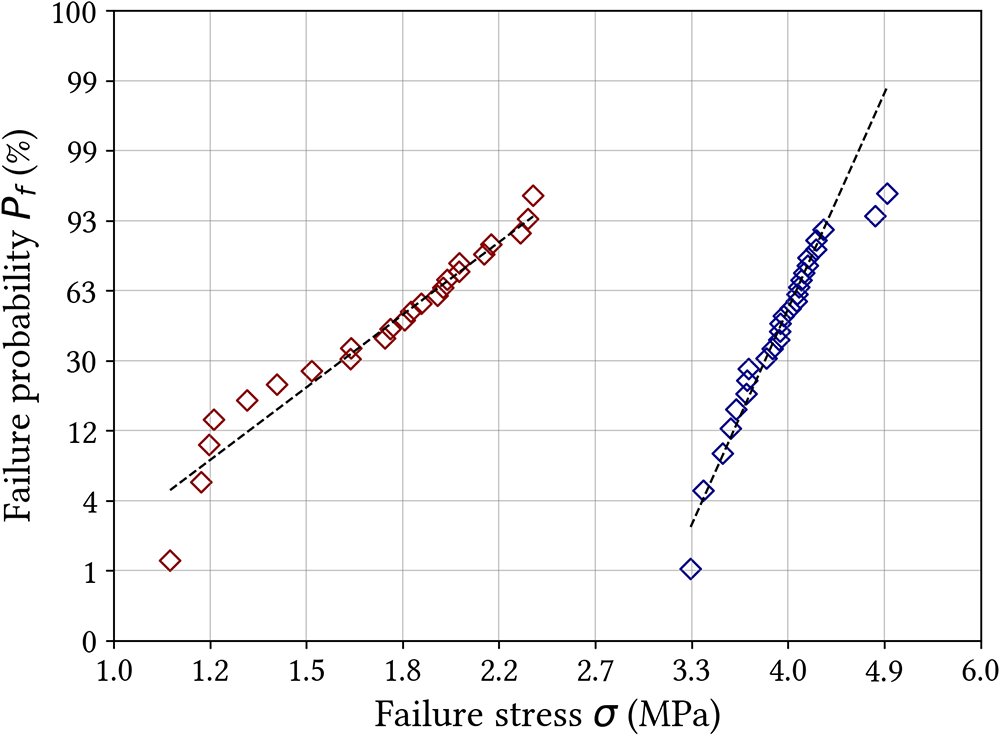
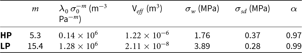


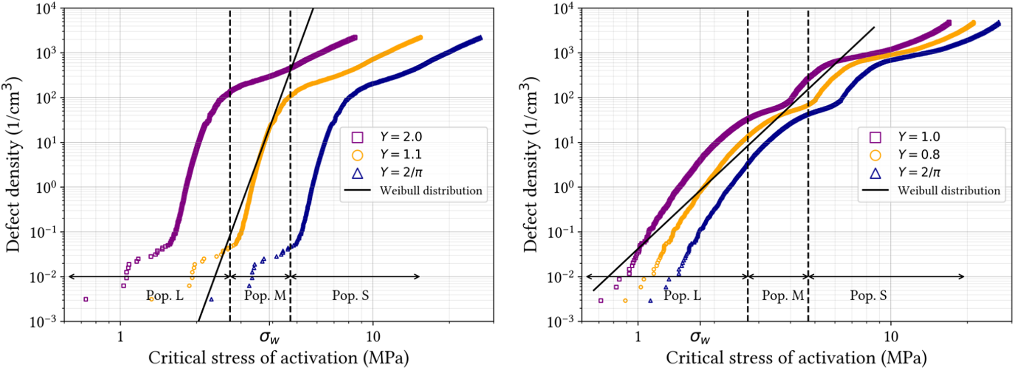


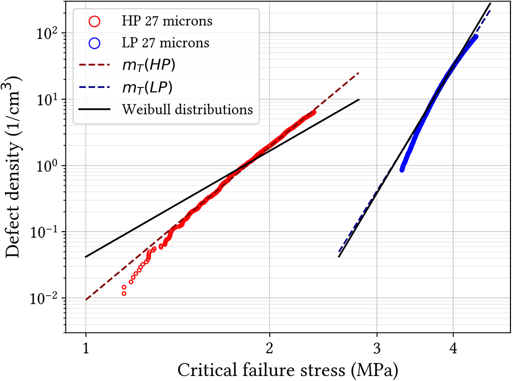

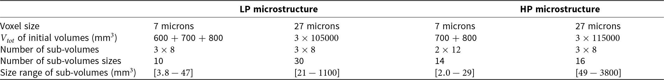

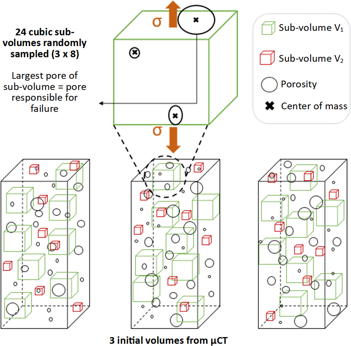
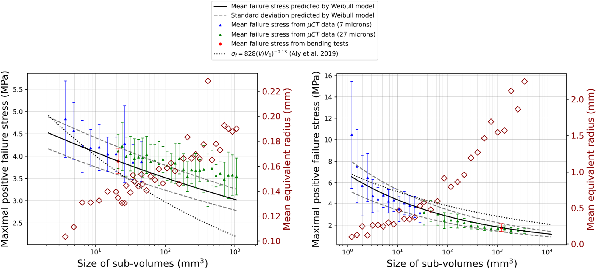


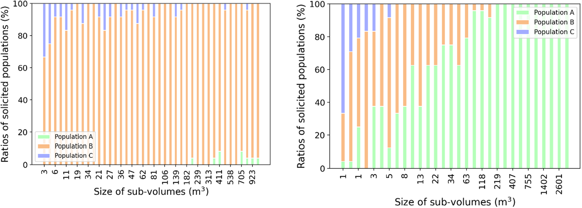

 Open access