


1. Introduction
Ice shelves are the floating extensions of ice sheets and provide resistance to the flow of grounded ice upstream. This is known as ice-shelf buttressing. The magnitude of buttressing is determined by the viscous deformation of the ice shelf, which is dependent on: the geometry of the ice-shelf embayment; the location of pinning points within the shelf; the ice-shelf thickness (controlled by ice-shelf flow, surface and basal mass balance); ice-shelf extent (controlled by the position of the calving front and iceberg calving); ice rheology and structural integrity (controlled by ice temperature, damage and crevassing).
Ice-shelf thinning in key locations, such as near grounding lines (the boundary at which ice begins to float) and in shear margins, has been shown to decrease ice-shelf buttressing in numerical ice-flow models (Reese and others, Reference Reese, Gudmundsson, Levermann and Winkelmann2018; Goldberg and others, Reference Goldberg, Snow, Gourmelen, Kimura and Millan2018). Observations show that the collapse of ice shelves, and therefore the removal of buttressing, can lead to a rapid speed up and thinning of the grounded ice upstream (Rack and Rott, Reference Rack and Rott2004; Rignot and others, Reference Rignot2004; Scambos and others, Reference Scambos, Bohlander, Shuman and Skvarca2004).
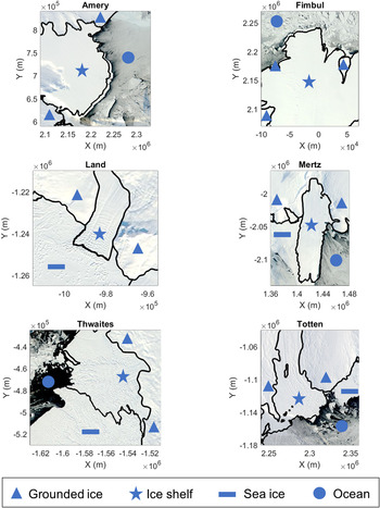
Ice shelves are often found within embayments and are rarely observed to advance substantially outside of a lateral confinement. A small number of ice tongues (unconfined ice shelves) do exist and appear to be partially supported and prevented from collapsing by the presence of landfast sea ice for much of the year (see Fig. 1 and S7) (Cuffey and Paterson, Reference Cuffey and Paterson2010, p. 127).
Worldview imagery of Amery, Fimbul, Land, Mertz, Thwaites and Totten ice shelves showing the extent of the laterally confined and unconfined regions of each ice shelf along with sea ice cover in April 2009. The grounding line and ice-ocean boundary are denoted by a black line, with regions of grounded ice, ice shelf, open ocean and sea ice denoted with symbols shown in key. Coordinates are given in WGS 84/Antarctic Polar Stereographic, with origin at the South Pole.

The extent of present-day ice shelves providing significant buttressing has been determined by Fürst and others (Reference Fürst2016). In this work, areas of ice shelves that provide little or no buttressing are classed as areas of passive ice that could be removed without triggering a significant increase in ice flow across the grounding line. These areas are consistently found close to the present-day calving front, often where the ice shelf begins to protrude out past the lateral confinement of pinning points. The buttressing number – a measure of resistance provided by the ice shelf – was used to inform the design of numerical ice-flow experiments to determine the extent of passive ice. Contours of maximum buttressing number were used to incrementally remove sections of the ice shelf in the model, while the instantaneous change in grounding-line flux determined whether these regions were deemed passive (Fürst and others, Reference Fürst2016).
There is a long held assumption that unconfined ice shelves provide no buttressing and often ice-sheet models ignore the effects of unconfined ice shelves (Cuffey and Paterson, Reference Cuffey and Paterson2010, p. 385). One mechanism by which unconfined ice shelves can theoretically generate buttressing is through hoop stresses (Morland and Zainuddin, Reference Morland, Zainuddin, Van Der Veen and Oerlemans1987; Pegler and Worster, Reference Pegler and Worster2012, Reference Pegler and Worster2013). Hoop stresses are the viscous resistance to lateral spreading in a diverging flow. They act perpendicular to the flow direction and thickness gradient, and must be overcome in order for the flow to diverge. Therefore, along-flow extension is reduced in comparison with the equivalent 2D non-diverging case (see the Theory section below for a full explanation).
Morland and Zainuddin (Reference Morland, Zainuddin, Van Der Veen and Oerlemans1987) considered the potential of an ice shelf bordering the whole of the Antarctic Ice Sheet to provide buttressing via hoop stresses. This geometry had an origin at the centre of the continent and a radius of curvature corresponding to the average distance to the ice-sheet grounding line. They concluded that at this large radius of curvature the effect of buttressing from hoop stresses would be insignificant. They overlooked the fact that it is possible for individual ice shelves to have a much smaller radius of curvature as they leave the lateral confinement of final pinning points. However, observations of unconfined ice shelves in Antarctica indicate that ice shelves do not advance large distances into open ocean. This raises two questions: Do unconfined Antarctic ice shelves provide buttressing? Can hoop stresses allow ice shelves to regrow or advance beyond lateral confinements?
We build on results from theoretical work (Morland and Zainuddin, Reference Morland, Zainuddin, Van Der Veen and Oerlemans1987; Pegler and Worster, Reference Pegler and Worster2012, Reference Pegler and Worster2013) and fluid-mechanical laboratory experiments (Pegler and Worster, Reference Pegler and Worster2012, Reference Pegler and Worster2013) that demonstrate how ice-shelf hoop stresses can provide buttressing. We present the theory, from Morland and Zainuddin (Reference Morland, Zainuddin, Van Der Veen and Oerlemans1987), Pegler and Worster (Reference Pegler and Worster2012, Reference Pegler and Worster2013), modify this for application to downstream-unconfined sections of ice shelves and explore the controls on the magnitude of buttressing using idealised examples. Using these theoretical tools we analyse the flow field of present-day unconfined sections of Antarctic ice shelves. We infer that in general these areas have low effective viscosity, most probably due to the high density of fractures within these regions, and as such are unable to sustain the high azimuthal stresses required to generate significant buttressing. However, where ice shelves are additionally stabilised by sea ice, it appears the shelf has higher effective viscosity and azimuthal stresses can be generated to provide buttressing. This suggests that sea ice may prevent an ice tongue from collapsing and potentially allows it to advance.
2. Theory: buttressing and hoop stresses
The theory of hoop-stress buttressing has been presented previously by Morland and Zainuddin (Reference Morland, Zainuddin, Van Der Veen and Oerlemans1987), Pegler and Worster (Reference Pegler and Worster2012, Reference Pegler and Worster2013). Here we present a consolidated version of this, with modification for application to the analysis of geophysical data from Antarctic ice shelves. The stresses within an ice shelf can be approximated using the Shallow Shelf Approximation (Morland, Reference Morland, Van der Veen and Oerlemans1987; MacAyeal, Reference MacAyeal1989; Pegler and others, Reference Pegler, Lister and Worster2012), under the assumption of small gradients in ice thickness, such that the 2D depth-integrated horizontal force-balance is

Here ∇ is the horizontal component of the gradient tensor, μ is the effective viscosity given by Glen's Flow Law, H is the ice-shelf thickness, u is the horizontal component of the ice velocity, e is the strain-rate tensor, ρ is the density of ice and g′ is the reduced acceleration due to gravity. (g′ = (1 − (ρ/ρw)) g, with ρ w the density of seawater and g the full acceleration due to gravity.) The first term on the left hand side (LHS) is the horizontal gradient in the vertically-integrated isotropic stress (or pressure) within the ice shelf, while the second term on the LHS is the divergence of the vertically-integrated deviatoric stress. The sum of these terms is balanced by the horizontal gradient in the vertically-integrated hydrostatic pressure difference between the ice and the ocean, which acts to drive ice flow in the direction of decreasing H.
We now consider three fundamental geometries of ice-shelf flow; a one-dimensional flowline, a laterally-confined ice shelf and a non-confined radially-spreading ice shelf.
2.1. Base case: 1D flowline model – no buttressing
First consider a simple one-dimensional approximation to an ice shelf with the domain aligned along a flowline. This simple case has been considered by many previous authors (e.g. Schoof, Reference Schoof2007; Robison and others, Reference Robison, Huppert and Worster2010) and we include it here as the first-order representation of an ice shelf. Here ice-shelf thickness and velocity vary in one dimension only (Fig. 2a). In this case, the horizontal force-balance Eqn (1) reduces to

with x aligned in the flow direction. This equation can be integrated along the length of the shelf, from the calving front, x C back to any point within the ice shelf, x i, (most commonly the grounding line, x G) to determine the depth-integrated horizontal stress at that point,

where in each term variables are evaluated at x C or x i as denoted by the vertical bar to the right of each term. The depth-integrated horizontal stress at the calving front is equal to the hydrostatic pressure difference between the ice and the ocean

Therefore, the two terms cancel in Eqn (3), giving

The extensional stress at point x i in the presence of this 1D ice shelf is equivalent to the extensional stress felt in the absence of the shelf. We consider this to be the base state in which no buttressing is generated by the ice shelf, and hence denote the depth-integrated stress F 0. The following two sections describe fundamental ice-shelf geometries that generate buttressing.
Fundamental ice-shelf geometries: (a) 1-D flowline. (b) Laterally confined ice shelf in a parallel embayment. (c) Axisymmetrical radially-spreading shelf. (d) Sector of an axisymmetric radially-spreading shelf, which in plan view forms an annulus.

2.2. Laterally confined ice shelf – shear-stress buttressing
Consider an ice shelf laterally confined within a parallel embayment. Ice flow is parallel to the side walls, aligned in the x-direction only, with y aligned perpendicular to flow. The ice-shelf thickness, H, is uniform across the width of the shelf (i.e. H(x, y) ≡ H(x)) (Pegler and others, Reference Pegler, Kowal, Hasenclever and Worster2013; Kowal and others, Reference Kowal, Pegler and Worster2016; Pegler, Reference Pegler2016; Wearing, Reference Wearing2016; Haseloff and Sergienko, Reference Haseloff and Sergienko2018), as shown in Figure 2b. The horizontal force-balance Eqn (1) reduces to

The additional term on the LHS is due to shear within the shelf, induced by friction or no-slip at the side walls of the embayment. Integrating along the length of the shelf


In this case, the depth-integrated horizontal stress, F, is reduced in comparison with the base case because of buttressing from shear stress, F shear.
The level of ice-shelf buttressing can be quantified using the buttressing number (Gudmundsson, Reference Gudmundsson2013),

B N is the difference between the depth-integrated horizontal stress in the absence of an ice shelf, F 0, and the actual depth-integrated horizontal stress F, normalised by F 0. While the value of F 0 is the same in all directions, the orientation of F must be defined. At the grounding line, the depth-integrated horizontal stress of interest acts perpendicular to the grounding line. In this case, with F aligned perpendicular to the grounding line, B N = 0 signifies that there is no buttressing generated by the shelf, while B N = 1 implies that the downstream ice shelf provides complete buttressing such that extensional stress is zero.
The buttressing number can also be used to determine buttressing within the ice shelf. In this work we consider buttressing in the flow direction (flow buttressing Fürst and others (Reference Fürst2016)) and calculate the difference between F and F 0, where F is aligned with flow. In contrast, Fürst and others (Reference Fürst2016) used the orientation and magnitude of the depth-integrated second principal stress (SPS) to define the maximum buttressing number within the ice shelf. The SPS is often not aligned in the flow direction (much of the time it is aligned perpendicular to the flow). If a section of the shelf is removed via calving, the flow and stress field within the shelf would be altered. Therefore, although B N aligned with the SPS within the ice shelf may be a useful way to choose which sections of an ice shelf to remove in a numerical model, the corresponding value of B N does not signify the magnitude of buttressing generated to resist ice flow upstream. As such, in Fürst and others (Reference Fürst2016) the maximum buttressing number varies between each section of passive ice. It is an open question whether a buttressing number is an effective way to measure buttressing within ice shelves, where flow and stress fields may be complex. We avoid this issue by considering simple geometries where the flow is perpendicular to the grounding line, such that buttressing in the flow direction acts across the grounding line. We use the flow buttressing number throughout the following analysis and hereafter refer to this as the buttressing number, B N.
2.3. Unconfined radially-spreading ice shelf – hoop-stress buttressing
The third fundamental configuration we consider is an unconfined ice shelf, which is able to spread laterally in two directions. The simplest idealised example of this is an ice shelf spreading from a point source. In cylindrical coordinates, with the source at the origin, the flow is radially outwards and axisymmetric (symmetric with respect to rotation around the vertical axis) (Fig. 2c). This type of geometry has been considered previously by Morland and Zainuddin (Reference Morland, Zainuddin, Van Der Veen and Oerlemans1987), Pegler and Worster (Reference Pegler and Worster2012, Reference Pegler and Worster2013). With the radial coordinate, r, aligned in the flow direction and no variation in flow azimuthally (with respect to rotation about the vertical axis), the force-balance Eqn (1) becomes

The full derivation of this equation is given in Appendix A. The first term on the LHS is the radial derivative of the vertically-integrated isotropic stress and along-flow (radial) deviatoric stress (identical to the LHS of Eqn (2), but in cylindrical coordinates). The second term on the LHS of (12) is the depth-integrated radial gradient in the azimuthal strain rate, multiplied by the effective viscosity. This is the additional component from the divergence of the strain-rate tensor, which emerges in cylindrical coordinates, and is required to ensure the flow is incompressible when the shelf flows radially (Appendix A). Equation (12) can be integrated radially back from the ice front (r C) to a point in the ice shelf (r i) to give


as in Pegler and Worster (Reference Pegler and Worster2012). Therefore, hoop stresses make a positive contribution to buttressing where the azimuthal extension u/r exceeds the radial extension ∂u/∂r. Conversely, negative hoop-stress contributions are made where azimuthal extension is less than radial extension. When the hoop-stress buttressing is negative the viscous resistance to azimuthal extension acts to increase radial extension and pulls ice downstream. From the integrand it is clear that the magnitude of hoop-stress contributions increases for increasing effective viscosity (μ) and thickness (H), but decreases with a radial distance.
Physically, hoop stresses act as the viscous resistance to spreading in the azimuthal direction as the ice shelf flows radially. For an axisymmetric shelf there is no azimuthal thickness gradient, so azimuthal spreading must be induced by the radial thickness gradient. As with the shear-stress case, the integrated effect of this viscous deformation back from the ice front produces buttressing and may reduce the extensional stress at the grounding line.
For an axisymmetric ice shelf extending to infinity, Pegler and Worster (Reference Pegler and Worster2012) established analytically an upper bound for the radius of curvature at the grounding line that would provide positive buttressing; $L \equiv \lpar \mu Q_0/2 \pi \rho g^{\prime} H_0^{2}\rpar ^{1/2}$ , where H 0 and Q 0 are the ice thickness and flux at the grounding line. Pegler and Worster (Reference Pegler and Worster2012) estimated that for a typical ice shelf L ≈ 5 km. Furthermore, for ice shelves with radius of curvature at the grounding line greater than 6L, hoop stresses provided negative buttressing – generating additional extension at the grounding line. This analytical work was accompanied by laboratory-scale analogue experiments.
Here we consider hoop-stress buttressing generated by unconfined sections of ice shelves of finite length, found where ice shelves flow out past lateral pinning points, such as Amery and Fimbul Ice Shelves, Figure 1. The downstream sections of these ice shelves can be approximated as sectors of an annulus with radius of curvature at the upstream boundary (r E) dependent on the lateral divergence of the flow, Figure 3. With no shear against lateral boundaries, these sections can be approximated as azimuthally symmetric. We first consider some idealised examples, determining the magnitude of hoop-stress buttressing produced in each case. Then, using geophysical, data we assess hoop-stress buttressing in unconfined sections of Antarctic ice shelves.
Approximating an unconfined section of an ice shelf as an annulus diverging from an imaginary origin (r = 0). The ice shelf flows out from an area of confinement and diverges into open ocean. The radius of curvature at the exit of the embayment (r E) and at the calving front (r C) are labelled.

3. Idealised examples
We model the unconfined downstream section of an ice shelf, with geometry resembling a sector of an annulus in plan-view, as shown in Figures 2d and 3. We assume there is no azimuthal variation in flow or ice thickness so consider a radial flowline. We denote an imaginary origin, r = 0, from which we determine positions r E and r C, as the radius of curvature at the upstream boundary (exit of the embayment) and the ice front respectively. We impose a fixed ice thickness and velocity at r E, and balance extensional stress with the vertically-integrated hydrostatic pressure difference between the ice and ocean at the calving front r C. We assume a Glen's Flow Law rheology

with rate factor A = A −10 = 3.5 × 10⁻²⁵ s−1 Pa−3, appropriate for ice at −10° C (Cuffey and Paterson, Reference Cuffey and Paterson2010), n = 3 the flow-law exponent and eII the second invariant of the strain-rate tensor. Simulations are initiated with an ice shelf of uniform thickness. We solve Eqn (12) numerically using successive over relaxation (Young, Reference Young1971) to determine the radial velocity and then evolve the thickness of the ice shelf according to the continuity equation

where b is the net specific mass balance; the sum of surface accumulation and ablation, and basal melting and freeze-on. The thickness is evolved forward in time using an explicit time-stepping scheme until a steady state is reached. We calculate the buttressing from hoop stresses produced in the shelf downstream of r E. For these idealised examples we set b = 0.
3.1. Example 1
Figure 4 shows the steady-state results for an ice shelf of length 50 km, with radius of curvature at the upstream boundary of 70 km. The input thickness is 400 m and the input velocity is 500 m a−1. For an angle of divergence of 10°, the shelf diverges from a width of 20 to 40 km along its length. Throughout the shelf the azimuthal strain rate is greater than the radial strain rate, implying a positive hoop-stress contribution everywhere. This can been seen from the increase in the buttressing number back from the calving front to r E where it reaches 0.2; i.e. 20% of the hydrostatic stress is balanced by hoop stresses.
Example of an idealised ice shelf with rate factor A −10. The radius of curvature at the upstream boundary is 70 km and shelf has a length of 50 km. (a) Ice speed. (b) Ice-shelf thickness profile (blue) and value of the local thickness-profile exponent, a (red), for function $H=\tilde {H}r^{-a}$ , calculated at each point by fitting the function to an 11-km interval around each point. (c) Radial strain rate (blue), azimuthal strain rate (red), difference; radial minus azimuthal strain rate (orange). (d) Depth-integrated stresses; radial extension (blue), hydrostatic driving stress (red dashed) and hoop stress (dotted yellow). (e) Buttressing number along the length of the shelf.

3.2. Example 2
A similar shelf is shown in Figure 5, however the radius of curvature at the upstream boundary has been increased to 400 km and the shelf is now 100 km long. Due to the large radius of curvature the width of the shelf only increases from 140 to 170 km along its length, for an angle of divergence of 10°. Figure 5c shows that the azimuthal strain rate is greater than the radial strain rate in the downstream section of the shelf (>435 km) only. This leads to a transition from positive to negative hoop-stress buttressing contributions in the upstream direction. The peak in buttressing number is just downstream of this transition (Fig. 5e) because the ice is thinner and the driving stress (hydrostatic pressure difference between ice and ocean) decreases downstream. In this case the buttressing number at the upstream boundary (r E = 400 km) is very small and the shelf provides insignificant buttressing via hoop stresses (<1.5%).
Same as Figure 4, but with a 400 km radius of curvature at the upstream boundary and shelf of 100 km in length. Hoop-stress buttressing remains positive throughout the length of the shelf. However, negative hoop-stress contributions are made in the upstream section and hence the peak in hoop-stress buttressing is located at r ≈ 440 km.

3.3. Positive and negative hoop-stress contributions
For steady-state ice shelves the sign of the hoop-stress buttressing contribution is dependent on the local ice-shelf thickness profile. For a radially spreading shelf, with angle of divergence θ at the origin, the flux at radius r in the steady state is

where q 0 is the input flux at r = 0 and the second term on the RHS is the net mass gain/loss between the origin and r, due to surface or basal processes. The ice must thin in the downstream direction and we approximate the local ice thickness profile as

where the exponent a is dependent on the local curvature of the ice thickness and in turn the deformation of the shelf at this point. Therefore the radial velocity takes the form

This can be used to determine the radial and azimuthal strain rates, such that hoop-stress buttressing contributions are positive when


In the case of b = 0, this reduces to a < 2. Therefore, in the steady-state with b = 0, at locations where the ice thickness profile can be approximated by $\tilde {H} r^{-a}$ with a < 2, positive hoop-stress buttressing is generated. The exponent for the local ice-thickness profile, a, is calculated at each point along the shelf using the MATLAB curve fitting function fit, which uses the ice thickness within an 11 km interval centred at each point to determine a. The spatially-evolving value of a is shown in Figure 5b, where there is a transition from a > 2 to a < 2 at r ≈ 435 km, where the magnitude of the radial and azimuthal strain rates are equal. For a > 2 hoop-stress buttressing contributions are negative. In contrast, in Figure 4b, hoop-stress contributions are positive throughout the length of the shelf and a < 2 everywhere.
3.4. Varying parameters
As identified by Pegler and Worster (Reference Pegler and Worster2012), the magnitude of buttressing from hoop stresses is dependent on the radius of curvature at r E, the shelf viscosity, the input thickness and input velocity. In Figure 6 these parameters, along with the length of the ice shelf, are varied to assess the impact on buttressing.
Varying parameters in the idealised model. Each panel shows the buttressing number (vertical axis): (a) along the length of the shelf when increasing the shelf length; (b) at the upstream boundary (r E) of a 75 km shelf, when the radius of curvature at the upstream boundary (r E; horizontal axis) and rate factor (A X; coloured curves) are varied; (c) and (d) along the length of the shelf for varying input thicknesses (fixed velocity 500 m a−1) (c) and varying input velocities (fixed thickness 400 m) (d).

As the length of a shelf is increased the buttressing number at r E increases (Fig. 6a). However, the magnitude of this increase decreases with shelf length, and the peak in buttressing number is shifted downstream. This implies that hoop-stress buttressing increases at a reduced rate in comparison with the driving hydrostatic pressure as the ice thickens (it is the ratio of hoop-stress buttressing to driving stress that determines the buttressing number). It may also suggest that the upstream section of the shelf begins to produce negative hoop-stress contributions. However, further assessment shows that in these cases the azimuthal extension remains larger than radial extension and the thickness-profile exponent a remains less than 2. Therefore, hoop-stress contributions remain positive.
Figure 6b shows the effects of varying both the radius of curvature at the upstream boundary and the rate factor for an ice shelf of fixed length (75 km). Buttressing is reduced as the radius of curvature at the upstream boundary, r E, increases and the lateral divergence of the shelf decreases. There is a transition to slightly negative buttressing once r E increases past a critical point. This is dependent on the rate factor in the ice rheology. For decreasing rate factor, and therefore increasing effective viscosity, hoop stresses provide greater buttressing.
Figures 6c and d show the buttressing number for varying input fluxes at the upstream boundary. Increasing the input thickness and maintaining input velocity leads to reduced buttressing. This is because thicker ice produces a larger driving stress, which generates large radial strain rates. Conversely, for a fixed input thickness and increased input velocity, buttressing increases. This is because the hydrostatic driving stress remains the same, but the azimuthal strain rate increases like u/r.
4. Hoop-stress buttressing from Antarctic ice shelves
We now use this theory to approximate the magnitude of hoop-stress buttressing generated by unconfined Antarctic ice shelves.
4.1. Method
We approximate the unconfined section of each ice shelf as an annulus using ice-surface velocities and the divergence of flowlines to determine the geometry. We then model the ice flow within the annulus, as in the previous section, to estimate the hoop-stress contribution to buttressing. The process is detailed in Appendix B and summarised here. A geometric argument is used to determine upstream, downstream and lateral boundaries along with the radius of curvature. We used a Gaussian smoothed version (Wearing and others, Reference Wearing, Hindmarsh and Worster2015; Wearing, Reference Wearing2016) of MEAsUREs V2 surface velocity data (Rignot and others, Reference Rignot, Mouginot and Scheuchl2011, Reference Rignot, Mouginot and Scheuch2017) and Bedmap2 ice thickness data (Fretwell and others, Reference Fretwell2013).
Flowlines are used to identify the lateral extent of the spreading ice shelf once it leaves lateral confinement. We draw lines perpendicular to the approximate central flowline at the upstream and downstream extent of this unconfined region to mark the position of the upstream and downstream boundaries. We draw two additional lines connecting the outermost points of the upstream and downstream boundaries and extend them upstream until they intersect. This defines the imaginary origin and the radius of curvature at the upstream and downstream boundaries. The ice thickness and speed at the boundaries are determined by the mean along each boundary. Assuming steady state, we estimate the mean specific mass balance, $\bar {b}$ , over the unconfined area of the shelf using the difference in flux across the upstream and downstream boundary.
Once the geometry, input flux and specific mass balance are known, we use the radial force-balance Eqn (12) and continuity Eqn (18) (with $b= \bar {b}$ ) to model the thickness profile, velocity field and hoop-stress buttressing. We begin with a uniform thickness ice shelf (equal to the average ice thickness at the upstream boundary) and the shelf is evolved to steady state. The process is repeated for three different rate factors in the rheological model, A = A −2, A −5 and A −10, with subscripts denoting appropriate ice temperature in degrees Celsius (Cuffey and Paterson, Reference Cuffey and Paterson2010). The final ice thickness and speed profiles are compared to the data along six flowlines. The root mean square error (RMSE) is calculated between the model output and the flowline data, with the mean of the RMSEs used to determine which rheology provides the best fit. We restrict analysis to six ice shelves of varying sizes that clearly extend beyond lateral confinements: Amery, Fimbul, Land, Mertz, Thwaites and Totten.
Alternative approaches for determining hoop-stress buttressing may be possible. For example, using velocity data along streamlines to compute hoop-stress contributions directly. However, differentiating the often noisy data generates sharp fluctuations in strain rates, which impede interpretation of the results. (An outline of this method and some preliminary results are shown in the Supplementary Material (SM) and Wearing, Reference Wearing2016.) Alternatively, a formal inversion procedure could be used to simulate the stress field and assess hoop-stress buttressing. However, the simplicity of our approach aids our understanding of the controls on hoop-stress buttressing and our conclusions do not rely heavily on a fully resolved stress field.
4.2. Results
Figure 7 shows results from Amery Ice Shelf. The radius of curvature at the upstream boundary is approximately r E = 150 km, with a further 55 km of unconfined ice shelf downstream. The best fit to the flowline data of ice thickness and speed is achieved for an idealised ice shelf with rate factor A −5 (Figs 7b, c). Hoop-stress buttressing contributions are positive throughout the shelf; i.e. azimuthal strain is greater than radial strain (Fig. 7d, dashed curves for A −5). For a weaker rheology, A −2, this is not the case, with negative hoop-stress contributions in the upstream part of the shelf (Fig. 7d, dotted curves for A −2). The buttressing number at the upstream boundary is approximately 0.04. This relatively small buttressing number is due to the large radius of curvature at the upstream boundary and the low rate factor which leads to low effective viscosity.
Applying idealised model annulus to Amery Ice Shelf: (a) ice speed map with geometry of flowlines and upstream and downstream boundaries. (b) Flow speed along flowlines 1 - 6 (bottom to top in (a)) (dashed curves) with simulated speed (solid curves) at three rate factors (A −2, A −5 and A −10). (c) Same as (b) but for ice thickness. In both (b) and (c) the mean RMSE for each rate factor is given in the brackets in the legend. (d) Strain rates from model and (e) buttressing number along length of shelf. In (d) and (e); A −2 (dotted), A −5 (dashed) and A −10 (solid).

The buttressing numbers from the upstream boundary, r E, downstream to the calving front for each of the ice shelves considered are shown in Figure 8 with a complete set of plots for each ice shelf, as for Amery Ice Shelf in Figure 7, given in the SM (Figs S1–S6). The buttressing number is shown for three rate factors (A −2, A −5 and A −10) with thick blue curves corresponding to results with the smallest mean RMSE between the model and the flowline velocity and thickness.
Buttressing number along the length of unconfined section of ice shelves: Amery, Fimbul, Land, Mertz, Thwaites and Totten. Buttressing numbers are shown for all rate factors, with bold blue curves, corresponding to the models with speed and ice thickness that best match data (the best match is different for speed and thickness in panel (f), so there are two blue curves). In the legend the mean RMSE for the speed (S) and ice thickness (H) are shown in brackets for each rate factor. See Figures S1–S6 for full set of plots as in Figure 7.

Fimbul Ice Shelf has a very large radius of curvature as it flows beyond the final lateral pinning points, r E = 320 km, and an unconfined shelf of 50 km in length. The buttressing number at the upstream boundary is approximately 0.04, for rate factor A −10, suggesting insignificant buttressing (Fig. 8b). This is largely due to the large radius of curvature, which implies low azimuthal spreading and therefore little buttressing despite colder and therefore more viscous ice.
Land Ice Shelf, Figure 8c, is a relatively small ice shelf with an unconfined section of 8 km in length, and a radius of curvature of 32 km at the upstream boundary. Here it is unclear which rheological parameters provide the best fit to the data, as ice-shelf flow increases along all flowlines, but the ice thickness appears to thin along some and thicken along others (Figs S3b, c). This uncertainty leads to a large range in potential buttressing numbers at the upstream boundary between 0.04 and 0.15. However, the lowest mean RMSE is achieved for rate factor A −2, with buttressing 0.04.
For Mertz Ice Tongue, Figure 8d, rate factors between A −5 and A −10 appear to be most appropriate (Figs S4 b, c). The smallest mean RMSE is obtained for A −10 with a buttressing number at the grounding line of 0.09, produced by a shelf of length 29 km and r E = 101 km.
For Thwaites Glacier Ice Shelf (r E = 230 km and length 30 km) the best match between velocity, thickness and the idealised model is for ice with A −2 (Fig. S5). However, this fit could be improved further with an even weaker rheology. This suggests the shelf is made up of very weak ice. This can also be inferred from the high density of visible surface fractures on the shelf Figure 1. In this case hoop-stress buttressing from the ice shelf is very small and potentially negative at the upstream boundary.
The best match between the idealised model and flowline data for Totten Ice Shelf is achieved for relatively warm ice temperatures; A −2, A −5, with RMSE values lowest for the ice flow speed and ice thickness respectively. This leads to buttressing numbers at the upstream boundary of between 0.01 and 0.03.
5. Discussion
For most of the ice shelves analysed, except Mertz Ice Tongue (and possibly Land Ice Shelf), hoop-stress buttressing from the unconfined section of the ice shelf produces insignificant buttressing, with buttressing numbers less than 0.05; buttressing from hoop stresses balances less than 5% of the driving stress. This is due to weak rheology and large radii of curvature. None of the ice shelves assessed produce negative hoop-stress buttressing, with the exception of Thwaites Ice Shelf, which potentially produces insignificant negative buttressing (<0.5%). In the case of Amery and Totten ice shelves, the geometry of the divergent flow has the potential to provide hoop-stress buttressing of approximately 10% of the radial driving stress if the ice had a larger rate factor (i.e. A −10 or more). In general, the rheological parameters that produce the best fit to geophysical data are appropriate for warm ice ($A=A_{-5}\comma\; A_{_2}$ ), with temperatures greater than would normally be expected for ice shelves (depth-averaged englacial temperatures are typically less than or equal to −5°C; Fig. S8). This suggests that the ice is weakened by damage such as fracturing and crevasses (Borstad and others, Reference Borstad2016).
We hypothesise that most unconfined Antarctic ice shelves are unable to provide buttressing of greater than 0.05 because they are unable to sustain the large azimuthal stresses required without the formation of fractures that weaken the ice. For substantial hoop-stress buttressing the azimuthal strain rate needs to be significantly larger than the radial strain rate. For typical radial strain rates of 0.01 a−1 with a rate factor A −10 this leads to stresses on the order of 75 kPa. Stresses larger than this are likely to generate fractures (Vaughan, Reference Vaughan1993) and once fractures are initiated the ice can no longer support such large stresses (Borstad and others, Reference Borstad2016). In addition, laboratory-scale fluid-mechanical experiments have shown that radially-flowing shear-thinning fluids (Glen's flow law implies ice is shear thinning) produce radial fractures (Sayag and others, Reference Sayag, Pegler and Worster2012).
Ice shelves with larger buttressing from hoop-stresses, such as Land and Mertz, form ice tongues that are potentially further stabilised by sea ice for much of the year. Figure 1 shows the unconfined regions of each ice shelf in April 2009 at the end of the austral summer (this year corresponds to when the majority of the velocity data were collected; Rignot and others, Reference Rignot, Mouginot and Scheuchl2011, Reference Rignot, Mouginot and Scheuch2017). Equivalent plots for September 2009 are shown in SM; Figure S7. In both periods extensive regions of landfast sea ice are visible around Land and Mertz ice shelves. In our modelling, these shelves have lower rate factors (A −10) and small radii of curvature allowing more substantial buttressing from hoop stresses. As seen from the theoretical examples, buttressing increases for increased ice viscosity and decreased radius of curvature at the upstream boundary.
Despite the potential for hoop stresses to generate buttressing in unconfined ice shelves, our findings support those of Fürst and others (Reference Fürst2016), who concluded that these regions should be classed as passive. However, buttressing of 10% or greater could be achieved for unconfined ice shelves that maintain a high effective viscosity, through preventing the formation of fractures and crevasses, possibly through extra stabilisation from sea ice for large parts of the year. Loss of extensive sea ice has previously been linked to accelerations in ice flow and reductions in ice-shelf extent (Miles and others, Reference Miles, Stokes and Jamieson2017; Greene and others, Reference Greene, Young, Gwyther, Galton-Fenzi and Blankenship2018; Massom and others, Reference Massom2018). However, we can not discount that the sea ice is providing a substantial portion of the buttressing we are attributing to hoop stresses.
There are two main limitations of this application of the hoop-stress theory to Antarctic ice shelves. Firstly, the unconfined regions at the downstream end of ice shelves do not form perfect sectors of an annulus and flowlines are not azimuthally symmetric. In particular, there is an imprint of the upstream ice thickness and speed at the transition from laterally-confined to unconfined flow. The shear of the ice shelf between lateral pinning points while the shelf is confined means that ice flow is typically fastest and ice thicker in the centre of the shelf. As a result, the calving front usually extends further in the centre of the shelf than at the flanks, leading to the calving front having a smaller radius of curvature than the annulus we consider.
Here we have taken the simplest approach in order to produce first-order estimates of the magnitude of hoop-stress buttressing generated by unconfined sections of ice shelves. One way to avoid fitting an approximate annulus geometry would be to analyse strain rates along a 2D streamtube (bounded by two streamlines) to determine the hoop-stress buttressing from lateral spreading of that streamtube. One reason that this is not effective is that our theory ignores lateral variation in flow, which may result from lateral variations in ice thickness. There is also noise in the data, which results from the compilation of multiple sets of interferometric synthetic-aperture radar and optical feature-tracking data over multiple time periods (Rignot and others, Reference Rignot, Mouginot and Scheuchl2011, Reference Rignot, Mouginot and Scheuch2017). Therefore it is not possible to make direct comparisons with the theoretical model and the physical processes that determine the observed variations of the extensional strain rate; do they result from hoop stresses, shear or noise in the data?
A second limitation that applies both to the approximate annulus and streamtube method is that in order to determine hoop stress it is necessary to know both the strain rates and effective viscosity. Strain rates can be calculated from surface velocities. Here we have used a range of rate factors in the ice rheology and considered a simple comparison between data (ice thickness and speed) along flowlines and model output in the steady state, to determine which rate factor is most appropriate. This could be improved by assimilating the ice flow in an ice-shelf model and tuning the rheological parameters to match with observed velocities (MacAyeal, Reference MacAyeal1993; Gillet-Chaulet and others, Reference Gillet-Chaulet2012; Arthern and others, Reference Arthern, Hindmarsh and Williams2015; Fürst and others, Reference Fürst2015). The stress field could then be obtained directly from the model.
However, despite these limitations, our simplified approach has several advantages over using more complex geometries to partition ice shelves or taking a data-assimilation approach. Firstly, it effectively characterises the large-scale flow structure without incorporating the presence of significant observational noise, which is problematic when computing velocity gradients. Secondly, the annulus-based approach provides insight into the fundamental controls on hoop-stresses. For example, the clear relationship between radius of curvature and contributions to hoop-stress buttressing, apparent in our numerical results, can be directly linked to the relative magnitudes of radial and azimuthal extension through Eqn (16). Moreover, given that our aim is to assess if significant hoop-stress buttressing is generated in unconfined portions of Antarctic's ice shelves, rather than quantifying buttressing, these limitations do not affect our main conclusions.
6. Conclusions
Theoretically, unconfined ice shelves can provide buttressing via hoop stresses, the viscous resistance to azimuthal extension for a radially spreading flow (Morland and Zainuddin, Reference Morland, Zainuddin, Van Der Veen and Oerlemans1987; Pegler and Worster, Reference Pegler and Worster2012, Reference Pegler and Worster2013). The magnitude of hoop-stress buttressing is dependent on the difference between the rate of azimuthal and radial spreading, the radius of curvature, the length of the unconfined ice shelf and the effective viscosity, which is dependent on the rheological rate factor and extent of ice damage. High positive hoop-stress buttressing can be produced by rapidly-diverging, thick ice shelves that have a high effective viscosity.
When we compare our results from idealised modelling with ice thickness and flow speed along flowlines, rate factors appropriate for relatively warm ice are required to best-match observations. This suggests that unconfined ice shelves consist of weak ice with a low effective viscosity, which most likely results from the presence of a large number of fractures and damaged ice. In order to contribute positively to hoop-stress buttressing, the azimuthal strain rate must be larger than the radial strain rate. For typical radial strain rates observed in Antarctic ice shelves, the required azimuthal strain rates produce extensional stresses that are at the lower bound of those that cause fracturing. Once the ice is damaged it is no longer able to sustain high extensional stresses.
We have shown that some Antarctic ice shelves can provide buttressing equal to approximately 10% of the extensional driving stress, with rate factors appropriate for ice at −10°C. These ice shelves are stabilised by the presence of sea ice, which may prevent large-scale fracturing and break-up. This suggests that the presence of sea ice is vital in order for an ice shelf to advance into open ocean, without fracturing and maintaining significant hoop-stress buttressing. Pinned sea ice may act like a preliminary ice shelf, reducing ice-fracturing. Processes of this nature may be important when considering the growth of ice sheets during glacial cycles.
Supplementary material
The supplementary material for this article can be found at https://doi.org/10.1017/jog.2019.101.
Acknowledgments
The authors would like to thank Robert Arthern for his helpful and insightful comments during the development of this work. We are also grateful for the comments from our two reviewers and the scientific editor, which helped to improve the manuscript. We acknowledge funding from NSF (award number 1743310).
APPENDIX A. Axisymmetric, radially-spreading shelf: force balance
The horizontal depth-integrated force-balance equation from the Shallow Shelf Approximation (Morland, Reference Morland, Van der Veen and Oerlemans1987; MacAyeal, Reference MacAyeal1989; Pegler and others, Reference Pegler, Lister and Worster2012), takes the form

For an axisymmetric radial flow, with no azimuthal variation in thickness or speed, spreading from an origin at r = 0, the horizontal velocity takes the form u = (u(r), 0). In cylindrical polar coordinates the strain-rate tensor is

and the divergence in the horizontal velocity is

Therefore the radial component of the force balance Eqn (A1) becomes


The first term on the LHS is the radial derivative of the vertically-integrated isotropic stress and along-flow (in this case, radial) deviatoric stress (the equivalent to Cartesian cases). The second term on the LHS is the depth-integrated radial gradient in the azimuthal strain rate, multiplied by the effective viscosity. Here the radial force-balance equation is split into two terms on the LHS: (1) the extensional terms resulting from the radial derivative of the vertically-integrated isotropic stress and the radial derivative of the radial deviatoric stress; and (2) the hoop-stress term resulting from the radial derivative of the azimuthal strain rates. These additional terms (in comparison with the Cartesian case) are included when working in cylindrical polar coordinates because the ice shelf must spread laterally in additional to radially when flowing in a divergent geometry to ensure incompressibility, Figure 9. The along-flow terms are the equivalent to those in the Cartesian case, however here an additional azimuthal component results from the divergent flow.
Schematic of incompressibility terms in a laterally confined (a) and radially spreading (b) flow.

These equations demonstrating how hoop stresses arise in radially spreading flows have been derived previously by Morland and Zainuddin (Reference Morland, Zainuddin, Van Der Veen and Oerlemans1987), Pegler and Worster (Reference Pegler and Worster2012, Reference Pegler and Worster2013).
APPENDIX B. Approximation to Antarctic ice shelves: method
We calculate flowlines and perform numerical calculations in MATLAB and determine the geometry of the annulus in ArcMap. We calculate flowlines from 10 equally-spaced points spanning the width of the ice shelf just upstream of the transition from laterally confined to unconfined, as seen in Figure 10. These flowlines are used to determine the approximate lateral extent of the ice that spreads in a manner similar to a sector of an annulus, as discussed in the main text. We draw a line perpendicular to the central flowline between the final lateral pinning points signifying the upstream boundary of the annulus. We consider the intersection of this line with the outermost flowlines of the spreading and unconfined shelf to mark the upstream lateral boundaries of the annulus. Once the geometry of the upstream boundary is established, a second set of six flowlines originating from equally spaced points along the upstream boundary are calculated, Figure 7a. The downstream boundary is marked by a second line parallel to the first, which spans the downstream limit of the flowlines before reaching the calving front. The two parallel lines and lateral flowlines form an approximate trapezium, or sector of an annulus.
Map showing the original 10 flowlines spanning the width of Amery Ice Shelf used to determine the extent of the laterally spreading region.

Two straight lines are drawn between the edges of the upstream and downstream boundaries, which are extended upstream until they intersect. Using the distance measuring tool in ArcMap, the distance from the upstream boundary to the intersection is determined giving the approximate radius of curvature at the upstream boundary. The distance from the upstream to downstream boundary is measured, as well as the length of the upstream and downstream boundaries, giving the width of the flow at these locations.
Ice thickness and speed are sampled along the flowlines. The flux across the upstream and downstream boundaries is calculated by averaging the ice thickness and speed at the intersection of each flowline with the boundary and then multiplying by the width of the flow. Assuming the shelf is in steady state, the difference between the flux over the upstream and downstream boundaries gives the volume of ice lost (or gained) through basal melting (or freeze-on and surface accumulation). The average melt (freeze-on) rate is calculated by dividing the flux difference by the area of the annulus.


 Open access