


Introduction
The Greenland ice sheet has been losing 100 to >300 Gt of ice per year in recent decades through increased surface melting and iceberg calving at marine-terminating glaciers, with calving contributing up to half of this mass loss (Enderlin and others, Reference Enderlin2014; The IMBIE Team, 2020). Marine-terminating glaciers drain inland ice to the sea, and accurate sea-level projections depend on understanding the dynamics and changes of these glaciers (IPCC, Reference Stocker2013). Over the last century, Greenland outlet glaciers have experienced increasing flow speeds and terminus retreat (Joughin and others, Reference Joughin, Abdalati and Fahnestock2004; Howat and others, Reference Howat, Joughin, Tulaczyk and Gogineni2005, Reference Howat, Joughin and Scambos2007; Luckman and others, Reference Luckman, Murray, de Lange and Hanna2006; Stearns and Hamilton, Reference Stearns and Hamilton2007), as well as increasing numbers of glacial earthquakes, which occur during capsizing of large icebergs during calving events (Ekström and others, Reference Ekström, Nettles and Tsai2006; Tsai and Ekström, Reference Tsai and Ekström2007; Nettles and Ekström, Reference Nettles and Ekström2010; Murray and others, Reference Murray2015a; Olsen and Nettles, Reference Olsen and Nettles2017). Thinning or velocity increase at marine-terminating glacier termini can propagate inland and contribute to larger-scale mass imbalance (Joughin and others, Reference Joughin, Smith and Holland2010); thus, understanding the processes occurring at glacier termini is critical to projecting glacier change in a warming world.
At many marine-terminating glacier termini, subglacial discharge plumes fed by surface meltwater enhance submarine melt and interact with iceberg calving processes (Motyka and others, Reference Motyka, Hunter, Echelmeyer and Connor2003; Fried and others, Reference Fried2015; Slater and others, Reference Slater, Nienow, Cowton, Goldberg and Sole2015; Carroll and others, Reference Carroll2016; Schild and others, Reference Schild2018; How and others, Reference How2019). Channelized subglacial hydrologic systems discharge buoyant freshwater as plumes that rise along grounded glacier termini toward the fjord surface with entrained sediment from the bed (e.g. Carroll and others, Reference Carroll2015; Schild and others, Reference Schild, Hawley and Morriss2016). As a plume rises, it incorporates warmer saline ocean water, causing local melting of the submarine glacial front (Motyka and others, Reference Motyka, Hunter, Echelmeyer and Connor2003; Carroll and others, Reference Carroll2015; Slater and others, Reference Slater, Nienow, Cowton, Goldberg and Sole2015; Mankoff and others, Reference Mankoff2016).
This submarine melting and undercutting at plume discharge locations amplifies small ‘ice-fall’ calving of the subaerial terminus (e.g. Fried and others, Reference Fried2015; Schild and others, Reference Schild2018; How and others, Reference How2019). Localized submarine melting could also negatively impact terminus stability and trigger calving adjacent to plumes (Wagner and others, Reference Wagner2019). However, observations suggest that large calving events occur less frequently during plume emergence at several Greenland glaciers (Bunce and others, Reference Bunce, Nienow, Sole, Cowton and Davison2021; Cook and others, Reference Cook, Christoffersen, Truffer and Chudley2021; Everett and others, Reference Everett, Murray, Selmes, Holland and Reeve2021). Modeling studies have shown that plume-driven submarine melting can both increase and suppress calving depending on how close the glacier is to buoyancy and the distribution of melt, both vertically and laterally along the terminus (O'Leary and Christoffersen, Reference O'Leary and Christoffersen2013; Benn and others, Reference Benn2017; Cowton and others, Reference Cowton, Todd and Benn2019; Ma and Bassis, Reference Ma and Bassis2019).
Because of the challenge of accessing active glacier termini in deep ice-choked fjords, observational data focusing on the interactions between meltwater discharge and calving over multiple years at large glaciers are limited. Here, we observe Helheim Glacier using remote-sensing approaches to examine the spatial and temporal patterns of meltwater discharge and calving. We use satellite and time-lapse imagery from 2011 to 2019 to identify when plumes appear and explore how plume surfacing relates to calving and surface meltwater storage. This extends the coverage of a similar study by Everett and others (Reference Everett, Murray, Selmes, Holland and Reeve2021), who combined observations from 2009 to 2014 with a plume model to investigate meltwater plumes and calving at Helheim Glacier.
Meltwater discharge and plume surface expression
During the melt season, surface meltwater pools in topographic lows as supraglacial lakes and meltwater-filled crevasses (e.g. Lampkin, Reference Lampkin2011). Meltwater can then drain through crevasses and moulins to the glacier bed (e.g. Zwally and others, Reference Zwally2002; Alley and others, Reference Alley, Dupont, Parizek and Anandakrishnan2005; Das and others, Reference Das2008). With little meltwater supplied to the bed at the beginning of the melt season, subglacial water forms a distributed network of inefficiently linked cavities with low hydraulic capacity and high water pressure only slightly below the ice-overburden pressure (Kamb, Reference Kamb1987; Nienow and others, Reference Nienow, Sharp and Willis1998). As the quantity of meltwater at the bed increases, subglacial water pressure also increases. This tends to thicken or extend basal water cavities or films, reducing basal friction and increasing ice velocity (Kamb, Reference Kamb1987). For even higher meltwater supply, especially if delivered from point sources such as moulins (e.g. Cuffey and Paterson, Reference Cuffey and Paterson2010), the subglacial hydrologic system can reorganize into a channelized network with greater hydraulic capacity that efficiently drains subglacial water to the terminus (Röthlisberger, Reference Röthlisberger1972), where it discharges as plumes.
Even after entering the fjord at a glacier terminus, not all plumes reach the fjord surface. The distance a plume rises before reaching neutral buoyancy depends on the discharge rate and volume, geometry of the terminus face, stratification of the fjord water, and fjord geometry (Carroll and others, Reference Carroll2015, Reference Carroll2016; Slater and others, Reference Slater, Nienow, Cowton, Goldberg and Sole2015; De Andrés and others, Reference De Andrés2020). A plume is only visible in satellite and time-lapse imagery if it reaches the surface of the fjord and can displace or melt any ice in the mélange (Everett and others, Reference Everett, Murray, Selmes, Holland and Reeve2021), so our surface observations of plumes are a conservative record of plume occurrence. We refer to the surface expression of a plume as a ‘plume-polynya’ because, at Helheim Glacier, such plume-polynyas appear as areas of open water surrounded by the ice of the mélange (Fig. 1).
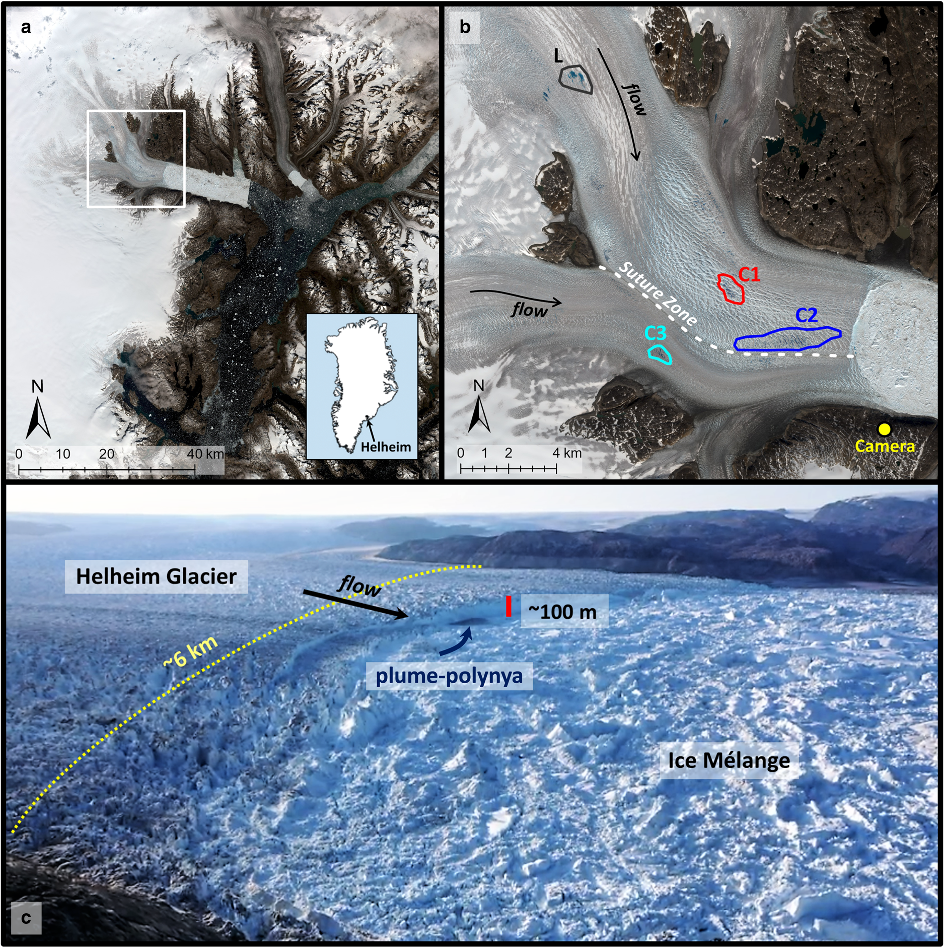
Helheim Glacier's location and setting. (a) True-color Sentinel-2 imagery (10 July 2017) of Helheim Glacier (white box) and surrounding glaciers draining from the Greenland ice sheet into Sermilik Fjord, with the approximate location of Helheim Glacier marked on the inset. (b) Helheim Glacier's terminus region, from the white-box extent in (a). Note the two primary tributaries – flowing as indicated by the black arrows – that meet to form the main glacier trunk where they are separated by a suture zone (dashed white line). Locations of the supraglacial lake (L) and water-filled crevasse areas (C1, C2, and C3) are marked with black, red, blue, and cyan outlines, respectively. The yellow circle represents the location of the time-lapse camera(s). (c) Drone image captured in August 2019, depicting the calving front and ice mélange separated by an ~100 m tall ice cliff. Note the plume-polynya visible at the center of the terminus. Flow is in the direction of the black arrow, and the terminus is ~6 km across.
Types of calving at large tidewater glaciers
Observed calving episodes at tidewater glaciers are diverse, and calving is influenced by both glaciological properties and environmental forcing. Calving behavior depends on a glacier's degree of flotation and state of basal coupling (Walter and others, Reference Walter2010; Olsen and Nettles, Reference Olsen and Nettles2017), which can vary due to ocean tides and local ice thickness changes on daily and even hourly timescales (Hogg and others, Reference Hogg, Shepherd, Gourmelen and Engdahl2016). At large tidewater glaciers in deep fjords, full-thickness calving produces both tabular and non-tabular icebergs (e.g. Joughin and others, Reference Joughin2008; Kehrl and others, Reference Kehrl, Joughin, Shean, Floricioiu and Krieger2017).
Full-thickness tabular icebergs remain floating upright after breaking from floating glacier termini and most commonly form at ice shelves and ice tongues. However, this type of calving may also occur near the grounding line of a tidewater glacier without a tongue if the grounding zone is at or very close to flotation over a sufficient distance to promote longitudinally extensive calving blocks that are dynamically stable in their upright orientation. At lightly grounded tidewater glacier fronts, full-thickness non-tabular icebergs calve due to a buoyancy imbalance when the terminus approaches flotation (e.g. James and others, Reference James, Murray, Selmes, Scharrer and O'Leary2014; Murray and others, Reference Murray2015b; Wagner and others, Reference Wagner, James, Murray and Vella2016). These non-tabular icebergs have height greater than width, and thus they rotate as they calve, usually bottom-out due to basal crevassing, buoyancy forces, and backstress from the mélange (Amundson and others, Reference Amundson2010; James and others, Reference James, Murray, Selmes, Scharrer and O'Leary2014; Murray and others, Reference Murray2015b).
Other types of calving, such as the small subaerial calving amplified by plume-driven undercutting, also occur at large tidewater glaciers. This study, however, focuses on large full-thickness tabular and non-tabular calving episodes which produce clear terminus retreat.
Helheim Glacier
Helheim Glacier (Fig. 1) is Greenland's second-largest glacier by ice discharge (Mankoff and others, Reference Mankoff2019) and the fastest-flowing glacier in East Greenland, with flow speeds reaching over 25 m per day (Rignot and others, Reference Rignot, Braaten, Gogineni, Krabill and McConnell2004; Voytenko and others, Reference Voytenko2015). The glacier terminates in a ~6 km wide subaerial ice cliff that reaches heights up to ~100 m and is lightly grounded in Sermilik Fjord, which is up to 600–900 m deep (Voytenko and others, Reference Voytenko2015; Holland and others, Reference Holland2016). Two primary glacial tributaries meet ~12 km up-glacier from the ice front to form the main trunk, which is divided into northern and southern trunks by a medial moraine-like suture zone, visible as a narrow darker zone parallel to the flow direction (Fig. 1b). The ice at the suture zone was previously at the side of a tributary and is hence likely structurally different from ice elsewhere in the glacier (Holland and others, Reference Holland2016) – possibly because of the presence of impurities or a different strain history – which could influence calving. Terminus depth is greater under the northern trunk (Holland and others, Reference Holland2016), and this trunk also flows at faster velocities (Voytenko and others, Reference Voytenko2015). Approximately 8 km up the northern tributary from the main trunk (~20 km from the ice front) sits a supraglacial lake basin, and both this lake and several crevassed areas regularly fill with surface meltwater during the melt season (Everett and others, Reference Everett2016).
As of 2019, Helheim Glacier had retreated farther and thinned more than at any other time in the observational record (Williams and others, Reference Williams, Gourmelen, Nienow, Bunce and Slater2021). The glacier may retreat rapidly in the future (Williams and others, Reference Williams, Gourmelen, Nienow, Bunce and Slater2021), but it has relatively low global sea-level contribution potential; although it occupies a deep subglacial fjord, the fjord is relatively narrow and the bed rises above sea level to the sides and inland (Nick and others, Reference Nick2013; Felikson and others, Reference Felikson, Catania, Bartholomaus, Morlighem and Noël2021). However, the important processes of meltwater discharge and calving that can currently be observed at the ice-cliff terminus of Helheim Glacier are analogous to processes at other large, lightly grounded outlet glaciers supplied with surface meltwater, now and in the future. Here, observations of plume-polynyas and calving at Helheim Glacier offer the opportunity to study the still-unclear physical mechanisms controlling the relationships between calving frequency and plumes at large tidewater glaciers.
Data and methods
Satellite imagery
To identify plume-polynyas, calving episodes, terminus positions, and supraglacial water storage at Helheim Glacier from 2011 to 2019, we used high-resolution satellite imagery from the Maxar (previously DigitalGlobe) constellation (WorldView-1, -2, and -3; QuickBird; IKONOS; and GeoEye-1), as well as Sentinel-2 and Landsat-8 optical satellite imagery (see Table S1 in the Supplementary material). This time period was chosen due to the density of high-resolution satellite imagery available. Top-of-atmosphere reflectance was calculated for all images. The spatial resolution of Maxar, Sentinel-2, and Landsat-8 imagery was 0.31–3.2, 10, and 15–30 m, respectively (Table S1). The typical time between successive usable Maxar images ranged from a couple of days to several months, while for Landsat-8 and Sentinel-2 the typical range was a couple of days to several weeks. The larger gaps occurred due to cloud cover and dark conditions.
Time-lapse imagery
A single time-lapse camera (StarDot Netcam SC, 5 megapixels), operated by the Cold Regions Research and Engineering Laboratory (CRREL) and positioned just south of Helheim Glacier (66.33° N, 38.174° W) (Fig. 1b), captured images of the terminus from July 2014 through August 2016. This original camera produced 450 images. CRREL then replaced this camera with a dual-camera system of the same camera type. These two cameras both point at the terminus of Helheim Glacier, but one points up-fjord and one down-fjord, enabling visualization of the terminus even as the glacier advances and retreats. Each camera produced 5172 images from the time they were installed in August 2016 through November 2019. The photo interval for all cameras was 3 h, but there were often longer intervals between usable images due to low-light and cloudy/foggy conditions. Nevertheless, in combining the time-lapse imagery with satellite imagery, we were able to increase the temporal resolution of our plume-polynya and calving time series.
Plume-polynya detection
The mélange was intact in all images throughout the study period, so plume-polynyas were visible in satellite and time-lapse imagery as areas of open water surrounded by mélange directly in front of the glacial terminus (Fig. 1). Time-lapse imagery was ideal for determining the existence and duration of plume-polynyas, while satellite imagery supplemented these observations and confirmed plume-polynyas which were very small or obscured by either icebergs in the mélange or the terminus geometry, relative to camera position. We also used satellite imagery to observe plume-polynyas from 2011 to mid-2014, before time-lapse imagery was available, and to map their locations. The lower spatial resolution of Landsat-8 and Sentinel-2 images meant that they were inadequate for observing small plume-polynyas, so a time was marked ‘no plume-polynya’ only if no plume-polynyas were visible in either time-lapse or Maxar imagery.
Calving timing and type
We manually examined successive imagery frame-by-frame to document the timing of calving episodes and iceberg type produced. All clear observations of visible terminus retreat between two consecutive images were attributed to full-thickness calving. Small collapses of the subaerial terminus and purely submarine calving were not observed due to the image resolution. Calving types were distinguished by the iceberg type produced during terminus retreat, as in Kehrl and others (Reference Kehrl, Joughin, Shean, Floricioiu and Krieger2017). Calved tabular icebergs were distinctive due to their rough surface and constant height above the mélange, whereas non-tabular icebergs often broke up and could rarely be identified in the mélange (Fig. 2). Calving episodes were classified into three types: (1) tabular calving, when a tabular iceberg appeared at the terminus and visually accounted for the entire terminus retreat observed; (2) mixed calving, when a tabular iceberg was visible at the terminus but could not visually account for the entire retreat; and (3) non-tabular calving, when terminus retreat occurred without producing a visible tabular iceberg. We refer to calving activity as ‘episodes’ instead of ‘events’ as it is unclear whether observed calving occurred as one event or many events during the time between two successive images (Kehrl and others, Reference Kehrl, Joughin, Shean, Floricioiu and Krieger2017).
Image pairs depicting the difference between non-tabular calving (a, b) and mixed/tabular calving (c, d), as observed in time-lapse imagery. Times are in UTC. Note the terminus-parallel rifting/crevassing before both types of calving (a, c) and the terminus retreat after calving (b, d). A large tabular iceberg is visible in (d), but no distinctive icebergs can be observed in (b). Because the tabular iceberg in (d) does not account for the entire terminus retreat, this is a mixed calving episode.

We used the satellite-derived calving record of Kehrl and others (Reference Kehrl, Joughin, Shean, Floricioiu and Krieger2017) for 2011 through mid-2014 – before the first time-lapse camera was installed. From mid-2014 to mid-2016 (the end of the Kehrl and others record), we validated and supplemented our time-lapse data with their data. The use of both satellite and time-lapse images enabled us to cross-check observations from different perspectives, which was especially critical for processes occurring toward the far north end of the terminus where time-lapse image quality was lower.
Terminus position
Terminus position was measured from satellite imagery to provide context into advance and retreat patterns of Helheim Glacier. We manually digitized 388 terminus positions from March 2011 to December 2019, then calculated the area within a standard open-ended box behind each digitized terminus and divided this by the width. This method, which generates width-averaged measures of changes in terminus position, was established by Schild and Hamilton (Reference Schild and Hamilton2013) based on Moon and Joughin (Reference Moon and Joughin2008) and Howat and others (Reference Howat, Joughin, Fahnestock, Smith and Scambos2008).
Supraglacial meltwater
To compare the plume-polynya time series with supraglacial meltwater storage and release, we investigated the timing of water pooling on the surface of Helheim Glacier. In addition to the supraglacial lake (L) described by Everett and others (Reference Everett2016), we observed three areas in the highly crevassed downglacier region that regularly filled with supraglacial meltwater each summer (Fig. 3).
Surface meltwater pooling visualized in true-color QuickBird imagery captured on 24 August 2011 (© 2011 Maxar Technologies, Inc.). (a) The regions of interest – L, C1, C2, and C3 – are marked and labeled in black, red, blue, and cyan, respectively. Pan-sharpened true-color Maxar imagery reveals morphological details of the supraglacial lake (b) and meltwater-filled crevasse areas C1 (c), C2 (d), and C3 (e). In this particular image, all areas contain pools of supraglacial water, yet none are filled to the maximum meltwater capacity observed in other images.

The surface area of meltwater is a proxy for water volume stored on the glacier surface. Surface area is unlikely to vary linearly with water volume in deep, narrow crevasses and would not be appropriate for estimating water budgets, but it is a suitable measurable parameter for our focus on the timing of filling and draining (e.g. Danielson and Sharp, Reference Danielson and Sharp2013). To calculate the area of water in each study area, we relied on the spectral differences between supraglacial water and bare glacial ice in satellite imagery (Fig. S1). To increase the spatial resolution of multispectral Landsat-8 images while preserving the spectral characteristics, multispectral bands were pan-sharpened to 15 m resolution using the Gram–Schmidt spectral-sharpening algorithm (Laben and Brower, Reference Laben and Brower2000). Then, the normalized difference water index for ice (NDWIice) was calculated (Fig. S1b). NDWIice, developed by Yang and Smith (Reference Yang and Smith2013), is a normalized ratio of the red and blue bands:

where BLUE and RED are the spectral reflectivities of these wavelengths measured in the blue and red bands of the imagery.
NDWIice was calculated for cloud-free satellite imagery. Both Sentinel-2 and pan-sharpened Landsat-8 imagery clearly showed the timing of surface water storage with greater temporal resolution than Maxar imagery. Sentinel-2 imagery was ideal because it required less processing than Landsat-8 (no pan-sharpening). We therefore utilized Sentinel-2 when imagery was available (2016–19), Landsat-8 imagery before that when available (2013–15), and Maxar imagery before either Sentinel-2 or Landsat-8 were launched. One type of satellite imagery was used for each time interval.
We determined NDWIice thresholds to classify images into water and water-free regions (Fig. S1c). Both shadows and slush on the glacier surface complicated this process, as shadowed ice and slush have high NDWIice values similar to those of water. We decided to use two different thresholds: one more liberal threshold for the lake to identify as many water pixels as possible; and one narrower threshold for the crevasse regions, which were often more shadowed due to greater topographic relief. Different thresholds were also used for Sentinel-2, Landsat-8, and Maxar imagery. These threshold choices were made by comparing the NDWIice values of pixels manually identified as water versus ice in the areas of interest, to produce water classification results that matched those obtained by manually identifying the water areas. NDWIice thresholds for L (C1, C2, and C3) were 0.11 (0.21), 0.08 (0.11), and 0.22 (0.35) for Sentinel-2, Landsat-8, and Maxar, respectively.
After applying these thresholds, the rasters were clipped to the shapefile areas of interest. These areas remained consistent throughout the study period and across different satellite imagery products. The number of ‘water’ pixels in each area was multiplied by pixel area to calculate the surface area of water present in each area through time.
Subglacial hydraulic potential
To establish where water was routed subglacially and compare this with plume-polynya and surface water locations, we combined bed and surface topography into a numerical model for subglacial hydraulic potential. Gradients in subglacial hydraulic potential govern the flow routing of basal water (Shreve, Reference Shreve1972). We calculated subglacial hydraulic potential (Φ) as:

where ρ i and ρ w are the density of ice (917 kg m−3) and water (1000 kg m−3), respectively; g is the acceleration due to gravity (9.18 m s−2); h and z are the ice surface and bed elevations, respectively; and k is the cryostatic pressure factor (as in Everett and others (Reference Everett2016) and How and others (Reference How2017)). k is a fraction of ice-overburden pressure and is often set to 1, which assumes the catchment is at overburden pressure.
For the ice surface and bed elevations, we used the 150 m spatial resolution IceBridge BedMachine Greenland Version 3 surface and bed digital elevation models (DEMs) (Morlighem and others, Reference Morlighem2017). We calculated subglacial hydraulic potential over a range of k values from 0.9 to 1.2 to represent a range of overburden fractions likely present at the glacier bed over time and space (Everett and others, Reference Everett2016). Sinks in the hydropotential surface rasters were filled, then flow direction and flow accumulation (accumulated weight of upslope cells that flow into each downslope cell) were calculated with the D-infinity flow method (Tarboton, Reference Tarboton1997). We then passed a 3 × 3 low-pass filter over the flow accumulation data to smooth flow-routing lines.
Observations and results
The 2011–19 time series of plume-polynya visibility, calving, terminus position, and supraglacial water area are displayed in Figure 4. To better visualize the details of these data, we also display this time series in smaller intervals: 2011–13 (Fig. 5), 2014–16 (Fig. 6), 2017–19 (Fig. 7), and 2019 (Fig. 8). These figures all depict the timing of plume-polynya appearance at the terminus of Helheim Glacier (Figs 4a–8a) and how this relates to the timing and type of calving, relative terminus position (Figs 4b–8b), and the timing of surface meltwater pooling and drainage (Figs 4c–8c).
Time series of observations from Helheim Glacier, 2011 through 2019. (a) Calving type, top, with plume-polynya presence, bottom, represented as color bars. (b) Mean terminus position relative to the most advanced position observed in early 2011. (c) Surface area of supraglacial water in L, C1, C2, and C3 (note the offset axis). Color bars in (b) and (c) mark calving type and plume-polynya presence.

Time series of observations from Helheim Glacier, 2011 through 2013: (a) calving type, top, with plume-polynya presence, bottom; (b) mean terminus position; and (c) surface area of supraglacial water in L, C1, C2, and C3. Color bars in (b) and (c) mark calving type and plume-polynya presence.

Time series of observations from Helheim Glacier, 2014 through 2016: (a) calving type, top, with plume-polynya presence, bottom; (b) mean terminus position; and (c) surface area of supraglacial water in L, C1, C2, and C3. Color bars in (b) and (c) mark calving type and plume-polynya presence.

Time series of observations from Helheim Glacier, 2017 through 2019: (a) calving type, top, with plume-polynya presence, bottom; (b) mean terminus position; and (c) surface area of supraglacial water in L, C1, C2, and C3. Color bars in (b) and (c) mark calving type and plume-polynya presence.

Time series of observations from Helheim Glacier in 2019: (a) calving type, top, with plume-polynya presence, bottom; (b) mean terminus position; and (c) surface area of supraglacial water in L, C1, C2, and C3. Color bars in (b) and (c) mark calving type and plume-polynya presence.

Plume-polynya locations and timing
Plume-polynyas consistently surfaced near the center of the terminus, even as the terminus advanced and retreated several kilometers. Notably, most plume-polynyas were ~1.2 km northeast of the suture zone along the terminus (Fig. 9), similar to plume positions determined by Everett and others (Reference Everett, Murray, Selmes, Holland and Reeve2021). However, two plume-polynyas (12 September 2011 and 29 July 2014) were only ~300 m from the suture zone, ~900 m south-southwest of the others (consistent with the location of the plume observed by Everett and others (Reference Everett, Murray, Selmes, Holland and Reeve2021) in late July 2014). In addition, all the plume-polynyas visible in 2019 were ~200 m south-southwest of the previous line of plume-polynyas, closer to the suture zone (Fig. 9).
Locations and visualizations of plumes surfacing as plume-polynyas at the terminus of Helheim Glacier. (a) Colored circles depict locations of all 21 plume-polynyas observed in satellite imagery from 2011 to 2019, and lines represent the corresponding terminus positions. Background panchromatic WorldView-1 imagery was acquired on 24 June 2012 (© 2012 Maxar Technologies, Inc.). Panchromatic imagery shows detailed morphology of plume-polynyas on (b) 16 April 2017 (WorldView-2); (c) 2 July 2014 (WorldView-2); and (d) 24 June 2012 (WorldView-1), © 2017, 2014, and 2012 Maxar Technologies, Inc.

Although the satellite imagery often provided just a few snapshots of the surfacing plumes, the time-lapse imagery allowed observations of plume-polynya changes through time and the duration of their persistence. We observed 24 plume-polynyas in total, 11 of which were in 2019 (Table 1). No plume-polynyas were detected in 2013 or 2018, though for 2013 this was due to poor data coverage (see Everett and others (Reference Everett, Murray, Selmes, Holland and Reeve2021) for information on 2013 plumes). Plume-polynya duration ranged from 1 to 29 d. Although the plumes primarily surfaced during the summer from late-June through September, eight plume-polynyas were visible at other times (mid-April, May, early-June, and early-October) (Table 1). Where plume-polynya data overlap, our plume record is completely consistent with that of Everett and others (Reference Everett, Murray, Selmes, Holland and Reeve2021).
Dates of plume-polynya appearance observed from satellite and time-lapse imagery, duration of plume-polynya visibility from time-lapse imagery, and dates of the next calving episode after plume-polynya disappearance

Superscripts M, L, and S indicate Maxar, Landsat-8, and Sentinel-2 satellite imagery, respectively.
Calving
Of 200 full-thickness calving episodes classified from 2011 through 2019, 169 (84.5%) were non-tabular, 22 (11%) were mixed, and 9 (4.5%) were tabular (Figs 4–8). These data are, however, limited by few winter observations. Tabular calving generally occurred during winter or spring, or when the terminus was in an advanced state (as in mid-2011). Mixed calving episodes occurred throughout the year, and in 2016 and 2018 this type of calving was relatively more common. Non-tabular calving episodes, although more frequent in the summer, also occurred through all seasons.
Non-tabular calving often occurred in a succession of several distinct events along different areas of the terminus, consistent with the observations of Holland and others (Reference Holland2016). Calving sequences were distinguished by separate retreat along the northern and southern termini with a discontinuity near the suture zone. In some cases, icebergs calved from seemingly disconnected areas of the terminus at the same time (e.g. Figs 2a, b). Distinctive terminus-parallel rifting (consistent with ‘flexion zones’ in Murray and others, Reference Murray2015b) often preceded calving (e.g. Figs 2a, c). In mixed calving episodes, observed tabular icebergs were typically small and broke off the southern or northern terminus while non-tabular calving accomplished the primary terminus retreat. Nevertheless, we also observed several examples of distinctive large tabular icebergs in the mélange – sometimes calved during mixed episodes (e.g. Fig. 2d) and sometimes during purely tabular episodes.
Plume-polynyas and calving
Comparisons between the timing and characteristics of plume-polynyas and calving episodes reveal a relationship between the two processes. Although non-tabular calving occurred both before and immediately after plume-polynya appearance, no calving episodes large enough to cause visible terminus retreat occurred while a plume-polynya was visible, with only one exception (Figs 4a–8a). This one exception was on 16 April 2017, when a tabular iceberg calved from the far-northern terminus while a plume-polynya was visible at the center of the terminus (Fig. 10). Both the tabular iceberg and the plume-polynya are visible in the same satellite images, so we are sure that these events occurred concurrently but were separated spatially.
Satellite imagery of the terminus of Helheim Glacier from 16 April 2017 depicting tabular calving at the northern terminus while a plume-polynya is observed at the center of the terminus. (a) True-color Landsat-8 image, with black box indicating the extent of (b). (b) True-color WorldView-2 image (© 2017 Maxar Technologies, Inc.). Note the plume-polynya in the cyan dashed circle and tabular iceberg to the north.

Crevasses and surface slumping typically appeared at the glacial terminus directly south of the plume-polynyas (e.g. Figs 11a, b). This apparent slumping could be failure along a slope from the surface to the waterline, as described by Parizek and others (Reference Parizek2019). Interestingly, non-tabular calving episodes often coincided with (within the time between successive images) or followed each plume-polynya's disappearance, accompanied by terminus retreat either directly south of where the plume-polynya had been (e.g. Fig. 11c) or across most of the terminus. Of the 18 plume-polynyas observed in the 2015–19 time-lapse imagery, 11 were followed by calving on either the same day as their disappearance or the next day (Table 1). Calving occurred 2–3 d after two of these plume-polynyas disappeared and over a week after five other plume-polynyas disappeared.
Consecutive time-lapse images from 18 July 2017, captured at 06:00 (a), 09:00 (b), and 12:00 (c). Times are in UTC. Images depict a surfacing meltwater plume (cyan dashed oval) with crevassing (red dashed line) to the south (a), followed by the plume's disappearance (b), then terminus retreat due to non-tabular calving in the south (c).

Terminus advance and retreat
The terminus of Helheim Glacier retreated and re-advanced seasonally. This annual cycle of summer retreats and winter advances consisted of terminus position fluctuations of up to ~3–3.5 km (Fig. 4b). Superimposed on this was an overall trend of terminus retreat. The most advanced terminus position measured was on 10 March 2011 (defined as zero), while the most retreated position was on 8 September 2019, when the terminus was >5.6 km behind the 10 March 2011 position (Fig. 4b). Much of this retreat occurred during the 2017 and 2019 summers, when the terminus retreated ~1.5 km beyond any previously observed positions (Figs 4b, 7b).
Supraglacial meltwater storage and release
The maximum surface area of water in L varied each year, ranging from 0.20 km2 in 2018 to 0.57 km2 in 2015 (Figs 4c–8c). The peak in L area typically occurred in June or July, and in 2015, 2016, 2017, and 2019 a second distinctive peak in L water area occurred in July, August, or September. The water area in C1, C2, and C3 ranged from 0–0.31, 0–0.55, and 0–0.15 km2, respectively. Areas C1, C2, and C3 filled and drained roughly synchronously, yet in some years C3 peaked before C1 and C2. Typically, filling and draining of these downglacier crevassed regions occurred soon after or during the first drainage of L. The clearest deviation from this pattern was in 2018 when there was no distinctive peak in L area; L instead followed a similar filling and draining sequence as the crevasse areas (Fig. 7c). We also did not observe a difference in timing of L drainage compared to C1, C2, and C3 drainage from 2011 to 2013 (Fig. 5c), but this was perhaps due to insufficient data coverage, as Everett and others (Reference Everett2016) did observe L drainage before filling and draining of downglacier crevasse regions in these years.
When plume-polynyas appeared, it was generally after drainage of L and while C1, C2, and C3 crevasses contained measurable quantities of water (Figs 4c–8c). In 2018, when L area did not peak as in other years, no plume surfaced at the terminus of Helheim Glacier. Nevertheless, C1, C2, and C3 filled with water during summer 2018. In 2017, however, a plume-polynya appeared in April before surface water was visible in L or within any crevasse areas. Similarly, the first plume-polynya of 2019 appeared in early May while meltwater was just starting to collect on the surface.
Subglacial water flow
The subglacial hydraulic potential model identified areas of high flow accumulation as strong meltwater routing locations. Subglacial flow accumulation maps calculated with different k values (Fig. 12) show that the modeled subglacial flow was routed to one, two, or three prominent meltwater discharge locations, depending on the terminus position. Plume-polynya locations aligned well with the central discharge location (Fig. 12). Additionally, supraglacial meltwater pooling areas L, C1, C2, and C3 all aligned with areas where different modeled subglacial flow routing configurations converged at hydropotential lows, which represented locations of the main subglacial channels in the model.
Shaded subglacial flow routes determined from flow accumulation calculations over hydraulic potential surfaces. Different values of k, representing different overburden fractions, produced different flow pathways – shaded in blue (k = 1.00), purple (k = 1.10), and green (k = 1.14). Contours of hydraulic potential (k = 1.00) with spacing intervals of 1 MPa (major) and 0.25 MPa (minor) overlie the flow paths. Supraglacial lake and water-filled crevasse areas are marked, and cyan circles at the terminus show plume-polynya locations, from Figure 9. The main map (a) depicts the three different flow configurations together, while they are depicted separately in (b), (c), and (d). The background is a true-color Sentinel-2 image from 7 May 2016. Slight differences in flow paths from those reported by Everett and others (Reference Everett2016) are likely due to differences in BedMachine versions (v3 here versus v2 in Everett and others (Reference Everett2016)).

At lower values of k (<0.99), hydraulic potential gradients were steeper, and flow was mostly confined to within bed troughs, with no strong flow between C1 and C2. When k was just below 1 (~0.99), flow redirected to cross between two bed troughs from near-C1 to mid-C2. Subglacial flow accumulation routing over a hydraulic potential surface calculated with k = 1.00 (Fig. 12b) was nearly identical to that when k = 0.99. As k increased above 1 (Figs 12b, c), hydraulic potential gradients decreased, and flow redirected more with smaller variations in k.
Discussion
Plume-polynya and calving interactions
Except for the one spatially separated observation of tabular calving during plume-polynya presence (Fig. 10), no full-thickness calving (tabular, non-tabular, or mixed) occurred while a plume-polynya was visible. These results suggest that either full-thickness calving suppressed the plume-polynyas, or discharging plumes suppressed full-thickness calving (Bunce and others, Reference Bunce, Nienow, Sole, Cowton and Davison2021; Everett and others, Reference Everett, Murray, Selmes, Holland and Reeve2021). Perhaps calving disturbed channel and plume-polynya formation, or the conditions which created plume-polynyas inhibited calving.
Buoyant plumes that melt the submarine terminus while rising from the base of the glacier could reduce the buoyancy of the terminus and hinder calving, as proposed by Everett and others (Reference Everett, Murray, Selmes, Holland and Reeve2021). Alternatively, calving could suppress plumes if basal crevasses, which are important in full-thickness calving initiation (James and others, Reference James, Murray, Selmes, Scharrer and O'Leary2014; Murray and others, Reference Murray2015b), interrupted the plume subglacially. Even if calving did not disrupt the plume at depth, newly formed icebergs and bergy bits in the fjord could obscure the plume-polynya feature observed at the surface.
While plume-driven submarine melting and the consequent reduction in terminus buoyancy may play a role in the observed relationship between plume-polynya appearance and full-thickness calving, we question whether the localized melt at the plume location would completely interrupt all full-thickness calving across the entire terminus. Over the nine years of observations in this study, we observed only one example of full-thickness calving during plume-polynya presence, and in this case the calved iceberg was removed spatially from the plume-polynya (Fig. 10). The rarity of full-thickness calving during plume-polynya presence suggests that calving and/or plume-polynya processes usually suppress each other across the whole terminus. Nevertheless, the one observation of concurrent tabular calving and plume-polynya presence also indicates that there are, at times, exceptions to this pattern.
Newly formed icebergs and bergy bits may sometimes obscure plume-polynyas, but this also cannot fully explain the observed relationship between calving and plume-polynyas. In 2011–18, every time plume-polynya disappearance was associated with a calving episode, there was always at least one image frame between plume-polynya disappearance and calving. This indicates that the plume-polynyas disappeared before calving occurred; hence, ice debris from calving could not have been the only reason for plume-polynya disappearance. In 2019, however, it was often unclear whether plume-polynya disappearance or calving occurred first, as one time-lapse photo showed a polynya, then the next depicted a retreated terminus (at least 3 h later).
Plume-polynya disruption by basal crevassing remains a reasonable mechanism to explain why all plume-polynyas and full-thickness calving episodes were separated either by time or space. Basal crevasses form close to the grounding line if basal water is pressurized, ice is subjected to tensile stress, and the glacial front is out of buoyant equilibrium (van der Veen, Reference van der Veen1998). When close to the calving margin, basal crevasses allow the terminus to lift and rotate backward (James and others, Reference James, Murray, Selmes, Scharrer and O'Leary2014; Murray and others, Reference Murray2015b). Basal crevasses associated with buoyancy-driven full-thickness calving would interrupt a plume discharging at the base of the glacier when they intersected the channel or plume location. Still, this mechanism does not fully explain why there are times when the plume does reach the fjord surface, forms a plume-polynya, and remains visible for up to 29 d (Table 1) without being interrupted by calving. There is therefore likely another way in which the conditions leading to plume-polynyas inhibit full-thickness calving. We propose a mechanism to explain the ceased calving activity during plume-polynya appearance that involves the subglacial water pressure and drainage configuration, along with basal crevasses.
Subglacial water flows down a potential gradient, so basal water must be at a higher pressure than the fjord water column to discharge to the fjord (Walker and others, Reference Walker2013). In grounded regions, where the ice-overburden pressure is greater than the water column pressure, the subglacial water pressure can be less than the ice-overburden pressure and still discharge into the fjord. This configuration represents the channelized low-pressure basal water system from which plumes discharge. When the ice-overburden pressure drops close to the water column pressure while approaching flotation, the subglacial water pressure must rise until water spreads into the linked-cavity basal system, thickening and expanding that system until it locally floats the glacier. In this configuration, subglacial discharge will be distributed along the terminus and will no longer enter the fjord as a concentrated plume.
Consequently, we hypothesize that plume-polynyas only appear at the terminus of Helheim Glacier when the glacier front is grounded. A completely grounded glacial front will suppress full-thickness calving if basal crevasses are unable to form. Conversely, whenever full-thickness calving occurs, this indicates that the terminus of Helheim Glacier is at or close to flotation and that basal crevassing can occur. We suggest that our time series of plume-polynya appearance and calving occurrence therefore represent proxies for the grounding state of Helheim Glacier, although our ability to constrain transient flotation near and across the grounding line is limited by the temporal resolution of the data.
From terminus-wide observations, plume-polynyas and calving were generally separated not only in time but also in space, suggesting that plume-polynya appearance usually indicated grounding across the entire terminus of Helheim. However, there must also have been times when basal coupling conditions varied across the glacial front, as observed in Figure 10. The northern terminus, which sits above the deepest part of the bed, must be capable of going to flotation even when a plume is discharging from a grounded central terminus.
We acknowledge the alternative hypothesis that a discharging plume could continue rising from a subglacial channel to appear as a plume-polynya even as the terminus gradually approached flotation, only stopping when interrupted by a basal crevasse. Plume-polynyas do, in fact, exist at ice-shelf edges in Antarctica – fed by channels under the shelves that originate at the grounding line (Alley and others, Reference Alley, Scambos, Siegfried and Fricker2016; Alley and others, Reference Alley, Scambos, Alley and Holschuh2019a). Additionally, we note that the stability of the subglacial channel's position inferred from consistent plume-polynya locations suggests that the channel itself likely remained intact through calving episodes. Large openings have also been found where plumes emerge from other glacier termini (Fried and others, Reference Fried2015; Rignot and others, Reference Rignot, Fenty, Xu, Cai and Kemp2015). Perhaps a plume could carve into the floating glacial front enough to remain constrained and continue surfacing as a polynya; however, this process would take time. At Helheim Glacier this is likely limited by the rapid calving rate and limited size of the floating extension.
Supraglacial, englacial and subglacial water
Supraglacial lake drainage can transport a large quantity of meltwater to the subglacial environment. Lake L's basin can contain a water volume of up to 107 m3, and the lake has been observed to drain down a moulin southwest of the basin (Everett and others, Reference Everett2016). We found that drainage of L was usually followed by filling and draining of downglacier crevassed regions, consistent with the findings of Everett and others (Reference Everett2016). This is different from the typical up-glacier progression elsewhere in Greenland (e.g. Danielson and Sharp, Reference Danielson and Sharp2013; How and others, Reference How2017), demonstrating that subglacial hydrologic networks with different meltwater input locations have different seasonal evolution characteristics.
Lake drainage early in the melt season would initially overcome the capacity of the subglacial drainage system and raise basal water pressure (Das and others, Reference Das2008). Then, the subglacial network could reorganize into a higher-capacity low-pressure system of R-channels (Röthlisberger, Reference Röthlisberger1972). In most years, plume-polynyas appeared after filling and drainage of L, suggesting that lake drainage may have played a role in converting the basal water system into the channelized configuration or enlarging a residual channel sufficiently to produce a plume-polynya. Notably, 2018 was the only year during which there was no distinctive peak in L and also the only year covered by time-lapse imagery in which we did not observe any plume-polynyas. However, plume-polynyas appeared before observed filling and drainage of L in both 2017 and 2019, so lake drainage must not always be required to create a channelized system.
Plume-polynyas were consistently located near the central discharge location in the subglacial flow accumulation model, in between two bed topographic lows (Fig. 12). This supports the idea that the plume-polynyas were sourced from ice-incised R-channels (Röthlisberger, Reference Röthlisberger1972) rather than bedrock-incised N-channels (Cuffey and Paterson, Reference Cuffey and Paterson2010). However, higher-resolution bed mapping would be needed to rule-out the existence of N-channels. Slight subglacial R-channel reconfigurations could explain the location of the plume-polynyas observed on 12 September 2011 and 29 July 2014, south of the primary line of plume-polynyas, as well as the smaller difference in 2019 plume-polynya locations. There is likely substantial variability in k across Helheim Glacier both spatially and temporally, and switches in flow routing can occur rapidly, especially at higher values of k expected with higher subglacial pressure.
Because the plume-polynya location at the central terminus reflects an established R-channel source, plume-polynyas must have appeared only when the subglacial hydrologic system was in a low-pressure channelized configuration. The timing of plume-polynya appearance correlated with filling or water presence in the surface crevasse areas (C1, C2, and C3), so when crevasses filled with water during plume-polynya presence, they must have filled during an overall state of low subglacial pressure.
Notably, C1, C2, and C3 were all located where subglacial water encountered adverse bed slopes while flowing out of overdeepenings (Fig. 13). Water pressure increases and flow paths can split when basal water flows out of a bed overdeepening (Alley and others, Reference Alley, Cuffey and Zoet2019b; Vore and others, Reference Vore, Bartholomaus, Winberry, Walter and Amundson2019), so these locations should have had locally elevated basal pressure (and k values), favoring subglacial flow path branching. Furthermore, Shreve's (Reference Shreve1972) model for subglacial hydraulic potential breaks down at steep adverse bed slopes; here the pressure-melting point increases, more viscous energy is needed to warm the water, and less energy is available to maintain the subglacial conduit (Hooke and Pohjola, Reference Hooke and Pohjola1994). Conduits in this situation can freeze closed, forcing basal water to flow around overdeepenings and some to enter the englacial system (Hooke and Pohjola, Reference Hooke and Pohjola1994). The ratios of bed to surface slopes out of the overdeepenings beneath C1, C2, and C3 range from −2.5 to −40 (calculated from BedMachine Greenland v3 bed and surface DEMs (Morlighem and others, Reference Morlighem2017)) and are therefore all of greater magnitude than the supercooling threshold of −1.6. Where the local slope ratio is of greater magnitude than this threshold, supercooling of subglacial conduits as described above can occur (Röthlisberger and Lang, Reference Röthlisberger, Lang, Gurnell and Clark1987; Alley and others, Reference Alley, Lawson, Larson, Evenson and Baker2003; Werder, Reference Werder2016). Furthermore, for ratios of bed to surface slope of greater magnitude than ~−11, subglacial water flow can reverse (e.g. Alley and others, Reference Alley, Lawson, Evenson, Strasser and Larson1998).
Supraglacial water areas overlain on bed elevation from BedMachine Greenland v3 (Morlighem and others, Reference Morlighem2017). Cyan circles at the terminus mark plume locations from Figure 9, lake and water-filled crevasse areas are indicated, and the gray and white dashed lines delineate the 24 June 2012 and 8 September 2019 terminus positions, respectively. Background is a true-color Sentinel-2 image from 10 July 2017.

The spectral characteristics of the water in C1, C2, and C3 indicate that it was not turbid water sourced from the subglacial environment and must have been either surface or englacial water (Everett and others, Reference Everett2016). Connections between basal and surface water must not be efficient enough to bring turbid water to the surface, suggesting a dense englacial hydrologic network (Vaňková and others, Reference Vaňková2018). Elevated englacial flow over bed overdeepenings (Hooke and Pohjola, Reference Hooke and Pohjola1994) and locally increased basal pressure therefore could have either driven englacial water into overlying surface crevasses or prevented surface meltwater from draining in the C1, C2, and C3 areas.
In the summers of 2017 and 2019, the terminus of Helheim Glacier retreated to the downglacier edge of C2 (Figs 9, 13). These summers also corresponded with the the most frequent occurrences of plume-polynyas (Figs 4, 7), which appeared in front of C2. This indicates that C2 and the englacial hydrologic system there could be connected to the subglacial hydrologic network which produced the plume.
We note that, despite the connection between lake L and discharge locations, lake drainage cannot be the only source of water contributing to discharging plumes; plume-polynyas appeared before lake drainage in 2017 and 2019, and not all lake drainages were followed by plume-polynyas. Firn aquifers up-glacier of our study area drain through crevasses to the bed, supplying Helheim Glacier with water outside of the typical melt season (Poinar and others, Reference Poinar2017), and the channel feeding the plume may therefore exist even through winter, fed by the firn aquifer water (Poinar and others, Reference Poinar, Dow and Andrews2019). Other water sources at Helheim Glacier include surface melt over the entire catchment and water stored in the subglacial system. Further research should compare the water volumes and seasonal volume changes of these reservoirs, as well of the timing of meltwater discharge, to better constrain the sources of plume water and controls on plume discharge.
Limitations of plume-polynya observations
We recognize that there are several other possible reasons for plume-polynya disappearance that are not fully constrained in this study. Our conservative record of plume existence from surface observations of plume-polynyas does not acknowledge the times when a plume enters the fjord at depth without rising through the mélange. Both the existence of a discharging plume and whether it reaches the surface before reaching neutral buoyancy are subject to the organization of the subglacial water system, meltwater discharge volume and rate, fjord stratification, and mélange rigidity (Carroll and others, Reference Carroll2015, Reference Carroll2016; Slater and others, Reference Slater, Nienow, Cowton, Goldberg and Sole2015; De Andrés and others, Reference De Andrés2020; Everett and others, Reference Everett, Murray, Selmes, Holland and Reeve2021) – variables that are unconstrained in the current study. Additionally, the plume-polynya could disappear if terminus advance down a slope into deeper water caused the plume to reach neutral buoyancy below the waterline. Smaller plumes without surface expression also could have entered the fjord at other discharge locations; these would have been unobservable in optical satellite imagery.
Conclusions
Analyses of satellite and time-lapse imagery of Helheim Glacier from 2011 to 2019 reveal relationships between subglacial discharge plumes, full-thickness calving, and meltwater drainage governed by evolving subglacial hydrology and basal coupling. Coupling between the glacier and the bed is itself complex, depending on ice thickness, fjord geometry and terminus position, subglacial hydrologic drainage configuration, and tidal phase (see the Supplementary material). As Helheim Glacier advances and retreats over basal troughs and overdeepenings, spatial and temporal variability in the degree of flotation drive differences in calving and subglacial hydrology. We summarize our observations and interpretations of the spatial and temporal connections between glacial hydrology and calving at Helheim Glacier below.
The basal water system evolves seasonally, forming an established R-channel network when supplied with enough water. A supraglacial lake fills and drains during summers, releasing meltwater into the subglacial environment and possibly playing a role in converting the basal water system into a channelized network. Where subglacial flow paths split and water flows over overdeepenings at locally higher pressure, basal water enters the englacial network. Higher basal pressure and increased englacial water at these locations prevent meltwater from draining down overlying crevasses, and englacial water may also enter crevasses. When a subglacial channel intersects with the grounded central terminus of Helheim Glacier, it discharges buoyant freshwater, which rises as a plume. We observe plume-polynyas, the surface expressions of plumes, only when they rise all the way to the fjord surface and through the mélange.
Whenever these plume-polynyas are visible, full-thickness calving either stops completely or is spatially removed from the plume-polynya. We hypothesize that this is because the low-pressure channelized subglacial hydrologic system and grounded terminus which support plume-polynya existence suppress basal crevasses and full-thickness calving. When the terminus approaches flotation, however, subglacial water pressure must rise until discharging water spreads out along the terminus. These high-pressure subglacial conditions should both result in plume-polynya disappearance and promote basal crevassing and full-thickness calving.
The processes observed at Helheim Glacier should also exist at other marine-terminating glaciers, but the ways in which meltwater discharge and calving interact surely vary with fjord geometries. Other glaciers that are supplied with surface melt, that terminate in deep fjords, that shift between grounded and floating, and that have tall ice-cliff calving faces likely would show similar behavior to that observed here. Further research on the feedbacks between glacier hydrology, calving, and other dynamic terminus processes should reveal additional important controls on glacier behavior in a warming world.
Supplementary material
The supplementary material for this article can be found at https://doi.org/10.1017/jog.2021.141.
Acknowledgements
The research by S.M.M. was supported by an NSF Graduate Research Fellowship (award number 1745025). The Heising-Simons Foundation provided financial support for Greenland fieldwork and the time-lapse cameras (award numbers 2017-316 and 2018-0769). NSF-NERC award 1738934 also supported this research. Maxar satellite imagery and geospatial support (including initial image processing, orthorectification with ArcticDEM 2-m data, and projection to EPSG 3413 NSIDC Sea Ice Polar Stereographic North) were generously provided by Cathleen Torres Parisian of the Polar Geospatial Center, under NSF-OPP awards 1043681 and 1559691. The authors offer special thanks to Laura Kehrl and Ian Joughin for granting access to their calving data, and to Alistair Everett and two anonymous reviewers, whose thoughtful comments greatly improved this manuscript. We are also immensely grateful to Nouf Waleed Alsaad, Luke Trusel, and Christelle Wauthier for their insight; the Penn State Ice and Climate Exploration research team; and the Penn State Geosciences Department. All data reported in this manuscript are available upon request.


 Open access