


1. Introduction
This research investigates whether the transmission of monetary policy is conditioned by varying levels of household debt. We address this question by analyzing the aggregate effects of monetary policy across the world’s seven largest economies and three highly indebted economies, Australia, Sweden, and Norway, within a unified empirical framework. By quantifying these effects across distinct debt regimes, we contribute to the expanding literature on private debt dynamics, specifically addressing a critical gap: the reliance of existing studies on exogenous regime identification.
Although several theoretical explanations have been proposed to explain the effects of household debt on monetary policy, the empirical literature remains divided. Kim and Lim (Reference Kim and Lim2020), using an interacted Panel VAR model, finds that monetary policy is more powerful during periods of high household debt. On the contrary, Alpanda and Zubairy (Reference Alpanda and Zubairy2019) and Beraja et al. (Reference Beraja, Fuster, Hurst and Vavra2019) find that policy effects are diminished when households are highly indebted. This lack of consensus may be attributed to the difficulty of defining debt regimes; unlike GDP fluctuations, household debt is governed by financial cycles that operate on longer horizons than standard business cycles (Terrones et al. Reference Terrones, Claessens and Kose2011). Existing research often relies on exogenous trend deviations to identify these regimes, which may fail to capture true inflection points. We address this by employing an endogenous identification strategy within an STVAR framework. Within this framework, we specifically focus on the impact of expansionary monetary policy, namely, interest rate reductions, to determine how debt levels condition the effectiveness of a stimulus.
Our focus on interest rate reductions is motivated by the theoretical expectation that expansionary policy provides a disproportionate stimulus in leveraged economies. This mechanism, however, remains an open debate centered on the tension between the cash-flow channel and collateral constraints. On one hand, highly indebted households often exhibit a higher marginal propensity to consume (MPC), potentially amplifying the effects of rate cuts through the relaxation of liquidity constraints (Mian et al. Reference Mian, Sufi and Verner2017; Cloyne et al. Reference Cloyne, Ferreira and Surico2020; Blundell et al. Reference Blundell, Pistaferri and Preston2008). Conversely, the effectiveness of such stimulus may be undermined by fixed-rate mortgage structures, the financial accelerator effect, or borrowing capacity constraints that force deleveraging even as rates fall (Alpanda and Zubairy, Reference Alpanda and Zubairy2019; Bernanke et al. Reference Bernanke, Gertler and Gilchrist1999; Beraja et al. Reference Beraja, Fuster, Hurst and Vavra2019). Given these competing wealth and income effects, the net impact of debt on policy potency remains a critical empirical question.
Does household debt affect the transmission mechanism of monetary policy? We address this question using a Smooth Transition Vector Autoregression (STVAR) model. Our approach identifies debt regimes endogenously using a logarithmic transition function, allowing us to quantify the impact of a negative monetary policy shock during periods of high and low household debt without relying on exogenous trend deviations. By employing a Bayesian estimation, we distinguish between the immediate output response and the medium-term persistence of the shock. In contrast to studies using loan-level data from a single country (Beraja et al. Reference Beraja, Fuster, Hurst and Vavra2019), our use of aggregate macroeconomic data across ten distinct economies allows for a broader assessment of these non-linearities in diverse institutional settings.
Our choice of the empirical model is based on its ability to identify debt regimes endogenously, a feature crucial given the lack of formal criteria for defining debt thresholds. Unlike Kim and Lim (Reference Kim and Lim2020) and Alpanda and Zubairy (Reference Alpanda and Zubairy2019), who identify debt states based on positive deviations of the debt-to-GDP ratio from a Hodrick-Prescott trend, our approach employs a logarithmic function to capture inflection points in the transition variable. The transition function, ranging from zero to one, yields values below 0.5 for observations below the estimated inflection point and above 0.5 for those exceeding it. Leveraging this feature, we classify low-debt and high-debt states based on whether the transition probability is below or above the 0.5 threshold. Within this framework, we utilize generalized impulse response functions (GIRFs) to trace the state-dependent effects of monetary innovations.
The panel used for our Bayesian estimation comprises the world’s seven largest economies and three highly indebted small open economies: Australia, Sweden, and Norway. The inclusion of the G7 is motivated by their synchronized financial and business cycles, as well as their status as highly integrated, developed economies. Within this group, Germany, France, and Italy provide a perspective on cross-country spillovers under a unified monetary policy. Complementing this, Australia, Sweden, and Norway allow us to examine the transmission mechanism in environments characterized by historically high levels of private leverage.
Our results suggest that the short-term effects of a negative monetary policy shock are indeed larger during periods of high household debt. On average, the monetary stimulus (on impact) is 0.06% of GDP larger for Norway and the United States in high-debt states. These findings are robust to modifications in the regime-identification strategy; altering the threshold criteria does not change our fundamental conclusions regarding policy potency across states. Furthermore, we validate these findings by comparing our STVAR results with estimations from a state-dependent Local Projection (SD-LP) model. In this alternative specification, we implement a high-frequency identification strategy for monetary policy shocks, following Jarociński and Karadi (Reference Jarociński and Karadi2020) and Altavilla et al. (Reference Altavilla, Brugnolini, Gürkaynak, Motto and Ragusa2019).
While our “on-impact” results align with Kim and Lim (Reference Kim and Lim2020), we find that these effects lack persistence in the medium term (4–8 quarters). This discrepancy with Alpanda and Zubairy (Reference Alpanda and Zubairy2019), who find a reduced impact during high-debt periods, may reflect our endogenous identification strategy. Unlike their use of exogenous HP-filter trends, our logarithmic transition function captures inflection points more precisely, suggesting that the “reduced effect” found in prior studies may reflect limitations in the identification strategy. This empirical trade-off between immediate impact and long-term efficacy shifts the focus from purely monetary considerations to the broader macro-financial environment.
Our findings have important implications for the conduct of monetary policy. The evidence suggests that while high leverage may front-load the effects of a stimulus, it simultaneously risks an excessive dependence on low interest rates to sustain activity. Therefore, it is essential for governments to closely monitor household debt levels through a proactive macroprudential framework. By deploying instruments such as countercyclical capital buffers or targeted loan-to-value (LTV) and debt-service-to-income (DSTI) caps, policymakers can mitigate the accumulation of systemic leverage that would otherwise push the economy into an unstable high-debt regime.
Despite the salience of these policy insights, the translation of our empirical findings into mandates requires a careful assessment of the underlying STVAR framework. First, the model’s reliance on a singular transition variable may overstate the debt channel relative to broader financial conditions. Second, the smooth transition function may impose restrictive symmetries on economic responses, potentially masking abrupt structural breaks. Furthermore, by prioritizing the STVAR approach over alternative non-linear specifications, such as Markov-switching or time-varying parameter (TVP) models, we may overlook complementary evidence regarding the precise timing and stochastic sources of these non-linearities. Finally, the use of aggregate macroeconomic data inevitably masks the significant cross-sectional heterogeneity inherent in household balance sheets. In the absence of disaggregated micro-data, it remains a challenge to establish whether the observed non-linearities reflect fundamental household-level debt dynamics or are driven by broader, unobserved macro-financial factors.
The rest of the paper is organized as follows. Section 2 explains the mechanism through which how household debt affects the impact of a monetary policy change on economic activity. Section 3 presents the empirical model. Section 4 discusses the empirical results and conducts a robustness analysis. In Section 5, we compare our findings with those from a State Dependent Local Projection (SD-LP) model. Section 6 discusses the main results and concludes.
2. The transmission mechanism
The core mechanism through which household indebtedness conditions the transmission of monetary policy is the household spending channel, often characterized in the literature as the cash-flow channel.Footnote 1 According to this mechanism, the sensitivity of aggregate demand to interest rate innovations is non-linearly related to the stock of outstanding private liabilities. In the presence of financial frictions, the distribution of debt across household balance sheets determines the aggregate marginal propensity to consume (MPC) and, consequently, the overall efficacy of the monetary transmission mechanism.
From a dynamic perspective, monetary policy innovations propagate through two primary avenues within the household sector, the efficacy of which is contingent upon the idiosyncratic financial positions of individual agents. First, the direct cash-flow effect eases or tightens the intertemporal budget constraint for indebted households, particularly those holding adjustable-rate mortgages (ARMs). Heavily indebted households are far more sensitive to interest rate fluctuations, as a larger share of their income is devoted to debt service, leaving less scope for consumption smoothing.
Figure 1 illustrates the proportion of highly indebted households over time for eleven developed economies, where high indebtedness is defined as a debt service-to-income (DSTI) ratio exceeding 0.3.Footnote 2 The figure reveals substantial cross-country heterogeneity and a distinctly non-monotonic pattern in the prevalence of highly indebted (or “liquidity-constrained”) households, particularly in Australia, Canada, and the United States. Unlike households with lower leverage, who can better absorb shocks by drawing on liquid savings or adjusting discretionary spending gradually, these highly leveraged agents respond to unexpected tightening with sharp contractions in consumption (Flodén et al. Reference Flodén, Kilström, Sigurdsson and Vestman2021).
Proportion of highly indebted households.
Notes: This figure plots the share of highly indebted households, where high indebtedness is defined as a debt service-to-income (DSTI) ratio exceeding 0.3. The sample is constructed using household-level micro-data from Canada (CA), Australia (AU), the United States (US), Germany (GY), France (FR), Italy (IT), Spain (ES), Portugal (PT), Finland (FI), the United Kingdom (UK), and the Netherlands (NL). For Canada, the reported values reflect available data for the 2017 and 2019 survey waves. See Table 6 in the Appendix for a comprehensive description of the underlying survey datasets.

Figure 1. Long description
Panel A: In 2010, the proportion of highly indebted households is highest in the US at approximately 16 percent, followed by Canada at around 10 percent. Other countries like Australia, the UK, Germany, France, Italy, Spain, Portugal, Finland, and the Netherlands show varying lower percentages. Panel B: In 2014, the US again has the highest proportion at around 13 percent, with Canada following at approximately 8 percent. Other countries show similar trends as in 2010 but with slight variations. Panel C: In 2017, the UK leads with around 14 percent, followed by the US at about 11 percent. Other countries continue to show diverse proportions. Panel D: In 2019, the UK maintains the highest proportion at around 13 percent, with the US and Canada showing lower percentages compared to previous years. Other countries exhibit varied but generally lower proportions.
Second, the debt-service burden mechanism implies that the elasticity of aggregate consumption to interest rate shocks is amplified in high-debt regimes. As the aggregate stock of debt increases relative to income, a marginal change in the policy rate, translates into a disproportionately larger absolute shift in the debt-service-to-income ratio (DSTI).
However, the aggregate transmission of monetary policy is fundamentally determined by the composition of the household sector, specifically the relative weights of constrained borrowers versus unconstrained savers. For leveraged households (borrowers) who typically exhibit a high marginal propensity to consume (MPC), an interest rate innovation represents a direct shock to discretionary cash flow. Conversely, for net creditors (savers) with lower MPCs, the shock primarily alters interest income, leading to an offsetting, though often less intense, consumption response. This logic underpins the methodology of Beraja et al. (Reference Beraja, Fuster, Hurst and Vavra2019), who use disaggregated data to demonstrate how the distribution of leverage across the population shapes the aggregate efficacy of monetary policy.
Figure 8 in the Appendix disaggregates the debt-service-to-income (DSTI) ratio across three income quantiles, providing a granular characterization of balance sheet vulnerability. This distributional perspective is critical; households in the lower and middle income quantiles typically exhibit higher marginal propensities to consume (MPCs) and face more stringent credit constraints. In economies where these specific cohorts carry elevated debt burdens, monetary shocks undergo significant amplification. Specifically, the contractionary cash-flow response of liquidity-constrained borrowers dominates the countervailing income effect experienced by net savers, thereby governing the aggregate sensitivity of the economy to interest rate innovations.
However, the macroeconomic impact of this channel may exhibit asymmetric persistence. While a high-debt state tends to amplify the impact response to a monetary stimulus, the medium-term propagation may be curtailed by endogenous deleveraging motives. If highly leveraged agents prioritize the restoration of balance sheet resilience, diverting cash-flow windfalls toward debt reduction rather than sustained expenditure, the duration of the policy-induced expansion may be significantly attenuated compared to that in low-debt regimes. This research utilizes a Smooth Transition Vector Autoregression (STVAR) to endogenously identify these regime-dependent dynamics, capturing the trade-off between increased short-term efficacy and potentially reduced persistence in highly indebted environments.
3. Empirical model: STVAR and Bayesian inference
To study whether the impact of a monetary stimulus changes between low or high indebted states we use a Smooth Transition Vector Autoregression Model (STVAR), following the approach of Zurita (Reference Zurita2024), Rothman et al. (Reference Rothman, Van Dijk and Hans2001), Gefang and Strachan (Reference Gefang and Strachan2009) and Gefang (Reference Gefang2012). The rationale for selecting this model is its ability to test the assumption that differing levels of debt commitments affect the transmission mechanism of monetary policy.Footnote 3 If this assumption is correct, it would suggest that the effect of a monetary stimulus on economic activity is conditioned by different levels of household debt.
We opted for a smooth transition model rather than a Markov switching structure, such as a Markov Switching Vector Autoregressive model, because our goal is to identify regime changes through a specific transition variable rather than depending on a flexible evolution equation like those used in Markov switching models (Deschamps, Reference Deschamps2008). Additionally, in a model using macroeconomic data, such as GDP and consumption spending, we aim to detect regime changes solely driven by shifts in the level of household debt, rather than by other variables in the system, such as GDP.
Another reason for not using a Markov switching model is that regime changes in such models are exogenous, whereas in a smooth transition framework, they are determined by the chosen transition variable. Additionally, Markov switching models are susceptible to abrupt regime shifts because the variable that identifies regimes is a discrete random variable, taking a value of zero in one regime and one in another. In contrast, smooth transition models use a logarithmic function that assigns varying weights to each regime and can accommodate a two-regime switching model as a special case. This characteristic allows smooth transition models to better capture gradual movements in the economy throughout the business cycle.
We also excluded time-varying parameter (TVP) models from consideration. Evidence suggests that TVP models do not capture regime switches as effectively as smooth transition models (Koop and Potter, Reference Koop and Potter2010). This limitation may arise because TVP models, when faced with more shocks than observed variables, struggle to fully recover economic shocks (Pagan and Robinson, Reference Pagan and Robinson2022). Furthermore, TVP models do not explain the reasons behind changes in coefficients, allowing the model to drive these changes independently. This feature prevents us from identifying the specific role of household debt in our system.
To describe the model, we follow the approaches of Gefang and Strachan (Reference Gefang and Strachan2009) and Zurita (Reference Zurita2024). While there is no formal definition distinguishing low and high indebted states, the smooth transition function allows us to identify potential regime changes endogenously. We employ a Bayesian estimation and generalized impulse response functions to assess the magnitude of the monetary stimulus.
This methodology identifies both equilibrium and nonlinearity in our model in a single step. In contrast to classical estimation techniques, which often involve multiple steps and Taylor expansions, this approach minimizes the risk of inaccurate approximations. An advantage of using an STVAR is its ability to capture both smooth and discrete adjustments in macroeconomic data.
3.1 The model
We analyze the relationship between interest rates and output within a non-linear independent system that includes output ( $y_{t}$
), interest rates (
$y_{t}$
), interest rates ( $i_{t}$
), private consumption (
$i_{t}$
), private consumption ( $c_{t}$
), real investment (
$c_{t}$
), real investment ( $I_{t}$
) and credit household (
$I_{t}$
) and credit household ( $h_{t}$
). We denominate
$h_{t}$
). We denominate $x_{t}=(y_{t},i_{t},c_{t},I_{t},h_{t})$
the model of the
$x_{t}=(y_{t},i_{t},c_{t},I_{t},h_{t})$
the model of the $1\ \times \ n$
(with
$1\ \times \ n$
(with $n=5$
) vector time series process
$n=5$
) vector time series process $x_{t}$
,
$x_{t}$
, $t=1,\ldots .,T$
conditioning on the
$t=1,\ldots .,T$
conditioning on the $p$
observations
$p$
observations $t=-p+1,\ldots ,0$
.
$t=-p+1,\ldots ,0$
.
We estimate the following equation:
 \begin{equation} x_{t}=\mu +\sum _{h=1}^{p}\varGamma _{h} x_{t-h}+F(z_{t})\left (\mu ^{z}+\sum _{h=1}^{p}\varGamma _{h}^{z} x_{t-h}\right )+\varepsilon _{t} \end{equation}
where $\varepsilon _{t}$
is a Gaussian white noise process with
$\varepsilon _{t}$
is a Gaussian white noise process with $E(\varepsilon _{t})=0,$ $ E(\varepsilon _{s}'\varepsilon _{t})=\Sigma$
for
$ E(\varepsilon _{s}'\varepsilon _{t})=\Sigma$
for $s=t$
, and
$s=t$
, and $E(\varepsilon _{s}'\varepsilon _{t})=0$
for
$E(\varepsilon _{s}'\varepsilon _{t})=0$
for $s\neq t$
.
$s\neq t$
. $\varGamma _{h}^{z}$
and
$\varGamma _{h}^{z}$
and $\varGamma _{h}$
describe how the process adjusts to changes in
$\varGamma _{h}$
describe how the process adjusts to changes in $ x_{t-h}$
and h identifies time horizon periods from today. The dimensions of
$ x_{t-h}$
and h identifies time horizon periods from today. The dimensions of $\varGamma _{h}$
and
$\varGamma _{h}$
and $\varGamma _{h}^{z}$
are
$\varGamma _{h}^{z}$
are $n\times n$
.
$n\times n$
. $\mu$
and
$\mu$
and $\mu ^{z}$
identify linear deterministic trends which could be interpreted as the long-run behavior (steady states) of our variables (Villani, Reference Villani2009). This specification allows us to separate beliefs about the deterministic trend component from beliefs about the persistence of fluctuations around this trend.
$\mu ^{z}$
identify linear deterministic trends which could be interpreted as the long-run behavior (steady states) of our variables (Villani, Reference Villani2009). This specification allows us to separate beliefs about the deterministic trend component from beliefs about the persistence of fluctuations around this trend.
Regime changes in the model are captured by a smooth transition function ( $F(z_{t})$
) introduced by Granger et al. (Reference Granger and Terasvirta1993) and Teräsvirta (Reference Teräsvirta1994), where
$F(z_{t})$
) introduced by Granger et al. (Reference Granger and Terasvirta1993) and Teräsvirta (Reference Teräsvirta1994), where $z_{t}$
is a continuous transition variable that identifies the states.
$z_{t}$
is a continuous transition variable that identifies the states. $z_{t}$
can be either an exogenous variable or a lagged endogenous variable from our model.
$z_{t}$
can be either an exogenous variable or a lagged endogenous variable from our model.
 \begin{equation} F(z_{t})= \frac {1}{1+exp[\!-\!\gamma (z_{t}-c)/\sigma ]} \end{equation}
The transition function $F(z_{t})$
is bounded between 0 and 1. The parameter gamma (which is non-negative) controls the speed of the transition. As gamma approaches infinity, the transition function converges to a Dirac delta function, and the model becomes a two-state threshold VAR model. Conversely, as gamma approaches 0, the transition function becomes a constant value of 0.5, and the nonlinear model simplifies to a linear VAR(
$F(z_{t})$
is bounded between 0 and 1. The parameter gamma (which is non-negative) controls the speed of the transition. As gamma approaches infinity, the transition function converges to a Dirac delta function, and the model becomes a two-state threshold VAR model. Conversely, as gamma approaches 0, the transition function becomes a constant value of 0.5, and the nonlinear model simplifies to a linear VAR( $p$
). Although
$p$
). Although $\sigma$
can reasonably be set to 1, setting it to the standard deviation of the transition variable
$\sigma$
can reasonably be set to 1, setting it to the standard deviation of the transition variable $z_{t}$
normalizes gamma. For our purposes, we assume
$z_{t}$
normalizes gamma. For our purposes, we assume $\sigma = 1$
. The parameter
$\sigma = 1$
. The parameter $c$
represents the point of inflection of the transition function and is uniformly distributed among the middle 50% of the transition function’s values. The transition between the two states is smooth and influenced by the parameters in the function
$c$
represents the point of inflection of the transition function and is uniformly distributed among the middle 50% of the transition function’s values. The transition between the two states is smooth and influenced by the parameters in the function $F(z_{t})$
.Footnote
4
Since
$F(z_{t})$
.Footnote
4
Since $F(z_{t})$
is 0 when
$F(z_{t})$
is 0 when $z_{t}$
is negative infinity and 1 when
$z_{t}$
is negative infinity and 1 when $z_{t}$
is positive infinity,
$z_{t}$
is positive infinity, $F(z_{t})$
is bounded between 0 and 1.
$F(z_{t})$
is bounded between 0 and 1.
The transition between regimes is smooth for reasonable values of gamma ( $\gamma$
). The dynamics of the lower regime in model (1) are determined by
$\gamma$
). The dynamics of the lower regime in model (1) are determined by
 \begin{equation} x_{t}=\mu +\sum _{h=1}^{p} \varGamma _{h}x_{t-h}+\varepsilon _{t} \end{equation}
While in the upper regime, the dynamics of the model are determined by
 \begin{equation} x_{t}=(\mu +\mu ^{z})+\sum _{h=1}^{p} \big(\varGamma _{h}+\varGamma _{h}^{z}\big)x_{t-h}+\varepsilon _{t} \end{equation}
In this model, the two regimes correspond to small and large values of the transition variable ( $z_{t}$
) relative to the point of inflection (
$z_{t}$
) relative to the point of inflection ( $c$
) of the transition function. Small values of
$c$
) of the transition function. Small values of $z_{t}$
are associated with the lower regime, while large values of
$z_{t}$
are associated with the lower regime, while large values of $z_{t}$
are associated with the upper regime. When the transition variable is below the point of inflection, the transition function (
$z_{t}$
are associated with the upper regime. When the transition variable is below the point of inflection, the transition function ( $F(z_{t})$
) yields values below 0.5. Conversely, when the transition variable is above the point of inflection, the transition function yields values above 0.5.
$F(z_{t})$
) yields values below 0.5. Conversely, when the transition variable is above the point of inflection, the transition function yields values above 0.5.
We use the transition function to distinguish between low-debt and high-debt states. Since there is no formal definition for periods of low and high household debt, we base our criteria on the probability of transitioning between regimes. Periods are identified as low-debt or high-debt depending on whether the probability of transitioning is below or above 0.5. Specifically, periods of low debt correspond to when the transition variable is below the cut-off parameter, while periods of high debt correspond to when it is above the cut-off parameter, as estimated by the model. Given the critical role of the cut-off parameter in regime identification, we perform robustness checks to validate our identification strategy.
Our model specification allows for regime transitions to be triggered by either exogenous factors or lagged endogenous variables. To address our primary research question, identifying the conditional effects of monetary policy across varying leverage states, we employ the ratio of household debt-to-GDP as the endogenous transition variable ( $z_{t-1}$
). The selection of this ratio to identify periods of high and low household debt is firmly rooted in the state-dependent literature (see, e.g., Alpanda and Zubairy, Reference Alpanda and Zubairy2019; Kim and Lim, Reference Kim and Lim2020; Bernardini and Peersman, Reference Bernardini and Peersman2018).Footnote
5
$z_{t-1}$
). The selection of this ratio to identify periods of high and low household debt is firmly rooted in the state-dependent literature (see, e.g., Alpanda and Zubairy, Reference Alpanda and Zubairy2019; Kim and Lim, Reference Kim and Lim2020; Bernardini and Peersman, Reference Bernardini and Peersman2018).Footnote
5
To ensure the empirical robustness of our regime identification, we evaluate different frequencies and transformations of the debt series. Specifically, we examine both the first difference of year-to-year and quarter-to-quarter variations for each time series. This comparative approach allows us to determine which specification most accurately captures the underlying “tipping points” of the financial cycle while minimizing the influence of high-frequency noise on the estimated transition function, $F(z_t)$
.
$F(z_t)$
.
3.2 Bayesian inference
Our Bayesian estimation employs the collapsed Gibbs sampler, following the approach of Koop et al. (Reference Koop, León-González and Strachan2009). Unlike the standard or block Gibbs samplers, this algorithm uniquely computes as many marginal probabilities as possible before sampling the conditional probabilities, which enhances convergence speed (see the appendix for a detailed description of the algorithm).
3.2.1 Priors
Selecting appropriate priors is essential to prevent in-sample overfitting and ensure robust out-of-sample forecasting accuracy (Giannone et al. Reference Giannone, Lenza and Primiceri2019). We follow the approach of Villani (Reference Villani2009) by incorporating prior information on the steady state variables of the system, allowing economic theory to guide the specification of our priors. Additionally, we adopt the prior selection methods for the transition function between regimes as outlined by Gefang and Strachan (Reference Gefang and Strachan2009) and Gefang (Reference Gefang2012).
For the smooth transition parameter $\gamma$
, we use a Gamma(1,0.001) distribution to ensure that the data has a dominant influence over the prior. We choose this approach because it is challenging to specify meaningful informative priors for parameters that denote regime transitions. By using a Gamma distribution, we exclude
$\gamma$
, we use a Gamma(1,0.001) distribution to ensure that the data has a dominant influence over the prior. We choose this approach because it is challenging to specify meaningful informative priors for parameters that denote regime transitions. By using a Gamma distribution, we exclude $\gamma =0$
from the integration range, thus avoiding potential non-identification issues. For the point of inflection parameter
$\gamma =0$
from the integration range, thus avoiding potential non-identification issues. For the point of inflection parameter $c$
, we assume a uniform distribution within the middle 50% of the range of transition variables.
$c$
, we assume a uniform distribution within the middle 50% of the range of transition variables.
The variance-covariance matrix of the error terms in the vectorization model is denoted by $\Sigma$
. Following Zellner (Reference Zellner1971), we use a standard diffuse prior for
$\Sigma$
. Following Zellner (Reference Zellner1971), we use a standard diffuse prior for $\Sigma$
.
$\Sigma$
.
 \begin{equation*}p(\Sigma ) = \propto |\Sigma |^{-(n+1)/2}\end{equation*}
As detailed in the appendix, $b$
represents the vectorization of
$b$
represents the vectorization of $\varGamma$
for each regime in the vectorized model. In line with Strachan & van Dijk (2006), we use a weakly informative conditional proper prior for
$\varGamma$
for each regime in the vectorized model. In line with Strachan & van Dijk (2006), we use a weakly informative conditional proper prior for $b$
to ensure well-defined posterior probabilities.
$b$
to ensure well-defined posterior probabilities.
 \begin{equation*}p(b|\Sigma ,\gamma ,c,\mu ,M_{\omega }) = \propto N(0,\eta ^{-1}I_{k}),\end{equation*}
where $k=2(2+n\times p)$
,
$k=2(2+n\times p)$
, $\eta$
is the shrinkage parameter and
$\eta$
is the shrinkage parameter and $M_{\omega }$
identifies our data. For
$M_{\omega }$
identifies our data. For $\mu$
, the steady-state means of our variables, we assign a prior of the form
$\mu$
, the steady-state means of our variables, we assign a prior of the form $p(\mu ) \propto N(\mu _{0}, \Sigma _{\mu })$
.
$p(\mu ) \propto N(\mu _{0}, \Sigma _{\mu })$
.
Additionally, our choice of prior for the smooth transition parameter is crucial for addressing the non-identification issue that occurs when $\gamma =0$
. By selecting our prior distribution, we effectively exclude the point
$\gamma =0$
. By selecting our prior distribution, we effectively exclude the point $\gamma =0$
.
$\gamma =0$
.
We use an inverse Wishart distribution as our prior for the variance-covariance matrix, which is commonly employed in Bayesian analysis due to its conjugacy with the normal sampling model (Zhang, Reference Zhang2021; Liu et al. Reference Liu, Zhang and Grimm2016). This choice ensures that the posterior distribution remains an inverse Wishart distribution when the data are normally distributed. As demonstrated by Zhang (Reference Zhang2021), the posterior mean can be derived by averaging the sample covariance matrix with the prior mean.
Finally, the choice of a uniform distribution as a prior for the point of inflection ( $c$
) follows Gefang (Reference Gefang2012). However, it’s important to note that there are various possible choices for this prior. Table 1 provides a summary of our selected priors.
$c$
) follows Gefang (Reference Gefang2012). However, it’s important to note that there are various possible choices for this prior. Table 1 provides a summary of our selected priors.
Priors

Note: This table shows the sources we use for the selection of priors.
3.2.2 Generalized impulse response functions
Following Koop et al. (Reference Koop, Pesaran and Potter1996) we use a generalized impulse response function (GIRF) to examine output responses to a negative monetary policy shock. The GIRF simulates the future path of the economy with and without a structural shock and captures the responses when the threshold variable is allowed to respond endogenously. We introduce a shock whose magnitudes account for $+1$
time the standard deviation of the interest rate. Unlike traditional impulse responses (OIRFs) used in linear models, generalized impulse response functions (GIRFs), commonly applied in nonlinear settings, do not require orthogonal errors, and therefore, they have the advantage of being unique. This means that they are able to shock only one element of the covariance matrix, and thus, they are invariant to the ordering of the variables in
$+1$
time the standard deviation of the interest rate. Unlike traditional impulse responses (OIRFs) used in linear models, generalized impulse response functions (GIRFs), commonly applied in nonlinear settings, do not require orthogonal errors, and therefore, they have the advantage of being unique. This means that they are able to shock only one element of the covariance matrix, and thus, they are invariant to the ordering of the variables in $x_{t}$
(Koop et al. Reference Koop, Pesaran and Potter1996; Pesaran and Shin, Reference Pesaran and Shin1998). More details can be found in the appendix.
$x_{t}$
(Koop et al. Reference Koop, Pesaran and Potter1996; Pesaran and Shin, Reference Pesaran and Shin1998). More details can be found in the appendix.
We use Bayesian Model Averaging to compute the generalized impulse response functions. This approach involves averaging over parameter, model, history, and future uncertainties, weighted by the probability of each model. Following Koop et al. (Reference Koop, Pesaran and Potter1996) and Fazzari et al. (Reference Fazzari, Morley and Panovska2015), we construct the (1 - $\alpha$
) * 100% credibility bounds by ordering the impulse responses based on their posterior likelihoods, focusing on the upper (1 -
$\alpha$
) * 100% credibility bounds by ordering the impulse responses based on their posterior likelihoods, focusing on the upper (1 - $\alpha$
) * 100 percentile. As noted by Fazzari et al. (Reference Fazzari, Morley and Panovska2015), this method results in a credibility cloud of generalized impulse response functions. We report the bounds at the 5th and 95th percentiles of credibility.
$\alpha$
) * 100 percentile. As noted by Fazzari et al. (Reference Fazzari, Morley and Panovska2015), this method results in a credibility cloud of generalized impulse response functions. We report the bounds at the 5th and 95th percentiles of credibility.
We use multipliers to examine whether the effects of a negative monetary policy shock vary across different regimes. Specifically, we quantify the impact of a 1% decrease in the interest rate on real GDP as a percentage change. We calculate the cumulative multiplier, defined as
 \begin{equation} Multiplier_{h}=\frac {\sum _{j=1}^{h}y_{j}}{\sum _{j=1}^{h}i_{j}}\times \frac {1}{\sigma _{i}} \end{equation}
where $y_{j}$
and
$y_{j}$
and $i_{j}$
denote the output and interest rate response parameters for period
$i_{j}$
denote the output and interest rate response parameters for period $j$
. The term
$j$
. The term $\sigma _{i}$
represents the standard deviation of the interest rate, which we use to normalize the monetary policy shock to 1%. It is worth noting that our definition of monetary policy shock is more closely aligned with the concept of elasticity as in Zurita (Reference Zurita2024).
$\sigma _{i}$
represents the standard deviation of the interest rate, which we use to normalize the monetary policy shock to 1%. It is worth noting that our definition of monetary policy shock is more closely aligned with the concept of elasticity as in Zurita (Reference Zurita2024).
We define it as the ratio of the change in output ( $\Delta Y$
) to a discretionary negative change in interest rate (
$\Delta Y$
) to a discretionary negative change in interest rate ( $\Delta i$
). Because our primary goal is to explore differences in output responses to a negative monetary policy shock during periods of low and high household debt, we have adopted the same definition as in Fazzari et al. (Reference Fazzari, Morley and Panovska2015); Spilimbergo et al. (Reference Spilimbergo, Schindler and Symansky2009). In our benchmark estimation, we choose an autoregressive order
$\Delta i$
). Because our primary goal is to explore differences in output responses to a negative monetary policy shock during periods of low and high household debt, we have adopted the same definition as in Fazzari et al. (Reference Fazzari, Morley and Panovska2015); Spilimbergo et al. (Reference Spilimbergo, Schindler and Symansky2009). In our benchmark estimation, we choose an autoregressive order $p$
equal to six in each regime to capture long-term dynamics. The collapsed Gibbs sampler runs for 20,000 passes. We discard the first 2,000. The time horizon (
$p$
equal to six in each regime to capture long-term dynamics. The collapsed Gibbs sampler runs for 20,000 passes. We discard the first 2,000. The time horizon ( $h$
) of the impulse responses is 20 quarters (5 years), as in Kim and Lim (Reference Kim and Lim2020) and Alpanda and Zubairy (Reference Alpanda and Zubairy2019).
$h$
) of the impulse responses is 20 quarters (5 years), as in Kim and Lim (Reference Kim and Lim2020) and Alpanda and Zubairy (Reference Alpanda and Zubairy2019).
4. Empirical results
4.1 Data
We use quarterly data for the United States, United Kingdom, Canada, Germany, Italy, France, Japan, Australia, Norway and Sweden. The data is obtained from the database of the Federal Reserve of St. Louis (FRED), the Bank for International Settlements, the Australia Bureau of Statistics, Norway Statistics and Sweden Statistics.
For gross domestic product ( $y_{t}$
), interest rate (
$y_{t}$
), interest rate ( $i_{t}$
), real private consumption (
$i_{t}$
), real private consumption ( $c_{t}$
), and real investment (
$c_{t}$
), and real investment ( $I_{t}$
) we use seasonally adjusted data to remove yearly pattern effects. Data for credit to household sector-to-GDP ratios (
$I_{t}$
) we use seasonally adjusted data to remove yearly pattern effects. Data for credit to household sector-to-GDP ratios ( $h_{t}$
) is non-seasonally adjusted. For interest rates (
$h_{t}$
) is non-seasonally adjusted. For interest rates ( $i_{t}$
), we use the three-month interbank rate.Footnote
6
All variables are expressed in logarithms except for interest rates which are expressed in percentages. Table 4 in the appendix shows the data period sample for each country.
$i_{t}$
), we use the three-month interbank rate.Footnote
6
All variables are expressed in logarithms except for interest rates which are expressed in percentages. Table 4 in the appendix shows the data period sample for each country.
4.2 Model analysis
We use posterior probabilities, calculated from the Bayes factors, to examine which transition variable plays a more important role in triggering regime changes and to choose the model’ lag ( $p$
). Assuming all our models are mutually independent and exhaustive, we allocate the same prior weight to each of them. Table 8 in the appendix reports the posterior probability associated with each model.
$p$
). Assuming all our models are mutually independent and exhaustive, we allocate the same prior weight to each of them. Table 8 in the appendix reports the posterior probability associated with each model.
The results indicate that specifying the transition function in terms of year-to-year changes in the household debt-to-GDP ratio captures a larger share of the posterior mass for all countries except Japan. In the case of Japan, quarter-to-quarter changes in the household debt-to-GDP ratio receive greater posterior support. We also use posterior probabilities to determine the optimal lag length, with the evidence favoring a specification with $p = 6$
lags. For robustness, we additionally report results for alternative lag selections of
$p = 6$
lags. For robustness, we additionally report results for alternative lag selections of $p = 4$
and
$p = 4$
and $p = 5$
.Footnote
7
$p = 5$
.Footnote
7
However, a higher Bayes factor does not necessarily imply that the model identifies low and high regimes. For this reason, we also analyze the model based on the ability of the transition function to identify low and high regimes. We explore whether the transition function distribution is able to distinguish between low and high regimes for different values of the transition variable. This is a crucial step in the selection of the transition variable because not all transition functions are monotonically increasing probability functions. This implies that the probability of moving from a low to a high debt regime is always increasing on the transition variable selected. In other words, the higher the household debt is, the more likely the economy moves to a high debt state in our model. Furthermore, the probability of identifying distinct regimes does not necessarily hinge on the size of the data sample, but primarily on the second moment of the transition variable. The standard deviation informs about the reliability of identifying low and high regimes at each value of the transition variable. To examine the monotonic increasing property, we analyze the transition function distributions displayed in Figures 2 and 3.
Transition function and high debt state probability.
Note: This figure displays the transition function and the probability of transitioning to a high debt state for Australia, Sweden and Norway. In the left column, the transition functions (dashed line $ -$
left y-axis) alongside the data employed to construct them (solid line
$ -$
left y-axis) alongside the data employed to construct them (solid line $ -$
right y-axis) can be observed. The right column illustrates the probability of transitioning to a high debt state, with shaded areas indicating standard deviations.
$ -$
right y-axis) can be observed. The right column illustrates the probability of transitioning to a high debt state, with shaded areas indicating standard deviations.

Transition function and high debt state probability for G7 countries.
Note: This figure displays the transition function and the probability of transitioning to a high debt state for G7 countries. In the left column, the transition functions (dashed line $ -$
left y-axis) alongside the data employed to construct them (solid line
$ -$
left y-axis) alongside the data employed to construct them (solid line $ -$
right y-axis) can be observed. The right column illustrates the probability of transitioning to a high debt state, with shaded areas indicating standard deviations.
$ -$
right y-axis) can be observed. The right column illustrates the probability of transitioning to a high debt state, with shaded areas indicating standard deviations.

Figure 3. Long description
Panel A: The line graph for the United States shows the transition function (dashed line, left y-axis) and household debt (solid line, right y-axis) from 1970 to 2020. The scatter plot on the right illustrates the probability of transitioning to a high debt state, with the x-axis representing household debt year-over-year percent change and the y-axis representing probability. Shaded areas indicate standard deviations. Panel B: The line graph for the United Kingdom shows the transition function (dashed line, left y-axis) and household debt (solid line, right y-axis) from 1970 to 2020. The scatter plot on the right illustrates the probability of transitioning to a high debt state, with the x-axis representing household debt year-over-year percent change and the y-axis representing probability. Shaded areas indicate standard deviations. Panel C: The line graph for Canada shows the transition function (dashed line, left y-axis) and household debt (solid line, right y-axis) from 1970 to 2020. The scatter plot on the right illustrates the probability of transitioning to a high debt state, with the x-axis representing household debt year-over-year percent change and the y-axis representing probability. Shaded areas indicate standard deviations. Panel D: The line graph for Germany shows the transition function (dashed line, left y-axis) and household debt (solid line, right y-axis) from 1970 to 2020. The scatter plot on the right illustrates the probability of transitioning to a high debt state, with the x-axis representing household debt year-over-year percent change and the y-axis representing probability. Shaded areas indicate standard deviations. Panel E: The line graph for Italy shows the transition function (dashed line, left y-axis) and household debt (solid line, right y-axis) from 1970 to 2020. The scatter plot on the right illustrates the probability of transitioning to a high debt state, with the x-axis representing household debt year-over-year percent change and the y-axis representing probability. Shaded areas indicate standard deviations. Panel F: The line graph for France shows the transition function (dashed line, left y-axis) and household debt (solid line, right y-axis) from 1970 to 2020. The scatter plot on the right illustrates the probability of transitioning to a high debt state, with the x-axis representing household debt year-over-year percent change and the y-axis representing probability. Shaded areas indicate standard deviations. Panel G: The line graph for Japan shows the transition function (dashed line, left y-axis) and household debt (solid line, right y-axis) from 1970 to 2020. The scatter plot on the right illustrates the probability of transitioning to a high debt state, with the x-axis representing household debt year-over-year percent change and the y-axis representing probability. Shaded areas indicate standard deviations.
Figure 2 displays the transition functions for Australia, Sweden and Norway. Figure 3 depicts the transition functions for G7 countries. It is worth noting that for some countries, such as Australia, Norway, Canada, Italy, France and Japan, either the transition probability distributions are not monotonically increasing in household debt or the transition functions hardly remain at zero or one identifying low and high debt regimes.
It can be observed that the transition function for Canada, Italy and Japan fluctuates between zero and one, and it does not identify probabilities close to zero or one among the range of the household debt variation year-to-year. It is important to highlight that the less informative the transition function is, the more difficult to identify low and high debt regimes is. The wide standard deviation in the transition probability function provides evidence of the regime identification challenge.
For Australia, the United Kingdom and France, although the transition probability remains either at zero or one, changes in the transition variable need to be large to identify high probabilities of switching regimes. Because these changes are less likely to be observed in the sample, our model does not play a good role in identifying low and high regimes.
Finally, we work with Sweden, Norway, the United States and Germany. However, we raise concerns about countries, such as Norway and the United States, whose transition probability function hardly fluctuates between 0.5 and 1.0, adding challenges to the regime identification.Footnote 8
4.3 Output responses to a negative monetary policy shock
We calculate the output responses to a negative monetary policy shock as explained in Section 3.2. We study the dynamic adjustment paths in Sweden, Norway, the United States and Germany. Figure 4 shows mean output responses to a monetary policy stimulus when we use lag $p=6$
.Footnote
9
$p=6$
.Footnote
9
Our results imply that output responses, on impact ( $h=1$
), are higher when the monetary stimulus takes place during periods of high household debt. However, we find that the effect of expansionary monetary policy on output is more persistent when a decrease in interest rates occurs during periods of low household debt. Furthermore, it is important to highlight that the dynamic of the persistence relies on how well the states are identified and the lag chosen in the model. Figures 10 and 11 in the appendix display output responses when we modify the lag of the model to
$h=1$
), are higher when the monetary stimulus takes place during periods of high household debt. However, we find that the effect of expansionary monetary policy on output is more persistent when a decrease in interest rates occurs during periods of low household debt. Furthermore, it is important to highlight that the dynamic of the persistence relies on how well the states are identified and the lag chosen in the model. Figures 10 and 11 in the appendix display output responses when we modify the lag of the model to $p=4$
and
$p=4$
and $p=5$
.
$p=5$
.
GIRFs to a Negative Monetary Shock.
Note: This figure presents the GIRFs for our sample economies. We calculate these figures following the definition of multiplier presented in equation 5. Mean responses (solid) and 95% credibility bands (shaded areas). Lag $p = 6$
. Estimation sample for each country can be found in Table 4 in the appendix.
$p = 6$
. Estimation sample for each country can be found in Table 4 in the appendix.

Our findings indicate that during periods of high household debt, a monetary stimulus (on impact) boosts the economy more than in periods of low household debt. However, the peak output responses occur during periods of low household debt. This is the case of Norway and the United States.
In Norway, a reduction in interest rates increases output (on impact) in both regimes. During periods of low household debt, output increases from 0.07 to a cumulative change of 0.18 (percent of GDP) after 12 quarters, while during periods of high household debt, output decreases from 0.13 to −0.16 (percent of GDP) after 12 periods. Our estimations show that the cumulative output response is higher in the low regime than in the high regime after 12 quarters. Our results for Norway also suggest that household debt may influence the output response on impact. This may be explained by households’ liquidity constraints as Eggertsson and Krugman (Reference Eggertsson and Krugman2012); Guerrieri and Lorenzoni (Reference Guerrieri and Lorenzoni2017) claim. It is important to note that we have concerns regarding the identification challenges for this country when examining horizons longer than one during periods of high household debt.
Our evidence for the United States indicates that output increases 0.17 (percent of GDP), on impact, during periods of low household debt, followed by a peak of 0.8 after a year. During periods of high household debt, we find that output increases 0.23 (percent of GDP) in the initial period, followed by a peak of 0.6 during the fourth quarter. Contrary to Alpanda and Zubairy (Reference Alpanda and Zubairy2019), our evidence does not allow us to support the idea that the impact of monetary policy shocks is smaller during periods of high private debt when we use lag $p=6$
,
$p=6$
, $p=4$
and lag
$p=4$
and lag $p=5$
. Nevertheless, our conclusions are similar to their results when we take into account the persistent effect over time. We find that the GDP response peaks at 0.8% in periods of low household debt, relative to 0.6% in the high debt periods.
$p=5$
. Nevertheless, our conclusions are similar to their results when we take into account the persistent effect over time. We find that the GDP response peaks at 0.8% in periods of low household debt, relative to 0.6% in the high debt periods.
In the case of Sweden, we find that during periods of low household debt output increases from 0.4 to a cumulative change of 0.6 (percent of GDP) after 4 quarters, while during periods of high household debt, output increases from 0.5 to 0.6 (percent of GDP) during the third year (twelve quarter). Our evidence is consistent with Kilman (Reference Kilman2022) who find an output response to monetary policy shocks between 0.0 and 1.0 (percent of GDP) for Sweden in the short term using local projections.
For Germany, we find a larger impact of a monetary policy stimulus during periods of low household debt. After a negative monetary policy shock, output increases 0.3 (percent of GDP) (on impact) during periods of low household debt, and 0.2 (percent of GDP) during periods of high household debt. The GDP response peaks at 0.6% in the second quarter during low-debt periods, relative to 0.5% during high-debt periods.
To sum up, our results show that on average the monetary stimulus (on impact) is 0.065 and 0.062 (percent of GDP) larger in high-debt states for Norway and the United States. On the contrary, the monetary stimulus is 0.092 and 0.038 (percent of GDP) larger when a decrease in interest rates takes place during periods of low household debt for Germany and Sweden.
This difference changes depending on the number of lags ( $p$
) incorporated into the model and the time horizon chosen for measuring the output response. For instance, the positive gap between the average response to a monetary stimulus, after a quarter, in periods of low and high debt remains negative for Norway and the United States when we use lag
$p$
) incorporated into the model and the time horizon chosen for measuring the output response. For instance, the positive gap between the average response to a monetary stimulus, after a quarter, in periods of low and high debt remains negative for Norway and the United States when we use lag $p=4$
and lag
$p=4$
and lag $p=5$
, but not for Germany and Sweden. Additionally, it is worth noting that as the time horizon for assessing the impact of monetary stimulus increases, the model’s accuracy becomes more dependent on correctly identifying the states of the economy.
$p=5$
, but not for Germany and Sweden. Additionally, it is worth noting that as the time horizon for assessing the impact of monetary stimulus increases, the model’s accuracy becomes more dependent on correctly identifying the states of the economy.
4.4 Robustness
In this section we study the robustness of our model. Particularly, we study the behavior of the transition function probability to changes in the point of inflection ( $ c$
) and the smooth transition parameter (
$ c$
) and the smooth transition parameter ( $\gamma$
). We also study how sensitive our baseline results are to changes in the identification strategy and the selection of lags. As we mentioned above, the likelihood of identifying different regimes does not necessarily depend on the size of the data sample, but mostly on the second moment of the transition function.
$\gamma$
). We also study how sensitive our baseline results are to changes in the identification strategy and the selection of lags. As we mentioned above, the likelihood of identifying different regimes does not necessarily depend on the size of the data sample, but mostly on the second moment of the transition function.
4.4.1 The role of the transition function
State-dependent models deal with the challenge of identifying different states. In our case, we aim to identify low and high periods of household debt using a transition probability function which, in our model, depends on two main parameters: the point of inflection ( $c$
) and the smooth transition parameter (
$c$
) and the smooth transition parameter ( $\gamma$
). Although structural breaks in the transition variable may help the model to identify low and high periods of household debt, they can also affect the estimates of these key parameters.Footnote
10
To account for this, we perform robustness checks to ensure the reliability of our estimates.
$\gamma$
). Although structural breaks in the transition variable may help the model to identify low and high periods of household debt, they can also affect the estimates of these key parameters.Footnote
10
To account for this, we perform robustness checks to ensure the reliability of our estimates.
The point of inflection parameter. The point of inflection ( $c$
) governs the identification of low and high regimes. For values of the transition variable below the
$c$
) governs the identification of low and high regimes. For values of the transition variable below the $c$
parameter, the model yields a probability below 0.5. Contrary, for values of the transition variable above the point of inflection, the model yields a probability above 0.5.
$c$
parameter, the model yields a probability below 0.5. Contrary, for values of the transition variable above the point of inflection, the model yields a probability above 0.5.
We modify the estimation of the point of inflection of the transition function. In our benchmark model, the value of $c$
is uniformly distributed between the middle 50% values of the transition variable. Now, we re-estimate the value of
$c$
is uniformly distributed between the middle 50% values of the transition variable. Now, we re-estimate the value of $c$
from a uniform distribution between the middle 60% of the values. Figure 12 in the appendix displays the average transition probability function and its standard deviation for each country of analysis. In general, enlarging the sample of values to re-estimate the point of inflection parameter increases the standard deviation of the transition probability function, attributed to the sample dispersion of the selected transition variable. Thus, it adds more challenges to identify changes between regimes at different values of the transition variables.
$c$
from a uniform distribution between the middle 60% of the values. Figure 12 in the appendix displays the average transition probability function and its standard deviation for each country of analysis. In general, enlarging the sample of values to re-estimate the point of inflection parameter increases the standard deviation of the transition probability function, attributed to the sample dispersion of the selected transition variable. Thus, it adds more challenges to identify changes between regimes at different values of the transition variables.
The gamma (smooth transition) parameter. The gamma parameter ( $ \gamma$
) determines the speed of smooth transition between low-debt and high-debt states. We study how sensitive the transition probability function is when the smooth transition parameter changes. Recall that the smooth transition parameter is estimated through a gamma distribution function with shape and scale parameters defined in our benchmark model. We modify the shape parameter in the gamma distribution function from 10 to 9. Figure 13 in the appendix shows the transition probability functions before and after the change. In general, the standard deviation of the transition probability function is sensitive to changes, whereas the average transition probability function (dashed line) is less affected with respect to the benchmark model. For instance, the average transition probability function does not change significantly after changing the shape parameter in the gamma distribution function for the United States and Norway, but it changes notoriously for Germany and Sweden.
$ \gamma$
) determines the speed of smooth transition between low-debt and high-debt states. We study how sensitive the transition probability function is when the smooth transition parameter changes. Recall that the smooth transition parameter is estimated through a gamma distribution function with shape and scale parameters defined in our benchmark model. We modify the shape parameter in the gamma distribution function from 10 to 9. Figure 13 in the appendix shows the transition probability functions before and after the change. In general, the standard deviation of the transition probability function is sensitive to changes, whereas the average transition probability function (dashed line) is less affected with respect to the benchmark model. For instance, the average transition probability function does not change significantly after changing the shape parameter in the gamma distribution function for the United States and Norway, but it changes notoriously for Germany and Sweden.
Figures 9 and 10 in the appendix display the posterior probabilities for the point of inflection ( $c$
), the speed of transition (
$c$
), the speed of transition ( $\gamma$
), the shrinkage parameter for lag estimates and the steady-state (
$\gamma$
), the shrinkage parameter for lag estimates and the steady-state ( $\mu$
) parameters estimated for Sweden, Norway, the United States and Germany. Our results show that, while the posterior probabilities for the
$\mu$
) parameters estimated for Sweden, Norway, the United States and Germany. Our results show that, while the posterior probabilities for the $\gamma$
parameter are similar across countries, there are differences in the posterior probabilities for the
$\gamma$
parameter are similar across countries, there are differences in the posterior probabilities for the $c$
parameter. These differences are attributed to the range and dispersion of the transition variable used to estimate the
$c$
parameter. These differences are attributed to the range and dispersion of the transition variable used to estimate the $c$
parameter. Our findings also suggest disparities in the steady-state variable that identifies the linear trends for household debt and investment across countries.
$c$
parameter. Our findings also suggest disparities in the steady-state variable that identifies the linear trends for household debt and investment across countries.
A detrended transition function. The transition function plays a key role in identifying low and high debt states. As part of our robustness checks, we detrend our transition variable ( $z_t$
) using the Hodrick-Prescott filtering method (
$z_t$
) using the Hodrick-Prescott filtering method ( $\lambda =1600$
), as in Kim and Lim (Reference Kim and Lim2020), and reestimate our model’s results, including the transition probability functions and the posterior probability parameters. Figure 14 in the appendix displays the average transition probability function for Norway, Sweden, the United States and Germany when using the detrended household-debt-to-GDP ratio as a transition variable. Our findings show no significant changes with respect to the benchmark model for Norway and the United States. However, for Sweden and Germany, the standard deviation increases, undermining the monotonic increasing property of the transition probability function. This suggests that using the detrended household debt-to-GDP as a transition variable does not necessarily enhance the reliability of identifying low and high debt regimes in smooth transition models.
$\lambda =1600$
), as in Kim and Lim (Reference Kim and Lim2020), and reestimate our model’s results, including the transition probability functions and the posterior probability parameters. Figure 14 in the appendix displays the average transition probability function for Norway, Sweden, the United States and Germany when using the detrended household-debt-to-GDP ratio as a transition variable. Our findings show no significant changes with respect to the benchmark model for Norway and the United States. However, for Sweden and Germany, the standard deviation increases, undermining the monotonic increasing property of the transition probability function. This suggests that using the detrended household debt-to-GDP as a transition variable does not necessarily enhance the reliability of identifying low and high debt regimes in smooth transition models.
Figure 15 in the appendix displays the posterior probabilities for the point of inflection ( $c$
), the speed of transition (
$c$
), the speed of transition ( $\gamma$
) and the shrinkage parameter estimated for Sweden, Norway, the United States and Germany. Our robustness analysis reveals no significant differences in posterior probabilities compared to the benchmark model. It is worth noting that using the detrended household-debt-to-GDP ratio as a transition variable affects the magnitude of the inflection point, but does not alter its distribution.
$\gamma$
) and the shrinkage parameter estimated for Sweden, Norway, the United States and Germany. Our robustness analysis reveals no significant differences in posterior probabilities compared to the benchmark model. It is worth noting that using the detrended household-debt-to-GDP ratio as a transition variable affects the magnitude of the inflection point, but does not alter its distribution.
When examining the effect of reducing interest rates on output, we find that using the detrended household-debt-to-GDP ratio as a transition variable does not affect our main findings for Norway, the United States and Germany. For Sweden, however, our results indicate that the short-term effect (on impact) of a reduction in interest rates on output tends to be higher during periods of high household debt. Table 13 in the appendix shows these findings.
4.4.2 Changing the identification strategy
We reestimate our model’s results after changing the identification of low and high household debt states. Initially, we define an economy to be in a high debt state if the probability of transitioning ( $F$
(
$F$
( $z_{t}$
)) is above 0.5 and in a low debt state if the probability of transitioning is below 0.5. Because the 0.5 threshold is arbitrarily selected, we now define an economy to be in a high regime if the probability of transitioning is above 0.6 and in a low regime if the probability of transitioning is below 0.4. In other words, our new identification strategy requires a higher likelihood to identify low and high debt states. Figure 5 shows output responses in low and high-debt state under our new identification strategies for Norway, Sweden, the United States and Germany.
$z_{t}$
)) is above 0.5 and in a low debt state if the probability of transitioning is below 0.5. Because the 0.5 threshold is arbitrarily selected, we now define an economy to be in a high regime if the probability of transitioning is above 0.6 and in a low regime if the probability of transitioning is below 0.4. In other words, our new identification strategy requires a higher likelihood to identify low and high debt states. Figure 5 shows output responses in low and high-debt state under our new identification strategies for Norway, Sweden, the United States and Germany.
In general, our results suggest that changing the identification strategy does not alter our conclusions about the difference between the effect of a monetary policy shock on GDP (on impact) in period of low and high household debt. However, it is important to note that changes in the identification strategy affects our estimations for periods of low and high household debt. This constitutes evidence of the sensitivity of the identification assumptions, and in particular, in the high debt regime.
Figure 5 also informs about the dynamic of output responses. It shows that for horizons greater than zero, output responses are conditioned by the challenges in identifying regimes. It can be seen that reducing the threshold to identify the low debt state increases the output response after the second quarter for the United States, and increases the output response standard deviation for Norway. On the other hand, an increase in the threshold to identify the high debt state increases the output response for Sweden and Norway. This implies that the more likely the economy to be in a high debt state, the higher the short-term output response to a monetary stimulus is.
GIRFs to a Negative Monetary Shock: A comparison between thresholds.
Note: This figure presents government spending multiplier for Sweden, Norway, United States and Germany using different thresholds to identify low and high household debt states. We calculate these figures following the definition of multiplier presented in equation 5. Mean responses (solid) and 95% credibility bands (shaded areas). Estimation sample for each country can be found in Table 4 in the appendix.

Figure 5. Long description
The image contains eight line graphs comparing the government spending multiplier for Sweden, Norway, the United States, and Germany under different thresholds to identify low and high household debt states. Each country has two graphs representing low and high debt states. The horizontal axis represents the horizon in quarters, ranging from 0 to 20. The vertical axis represents the percentage of GDP, with different ranges for each country. Solid lines indicate mean responses, and shaded areas represent 95% credibility bands. Panel A: Sweden Low State. Panel B: Sweden High State. Panel C: Norway Low State. Panel D: Norway High State. Panel E: US Low State. Panel F: US High State. Panel G: Germany Low State. Panel H: Germany High State. Each graph shows the impact of expansionary monetary policy, specifically interest rate reductions, on the effectiveness of a stimulus under different debt levels.
4.4.3 The role of lags
We also analyze the effect of lags on our results. To do that we compare the impact of a monetary stimulus on impact, and after four and eight quarters when we specify a model with lag p = 6, p = 5, and p = 4. It is important to highlight that the model’s estimations after four and eight quarters are conditioned by the identification of the low and high regimes. For this reason, we believe is more informative to focus on the short-term effects. Table 2 presents our estimations.
GIRFs: The role of lags

Notes: This table shows GIRFs (on impact, $h=1$
) for a model with lag
$h=1$
) for a model with lag $p=6$
,
$p=6$
, $p=5$
and
$p=5$
and $p=4$
. The GIRFs to a negative monetary policy shock represent the percent change of GDP after decreasing interest rate by 1%. Standard deviation in brackets. Estimation sample for each country can be found in Table 4 in the appendix.
$p=4$
. The GIRFs to a negative monetary policy shock represent the percent change of GDP after decreasing interest rate by 1%. Standard deviation in brackets. Estimation sample for each country can be found in Table 4 in the appendix.
When we analyze the monetary stimulus on impact (columns (1) to (6)), we observe that changing the model’s lag to p = 5 affects our conclusions for Germany. Now, the output response is higher when the reduction in interest rates takes place during periods of high household debt in Germany. It is worth noting that the precision of our estimates also changes depending on the country and the state of the economy.
When we consider a model’s lag equal to p = 4, our conclusions remain the same as in the benchmark model (p = 6) for Norway and the United States, but not for Sweden and Germany. For the latter countries, we now observe a higher output response to a monetary stimulus during high debt periods. In Table 14, in the appendix, we extend the analysis when we consider the impact of a negative monetary policy shock after four and eight quarters.
Finally, it is important to mention that comparing the model results at different lags suggests how sensitive estimates are to the chosen time horizon of the model.
5. A model comparison: STVAR vs state-dependent local projections
Because the STVAR and STVAR with Robustness models use the same transition function for identifying low and high regimes, our model comparison does not avoid identification concerns. For this reason, we compare our model results with estimations from a state-dependent Local Projection (SD-LP) model. Local Projection (LP) estimations are well-known for having smaller bias, but at the cost of higher variance (Plagborg-Møller & Wolf, Reference Plagborg-Møller and Wolf2021). We use this methodology with the special purpose of comparing the LP and STVAR estimations on impact. Our decision to use an SD-LP methodology is based on the fact that this model is also able to identify low and high states endogenously. As in the STVAR model, the dynamic of the impulse response functions in the LP setting also relies on the identification of regimes. It is important to note that while the STVAR model computes generalized impulse response functions, the SD-LP model uses orthogonalized impulse response functions.Footnote 11
Our state-dependent local projection model specification follows Jordà (Reference Jordà2005) and Alloza (Reference Alloza2022).
 \begin{equation} \begin{aligned} x_{t+h} = &\ F(z_{t-1})\big[\alpha _{A,h}+\psi _{A,h}(L)x_{t-1}+\beta _{A,h}shock_{t}^{i}\big]+ \\[3pt] &+[1-F(z_{t-1})]\big[\alpha _{B,h}+\psi _{B,h}(L)x_{t-1}+\beta _{B,h}shock_{t}^{i}\big]+\varepsilon _{t+h} \end{aligned} \end{equation}
 \begin{align} F_{z_{t}}=\frac {exp(\!-\!\gamma z_{t})}{1+exp(\!-\!\gamma z_{t})} \\[12pt] \nonumber \end{align}
where $x_{t}=(y_{t},i_{t},c_{t},I_{t},h_{t})$
is a vector of output (
$x_{t}=(y_{t},i_{t},c_{t},I_{t},h_{t})$
is a vector of output ( $y_{t}$
), interest rate (
$y_{t}$
), interest rate ( $i_{t}$
), private consumption (
$i_{t}$
), private consumption ( $c_{t}$
), real investment (
$c_{t}$
), real investment ( $I_{t}$
) and credit household (
$I_{t}$
) and credit household ( $h_{t}$
).
$h_{t}$
). $shock_{t}^{i}$
is an exogenous negative interest rate shock defined as + 1 time the standard deviation of the interest rate, as in the STVAR model.
$shock_{t}^{i}$
is an exogenous negative interest rate shock defined as + 1 time the standard deviation of the interest rate, as in the STVAR model. $\psi _{A,h}(L)$
and
$\psi _{A,h}(L)$
and $\psi _{B,h}(L)$
are polynomials in the lag operator of order six for regime
$\psi _{B,h}(L)$
are polynomials in the lag operator of order six for regime $A$
(low debt regime) and
$A$
(low debt regime) and $B$
(high debt regime). For each regression
$B$
(high debt regime). For each regression $h$
, the coefficient
$h$
, the coefficient $\beta _{A,h}$
measures the response of the variable
$\beta _{A,h}$
measures the response of the variable $x_{t}$
to an interest rate
$x_{t}$
to an interest rate $shock_{t}^{i}$
during state
$shock_{t}^{i}$
during state $A$
and, conversely,
$A$
and, conversely, $\beta _{B,h}$
captures the response during state
$\beta _{B,h}$
captures the response during state $B$
.
$B$
. $\alpha _{A,h}$
and
$\alpha _{A,h}$
and $\alpha _{B,h}$
are time-varying intercepts that help us to avoid the possibility that coefficients
$\alpha _{B,h}$
are time-varying intercepts that help us to avoid the possibility that coefficients $\beta _{A,h}$
or
$\beta _{A,h}$
or $\beta _{B,h}$
reflect the impact of a regime instead of the interest rate shock. For each country we use the same transition variables (
$\beta _{B,h}$
reflect the impact of a regime instead of the interest rate shock. For each country we use the same transition variables ( $z_{t}$
) as in the STVAR model.
$z_{t}$
) as in the STVAR model.
Although state-dependent local projection models are computationally less challenging to estimate rather than STVAR models, it is important to highlight under which conditions they work. As Gonçalves et al. (Reference Gonçalves, Herrera, Kilian and Pesavento2022) states, the validity of the LP estimator depends on the information used to identify the states, which in our case is part of the endogenous variables of the model. If the identification of the states depends on endogenous variables, the estimator [“… recovers the impact response, but not necessarily the responses at horizons greater than zero.”].
STVAR vs state-dependent local projection.
Note: This figure shows a comparison between STVAR generalized impulse response functions and SD-LP impulse response functions for a negative monetary policy shock in low and high debt states. Estimation sample for each country can be found in Table 4 in the appendix.

Figure 6. Long description
Panel A: Sweden Low State. Line graph showing the percentage change in GDP over 20 quarters. The x-axis represents the horizon in quarters, and the y-axis represents the percentage of GDP. Two lines are plotted: STVAR in blue and LP in gray. The STVAR line shows a peak around 4 quarters and then gradually declines. The LP line shows more variability. Panel B: Sweden High State. Line graph showing the percentage change in GDP over 20 quarters. The x-axis represents the horizon in quarters, and the y-axis represents the percentage of GDP. Two lines are plotted: STVAR in green and LP in gray. The STVAR line shows a relatively stable trend, while the LP line shows more fluctuations. Panel C: Norway Low State. Line graph showing the percentage change in GDP over 20 quarters. The x-axis represents the horizon in quarters, and the y-axis represents the percentage of GDP. Two lines are plotted: STVAR in blue and LP in gray. The STVAR line shows a peak around 4 quarters and then gradually declines. The LP line shows more variability. Panel D: Norway High State. Line graph showing the percentage change in GDP over 20 quarters. The x-axis represents the horizon in quarters, and the y-axis represents the percentage of GDP. Two lines are plotted: STVAR in green and LP in gray. The STVAR line shows a relatively stable trend, while the LP line shows more fluctuations. Panel E: US Low State. Line graph showing the percentage change in GDP over 20 quarters. The x-axis represents the horizon in quarters, and the y-axis represents the percentage of GDP. Two lines are plotted: STVAR in blue and LP in gray. The STVAR line shows a peak around 4 quarters and then gradually declines. The LP line shows more variability. Panel F: US High State. Line graph showing the percentage change in GDP over 20 quarters. The x-axis represents the horizon in quarters, and the y-axis represents the percentage of GDP. Two lines are plotted: STVAR in green and LP in gray. The STVAR line shows a relatively stable trend, while the LP line shows more fluctuations. Panel G: Germany Low State. Line graph showing the percentage change in GDP over 20 quarters. The x-axis represents the horizon in quarters, and the y-axis represents the percentage of GDP. Two lines are plotted: STVAR in blue and LP in gray. The STVAR line shows a peak around 4 quarters and then gradually declines. The LP line shows more variability. Panel H: Germany High State. Line graph showing the percentage change in GDP over 20 quarters. The x-axis represents the horizon in quarters, and the y-axis represents the percentage of GDP. Two lines are plotted: STVAR in green and LP in gray. The STVAR line shows a relatively stable trend, while the LP line shows more fluctuations.
Figure 6 depicts the generalized impulse response functions (STVAR) and the impulse response functions (LP). In general, it can be observed that LP impulse response functions are characterized by having different dynamic adjustment paths for the output response to a monetary stimulus in comparison to the STVAR estimations. Our findings indicate that average monetary policy effects (on impact) are larger when we use generalized impulse response functions (STVAR). For every country and every state, we find that impulse response functions (LP) are smaller, except for Norway during periods of low household debt. This result highlights the role of each model in estimating the magnitude of the effect of a monetary policy shock. For this reason, we focus on understanding differences in the average monetary policy effect (on impact) between regimes for each model (STVAR and LP) and each country. Table 3 shows this comparison. Tables 15 and 16, in the appendix, repeat the analysis after 4 and 8 quarters.
GIRFs on impact: STVAR VS SD-LP

Notes: This table shows GIRFs (on impact) estimated with Smooth Transition Vector Autoregression (STVAR) and State Dependent Local Projection (SD-LP) models. STVAR Robustness refers to the model that identifies a low regime with $F(z_{t}) \lt = 0.4$
and a high regime with
$F(z_{t}) \lt = 0.4$
and a high regime with $F(z_{t}) \gt = 0.6$
.
$F(z_{t}) \gt = 0.6$
.
When comparing the results estimated with STVAR generalized impulsed responses functions, Table 3 shows that for Norway and the United States the monetary stimulus (on impact) is larger when a reduction in interest rates takes place during periods of high household debt. Furthermore, our robustness results also confirm our findings.
When comparing our initial and robustness results, it is informative to focus on the standard deviation of our estimations. While the precision of our results improves for Norway after changing the identification strategy, this is not a general conclusion for all countries. It can be observed that standard deviations decrease for some countries and increase for others.
On the other hand, the impact of a negative monetary policy shock on GDP (on impact) estimated with SD-LP impulse response functions indicate that the evidence is not conclusive about whether the impact of monetary policy is conditioned by the amount of household debt in the economy. For Norway and the United States, the effect of monetary policy (on impact) is larger when a reduction in interest rates takes place during periods of low household debt, whereas the result is the opposite for Sweden and Germany. In agreement with Tanaka (Reference Tanaka2020), it can be observed the large dispersion of the SD-LP results.
Our results show that on average the effect of a monetary stimulus (on impact) is 0.04 and 0.2 (percent of GDP) larger in high-debt states for Sweden and the United States when we use a SD-LP model. On the other hand, we find that on average the effect (on impact) of a decrease in the interest rate is 0.2 and 0.2 (percent of GDP) larger in low-debt states for Norway and Germany. Our findings shows that our conclusions remain the same when we conduct the same analysis after 4 and 8 quarters for Norway, Sweden and Germany, but not the United States.
In terms of the magnitude of differences between low and high regimes in the STVAR and SD-LP models, our results do not indicate any particular model effect. This would be the case if the absolute value of the difference between low and high regimes in one of the models dominate the absolute value in the other model. As Table 3 shows, the difference in the monetary stimulus between periods of low and high debt is higher under the SD-LP model in Norway, but the same comparison for the United States shows that the difference is higher under the STVAR model. This analysis also holds when we consider 4 and 8 quarters. To sum up, we are able to state that the magnitude in the output response difference between low and high regimes is not dominated by any of the models chosen for the analysis.
Using a SD-LP model leads us to a similar conclusion as when we use a STVAR. Evidence about whether the impact of monetary stimulus is conditioned by the amount of household debt in the economy is not conclusive. The results from the SD-LP model suggest that for the United States and Sweden, the impact of expansionary monetary policy is larger when interest rates decrease during periods of high household debt, whereas the result is the opposite for Germany and Norway.
Finally, we implement an alternative identification strategy for monetary policy shocks within the state-dependent local projection (SD-LP) model to assess the robustness of our results. In this specification, $shock_{t}^{i}$
in equation 6 is an exogenous identified shock. We identify shocks in the United States, Sweden, Norway, and Germany, following the approaches of Jarociński and Karadi (Reference Jarociński and Karadi2020), Altavilla et al. (Reference Altavilla, Brugnolini, Gürkaynak, Motto and Ragusa2019), Ter Ellen et al. (Reference Ellen, Saskia, Vegard and Thorsrud2022) and Almerud et al. (Reference Almerud, Krygier, Lundvall and Njie2024) respectively. These approaches are well known to affect longer-term nominal interest rates, and consequently, they are more likely to capture a larger forward guidance component (McKay and Wolf, Reference McKay and Wolf2023). Figure 7 shows the impulse response functions. It can be observed that LP impulse response functions, with an identified monetary policy shock, display different dynamic adjustment paths for the output response to a monetary stimulus in comparison to the STVAR estimations. Our results suggest that, on impact, the average monetary policy effects are similar across both methods when using generalized impulse response functions (STVAR), particularly for the United States, Sweden and Norway during periods of low household debt. However, in high debt states, we find that the average impact of monetary policy shocks is larger when estimating through the STVAR methodology.
$shock_{t}^{i}$
in equation 6 is an exogenous identified shock. We identify shocks in the United States, Sweden, Norway, and Germany, following the approaches of Jarociński and Karadi (Reference Jarociński and Karadi2020), Altavilla et al. (Reference Altavilla, Brugnolini, Gürkaynak, Motto and Ragusa2019), Ter Ellen et al. (Reference Ellen, Saskia, Vegard and Thorsrud2022) and Almerud et al. (Reference Almerud, Krygier, Lundvall and Njie2024) respectively. These approaches are well known to affect longer-term nominal interest rates, and consequently, they are more likely to capture a larger forward guidance component (McKay and Wolf, Reference McKay and Wolf2023). Figure 7 shows the impulse response functions. It can be observed that LP impulse response functions, with an identified monetary policy shock, display different dynamic adjustment paths for the output response to a monetary stimulus in comparison to the STVAR estimations. Our results suggest that, on impact, the average monetary policy effects are similar across both methods when using generalized impulse response functions (STVAR), particularly for the United States, Sweden and Norway during periods of low household debt. However, in high debt states, we find that the average impact of monetary policy shocks is larger when estimating through the STVAR methodology.
STVAR vs state-dependent local projection with identified monetary policy shock.
Note: This figure shows a comparison between STVAR generalized impulse response functions and SD-LP impulse response functions for an identified negative monetary policy shock in low and high debt states. The impulse response horizon for Germany is limited to 17 quarters, compared to 20 quarters for the United States, Norway and Sweden. This reflects the shorter time span of the identified monetary policy shock series available for Germany. Details on the shock series for each country are provided in Table 5 in the appendix.

6. Discussion and final remarks
To date, only a few studies have examined whether rising household debt influences the impact of monetary policy. In this paper, we studied whether the effect of a reduction in interest rates on economic output is conditioned by the level of household debt.
To test this hypothesis empirically, we used a smooth transition vector autoregression model to examine the effect of a negative monetary policy shock in periods of low and high household debt (low and high regimes) in Australia, Sweden, Norway and the world’s seven largest economies. While financial cycles appear to be more commonly observed in developed economies, we acknowledge the potential to expand this research to include a broader range of economies, including developing countries.
Our model identifies an economy to be in a low or high-debt state if the value of the transition variable is below or above the point of inflection estimated by the model. We considered household debt-to-GDP ratio as the transition function to capture changes between regimes. We used Bayes factor criteria to select the model’s lag parameter ( $p$
) and evaluate the model’s effectiveness in identifying periods of low and high household debt through the transition function probability.
$p$
) and evaluate the model’s effectiveness in identifying periods of low and high household debt through the transition function probability.
Unfortunately, our model specification was unable to identify low and high debt regimes for Australia, Canada, the United Kingdom, Italy, France and Japan. Most of the identification challenges are attributed to the difficulty of the transition function to remain either at the low or the high regime. Another reason is that the required magnitude of the change in the transition variable to trigger a regime shift is less likely to be observed in the sample. For these reasons, we only assessed the model results for Sweden, Norway, the United States and Germany.
We found that the output responses to a reduction in interest rates differ across countries depending on whether household debt is low or high. Based on our empirical evidence, we concluded that the short-term effect (on impact) of a negative monetary policy shock tends to be higher if a decrease in interest rates takes place during periods of high household debt. On average, the monetary stimulus (on impact) is 0.06 (percent of GDP) higher when the reduction in interest rates takes place during periods of high debt for Norway and the United States. We also found that the medium-term effects (4 - 8 quarters) of a reduction in interest rates are more persistent during periods of low household debt. It is important to mention that the medium and long-term effects of a monetary stimulus on economic activity are sensitive to the model specification. In agreement with Gonçalves et al. (Reference Gonçalves, Herrera, Kilian and Pesavento2022), this can be attributed to the difficulty of identifying different regimes for horizons greater than zero and the presence of extended periods of low nominal interest rates.
We studied the sensitivity of our results to changes in the point of inflection ( $c$
) parameter, which governs the transition between low and high regimes. We also explore the sensitivity of our findings to variations in the
$c$
) parameter, which governs the transition between low and high regimes. We also explore the sensitivity of our findings to variations in the $\gamma$
parameter, which determines the speed of transition between low and high-debt states. We found that our results are more sensitive to changes in the
$\gamma$
parameter, which determines the speed of transition between low and high-debt states. We found that our results are more sensitive to changes in the $c$
parameter rather than in the
$c$
parameter rather than in the $\gamma$
parameter.
$\gamma$
parameter.
We also examined our results after defining a new identification strategy that requires a higher likelihood to identify low and high debt regimes. We found that the more likely the economy to be in a high-debt state, the higher output responses are. It is worth noting that the standard deviations of our estimates were sensitive to the specifications of the model.
To evaluate the model’s effects in our results, we also estimated the output response to a negative monetary policy shock with a State Dependent Local Projection (SD-LP) model. We found that measuring the impact of a reduction in interest rates with a SD-LP model affects the magnitude of the effect (on impact). In general, we found that the effect of monetary policy on GDP (on impact) tends to be higher if a decrease in interest rates takes place during periods of high household debt. Additionally, we found that output responses peak during periods of low household debt for horizons greater than zero.
Our findings also contribute to the literature on the relation between household indebtness and the effectiveness of monetary policy. Contrary to Alpanda and Zubairy (Reference Alpanda and Zubairy2019), who found that the impact of monetary policy on GDP is smaller during periods of high household debt in the United States, we did not find a lower monetary policy impact during those periods. Our results for the United States suggest a larger monetary policy effect (on impact) during periods of high household debt. However, we found that the output response reaches a higher peak after 4 quarters during periods of low household debt.
A potential explanation for the difference between Alpanda and Zubairy (Reference Alpanda and Zubairy2019) and our results is the identification of periods of low and high household debt, as well as the lag length selection in the model. In their study, they define low and high debt states as negative and positive deviations of the debt-to-GDP ratio from its long-term trend. This identification is subject to the definition of the trend, which may be influenced by the characteristics of the data, the objectives of the analysis and the methodological preferences of the analyst (Pollock, Reference Pollock2016). In contrast, our identification relies on a logarithm function that depends on two parameters: point of inflection ( $c$
) and smooth transition (
$c$
) and smooth transition ( $\gamma$
). Additionally, there is a disparity in lag length selection. While they choose lag
$\gamma$
). Additionally, there is a disparity in lag length selection. While they choose lag $p=2$
, we select lag
$p=2$
, we select lag $p=6$
. In fairness to Alpanda and Zubairy (Reference Alpanda and Zubairy2019), it is important to recognize that the choice of the lag in the STVAR model influences the magnitude and persistence of the output response to a reduction in interest rates.
$p=6$
. In fairness to Alpanda and Zubairy (Reference Alpanda and Zubairy2019), it is important to recognize that the choice of the lag in the STVAR model influences the magnitude and persistence of the output response to a reduction in interest rates.
Our results also extend the insights presented in Kim and Lim (Reference Kim and Lim2020)’ study, which shows that monetary policy is more powerful when households are highly indebted. Our results reinforce the role of the transmission mechanism of monetary policy, in particular the household spending channel, when household indebtedness is high. Our findings also broaden the insights presented in Flodén et al. (Reference Flodén, Kilström, Sigurdsson and Vestman2021)’s study, which illustrates that monetary policy shocks have a substantially larger effect among Swedish households with higher levels of debt relative to their income.
Our approach is subject to certain limitations. We estimated an STVAR model with steady-state priors, yet as highlighted by Chan and Koop (Reference Chan and Koop2014), steady states may shift over time due to evolving political and economic contexts. Additionally, our model does not explicitly distinguish between zero lower bound (ZLB) and non-ZLB periods, a factor that may coincide with high-debt states in some of the economies analyzed. While these factors define the boundary of our current analysis, they provide a focused lens through which our policy implications should be interpreted.
Despite these constraints, this research offers critical insights for the coordination of monetary and macroprudential policy. Specifically, the evidence reveals a significant trade-off: while high leverage amplifies the immediate impact of rate cuts, this stimulus lacks medium-term persistence. This suggests that in high-debt regimes, monetary policy serves more as a temporary liquidity bridge than a driver of sustained recovery, risking an “excessive dependence” on low rates. Consequently, these results underscore the need for a state-dependent macroprudential framework. Policymakers should utilize targeted instruments, such as Loan-to-Value (LTV) and Debt-Service-to-Income (DSTI) caps, to prevent economies from crossing the endogenous debt thresholds identified in our model. Furthermore, oversight must extend to the quality and structure of debt, specifically the prevalence of variable-rate mortgages, to mitigate the systemic vulnerabilities that cause monetary effectiveness to decay rapidly.
To build upon these findings, future research could apply the STVAR framework to explore the asymmetric effects of expansionary versus contractionary shocks during high-debt states. Given the pivotal role of identification, further refinements in endogenous regime detection remain a valuable frontier for the literature. Moreover, integrating country-comparative microdata, as in Flodén et al. (Reference Flodén, Kilström, Sigurdsson and Vestman2021), would add substantial value in untangling the specific household-level mechanisms through which debt overhang conditions macro-outcomes. We hope our findings encourage a broader exploration of how household balance sheets shape the efficacy of policy interventions.
Finally, we acknowledge that our sample concludes in 2019, leaving the assessment of the post-pandemic era for future research. The inclusion of the years following 2019 would introduce unique structural breaks-namely, the COVID-19 pandemic and the subsequent global inflationary surge-which may require distinct modeling of supply-side shocks to avoid contaminating the endogenous identification of debt regimes. However, the transition to a “higher-for-longer” interest rate environment presents a compelling opportunity to extend the STVAR framework. Future studies could investigate whether the endogenous debt thresholds identified in our model have shifted in response to the rapid repricing of mortgage risk and the unprecedented accumulation of excess savings during the pandemic. Such an extension would clarify if the “front-loading” effect of monetary policy we identify remains a dominant feature in an era of higher neutral rates and structural shifts in mortgage markets.
Declaration of generative AI and AI-assisted technologies in the writing process
During the preparation of this work the author used grammarly in order to improve language and readability, with caution. After using this tool, the author reviewed and edited the content as needed and take full responsibility for the content of the publication.
Supplementary material
The supplementary material for this article can be found at https://doi.org/10.1017/S1365100526101163.
Acknowledgements
I thank the Editor, Fredj Jawadi, and two anonymous referees for their insightful comments and constructive suggestions, which greatly improved the paper. I am especially grateful to Michelle Yu for excellent research assistance and to Leif Anders for generously providing key data used in this work. This paper has also benefited from valuable discussions with colleagues at the School of Economics at the University of Edinburgh and from comments received from numerous seminar participants. I further thank Corrado Di Guilmi, Emiliano Carlevaro and Raffaella Giacomini for helpful comments and suggestions.

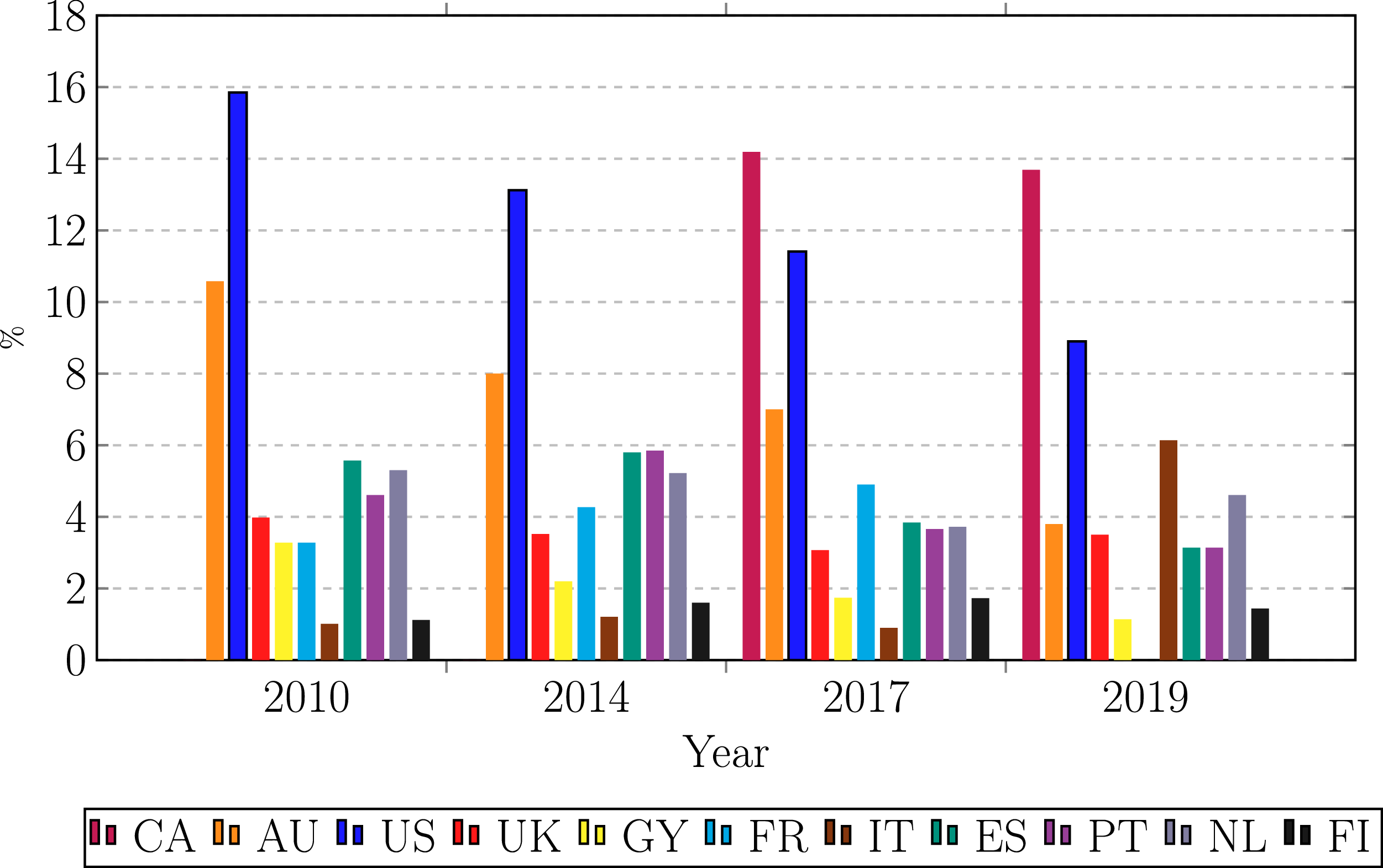
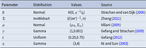

 −
− −
−
 −
− −
−
 p=6
p=6
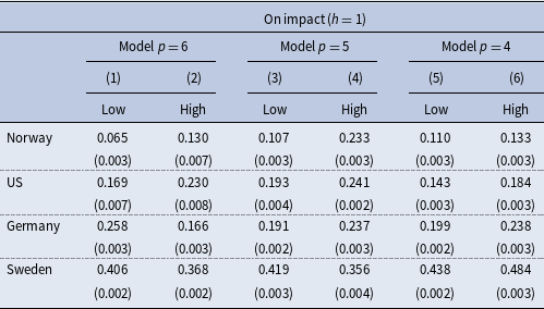

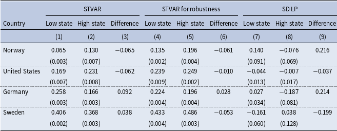


 Open access