3.1 Glacier outlines extraction and attributes calculation

We used data from Landsat complemented by Sentinel-2 and ASTER images (Table S2), where Landsat data were not available or relevant parts of the Landsat scenes were too cloudy or snowy to extract glacier outlines with sufficient accuracy to compute area changes. A total of 12 orthorectified satellite scenes acquired at the end of the ablation season (04 August to 26 September) were used to delineate glacier outlines for the years 1986, 1995, 2005 and 2016 (Fig. S1). Only images with minimum cloud cover and seasonal snow were chosen. All images (Table S2) were retrieved from the USGS (https://glovis.usgs.gov).

The glacier outlines for clean ice were delineated using a semi-automatic procedure based on the band ratio segmentation method (Paul, Reference Paul2000; Albert, Reference Albert2002; Guo and others, Reference Guo2015; Li and others, Reference Li2017). A red/short-wave infrared (R/SWIR) band ratio with a threshold of 2–2.5 (TM3/TM5 of Landsat TM and ETM+, TM4/TM6 of Landsat OLI imagery) and an additional threshold on the blue band (band 1 of TM/ETM+ and band 2 of OLI) digital number were adopted and thresholds were selected interactively (Paul and Kääb, Reference Paul and Kääb2005; Raup and others, Reference Raup2007). We employed sectionalized glacier outline delineation by using moving windows with different optimal band ratio thresholds on the same satellite image to minimize the influence of various snow/ice ablation levels on the optimal thresholds (Guo and others, Reference Guo2015). We also applied a median filter (3 by 3 kernel) to reduce noise in shadowed regions and remove isolated pixels outside the glaciers, although it might reduce the size of small glaciers to some extent (Paul, Reference Paul2002; Andreassen and others, Reference Andreassen, Paul, Kääb and Hausberg2008). Only glaciers with an area ≥0.01 km² were mapped. Following previous studies (Hall and others, Reference Hall, Williams and Bayr1992; Racoviteanu and others, Reference Racoviteanu, Arnaud, Williams and Ordonez2008a; Pan and others, Reference Pan2012; Burns and Nolin, Reference Burns and Nolin2014), debris-covered glacier margins were delineated manually from visual inspection of the images. Clean ice outlines were visually inspected using all available contrast-enhanced false-color composite images as well as Google Earth^TM images to correct errors caused by cast shadow, light clouds and seasonal snow.

Following the top-down method (Guo and others, Reference Guo2015), which identifies the ice divides by aspect differences between the two sides of mountain ridges, we derived ice divides by using the IFSAR DEM, within a 1500 m buffer distance from all glaciers. Results were scrutinized with the help of the shaded relief data and the Landsat scenes, while gross errors were corrected manually where necessary. The ice divides were used to split the glacier complex into individual glaciers.

We extracted a series of glacier-specific attributes including Global Land Ice Measurements from Space (GLIMS)-IDs, coordinates, surface area, debris-covered area, mean slope and aspect, maximum, mean and minimum elevation using the IFSAR DEM and glacier outlines, and added glacier names (if existing) and glacier terminate types (land-terminating, lake-terminating and tidewater) from RGI 6.0. Mean aspect was derived from the arctangent of the mean values of the sine and cosine of the aspect of all DEM cells within a glacier.

3.2 DEM generation and mass change derivation

DEMs derived from ASTER L1A stereo images in 2005 (Fig. 1) and the IFSAR DEM in 2014, were used to compute surface elevation and glacier volume changes over the period 2005–2014. The ASTER data were acquired between 9 August and 14 August, while the IFSAR data were acquired between 29 August and 12 September 2014 (http://viewer.nationalmap.gov/basic/ access date: December 2018, Table S3).

3.2.2 Derivation of ASTER DEMs and bias corrections

The ASTER DEMs were generated from ASTER L1A stereo images (3N and 3B bands) in early August 2005, using the DEM Extraction Wizard of ENVI 5.1 with the geographic reference system NAD83 UTM subregion 5N or 6N (NASA LP DAAC, 2015; Table S3, data downloaded from https://lpdaac.usgs.gov). Since ground control points were not available, more than 200 tie points for each scene, covering different altitudes and surfaces including ice and snow, were automatically collected and then manually examined (removing those influenced by clouds or water) for all stereo-pairs. The maximum Y parallax errors of the tie points were constrained to less than one pixel (±15 m). The DEMs were generated with 30 m resolution. Artifacts, which mainly resulted from clouds and other noises, were removed using a median filter. All extracted ASTER DEMs cover the glacierized area and surrounding terrain within ~10 km from the ice margin.

The resulting DEMs may contain planimetric and altimetric biases (Moore and others, Reference Moore, Holdsworth and Alverson2002; Molnia, Reference Molnia2007; Berthier and others, Reference Berthier, Schiefer, Clarke, Menounos and Remy2010). The DEM biases caused by misregistration between DEMs were corrected by the co-registration method suggested by Nuth and Kääb (Reference Nuth and Kääb2011), which depends on the elevation differences, slope and aspect over stable terrain. The IFSAR DEM was used as master DEM after resampling to 30 m spatial resolution using pixel assembly, and all DEMs (ASTER DEMs and IFSAR DEM) were referenced to the same datum and projection. Only the DEM differences of pixels that do not contain glaciers, water bodies and vegetation (determined by the land cover map of Alaska, USGS (2011)) were used to derive the adjustment coefficients. Then the IQR (see section 3.2.1) was adopted to remove outliers which were typically caused by clouds, data gaps and DEM edges. All iterations of the co-registration adjustment were stopped when the improvement in Std dev. of elevation difference on stable terrain was <2%. Then the along/cross track biases of all ASTER DEMs related to satellite acquisition geometry were corrected using higher order polynomial fittings (5^th to 8^th order; Nuth and Kääb, Reference Nuth and Kääb2011).

Figure 2 illustrates the co-registration of the ASTER DEM (image AST-4, Table S3) to IFSAR DEM. Table 1 and Figure 3 show the co-registration vectors and correction results of each DEM pair.

Fig. 2.

Results of the co-registration of the ASTER DEM (AST-4) to the IFSAR DEM. (a, b) Elevation differences normalized by the slope tangent vs aspect (a) before co-registration and (b) after co-registration, including error bars (blue) and cosine-fit (red line). The fitted equation and coefficient of determination r ² are given in the lower right corner. (c) Residual elevation difference with error bars in the along-track direction. (d) Normal probability density curve of elevation differences. The bin size is 0.0175 (5°) for panels (a) and (b), and 500 and 3 m for panels (c) and (d), respectively.

Fig. 3.

Frequency distribution of elevation changes dh over stable terrain and the glacier area during the study period. Bin size is 3 m. Mean and Std dev. is given for various stages of co-registration (Fig. 2). Panels a, b, c and d refer to the subregions I, II, III and IV (Fig. 1), respectively.

Table 1.

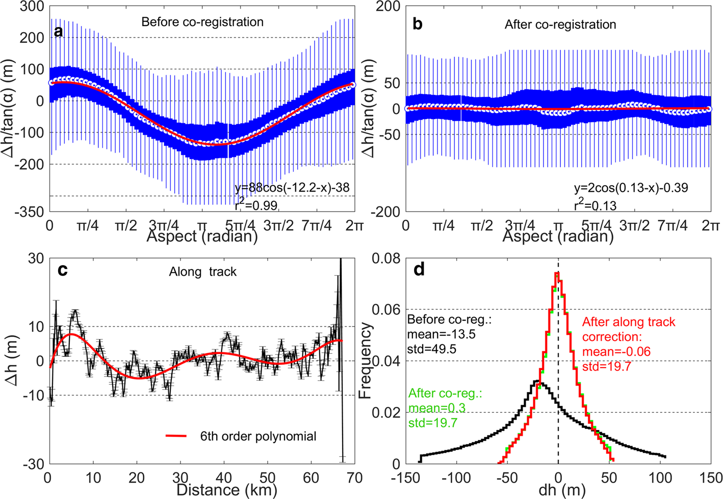
Statistics of elevation differences between ASTER DEMs (AST-1, AST-2a, b, AST-3, AST-4) and IFSAR DEM over stable terrain after co-registration and after additional along/cross track correction. The grid resolution is 30 m. N is the number of pixels, $\overline {\Delta h}$ is the mean elevation difference (m) and σ _non is the Std dev. of elevation difference (m), dx, dy, dz are the three components of the full co-registration adjustment vector (in meters) between the ASTER DEMs and IFSAR DEM.

3.2.3 Elevation changes

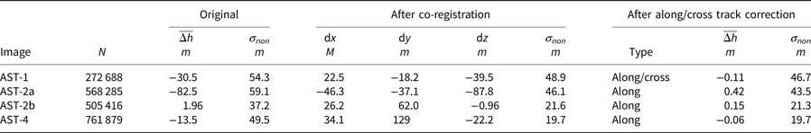
The co-registered ASTER DEMs were subtracted from the IFSAR DEM to calculate elevation difference (dh) over the glacierized areas of the four subregions I–IV (Fig. 1). After scrutinizing the elevation difference maps and difference histograms, we regard pixels with dh dt ⁻¹ values >5 m a⁻¹, < −15 m a⁻¹ for elevations below 1000 m a.s.l. (−10 m a⁻¹ for subregion I) and < −5 m a⁻¹ for elevations higher or equal 1000 m a.s.l. as outliers. This procedure proved to be the most suitable approach in this region compared to other methods, such as empirical value (Berthier and others, Reference Berthier, Schiefer, Clarke, Menounos and Remy2010; Bolch and others, Reference Bolch, Pieczonka and Benn2011), IQR (O'Neel and others, Reference O'Neel, Hood, Arendt and Sass2014; Fischer and others, Reference Fischer, Huss and Hoelzle2015; Kienholz and others, Reference Kienholz2015; Pieczonka and Bolch, Reference Pieczonka and Bolch2015).

Data gaps were filled with the mean value of the elevation change in each 50 m elevation band (Fig. 4), which has been proven as an effective method to interpolate voids in DEM difference maps and can tolerate a rather high percentage of data voids, up to ~60% (McNabb and others, Reference McNabb, Nuth, Kääb and Girod2019).

Fig. 4.

Elevation change rates (blue) for all glacierized cells of ASTER DEMs for which data were available (median ± 1 Std dev.) and area-altitude distribution (50 m bin size) of total glacier area (black), and the area with data gaps (pink). The panels a, b, c and d represent the four subregions I, II, III and IV, respectively (Fig. 1).

3.2.4 Volume and mass change

Glacier volume changes for each subregion and period were computed by multiplying the mean surface elevation changes by the glacier area in 2005 (Tables 2 and 3). A volume to mass conversion factor of 850 ± 60 kg m⁻³ (Huss, Reference Huss2013) was used.

Table 2.

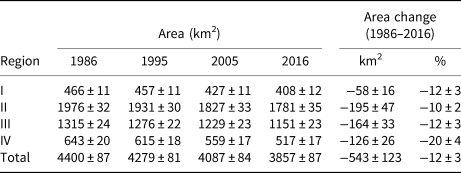
Glacier area in 1986, 1995, 2005, 2016 for four regions (Fig. 1) and the area change 1986−2016

Table 3.

Glacier-wide mean rates of elevation change (dh dt ⁻¹), volume change (dV dt ⁻¹), specific mass change (dM dt ⁻¹) in each subregion (Fig. 1) for 2005–2014. Area refers to the glacier area in 2005. The region-wide average is the area-weighted average of the four subregions

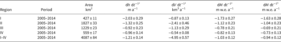
^a Based on original acquisition dates of IFSAR (29 August−12 September 2014) and ASTER DEM (09 August–14 August 2005).

^b Includes correction for seasonal difference in acquisition data, so that the ASTER data refers to 6 September (Section 3.2.4).

3.3 Uncertainty estimation

3.3.1 Glacier outlines

Glacier area errors normally include technical errors (misregistration), interpretation errors and methodological constraints (Raup and others, Reference Raup2007; Paul and Andreassen, Reference Paul and Andreassen2009). In this study, the band ratio method was used to derive almost all glacier outlines from Landsat data and no distinct horizontal shift between images was found when visually checking over stable landforms (e.g. mountain ridges, peaks or lateral moraines), so the technical error was considered negligible and ignored (Bolch and others, Reference Bolch, Menounos and Wheate2010; Guo and others, Reference Guo, Liu, Wei and Bao2013). Interpretation errors are mostly associated with the definition of a glacier, while methodological errors largely depend on the resolution of the source imagery, and the experience of compilers. Following Guo and others (Reference Guo2015), we incorporated all error sources into one term, assuming ±10 and ±30 m accuracies for clean-ice and debris-covered glacier outline delineation respectively, and ±5 m for ice divides.

The buffer method was selected to calculate the uncertainty of glacier area generated from Landsat images, which included both the length of glacier outlines and positional accuracies (e.g. Rivera and others, Reference Rivera, Bown, Casassa, Acuna and Clavero2005; Granshaw and Fountain, Reference Granshaw and Fountain2006; Kienholz and others, Reference Kienholz2015; Tielidze and Wheate, Reference Tielidze and Wheate2018). The area error of each individual glacier E _a, was defined as,

(1)$$E_a = \mathop \sum \limits_{i = 1}^n L_iE_{\,pi}$$

where, i is the type of glacier outlines (clean-ice, debris-covered, ice divides, n = 3) and L _i is the length of glacier outline and E _Pi is the position error. The errors of the position of the ice divides were omitted for considering the whole glacier area of each subregion, and the errors of boundary between clean and debris-covered ice were omitted in the single and regional glacier area error estimation.

The uncertainty of area change E _ΔA over a period t ₁–t ₂, was calculated by

(2)$$E_{\Delta A} = \sqrt {E_{A1}^2 + E_{A2}^2 } $$

where E _A1 and E _A2 are the errors of the glacier area in t ₁ and t ₂, respectively.

3.3.2 Elevation change

Following Zemp and others (Reference Zemp2013) and Huber and others (Reference Huber, McNabb and Zemp2020), the uncertainty of area-averaged elevation change (σ) was estimated from three components: the uncertainty related to spatial autocorrelation in elevation differences (σ _autocorr), the uncertainty related to the residual elevation errors after co-registration (σ _coreg) and the uncertainty due to data voids (σ _void), although this approach may underestimate the total error (Berthier and others, Reference Berthier, Scambos and Shuman2012, Reference Berthier, Cabot, Vincent and Six2016).

(3)$$\sigma = \sqrt {\sigma _{autocorr}^2 + \sigma _{coreg}^2 + \sigma _{void}^2 } $$

The Std dev. of the elevation differences between the ASTER DEMs and IFSAR DEM over nonglacierized pixels (stable terrain; σ _non) can be used as a first estimate of the σ _autocorr, if the spatial correlation of the elevation differences is accounted for (Rolstad and others, Reference Rolstad, Haug and Denby2009). Following Gardelle and others (Reference Gardelle, Berthier, Arnaud and Kaab2013), we calculated the standard error (SE) of the mean elevation change:

(4)$${\rm SE} = \displaystyle{{\sigma _{non}} \over {\sqrt {N_{eff}} }}$$

where N _eff is the effective number of the pixels after de-correlation defined by,

(5)$$N_{eff} = \displaystyle{{N_{tot}\cdot R} \over {2d}}$$

where N _tot is the total number of pixels on the nonglacierized area (stable terrain); R is the pixel size (30 m), d is the de-correlation distance assumed to be 600 m as suggested by Bolch and others (Reference Bolch, Pieczonka and Benn2011) and also used in previous geodetic mass-balance studies (Brun and others, Reference Brun, Berthier, Wagnon, Kääb and Treichler2017; Menounos and others, Reference Menounos2019; Pelto and others, Reference Pelto, Menounos and Marshall2019). σ _autocorr was then calculated using SE and the mean elevation differences of the nonglacier region $\lpar \overline {\Delta h} \rpar$:

(6)$$\sigma _{autocorr} = \sqrt {{\rm S}{\rm E}^2 + {\overline {\Delta h} }^2} $$

σ _coreg was calculated using the triangulation method by Nuth and Kääb (Reference Nuth and Kääb2011). Based on three elevation data sets (ASTER DEM, IFSAR DEM and ICESat), we did co-registration by the correction vectors between each of them and then used the residual between the triangulation of vertical vectors to estimate σ _coreg (Table S6).

The DEM difference maps include data voids encompassing 7, 19, 41 and 1% of the four subregions I, II, III and IV, respectively. Based on findings by McNabb and others (Reference McNabb, Nuth, Kääb and Girod2019), who derived differences to true elevation changes as a function of void percentage, we used the constant values of 0.05 and 0.10 m a⁻¹ to estimate σ _void for subregions II and III, respectively, and assumed zero σ _void for subregions I and IV due to nearly complete coverage.

3.3.3 Errors in volume and specific mass changes

Following standard error propagation, we finally obtained the error of the volume change E _Vol and specific mass balance E _Mass (m w.e. a⁻¹), assuming that error terms are independent of each other by

(7)$$E_{Vol} = \sqrt {{\lpar {dh\cdot E_A} \rpar }^2 + {\lpar {A\cdot \sigma } \rpar }^2} $$

where A is the glacier area in 2005, E _A is the corresponding error.

(8)$$E_{Mass} = \sqrt {{\lpar dh\cdot E_\rho \rpar }^2 + {\lpar \sigma \cdot \rho \rpar }^2} $$

where ρ is the assumed volume to mass conversion factor (850 kg m⁻³), $E_\rho$ is the corresponding error (±60 kg m⁻³); dh is area-averaged surface elevation change, while σ is the corresponding elevation change error (Eqn (3)). The mean annual uncertainty is then given by dividing E _Mass by the number of years.

4.1 Glacier inventory in 2016

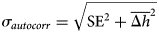
In the 2016 Landsat inventory (L2016), the 1357 glaciers larger than 0.01 km² cover an area of 3857 ± 87 with 35 ± 12 km² (~1%) of the surface debris covered. Half of the glaciers are smaller than 0.1 km², but they contribute only to <1% to the total area. Only 76 glaciers (~6%) are larger than 5 km², however, they make up about 85% of the total area (Fig. 5a).

Fig. 5.

Characteristics of glacier distribution of Kenai Peninsula in 2016. (a) Distribution of glaciers in different area classes; (b) scatterplot of glacier size vs maximum and minimum elevation (Max. elev., Min. elev.). The solid lines (blue and pink) give mean values for distinct size classes while the dark line shows the median elevation per area class for the same area classes as shown in (a); (c) Mean elevation vs aspect per glacier; the solid line refers to the mean per cardinal sector; (d) Mean slope vs glacier size per glacier. The solid line shows the trend (2^nd polynomial fit). X-Axis in (b) and (d) is logarithmically transformed.

Figure 5b indicates that the glaciers' minimum elevation decreases while their maximum elevation increases as the glacier size increase, indicating that glaciers reaching sea-level require a large elevation range, similar to the findings on southern Baffin Island (Paul and Svoboda, Reference Paul and Svoboda2009). The median elevation of all glaciers fluctuates slightly around ~1100 m a.s.l., regardless area class which may indicate that the equilibrium line of the Kenai Peninsula glaciers is at a similar elevation. There is no correlation between mean glacier elevation and aspect (Fig. 5c). As expected, the mean glacier slope decreases with glacier size, but the scatter is large for smaller glaciers (Fig. 5d) due to local topography (Haeberli and Hoelzle, Reference Haeberli and Hoelzle1995; Paul and others, Reference Paul, Frey and Le Bris2011).

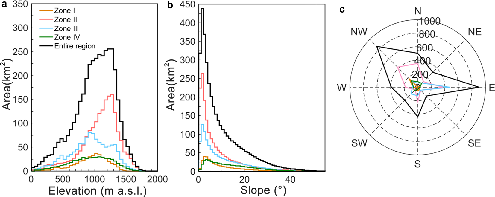
Figure 6 illustrates the area distribution per elevation, slope and aspect class for each subregion as well as the entire region. Nearly all ice-covered area (>99%) is situated between 150 m and 1750 m a.s.l. (Fig. 6a). The area-elevation distribution of subregion II peaks at a higher elevation than the remaining regions. As shown in Figure 6b, glacier area with slopes <30° occupies 90% of the total area. Figure 6c indicates that there is a tendency for glacierized pixels in all subregions to face towards the northwest or east.

Fig. 6.

Area distribution of topography variables for glacierized area in each subregion (I, II, III and IV) and the entire region in 2016 including (a) hypsography with bin size 50 m, and (b) slope with bin size of 1°; (c) aspect, in which numbers represent the glacier area with unit km² in 22.5° aspect bins.

4.2 Area change

Total glacier area has shrunk by 543 ± 123 km² (12 ± 3%) between 1986 and 2016. Glaciers in different regions retreated at different speeds (Table 2) and the highest area loss rate occurred in subregion IV (total area loss of 20 ± 4%).

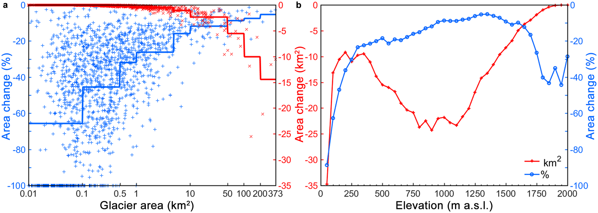
Larger glaciers tend to have smaller relative area losses than smaller glaciers, but the scatter especially for the smaller glaciers is large (Figs 7a, 8b), consistent with previous studies (Maisch and others, Reference Maisch, Haeberli, Hoelzle and Wenzel1999; Serandrei Barbero and others, Reference Serandrei Barbero, Rabagliati, Bianghi and Rampini1999; Kääb and others, Reference Kääb, Paul, Maisch, Hoelzle and Haeberli2002; Paul, Reference Paul2002; DeBeer and Sharp, Reference DeBeer and Sharp2009; Bolch and others, Reference Bolch, Menounos and Wheate2010). The average area loss for glaciers <0.5 km² is nearly 56%, ranging from 0 to 100%, while it is 8% for glaciers larger than 10 km². Approximately 270 glaciers (all <0.5 km²) disappeared during 1986–2016. Larger retreat rates of smaller glaciers can be attributed to a stronger impact of local topographic characteristics on the processes controlling the glacier mass balance (Florentine and others, Reference Florentine, Harper, Fagre, Moore and Peitzsch2018). For example, a moderate rise in the equilibrium line may turn the entire glacier to ablation zone (Kaser and Osmaston, Reference Kaser and Osmaston2002; Racoviteanu and others, Reference Racoviteanu, Williams and Barry2008b). A given specific mass change may also result in larger relative area changes for smaller and thinner glaciers than larger glacier with steeper flanks (Kääb and others, Reference Kääb, Paul, Maisch, Hoelzle and Haeberli2002). Generally, the area loss rate decreases with increasing elevation (Fig. 7b) except for elevations above 1700 m a.s.l. where the sample size is very small and errors most likely larger due to steep terrain, cast shadows and seasonal snow.

Fig. 7.

(a) Relative (blue) and absolute (red) glacier area change between 1986 and 2016 (a) for each glacier (n = 1660) as a function of glacier area, and (b) as a function of elevation (based on all glacier pixels falling within sequential 50 m bins). Solid lines in (a) show the mean values per area class.

Fig. 8.

(a) Glacier area-elevation distribution for four different years, and (b–d) glacier area-change rates for different periods between 1986 and 2016 vs (b) area size class, (c) mean slope and (d) aspect. The bin size in panel a is 50 m. Numbers in panel d refer to area change rates in % (10 a)⁻¹.

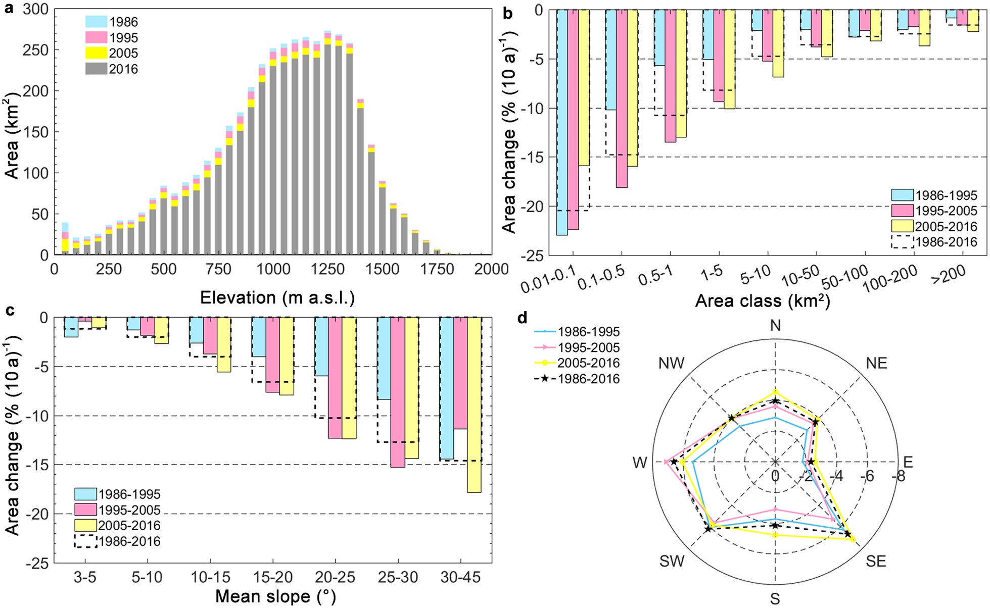
For glaciers smaller than 0.1 km² (nearly 50% of the total number of glaciers) with a more notable reduction in area than others, the area loss during 2005–2016 is markedly lower than during the earlier periods of 1986–1995 and 1995–2005 (Fig. 8b). One possible explanation is that small glaciers may retreat into more sheltered locations that facilitate their preservation (DeBeer and Sharp, Reference DeBeer and Sharp2009).

We investigated the role of the slope and aspect in spatial variations in area change. Results show that slope played an important role in relative glacier area reduction. Glaciers located on steeper terrains experienced larger relative area loss than less steep glaciers (Fig. 8c) consistent with previous studies (Salerno and others, Reference Salerno, Buraschi, Bruccoleri, Tartari and Smiraglia2008; Racoviteanu and others, Reference Racoviteanu, Arnaud, Williams and Manley2015; Tielidze and Wheate, Reference Tielidze and Wheate2018). Southeast-south-southwest facing glaciers experienced generally more pronounced shrinkage than northwest-north-northeast facing glaciers. This is similar to the pattern found in the Himalaya by Ahmad and Rais (Reference Ahmad and Rais1999), which was attributed to more solar radiation on the south-facing than north-facing slopes.

4.3 Glacier elevation and mass changes

Figure 9 shows the spatial distribution of surface elevation changes for the four subregions during 2005–2014. All regions experienced most pronounced thinning in the lower parts especially below 1000 m a.s.l., and less pronounced thickening or thinning in the glaciers' upper reaches.

Fig. 9.

Spatially distributed surface elevation changes rates for the period 2005–2014. Dark gray areas represent the cloud error mask of the ASTER DEM, while white area with blue dashes mark the areas with no data. The red line is the 1000 m contour line. The panels a, b, c and d represent the four subregions I, II, III and IV, respectively (Fig. 1).

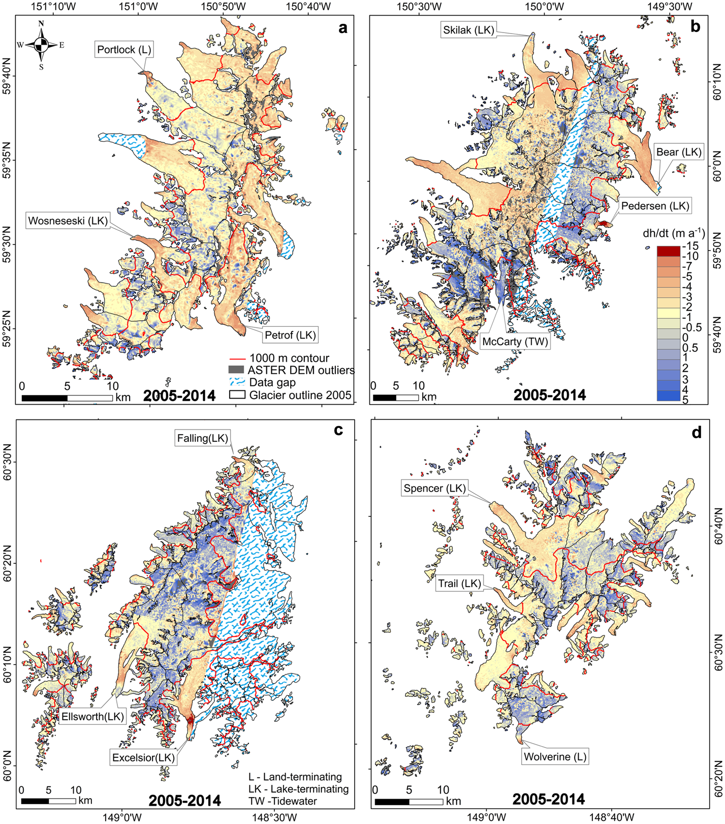
In subregion I (Grewing-Yalik glacier complex), most thickening occurred above 1000 m a.s.l., but the lower tongue of Portlock Glacier and some smaller glaciers in the southeast show some thickening at lower elevations (Fig. 9a). In subregion II (Harding Icefield), especially the upper reaches of some glaciers in the southwest and southeast experienced thickening. It remains unclear whether this thickening is caused by net snow accumulation, changes in ice dynamics or by errors due to the noise of ASTER DEM (Fig. 9b). Large parts of McCarty Glacier (<1000 m a.s.l.) show a positive surface elevation change, similar to results found by Aðalgeirsdóttir and others (Reference Aðalgeirsdóttir, Echelmeyer and Harrison1998) for the period 1950s–1990s.

The two lake-terminating glaciers (Falling and Excelsior glacier), experienced extreme thinning close to their termini (nearly 15 m a⁻¹). The lower tongue of Ellsworth Glacier shows glacier thickening during the studied period (Fig. 9c). However, based on recent satellite imagery, no evidence of a surge could be detected that could explain the local thickening. More studies, such as the surface velocity and its recent dynamics, or the distribution of its thickness, are needed to reveal its causes. Errors in the DEMs may also explain this anomaly.

The regional elevation and mass changes during 2005–2014 for the four subregions are given in Table 3. Results emphasize the need to correct for differences in acquisition dates of any two DEMs to be differenced in regions with considerable mass change over short periods. Without accounting for the 27-days elevation difference between the ASTER DEMs and IFSAR DEM acquisition date, the area-average region-wide mass-balance rate would have been underestimated by 0.09 m w.e. a⁻¹ (~10%).

On average the glaciers on the Kenai Peninsula experienced specific mass changes of −0.94 ± 0.12 m w.e. a⁻¹. Mass-balance rates were most negative for lake-terminating glaciers (−1.37 ± 0.13 m w.e. a⁻¹, ~980 km²), followed by land-terminating glaciers (−1.02 ± 0.13 m w.e. a⁻¹, ~2166 km²) and tidewater glaciers (−0.45 ± 0.14 m w.e. a⁻¹, ~941 km²). This pattern cannot be explained with differences in mean elevation (Table 4). Many lake- or marine-terminating glaciers experienced pronounced thinning especially on their tongues (Wosneseski, Petrof, Skilak, Bear, Pedersen, Falling, Excelsior, Spencer and Trail glaciers; Fig. 9), but not all (for example McCarty glacier). This trend is consistent with airborne laser altimetry derived results across Alaska (Larsen and others, Reference Larsen2015), which indicated more rapid thinning of many lake-terminating glaciers near their termini compared to land-terminating glaciers.

Table 4.

Area (% of total), mean elevation and specific mass balance (dM dt ⁻¹ in m w.e. a⁻¹) during the period 2005–2014 for three glacier types (land-terminating, lake-terminating and tidewater glaciers) in each subregion (Fig. 1). Area refer to the inventory from 2005 and elevations to the IFSAR DEM in 2014

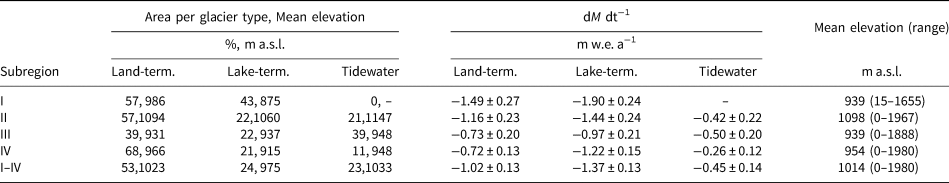
Mean specific mass change rates varied considerably among the four subregions (Table 3). Subregion I (Grewing-Yalik glacier complex) experienced the most negative mean mass change (−1.63 ± 0.28 m w.e. a⁻¹), and subregion III (Sargent Icefield) the least negative rate (−0.69 ± 0.21 m w.e. a⁻¹). These differences are consistent with the relative distribution of glacier types. Subregion I has roughly twice as much lake-terminating glacier area (in %) than the other subregions while tidewater glaciers are lacking. In contrast subregion III has a considerably higher percentage of tidewater glacier area compared to the other regions (Fig. 1, Table 4).

Wolverine glacier (~17 km², Fig. S3), located in subregion IV and part of the USGS benchmark glacier monitoring project, had an average glacier-wide mass-balance rate of −0.55 m w.e. a⁻¹ during the period 2005–2014 (O'Neel and others, Reference O'Neel2019), is similar to the averaged mass-balance rate of subregion IV (−0.73 ± 0.13 m w.e. a⁻¹). However, we find a less negative mass-balance rate for Wolverine glacier for the same period (−0.20 ± 0.13 m w.e. a⁻¹) and attribute this discrepancy to artifacts in the DEMs which are introduced by the steep local topography (Koblet and others, Reference Koblet2010; Le Bris and Paul, Reference Le Bris and Paul2015).

4.4 Comparison with other studies

Our new Landsat derived glacier inventory of the Kenai Peninsula for 2005 includes 1421 glaciers covering an area of 4087 ± 84 km², which agrees well with RGI 6.0 (1457 glaciers, ~4175 km², Kienholz and others, Reference Kienholz2015) compiled in 2005–2007. Hall and others (Reference Hall, Giffen and Chien2005) found an area reduction of 3.6% (~78 km²) for the Harding Icefield and Grewingk-Yalik Glacier Complex (excluding the glaciers in the surroundings that are not connected to these ice fields) over the time interval 1986–2002. Their results are similar to our results for 1986–2005 for the same ice masses (area loss of 91 ± 22 km², 4.2%). O'Neel and others (Reference O'Neel2019) found that the Wolverine glacier experienced a 1.5 km² area reduction between 1969 and 2018, which is similar to the area loss of 1.4 km² found in this study for the period 1986–2016.

Aðalgeirsdóttir and others (Reference Aðalgeirsdóttir, Echelmeyer and Harrison1998) calculated a surface thinning rate for the Harding Icefield (subregion II) of −0.49 ± 0.12 m a⁻¹ for the period 1950s–1996, which is close to the rate of −0.47 ± 0.01 m a⁻¹ found by VanLooy and others (Reference VanLooy, Forster and Ford2006) for roughly the same period (1950 to mid-1990s). The latter study found an accelerated rate of surface elevation change (−0.72 ± 0.13 m a⁻¹) in the period mid-1990s to 1999. For the glaciers in subregions I and II combined, they report a surface elevation change rate of −0.61 ± 0.12 m a⁻¹ for the entire period 1950–1999. Correspondingly, we find accelerated elevation change rates of −1.97 ± 0.29 and −1.26 ± 0.25 m a⁻¹ for subregions I and II (the area-average value is −1.39 ± 0.21 m a⁻¹), respectively, for the period 2005–2014.

For the entire Kenai Range (subregions I-IV, Fig. 1), our results (−0.94 ± 0.12 m w.e. a⁻¹) are considerably more negative than the mass-balance rates of −0.06 ± 0.40 m w.e. a⁻¹ from 1994/1996 to 1999/2001 reported by Arendt and others, Reference Arendt, Walsh and Harrison2009, and −0.45 ± 0.11 m w.e. a⁻¹ between 1962 and 2006 found by Berthier and others, Reference Berthier, Schiefer, Clarke, Menounos and Remy2010, suggesting that glaciers mass loss in the Kenai Peninsula has strongly accelerated since at least the mid-2000s. These findings are in agreement with observed acceleration of glacier mass loss in Western Canada between the periods 2009–2018 and 2000–2009 (Menounos and others, Reference Menounos2019).

Our results are also more negative than regional-scale estimates in other regions in Alaska during similar periods, for example, on the Juneau Icefield and the Stikine Icefield (−0.68 ± 0.15 and −0.83 ± 0.12 m w.e. a⁻¹, respectively) over the period 2000–2016 (Berthier and others, Reference Berthier, Larsen, Durkin, Willis and Pritchard2018) and also averaged over all glaciers in Alaska and adjacent Yukon (−0.69 ± 0.18 m w.e. a⁻¹) for the period 2006–2015 (Hock and others, Reference Hock, Pörtner, Roberts, Masson-Delmotte, Zhai, Tignor, Poloczanska, Mintenbeck, Alegría, Nicolai, Okem, Petzold, Rama and Weyer2019).

4.5 Regional climate variability and trends

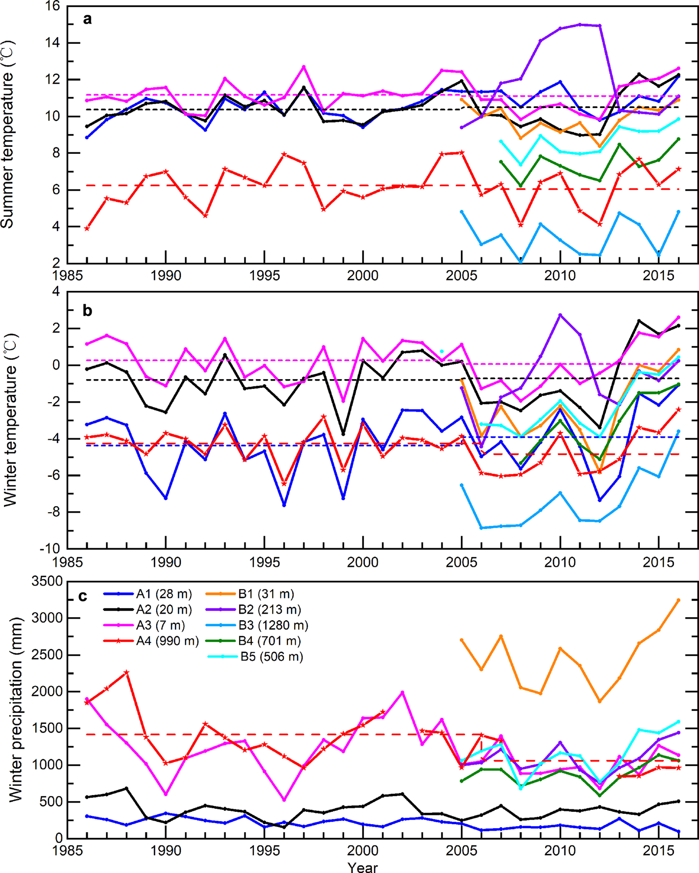
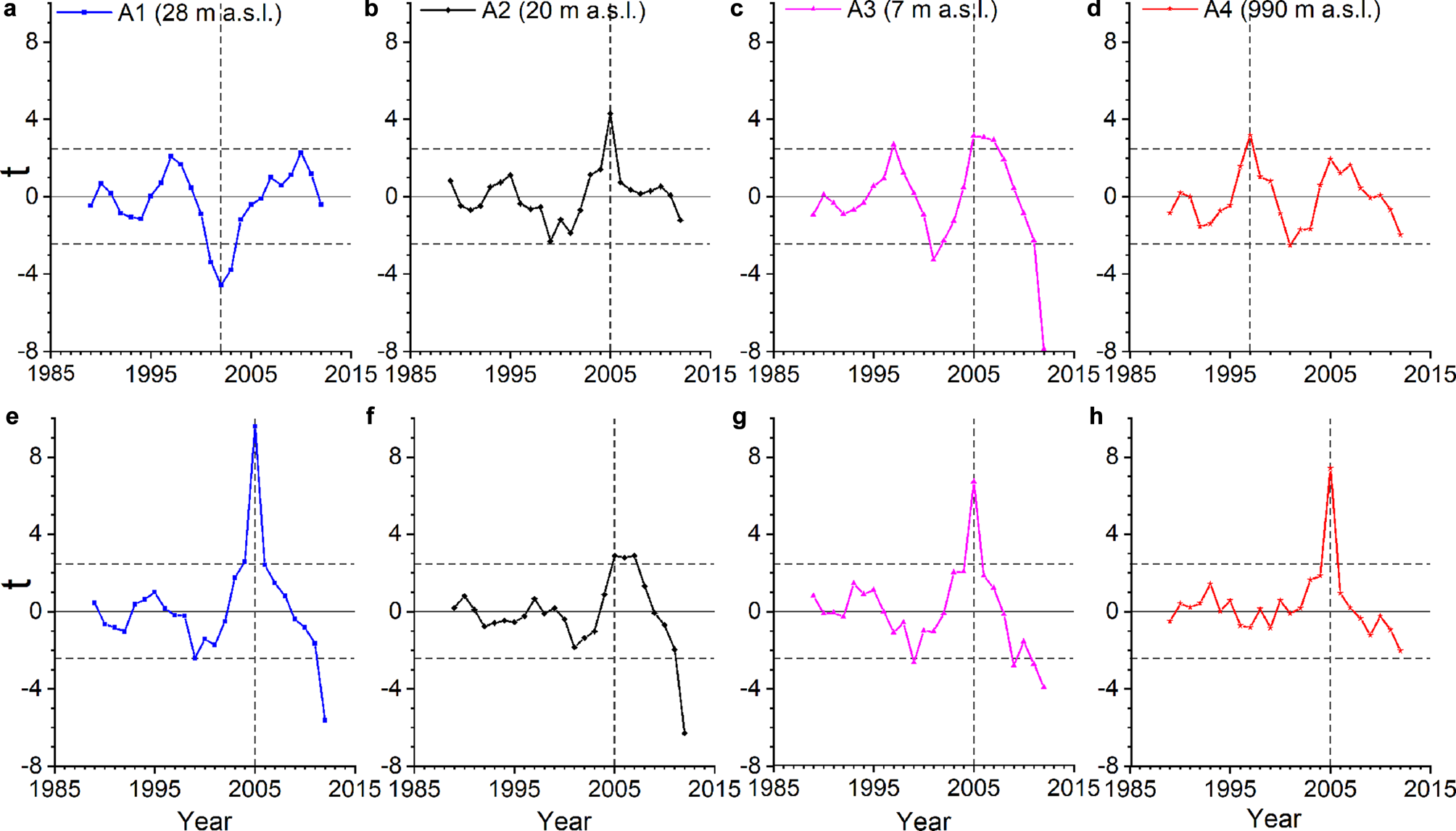
To investigate the causes of the accelerated glacier mass losses we analyzed air temperature and precipitation records on the Kenai Peninsula (Fig. 10, Table S7). Only four weather stations (A1, A2, A3, A4; Fig. 1) have longer than 30 years of largely uninterrupted observations through at least 2016, while data from the other five stations close to the ice masses (B1–B5, Fig. 1) are only available since 2005. All records show large interannual variation for both air temperature and precipitation (Fig. 10). We applied a moving t-test (Afifi and Azen, Reference Afifi and Azen1972; Fu and others, Reference Fu, Diaz, Dong and Fletcher1999) to the summer and winter temperature data to explore possible abrupt changes in temperature. Results indicate a significant change (at significance level α = 0.05) in 2005 for all stations, except for summer temperature at A1 and A4, where the change occurred in 2002 and 1997, respectively (Fig. 11).

Fig. 10.

Time series of (a) summer (May to September) temperature, (b) winter (October to April) temperature and (c) winter (October to April) precipitation for eight weather stations in the Kenai Peninsula (Fig. 1) in the period 1986–2016. Dotted lines are the mean values before and after 2005 when an abrupt change was detected with statistical significance α = 0.05 (Fig. 11). Numbers in parentheses indicate the elevation of each weather station (m a.s.l.). Precipitation data are not available for B3. Data from NOAA, except A4 (Wolverine weather station), from the USGS.

Fig. 11.

The moving t-test curve of the air temperatures of four weather stations (A1, A2, A3 and A4) on the Kenai Peninsula. Dashed horizontal lines indicate the 95% confidence level (α = 0.05). Results indicate an abrupt change in 2005 (or 2002 in panel a, 1997 in b). Panels a–d refer to summer temperatures, while panels e–h refer to winter temperatures.

We calculate temperature trends for the period 2005–2016 for the five stations (B1–B5) that lack prior data and over the period 1986–2016 for the four stations (A1–A4) with longer records. Except for station A1 (1986–2016) and station B1 (2005–2016) linear warming trends in summer are not significant (Table S7). Three stations (B3, B4 and B5) show pronounced positive linear trends in winter temperature over the period 2005–2016, however, trends for the stations (A1–A4) going back to 1986 are not significant. In fact, mean summer and winter temperatures of the periods 1986–2005 and 2005–2016 are similar (Fig. 10). Precipitation variations are complex with both positive and negative trends, but only two stations (A1 and A4) have trends (negative) over the period 1986–2016 that are significant (p < 0.05, Table S7). Although decreasing precipitation is consistent with accelerated mass loss, the precipitation records are too short and scarce, especially at high elevation, to elucidate the role of precipitation in the observed glacier changes.

Overall, the large interannual variability and mostly short air temperature and precipitation records with largely insignificant changes of most of the investigated records hamper unambiguous attribution of the observed accelerated specific mass losses of the glaciers on the Kenai Peninsula during 2005–2014 compared to earlier periods covered in previous studies. In addition, changes in frontal ablation (calving and submarine melt) of tidewater glacier due to changes in ocean properties close to the calving fronts may also have contributed to accelerated mass loss, but their role remains unknown.