

1. INTRODUCTION
According to the International Maritime Organization (IMO, 2009a) and Food and Agriculture Organization of the United Nations (FAO, 2012), globally, there were around 70 000 merchant ships sailing for world trade and about 4·36 million fishing vessels with nearly 2·6 million engine-powered in 2010. Among the motorised fishing vessels, about 1·8 million were operated in sea waters and others were operated in inland waters. In 1997, the IMO adopted a resolution on CO2 emissions from ships. Afterwards, the Marine Environment Protection Committee (MEPC) developed a greenhouse gas emission index for ships (IMO, 2009a). The MEPC published guidelines for the use of an Energy Efficiency Operational Indicator (EEOI), which provides useful information on ship's performance with regard to fuel efficiency. The EEOI is currently for voluntary use by each ship. Recently, the IMO (2012) has started to require the Energy Efficiency Design Index (EEDI) for new ships, and the Ship Energy Efficiency Management Plan (SEEMP) for all ships. These documents list various options to improve energy efficiency such as speed optimisation, weather routing, and hull maintenance (IMO, 2012). The optimum speed represents the speed at which minimum fuel usage per tonnage mile is reached. Speed optimisation can yield significant savings and consideration of the engine manufacturer's power curve and the ship's propeller curve should be incorporated. Generally, a 10% decrease of ship speed will result in 19% reduction of engine power and 27% reduction of energy consumption and therefore reduction in CO2 emissions (IMO, 2010). Weather routing is available for all types of ship, and has a high potential for energy efficiency. Ship routing often considers ocean weather associated with eddies, meanders, storm likelihood, ocean surface waves, sea ice and tides. Optimising ship routes not only reduces CO2 emissions but also reduces emissions of NOx, black carbon and SO2, which will impact on climate and health. For hull maintenance, the smoother the hull, the better fuel efficiency. Propeller cleaning and polishing can significantly increase fuel efficiency. According to IMO (2009a; 2009b; 2011), other technologies are also expected to be used for reducing fuel consumption such as improvement of engine efficiency, reducing on-board power demand, optimisation of ship handling, solar power, and wind power, etc.
Application of favourable ocean currents can also reduce a ship's energy consumption (Lo and McCord, Reference Lo and McCord1995; Chang et al., Reference Chang, Tseng, Chen, Chu and Shen2013b). Usually, strong ocean currents exist near the western boundary of ocean basins, and are called the Western Boundary Currents (WBCs) such as the Gulf Stream in the North Atlantic and the Kuroshio in the North Pacific. In addition, swift surface flows can be sometimes induced by high wind speeds or tropical cyclones (Chang et al., Reference Chang, Tseng and Centurioni2010; Reference Chang, Chen, Tseng, Centurioni and Chu2012; Reference Chang, Chen, Tseng, Centurioni and Chu2013a). Lo and McCord (Reference Lo and McCord1995) estimated that 5–8% fuel savings can be achieved for ships traveling with the Gulf Stream at sailing speeds of about 16 knots. Chang et al. (Reference Chang, Tseng, Chen, Chu and Shen2013b) suggested a fuel reduction of 2–6% for vessels sailing with the Kuroshio Current between Taipei and Tokyo at an average speed of 12 knots. Effective use of these strong currents can yield huge savings considering that a large number of engine-powered fishing boats worldwide move at speeds of about 6–10 knots. The energy savings are even more obvious for ships with a lower cruising speed when taking into account strong ocean currents. The typical flow speeds of WBCs are approximately 2–3 knots, which is equivalent to 33–50% of the ship speeds of small fishing boats. Thus, smaller fishing boats will save more fuel, time and money, and reduce greenhouse gas emissions if they effectively utilise strong ocean currents. Questions arise: Do captains of all vessels know the correct locations of these strong currents for optimal route planning? Can a global map of strong currents be constructed from a relatively long time series of current data? How significant is the fuel saving after the detailed ocean circulation mapping is constructed and utilised? The goal of this study is to answer these questions, and to provide an energy-saving map with strong currents for all types of ships. The study will also focus on ship's characteristics to present the impact on navigation (i.e. ship's particulars) based on strong ocean currents. To do so, global current data from satellite measurements are used to represent a detailed and complete map of strong currents.
2. DATA
In this study, geostrophic currents of 1992–2012 from a merged product of TOPEX/Poseidon, Jason 1, and European Research Satellite altimeter observations are used to examine the global ocean surface circulation. Produced by the French Archiving, Validation, and Interpolation of Satellite Oceanographic Data (AVISO) project using the mapping method of Ducet et al. (Reference Ducet, Le Traon and Reverdin2000), the total geostrophic currents can be obtained from the AVISO website (http://www.aviso.oceanobs.com/index.php?id=1271). The data processing of AVISO using optimal interpolation with realistic correlation functions generates a combined map merging measurements from all available altimeter missions (Ducet et al., Reference Ducet, Le Traon and Reverdin2000). The combined data from all altimeter missions can greatly improve the estimation of mesoscale signals. The data are interpolated onto a global grid of 1/3° resolution between 82°S and 82°N and are archived in weekly (7 days) averaged frames. The geostrophic currents are calculated from the absolute dynamic topography, which consists of a Mean Dynamic Topography (MDT) and the anomalies of the altimeter sea level. Rio and Hernandez (Reference Rio and Hernandez2004) have explained in detail the method of estimating the MDT. The resulting geostrophic currents have been validated with independent drifter data to have a root-mean-square difference of about 14 cm/s in the Kuroshio area (Rio and Hernandez, Reference Rio and Hernandez2004). Readers are referred to Le Traon et al. (Reference Le Traon, Nadal and Ducet1998), Le Traon and Dibarbour (Reference Le Traon and Dibarboure1999), Le Traon et al. (Reference Le Traon, Dibarboure and Ducet2001), Pascual et al. (Reference Pascual, Faugere, Larnicol and Le Traon2006), Ducet et al. (Reference Ducet, Le Traon and Reverdin2000) and Qiu and Chen (Reference Qiu and Chen2006) for more details on the data analysis method.
3. GLOBAL STRONG OCEAN CURRENTS
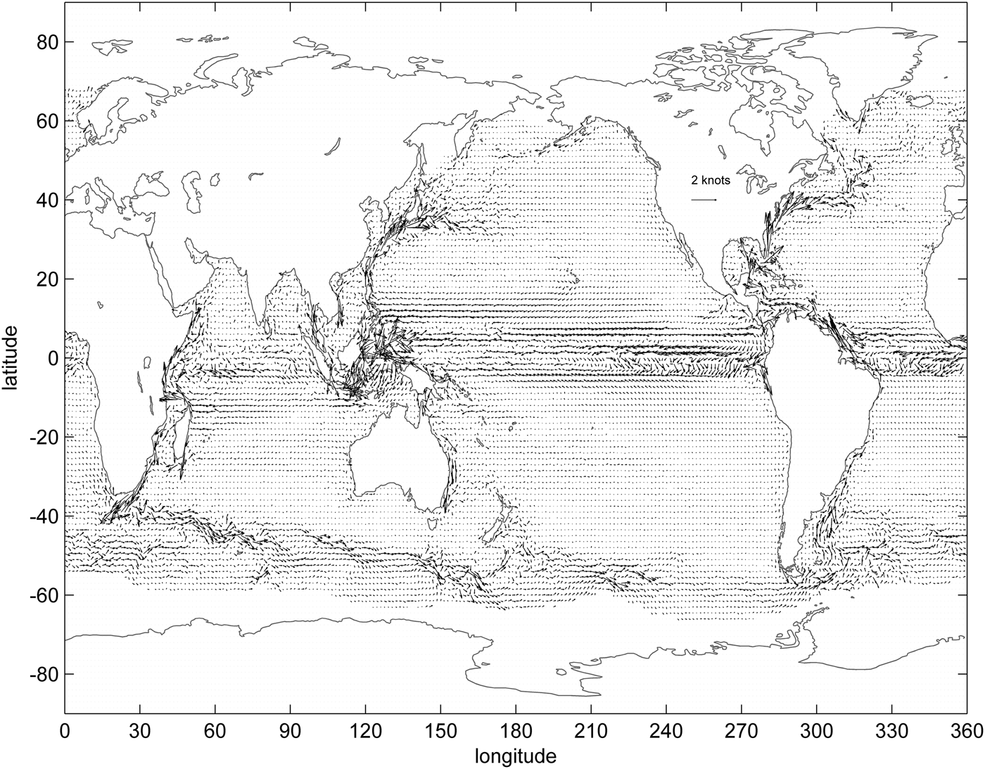
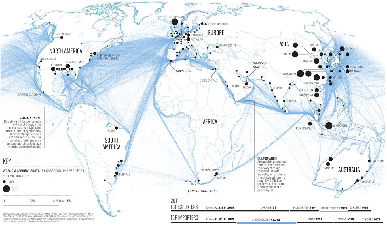
Figure 1 shows the global ocean bathymetry derived from ETOPO2. The mean current speeds and vectors averaged from AVISO data of 1992–2012 in 1/3° × 1/3° bins are shown in Figures 2 and 3, respectively. Strong currents (~2 knots) can be clearly seen to occur in the six red boxes of Figure 2 (marked as a-f), with their locations at the North America, South America, Northeast Asia, Southeast Asia, Australia, and Africa, respectively. Most of the strong currents are typical WBCs in the Pacific, Atlantic and Indian Ocean. WBCs and Eastern Boundary Currents (EBCs) are ocean currents with dynamics determined by the presence of a coastline. The WBCs of a basin are stronger than EBCs. Based on the conservation of mass and potential vorticity, the transport is balanced by a narrow and strong current, which flows along the western boundary of the basin (Stommel, Reference Stommel1948; Munk, Reference Munk1950). A global, detailed and complete map of strong ocean currents, expressed in speed magnitude and vector, is shown in Figures 2 and 3, respectively compiled from a relatively long period (21 years) of satellite altimeter observations and averaged in 1/3° × 1/3° bins. Figures 2 and 3 can be utilised for the purpose of ship routing. The relative density of global commercial shipping for various shipping routes is shown in Figure 4 (Halpern et al., Reference Halpern, Walbridge, Selkoe, Kappel, Micheli, Agrosa, Bruno, Casey, Ebert, Fox, Fujita, Heinemann, Lenihan, Madin, Perry, Selig, Spalding, Steneck and Watson2008; Wikipedia website, 2014). A significant portion of the shipping routes could be seen to be within the regions of strong currents. In order to provide ship routers with more details of the primary path of these strong ocean currents at various locations, enlargements of mean current vectors are plotted in Figures 5(a), 6(a), 7(a), 8(a), 9(a), and 10(a) for the Northwestern Atlantic, western Equatorial Atlantic, Northwestern Pacific, western Equatorial Pacific, Southwestern Pacific, and western Indian Ocean (the six red boxes in Figure 2), respectively. For comparison purposes, the commercial shipping routes at each region are also plotted in Figures 5(b), 6(b), 7(b), 8(b), 9(b), and 10(b). As described earlier, most of the previous shipping routes might not take the strong ocean currents into consideration, and this fact can be clearly seen in the comparison between graphs of ship routing and ocean currents.
Geography and bottom topography of the world oceans derived from ETOPO2.

Averaged speeds of total geostrophic currents in 1/3° × 1/3° bins of the world oceans (1992–2012). Six red boxes labelled a-f indicate regions of strong ocean currents.
Averaged total geostrophic velocity vectors in 1/3° × 1/3° bins of the world oceans (1992–2012).
Map of global shipping routes illustrates the relative density of commercial shipping (Halpern et al., Reference Halpern, Walbridge, Selkoe, Kappel, Micheli, Agrosa, Bruno, Casey, Ebert, Fox, Fujita, Heinemann, Lenihan, Madin, Perry, Selig, Spalding, Steneck and Watson2008; Wikipedia website, 2014).
(a) Bin-averaged velocity and (b) shipping routes in the western North Atlantic. The isobaths are 500, 2000, and 4000 m in (a).
(a) Bin-averaged velocity and (b) shipping routes in the western tropical Atlantic and eastern tropical Pacific. The isobaths are 500, 2000, and 4000 m in (a).
(a) Bin-averaged velocity and (b) shipping routes in the western North Pacific. The isobaths are 500, 2000, and 4000 m in (a).
(a) Bin-averaged velocity and (b) shipping routes in the western Equatorial Pacific. The isobaths are 500, 2000, and 4000 m in (a).
(a) Bin-averaged velocity and (b) shipping routes in the western South Pacific near Australia. The isobaths are 500, 2000, and 4000 m in (a).
(a) Bin-averaged velocity and (b) shipping routes in the western South Indian Ocean. The isobaths are 500, 2000, and 4000 m in (a).
4. STRONG CURRENTS IN THE ATLANTIC
The enlarged map of Figure 5(a) and 5(b) shows the average flow path (direction and strength) of the WBC and shipping routes in the north western Atlantic. The Yucatan Current, which flows northward through the Yucatan Channel (a passage between Mexico and Cuba), enters the Gulf of Mexico. Strong surface currents of 2 knots are found to exist on the western side of the Yucatan passage. A loop current is formed along the 500 m isobaths in the Gulf of Mexico. Waters flow out from the Gulf of Mexico into the Atlantic through the Florida Strait as the Florida Current. The Florida Current joins the Gulf Stream off the east coast of Florida, and flows northward along the east coast of the United States. Maximum current speeds of the Gulf Stream and the Florida Current reach 3 knots or more. Some shipping routes seem to ride favourable currents along the east coast of the United States, but most of the routes were apparently based on the shortest distance between two ports. Lo and McCord (Reference Lo and McCord1995) suggested that in the Gulf Stream region average fuel savings of 7·5% can be achieved for vessels riding favourable currents, and the fuel savings are 4·5% if vessels with an average speed of 16 knots avoids adverse current flows.
In the western equatorial Atlantic, the broad westward flowing South Equatorial Current (SEC) current, which extends from the surface to about 100 m depth, approaches the Brazilian coast. The SEC splits into two branches near 10°S (Silveira et al., Reference Silveira, de Miranda and Brown1994). The stronger branch, called the North Brazil Current (NBC), flows northward along the Brazil coastline (Figure 6(a)) and the weaker branch flows southward as the Brazil Current. The NBC merges with a northern branch of the SEC at around 5°S, and the northward flow speed strengthens to 2 knots just north of the Amazon estuary. Another fast flow worth mentioning is observed off Central America, along the northern coast of Panama and Costa Rica, with a strong westward flow of 1·6 knots.
5. STRONG CURRENTS IN THE PACIFIC
The Kuroshio Current (KC) is the WBC of the North Pacific gyre (Yamashiro and Kawabe, Reference Yamashiro and Kawabe1996; Hsueh et al., Reference Hsueh, Schultz and Holland1997; Ambe et al., Reference Ambe, Imawaki, Uchida and Ichikawa2004; Yuan et al., Reference Yuan, Han and Hu2006). Figure 7(a) shows an enlarged map of the KC path and velocities between Taiwan and Japan. The average velocity of the KC along the east coast of Taiwan is about 2 knots, while the velocity of KC increases to 2·7 knots along the south coast of Japan. A recent study by Chang et al. (Reference Chang, Tseng, Chen, Chu and Shen2013b) also compiled a complete track of strong ocean currents in the northwestern Pacific from the Surface Velocity Program (SVP) drifter current data, with the focus on Kuroshio, as a potential energy-saving route for vessels in this region. In order to provide not only mean speed of the KC but also some information on measurement uncertainty and variability of currents, a comparison between Figure 1 of Chang et al. (Reference Chang, Tseng, Chen, Chu and Shen2013b) and Figure 7(a) of this study was made. It should be noted that drifter-measured velocities include small length-scale (small-scale eddy) and short time-scale (tidal current…etc) components. Also note that drifter-measured velocity is at 15 m depth while absolute geostrophic velocity estimated from satellite sensors is at the sea surface. The comparison indicates that the primary track and velocities of KC from both studies are generally very similar and consistent, except for some subtle changes of KC axis revealed by Chang et al. (Reference Chang, Tseng, Chen, Chu and Shen2013b).
In 2011, the top five exporters are China, Japan, Saudi Arabia, United States, and South Korea (http://www.ritholtz.com/blog/wp-content/uploads/2012/05/map.png), and the top five importers are China, United States, Japan, Taiwan, and South Korea. Overall, strong economic activities take place in the Asian Pacific region, and this fact is reflected by a relatively high density of commercial shipping in this region (Figure 7(b)). The current ship dynamics displayed by the Transportation Automatic Identification System of Taiwan's Ministry (http://ais.ihmt.gov.tw/module/ShipsMap/ShipsMap.aspx) shows that many southbound ships were taking routes in the proximity of Kuroshio primary path. Conceivably these ships will consume more fuel by taking the route which is against the strong adverse currents. Therefore, a better knowledge of the KC principal path and velocities can benefit optimal ship routing and save ships' operating costs. Chang et al. (Reference Chang, Tseng, Chen, Chu and Shen2013b) suggested that the saving of transit time or the equivalent fuel consumption is more pronounced in avoiding the adverse current on the return trip than following the Kuroshio on the northbound route.
In the western equatorial Pacific, the North Equatorial Current (NEC) flows westward toward the Philippine Islands near 10°N (Figure 8(a)). As the NEC approaches the Philippine coast it splits into two branches, with the KC as its northward branch and the Mindanao Current (MC) as its southward branch. The current speed of the southward-flowing MC is larger than 2 knots along the east coast of Mindanao Island. As the MC flows past the south of Mindanao, it splits into two branches. One branch flows eastward, and merges into the eastward-flowing North Equatorial Counter Current (NECC). The other branch moves westward, through the Celebes Sea, and then flows rapidly through the Makassar Strait (Figure 8(a)). In the Makassar Strait, the southward currents are very strong (about 3 knots). The Makassar Strait and the east of Mindanao are common shipping routes between the Pacific and the Indian Ocean. Flows in the surrounding waters of Indonesia and Philippines are very strong. Taking advantage of the strong currents in this region will be a great benefit for all vessels to make optimal routing and reduce fuel consumption.
In the south western Pacific Ocean, the southward-moving East Australian Current (EAC) originates from the South Equatorial Current (SEC) (Godfrey et al., Reference Godfrey, Cresswell, Golding, Pearce and Boyd1980). As the largest ocean current close to the eastern shores of Australia (Figure 9(a)), the EAC has a maximum speed of up to 7 knots in some of the shallow waters, but generally has a speed of 2 knots. The mean velocity of EAC from 21 years of satellite sensor observations reaches 1·6 knots. Figure 9(b) indicates that the routes of almost all northbound ships in this region are running against the southward EAC. Thus a detailed and complete map of EAC (Figure 9(a)) is helpful for all types of ships.
6. STRONG CURRENTS IN THE INDIAN OCEAN
The Agulhas Current (AC) is the WBC of the south Indian Ocean, and is even suggested as the largest WBC in the oceans. It flows southward along the south eastern coast of Africa from 27°S to 40°S, and has an estimated net transport of 100 Sv (1 Sv = 106 m3/s) (Bryden et al., Reference Bryden, Beal and Duncan2003). There are two strong currents near the Madagascar Island (Figure 10(a)). Along the eastern coast of the island, a southward-flowing current exists. On the north eastern corner of the island, a strong current flows westward toward Africa, and splits into two branches as it hits the coast. The northern branch flows northward, with a maximum speed of about 1·5 knots along the Tanzania-Kenya-Somalia coast. On the other hand, the southern branch joins the AC and flows southward. The AC gets stronger as it approaches the east coast of South Africa, reaching a surface speed of 3–4 knots. In the Indian Ocean, piracy off the coast of Somalia has been a threat to all types of vessels. Since 2005, IMO and the World Food Program (WFP) have expressed concern over the rise in acts of piracy (http://en.wikipedia.org/wiki/Piracy_in_Somalia). There were 127 and 151 attacks on vessels in 2010 and 2011, respectively. During 2013, the US Office of Naval Intelligence indicated that only nine ships had been attacked because of armed private security or significant naval presence on board ships. Thus, in the Somalia waters, shipping routes are often far away from the shore (Figures 4 and 10(b)).
7. DISCUSSION
Weather routing of ocean-going shipping has been practiced for many years. During the last few decades there have been major advances in meteorological analysis techniques and atmospheric modelling, which produce accurate global forecasts of winds and waves for up to a week ahead, and to give some detail about large scale patterns for maybe another week beyond that. Based on this information vessels can be routed to avoid severe storms or adverse sea state so as to minimise the transit time and to evade significant risks to the vessel, crew and cargo. In the past, current data was mostly extracted from ships' logs, and these vast numbers of observations were compiled into pilot charts of monthly averages which serve as the main source of ocean current information for masters and other interested parties. These pilot charts only provide a rough estimate of the position and speed of ocean currents, thus ocean currents traditionally were not taken into serious consideration for optimum ship routing.
The advent of satellite altimeters capable of measuring to a high degree of accuracy the elevation of the sea surface has revolutionized the way ocean surface currents are observed. Nowadays more and more operational ocean models (such as HYCOM, https://hycom.org/) have adopted real-time surface elevation and ocean current data as the initial and boundary conditions of the model. However, incorporating the model-produced real-time ocean current data into the ship routing decision processes is still at an early stage. Kobayashi et al. (Reference Kobayashi, Asajima and Sueyoshi2011) proposed a new weather routing method that accounts for ship manoeuvring motions, ocean current, wind and waves through a time domain computer simulation to minimise fuel consumption. The target ship of Kobayashi et al. (Reference Kobayashi, Asajima and Sueyoshi2011) was a large container ship that traverses the Pacific Ocean, and ocean current data over five-day averages and a 1° × 1° mesh were acquired from NOAA. The present study, by using 21 years of satellite-derived geostrophic currents data, provides a detailed (1/3° × 1/3°) and complete global map of ocean surface currents. It is our hope that the climatology of ocean surface current patterns provided by our study can serve as a preliminary attempt towards optimum ship routing in the shipping industry. Although strong ocean currents such as the WBCs in all oceans are largely in steady state and only change slowly over a period of days, the space-time variations of surface currents can still be substantial. In order to achieve an overall benefit in practice, detailed information on the space-time variations of ocean currents are needed in addition to the averaged global ocean currents provided by our study. There are a few internet sources on ocean currents either from satellite remote sensing data (http://www.myocean.eu/web/69-myocean-interactive-catalogue.php), drifting buoys and HYCOM results (http://oceancurrents.rsmas.miami.edu/), or from a mixture of various in-situ observations and numerical modelling (http://oceanmotion.org/html/resources/oscar.htm), all can provide up-to-date ocean surface current information. Using the information of strong ocean currents for ship routing can save fuel and reduce transit time to a certain extent by riding favourable currents and avoiding adverse currents. Slower vessels are much more affected by currents, as the speed of the current is a much larger percentage of the vessel speed. For a boat with a sailing speed of 6 knots and a distance of 30 nm (spend 5 hours), riding favourable currents of 2–3 knots can save 25–33% (spend 3·75, and 3·33 hours) on transit time and the equivalent fuel consumption. Avoiding adverse currents of 2–3 knots can save up to 33–50% (spend 7·5, and 10 hours).
Moore and Chang (Reference Moore and Chang1980) define Decision Support Systems (DSS) as extendible systems capable of supporting data analysis and decision modelling, oriented toward future planning and used at irregular and unplanned intervals. DSSs were used for scheduling ocean-borne transportation and operations of a container terminal in earlier studies (Stott, Reference Stott and Douglas1981; Ronen, Reference Ronen1983; Christiansen et al., Reference Christiansen, Fagerholt and Ronen2004; Murty et al., Reference Murty, Liu, Wan and Linn2005). Existing ship routing DSS in the scheduled liner shipping industry are mainly focused on the inclusion of wind and wave data. The information of global ocean currents provided by this work could be included in a future DSS for the optimisation of ship routes. A voyage between Wushih harbour in north eastern Taiwan and Daioyu (Sankahu) Island north east of Taiwan is exemplified to demonstrate the importance of strong ocean currents in the optimisation of ship routing. The straight, most-direct route between these two locations has a distance of 102 nm (189 km) (red line in Figure 11), and the time it takes to complete this northbound voyage is 11·1 hours at a ship speed of approximately 8 knots, with some speed gains from the favourable Kuroshio along the route. Because the straight route return trip opposes strong currents, it will take longer (16·2 hours) to complete the southbound voyage at the same ship speed. If the return leg (blue line in Figure 11) diverts from the original route to avoid directly opposing the Kuroshio, it will shave 1·7 hours off the initial 16·2-hour trip (or a saving of 10·4%) despite an extra mileage of 8 nm added to the distance. This example indicates that the savings of transit time or the equivalent fuel consumption is more pronounced in avoiding the adverse current on the return trip.
Ship routing laid over bin-averaged strong currents between Wushih harbor and Diaoyu (Senkahu) Islands. The red line represents the northbound straight route. The recommended route of the return leg is in blue line which diverts from the adverse Kuroshio. See text for details.
The second case study, as shown in Figure 12, is a popular fishing ground for Taiwanese fishermen departing from Liuqiu harbour in south western Taiwan to the Batan Island of the Philippines. The straight, most-direct route between these two locations has a distance of 188 nm (red line), and the time it takes to complete this voyage is 23·5 hours at a ship speed of about 8 knots. Because the southbound trip of this straight route opposes strong currents of Kuroshio, it will take longer (25·8 hours) to travel at the same ship speed. To avoid directly opposing the Kuroshio, the original straight route is diverted and divided into two segments (blue line). This modification of the route will shave 1·0 hours off the initial 25·8-hour trip (or a saving of 3·9%) despite an extra mileage of 2 nm. Previous studies (Lo and McCord, Reference Lo and McCord1995; Chang et al., Reference Chang, Tseng, Chen, Chu and Shen2013b) reported that ships can save 2–8% traveling time with sailing speeds around 12–16 knots for the routes taking advantage of the KC and Gulf Stream. For fishing boats with a sailing speed of 8 knots, riding on KC can save about 4–10% fuel. In the future, a better DSS in the scheduled liner shipping industry could be developed taking the factors of currents, winds, waves, and other weather variations into consideration.
Ship routing laid over bin-averaged strong currents between Liuqiu harbour and Batan Islands. The red line represents the northbound straight route. The recommended route of the southbound voyage is in blue line which diverts from the adverse Kuroshio. See text for details.
Global fishing vessels are estimated to consume about 41 million tonnes of fuel per annum (World Bank and FAO, 2009). This amount of fuel generates approximately 130 million tonnes of CO2. Therefore having a detailed and correct map with global strong currents with statistics (Chu, Reference Chu2008; Reference Chu2009) is very important. Another important contribution of this study is to provide exact locations of strong currents in the world's seas. In the future, locations, current speeds, and current directions of global strong flows could also be built into electronic chart systems for all navigators.
8. SUMMARY
Theoretically, riding strong currents with speeds of 2–3 knots or avoiding adverse currents can save 25–50% of fuel at a sailing speed of 6 knots. Thus knowledge of the WBC dominant path can be considered essential for all ship routers. On the route of the KC region between Tokyo and Taipei (~ 1100 nm), ships can save 2–6% fuel with sailing speeds of around 12 knots (Chang et al., Reference Chang, Tseng, Chen, Chu and Shen2013b). On the route of the Gulf Stream region (Lo and McCord, Reference Lo and McCord1995), ships can save 5–8% fuel with sailing speeds about 16 knots. The 2–8% fuel saving is significant for shipping companies. On the other hand, the fuel savings are greater at lower sailing speeds than at higher sailing speeds. On routes in the KC region, ships can save 4–10% fuel with sailing speeds of around 8 knots. For approximately 1·8 million small fishing vessels with lower ship speeds, making use of these strong currents wisely can save fuels and reduce CO2 emissions significantly. The study makes a useful effort to introduce a novel approach, which is the use of remotely sensed ocean current data for the navigation of ships. Analysing the AVISO satellite altimeter data is an important step towards real-time use for future electronic navigation.
ACKNOWLEDGEMENTS
This research was completed with grants from the Ministry of Science and Technology of Taiwan, Republic of China (MOST 102-2611-M-110-010-MY3). Peter C. Chu was supported by the Naval Oceanographic Office (N6230612PO00123). Ting-Peng Liang provides valuable suggestions on Decision Support System. We are grateful for the comments from two anonymous reviewers.

