

1. INTRODUCTION
Glacier confluence and tributary/trunk interaction in dendritic glacier systems result in diagnostic stress fields at the flow confluence, potentially affecting ice dynamics in both flow units. The magnitude of flow interaction may be defined by the degree to which a tributary overrides, is confluent with, or is sheared by, the trunk glacier, which is hypothesised to depend on the relative size and flux of the flow units in combination with the confluence morphology (Kargel and others, Reference Kargel2005). While some flow and structural effects of tributary/trunk interactions have been studied in detail, the main focus has been on confluent flow units rather than on overriding, blocking, or bulging glaciers (e.g. Voigt, Reference Voigt1966; Anderton, Reference Anderton1973; Eyles and Rogerson, Reference Eyles and Rogerson1977; Gudmundsson, Reference Gudmundsson1999; Quincey and others, Reference Quincey2009). Complex effects at flow junctions can include: changes in the direction of one or both flow units; an increase in ice flux downstream of the junction point with a downward vertical flow component at the junction resulting in enhanced bed erosion; a horizontal strain rate that is longitudinally extensive and transverse compressive; a complex vertical strain rate; and a change in the ice fabric at the confluence, or a change in subglacial hydrology (Hambrey and Müller, Reference Hambrey and Müller1978; Gudmundsson and others, Reference Gudmundsson, Funk and Iken1997; Gudmundsson, Reference Gudmundsson1999; Fatland and others, Reference Fatland, Lingle and Truffer2003; Anderson and others, Reference Anderson, Molnar and Kessler2006). In the context of landscape development, tributary-trunk junctions can cause prominent steps in the trunk valley profile (Penck, Reference Penck1905; Lewis, Reference Lewis1947; MacGregor and others, Reference MacGregor, Anderson, Anderson and Waddington2000; Amundson and Iverson, Reference Amundson and Iverson2006; Anderson and others, Reference Anderson, Molnar and Kessler2006; Headley and others, Reference Headley, Hallet, Roe, Waddington and Rignot2012), in turn affecting ice flux and effective pressure variations. Related to this, basin-wide bedrock erosion is increased in glaciers with multiple tributaries (Hallet and others, Reference Hallet, Hunter and Bogen1996).
In settings where tributaries display different flow behaviour than their trunks, medial moraines are commonly distorted and often result in elongated-bulging or tear-shaped moraines, which are an important diagnostic surface signature of past surging behaviour (Meier and Post, Reference Meier and Post1969; Glazovskiy, Reference Glazovskiy and Kotlyakov1996). Because tributary and trunk flow may be blocked or enhanced by each other's relative activity, tributary/trunk interaction has been proposed to have a causal relationship to surge dynamics (Hattersley-Smith, Reference Hattersley-Smith1969; Jiskoot and others, Reference Jiskoot, Pedersen and Murray2001; Kotlyakov and others, Reference Kotlyakov, Osipova and Tsvetkov2008; King and others, Reference King, Hambrey, Irvine-Fynn and Holt2015; Paul, Reference Paul2015). Indeed, both locally and globally surge-type glaciers tend to be more dendritic than normal glaciers (Jiskoot and others, Reference Jiskoot, Luckman and Murray2003; Sevestre and Benn, Reference Sevestre and Benn2015), and in some regions tributaries have a higher surge propensity than their trunks (Clarke and others, Reference Clarke, Schmok, Ommanney and Collins1986; Hewitt, Reference Hewitt2007). Although longitudinally compressive structural features upstream of tributary confluence regions have been suggested to indicate constriction to outflow impeding sudden surge initiation (King and others, Reference King, Hambrey, Irvine-Fynn and Holt2015), no clear mechanism has been identified as of yet, and the mere presence or absence of tributaries does not increase surge propensity. A detailed study of the velocity structure of a non-surge-type glacier with a major tributary-trunk junction may help elucidate this problem.
An improved awareness of the structure, stress and ice flow in proximity to tributary-trunk confluences is needed to better understand the dynamics of and interactions within dendritic systems. This awareness would also help to understand atypical glacier response to climate change, as glaciers with stepwise profiles and tributary-detachment-related fragmentation tend to respond nonlinearly to climate change (Oerlemans, Reference Oerlemans1989; Jiskoot and others, Reference Jiskoot, Curran, Tessler and Shenton2009).
The objective of our study is to quantify the structural glaciology and ice flow at the junction between a tributary and the trunk of Shackleton Glacier, Canadian Rockies. In doing so, we seek to:
-
(A) Use an extant glacier to provide field evidence for the configuration of a hanging valley and bedrock step, and measured ice flux data, to test a published erosion model (MacGregor and others, Reference MacGregor, Anderson, Anderson and Waddington2000). This erosion model predicts, as a result of erosion rate scaling with sliding velocity: (i) a direct relationship between trunk valley step height and the ratio of tributary to trunk glacier discharge (Q trib/Q trunk) and (ii) an inverse relationship between tributary hanging valley height and Q trib/Q trunk, and thus an increase in hang height of small tributaries with distance down a trunk valley. The model was tested by Amundson and Iverson (Reference Amundson and Iverson2006), who used a simple erosion rule assuming that sliding velocity is proportional to balance velocity, which they estimated from balance discharge approximated from deglaciated valley morphology of former glaciers in hanging valleys feeding three trunk valleys on the eastern slopes of the Canadian Rockies. Their study found an agreement with both hypotheses from MacGregor and others (Reference MacGregor, Anderson, Anderson and Waddington2000), but since a coarse approximation of Q trib/Q trunk was used, a test using an extant glacier would add confidence in the model predictions, and may provide new insights into flow interaction and erosional processes at a tributary-trunk confluence.
-
(B) Better understand outflow restrictions in quiescent surge-type glaciers by identifying the potential of a bulging tributary to affect the flow of its trunk in a non-surge-type glacier. During quiescence, outflow restrictions in surge-type glaciers may cause significant deceleration, longitudinal compression and damming of upstream ice, enabling a reservoir zone to fill, thicken and steepen. When this zone reaches its critical basal shear stress a surge may be triggered, usually through a hydrological or soft bed failure mechanism (Raymond, Reference Raymond1987; Harrison and Post, Reference Harrison and Post2003). Where subglacial water discharge is restricted, surging can be triggered in locations of high effective pressure or large pressure gradients (Murray and others, Reference Murray2000; Fatland and others, Reference Fatland, Lingle and Truffer2003; Flowers and others, Reference Flowers, Roux and Pimentel2011). Outflow restrictions may have a range of causes, including a frozen base (Clarke and others, Reference Clarke, Collins and Thompson1984), valley curvature (Echelmeyer and others, 1987; King and others, Reference King, Hambrey, Irvine-Fynn and Holt2015), bedrock undulations (Flowers and others, Reference Flowers, Roux and Pimentel2011) or tributaries. Observations of confluencing flow units in surge-type glaciers suggest that trunk outflow restrictions tend to occur at near-right-angle junctions of flow units equivalent in size (i.e. cross-sectional area differences between tributary and trunk <3), and where no icefall occurs right below the junction (e.g. Black Rapids Glacier: Heinrichs and others, Reference Heinrichs, Mayo, Echelmeyer and Harrison1996; Shugar and others, Reference Shugar, Rabus and Clague2010; Sortebrae: Jiskoot and others, Reference Jiskoot, Pedersen and Murray2001; Skamri and Drenmang Glaciers: Copland and others, Reference Copland2009; Comfortlessbreen: King and others, Reference King, Hambrey, Irvine-Fynn and Holt2015). Where confluence angles are more acute, the ice flows faster at and below the junction and remains aligned to the trunk flow, and where trunks and tributaries are separated by a subglacial bedrock ridge little flow interaction may occur (Davis and others, Reference Davis, Halliday and Miller1973; Gudmundsson, Reference Gudmundsson1999; Satyabala, Reference Satyabala2016). Combining these observations with our study of the non-surge-type Shackleton Glacier, we hypothesise that outflow restriction in a trunk by a tributary most likely occurs where no substantial bedrock step exists directly below a tributary-junction and where the tributary flux is at least one third of the trunk flux (Q trib/Q trunk > 0.3). Since MacGregor and others (Reference MacGregor, Anderson, Anderson and Waddington2000) suggest that Q trib/Q trunk > 0.3 likely results in a significant bedrock step, we further postulate that trunk discharge restriction by a tributary in surge-type glaciers may primarily occur where subglacial erosion is reduced or where structural controls prevent step formation. We then elaborate on possible glacial and geological conditions that suppress erosion.
2. STUDY REGION
Shackleton Glacier (52°10′N; 117°52′W: Fig. 1) is a 40 km2 temperate non-surge-type valley glacier that drains from the western slopes of the Canadian Rockies into the Upper Columbia River Basin (UCRB) (Jiskoot and others, Reference Jiskoot, Curran, Tessler and Shenton2009; Jiskoot and Mueller, Reference Jiskoot and Mueller2012). It is the largest outlet glacier of Clemenceau Icefield (271 km2) and the largest glacier in the Canadian Rockies. Glaciological studies in the UCRB did not start until the 21st century (Ommanney, Reference Ommanney, Ferrigno and Williams2002) and glacier-wide remote-sensing-based ice flow measurements only exist for one glacier in the entire Canadian Rockies (Mattar and others, Reference Mattar1998). Clemenceau-Chaba icefield glaciers as a whole have diminished 14–28% in area since the 1980s (Jiskoot and others, Reference Jiskoot, Curran, Tessler and Shenton2009; Tennant and others, Reference Tennant, Menounos, Wheate and Clague2012). Shackleton Glacier has retreated 3.7 km since the Little Ice Age, with an average retreat rate of 40 m a−1 since 1985. Glaciers that fragmented due to tributary detachment since the Little Ice Age have undergone accelerated retreat (Jiskoot and others, Reference Jiskoot, Curran, Tessler and Shenton2009). Shackleton Glacier experienced consistently negative mass balance between 2005 and 2010, with ablation rates between 2.0 and 4.5 m w.e. a−1 in the mid ablation zone and a net annual ablation in the order of 38–50 million m3 w.e. The glacier provides ~1% of the UCRB run-off in August, while, collectively, glaciers contribute 20–35% of late-summer flow to its headwaters (Jiskoot and Mueller, Reference Jiskoot and Mueller2012).
(a) Shackleton Glacier outline on a Landsat 7 scene of 17 August 2000. The red arrow shows the tributary-trunk confluence, and in orange are the locations of the stake transects (T1–T3) and top stakes (TS1; TS2). The star on the inset map shows the glacier's location on the Rocky Mountains continental divide between the Canadian provinces of British Columbia and Alberta. (b) Shackleton Glacier's four flow units. Flow unit 2 terminates when it becomes incorporated in the medial moraine zone of flow units 1 and 3 (trunk). Flow unit 4 is the tributary. The background hillshaded DEM (Jiskoot and others, Reference Jiskoot, Curran, Tessler and Shenton2009) ranges from white on mountain peaks and ridges (2500–3417 m a.s.l.) to black in the valley floor (1000–1100 m a.s.l.). (c) Surface elevation profiles of the lower 8 km of flow units 1, 3 and 4. (d) Cross valley bed geometry of fluxgates in the trunk (Tru), tributary (Tri) and below the junction (BJ), inferred from various centreline thickness scenarios (Section 3.1.3). No vertical exaggeration. Fluxgate locations in Figures 1c, 3a.

Shackleton Glacier is dendritic and has four flow units ranging in length from 7 to 10 km (Figs 1b, c). Each flow unit has top-heavy hypsometry and descends from an icefield zone (3000–2500 m a.s.l.) through icefalls to a mid-elevation valley zone (2300–1900 m a.s.l.: average slope 5°), through a lower icefall into a steep and narrow glacier tongue (1800–1300 m a.s.l.: average slope 15°). Three of the flow units coalesce to form the main trunk in the mid-elevation valley zone, where its flow is confined in a steep-sided mountain valley, in which the trunk width gradually narrows from 2 km to ~50 m at the terminus. The fourth flow unit is a large tributary that enters the trunk at a right angle as an icefall, ~2.5 km up-glacier from the terminus position in the year 2000 (Figs 1, 2). This last tributary-trunk junction is the one under investigation.
Photos of Shackleton Glacier taken by HJ in the last week of July in the period 2005–10. Trunk glacier flow is from right to left in all photos but b, where flow is towards the viewer: (a) Flow unit 4 tributary (top) entering the trunk through an icefall. The trunk upstream of the tributary is ~800 m wide. The folded metasedimentary bedrock is of Cambrian age: the upper strata (orange-weathering) are shale interbedded with dolomitic siltstone and dolomite, and the lower strata (grey) are limestone with minor dolomite and shale. (b) Detail of region upglacier of the tributary-trunk junction, with the arrows and letters indicating the perspective in photos c–e. (c) Taking crevasse dip measurements with tributary icefall in the background. (d) Medial moraines and snow-filled transverse crevasse patterns at the flow junction. (e) Thrust fault ~1 km upstream of the flow junction. Supraglacial fountain near this location was observed in two field seasons.

Shackleton Glacier is suitable to test both the erosion model hypotheses by MacGregor and others (Reference MacGregor, Anderson, Anderson and Waddington2000) and potential controls on trunk outflow restrictions by a tributary, for the following reasons:
-
i. The glacier is relatively large, has a major bulging tributary that enters the trunk under a near right-angle (Figs 1, 2), but is non-surge-type so no substantial outflow restriction is expected.
-
ii. It has a significant hanging valley step height and bedrock step height below the confluence.
-
iii. Its flow unit basins are confined by steep bedrock morphology with summits at elevations of 3000–3300 m a.s.l. These were likely nunataks during large periods of Pleistocene glaciation in the Canadian Cordillera (Jackson and Clague, Reference Jackson and Clague1991; Seguinot and others, Reference Seguinot, Rogozhina, Stroeven, Margold and Kleman2016). Relative basin size therefore remained comparable over multiple Late Quaternary glaciations, which is an important assumption for testing the erosion model hypotheses.
-
iv. The underlying geological transition in the Middle Cambrian metasedimentary lithology along the step profile suggests that the lower strata (Eldon Formation: massive dolomite-mottled limestone; Pika Formation: dense grey limestone with minor dolomite and shale) are more resistant than the upper strata (Arctomys Formation: folded orange-weathering shale, interbedded with dolomitic siltstone and dolomite) (Lickorish, Reference Lickorish1993; see Fig. 2a). Structurally, these lithologies form part of a northeast-dipping limb of an eroded syncline with the fold axis near T3 (Fig. 1), while no active faults underlie the glacier (Lickorish and others, Reference Lickorish1992). Neither lithology nor structural geology would generate a strong pattern of erosion in and of itself, making the site an appropriate candidate for the MacGregor model, in which erosivity of the landscape is assumed uniform.
3. METHODS
As it is rare for structural features to accurately reflect local stresses and strain rates due to complex histories of deformation (van der Veen, Reference Van der Veen1999; Lawson and others, Reference Lawson, Sharp and Hambrey2000), and crevasse development may be too weak to reflect measured erratic strain rates at a tributary-trunk junction (Hambrey and Müller, Reference Hambrey and Müller1978), we use a combination of ice flow and structural glaciology measurements at different scales, and combine these with glacier geometry and elevation, to elucidate the ice flow patterns in Shackleton Glacier with a focus on the flow interaction at a bulging tributary-trunk junction.
3.1. Surface flow velocity
3.1.1. Field measurements
Surface velocities were calculated from the yearly displacement of 27 ablation stakes, measured in five July/August field campaigns in the years 2006–10, which are the same stakes as reported in Jiskoot and Mueller (Reference Jiskoot and Mueller2012). The bamboo stakes were configured in two transverse transects (T1 lower, T2 upper) of 450 m length, and one longitudinal transect (T3) of 800 m length parallel to ice flow of Shackleton's trunk upstream of the main tributary (Fig. 1). Transverse transects T1 and T2 each had 10 stakes spaced at 50 ± 0.05 m intervals, and T3 had nine stakes spaced at intervals of 100 ± 0.05 m within 5 m of the medial moraine on the distal side of the tributary. T1 and T2 cross T3 at its lowest and second lowest stake, respectively, ~200 and 300 m up-glacier from the tributary-trunk junction. The three transects were initially installed in straight lines, spanning an elevation range of 1890–1970 m a.s.l., and were resurveyed each year using a surveying total station (SOKKIA, Canada, SET 4110R with data collectors SDR33/8100). Surveying by total station was necessary due to the steeply incised glacier valley preventing sufficient satellite coverage for conducting survey-grade differential GPS measurements. Additionally, handheld GPS coordinates of the stake locations were recorded with a Garmin eTrex (4 m horizontal accuracy) or Garmin eTrex Legend HCx (3 m accuracy). Two ‘top-stakes’ (TS1; TS2: Fig. 1) in the upper ablation zone, ~2.5 and 3.5 km upstream of the highest T3 stake, were measured yearly by handheld GPS only. Surveying measurements were used for ice flow data analysis, while GPS measurements were for mapping only.
Each summer in the last week of July, 4 m long sectioned bamboo stakes were re-drilled within 30 cm upstream of the previous years’ using a Kovacs auger. Stakes were surveyed before and after re-drilling with the total station located on the medial moraine. Surveying coordinates were recorded in a metric grid, oriented with its Northing in the overall along-flow direction and its Easting in the across-flow direction. Four fixed points, on rock and lateral moraine along the distal (East) side of the glacier, were re-sectioned each year from the medial moraine, after which all transect stakes were surveyed. Taking into account the measured surveying error in the fixed points, and repeated stake measurements on the same day, the average surveying errors were 0.12 ± 0.11 m. Overall surveying errors were generally <20 cm, which is negligible (<1%) when compared with the 2006–10 average annual flow velocity of 26.5 m a−1. Stake displacements were corrected to annual ice velocities (m a−1) using Eqn (1).
 $$\eqalign{\hbox{Annual velocity} & = (\hbox{stake displacement (m)}/ \cr & \quad \hbox{(elapsed time between surveys)} \times 365.} $$
Ice surface velocities were graphed to determine differences between years, transects and the proximal and distal side of the glacier, which are separated by the medial moraine and designated relative to the tributary (Fig. 2).
3.1.2. Speckle tracking
To determine the surface ice motion for the entire Shackleton Glacier system we used a custom-written MATLAB™ speckle-tracking algorithm on a pair of Radarsat-2 Extra-fine beam (~4 m resolution) images acquired on 12 January and 4 February 2015 (24-day orbital separation). This code uses a cross-correlation algorithm on image chips (400 m in both azimuth and range, ~300 m of overlap between adjacent image chips) to determine the relative displacement between scenes (Van Wychen and others, Reference Van Wychen2016). The 1: 250 000 Canadian DEM (CDEM) was used to remove the range shift component from displacements which arises from varying geometry across the image swath (Van Wychen and others, Reference Van Wychen2016). To remove any systematic biases that arise from inaccuracies in the satellite baseline estimates or squint effects between image acquisitions, displacements were calibrated using areas of zero velocity (bedrock outcrops) and the determined biases in the range or azimuth shifts were then removed from the rest of the dataset and the displacements were standardised to annual values (m a−1) (Van Wychen and others, Reference Van Wychen2016).
Manual verification of the velocities was undertaken in ArcGIS™ using the methodology of Van Wychen and others (Reference Van Wychen2012); where (1) flow vectors should be constrained by topography and should be aligned with surface flow features (medial moraines); (2) velocities should be faster along the glacier centreline than near the margins due to lateral friction; and (3) adjacent flow vectors should show consistency in both the direction and magnitude of displacement. Identified mismatches were removed from the dataset and the velocities were then resampled to a 100 m2 resolution raster surface using an inverse distance weighting interpolation and clipped to the extent of the Shackleton Glacier basin. To provide an estimate of the confidence in our speckle tracking results we extract velocities over stationary features (bedrock outcrops and nunataks) and find an uncertainty estimate of ~±13.6 m a−1 (SD = 9.98) obtained from ~180 000 point displacements (c.f. Van Wychen and others, Reference Van Wychen2012). Many of these points are in high topography areas with snow, whereas our region of interest contains crevasse features that can be tracked reliably and where GPS to speckle-tracking velocity differences are generally <10 m a−1. The likely maximum uncertainty for the glacier is therefore assumed to be ±10 m a−1.
3.1.3. Trunk and tributary ice flux
To find the ice flux contributions for the trunk and tributary, we determine the ice volume transferred through defined fluxgates at both locations (Fig. 3c). For the fluxgates we use a ‘U-shaped’ parabolic valley geometry, which is consistent with the modelling of valley glacier morphology after long periods of erosion (Harbor, Reference Harbor1992). The U-shaped morphology was modelled based on:
 $$\eqalign{H_{{\rm min/mid/max}}=& ((20 - C_{{\rm min/mid/max}})/D_1^2 ) \times (D_2^2) \cr &+ C_{{\rm min/mid/max}},}$$
where H is the interpolated ice thickness using a parabolic interpolation from the assumed centreline ice thickness to an estimated marginal ice thickness of 50 m at the start and end stake of the trunk cross transects (see Section 3.1.1) and 10 m at the margins of the tributary fluxgate, C min/mid/max is the scenario-based estimated centreline ice thickness (discussed below), D 1 is the horizontal distance from the glacier centreline to the margin and D 2 is the horizontal distance from the glacier centreline to the centre of the interpolated ice column. Ice columns were interpolated at 20 m from the centreline to the margins.
(a) Velocity structure of Shackleton Glacier derived from Radarsat 2 speckle tracking. Speed is illustrated with colour shading, and flow direction with arrows (only for speeds >15 m a−1). Fluxgates across the tributary (black line) and trunk (T1 and T2) were used for flux calculations in Section 3.1.3. Velocity stakes (red dots) include positions of top stakes TS1 and TS2. (b–c) Flow speed along the transverse transects (T2 and T2) comparing speckle tracking results (line) with field measurements (coloured points). (d) Flow speed along the longitudinal transect (T3 white line in a), comparing speckle tracking (black and grey dotted lines) with field measurements (coloured points). The black and grey lines are parallel longitudinal transect lines with adjacent line centre-points, indicating the spatial sensitivity of Radarsat 2 speckle tracking velocities due to centroid averaging.

Due to the absence of ice thickness measurements on Shackleton Glacier, where summer surface conditions preclude use of ice radar, we adopt a scenario-based ice thickness approach. For the trunk flux gate we use minimum (C min: 200 m), midpoint (C mid: 250 m) and maximum (C max: 300 m) as centreline ice thickness estimates, while for the tributary flux gate, at the top of an icefall, we use minimum (C min: 20 m), midpoint (C mid: 35 m) and maximum (C max: 50 m) centreline ice thickness. In the same manner we calculate the flux below the junction (BJ) through averaging of two fluxgates with minimum (C min: 125 m), and maximum (C max: 180 m) centreline ice thickness. See Figure 1d for resulting valley geometries for all three locations.
Trunk centreline depths are estimated from depth ranges measured in comparable glaciers in the Canadian Rockies (Raymond, Reference Raymond1971; Ommanney, Reference Ommanney, Ferrigno and Williams2002) adjusted for thinning, and taking into account glacier catchment area and key-hole shaped geometry. This results in a relatively deep trunk valley as evidenced by the steep exposed valley walls. Tributary centreline depths are based on visual interpretation of the broad shallow icefall with séracs, in combination with maximum crevasse depths from the creep relation and measurements in temperate glaciers, and from the stability of a free standing ice cliff (Cuffey and Paterson, Reference Cuffey and Paterson2010; Colgan and others, Reference Colgan2016). See Section 3.1.4 for verification of all chosen scenarios.
Ice discharge flux (Q min/mid/max) for the tributary and the trunk were calculated for each ice thickness scenario using the following equation:
 $$Q_{{\rm min/mid/max}} = aV \times W \times H_{{\rm min/mid/max}},$$
where V is the surface ice velocity (m a−1) at the centre of each ice column extracted from the raster surface of the speckle tracking results (see Section 3.2), dimensionless factor a = 0.8 (trunk) or a = 0.9 (tributary and below junction) is the depth-averaged velocity of the ice column (Cuffey and Paterson, Reference Cuffey and Paterson2010); W is the uniform ice column width (20 m); H min/mid/max are the depth scenarios (m) for the fluxgates. Final Q min/mid/max estimates for each cross section were then calculated from the sum of individual ice columns in units cubic metres per year.
3.1.4. Verification of estimated ice thickness and flux
Estimated trunk and tributary centreline depth scenarios (tru-C min/mid/max: 200, 250 and 300 m; tri-C min/mid/max: 20, 35 and 50 m), and ice fluxes (Table 1) were verified independently using established ice rheology and flow laws, modelled ice thickness and assumption of flux continuity. Although these methods require several assumptions, their combined results provide confidence that our depth scenarios are appropriate, and within error ranges that would not significantly alter the overall conclusions drawn in this paper.
-
i. We calculated basal shear stress (Cuffey and Paterson, Reference Cuffey and Paterson2010: Eqn (8.90)) corresponding to the C min/mid/max scenarios, using an ice density of 900 kg m−3, gravitational acceleration of 9.81 m s−2, average trunk surface slope of 4.8°, average tributary icefall slope of 23° and a parabolic shape factor of 0.646 (trunk) or 0.806 (tributary). The resulting basal shear stress ranges of 95–143 kPa (trunk) and 55–139 kPa (tributary) agree with the expected ranges 50–150 kPa for their respective glacier size, elevation range and geometry (Cuffey and Paterson, Reference Cuffey and Paterson2010; Linsbauer and others, Reference Linsbauer, Paul and Haeberli2012).
-
ii. We inversely derived a maximum expected trunk centreline depth (C*) by assuming flow to be by internal deformation (Cuffey and Paterson, Reference Cuffey and Paterson2010: Eqn (8.35)). With a creep parameter A of 2.4 × 10⁻²⁴ s−1 Pa−3, exponent n = 3, and measured trunk centreline velocity equal to velocities in stake transects T1 and T2 (26.5 m a−1 when averaged over all stakes and all years; 30.6 m a−1 maximum centreline velocity) and to speckle tracking-derived centreline velocity in the two trunk fluxgates (20–42 m a−1: Figs 3b, c). C* has to be set to 284–294 m to match the stake velocity range and to 265–319 m to match the speckle-tracking velocity range. Reversely, our chosen tru-C min/mid/max yield deformation velocities of 6.5, 15.9 and 33.0 m a−1, respectively, where basal slip accounts for 80% of the surface velocity for tru-C min, 50% for tru-C mid, while all movement is by internal deformation for tru-C max. Given our measured surface velocities and inferred basal slip to surface velocity ratios for the trunk centreline depths, we infer that tru-C mid/max are probably more realistic depths than tru-C min (c.f. Raymond, Reference Raymond1971; Cuffey and Paterson, Reference Cuffey and Paterson2010). Our tri-C min/mid/max yield deformation velocities of 0.1, 1.2 and 5.1 m a−1, respectively, where basal slip accounts for >95% of the tributary centreline surface velocity of 160 m a−1 in all cases. This is characteristic of icefalls.
-
iii. Present-day ice thicknesses modelled by Clarke and others (Reference Clarke, Jarosch, Anslow, Radić and Menounos2015) at a 200 m grid resolution, yield 34–58 m nearest to our tributary fluxgate and 167 m in the deepest part of the tributary. Due to imprecise glacier outlines, the dataset omits ice in most of our trunk valley, the confluence zone and the entire downstream tongue, thus preventing direct comparison with our trunk fluxgates. Yet, ice thickness of 335 m in the deepest grid of the trunk, 4 km upstream of our fluxgates (Fig. 1a: TS2), suggests our trunk fluxgate-averaged depths of 145–216 m for the tru-C min/mid/max scenarios appear reasonable.
-
iv. Using speckle-tracking, we calculated ice flux in two fluxgates 600 and 800 m downstream of the tributary-trunk junction (Fig. 1d: BJ) to verify flux continuity. Using depth and flux calculations (Section 3.1.3), centreline velocities of 65–78 m a−1, basal shear stress of 100–150 kPa, surface slope of 10.0°–14.6°, shape factors of 0.445–0.545, the estimated centreline glacier depth below the junction is 125–180 m (see also Section 5.2). This yields a below-junction flux in the range 1.9 ± 0.3 to 2.6 ± 0.4 × 10⁶ m3, which is equivalent to, or about one third lower than, the most likely sum of tributary and trunk fluxes (Tables 1 and 2 bold: 2.2 ± 0.7 to 3.3 ± 0.82 × 10⁶ m3). The flux difference conforms to the expected lower value below than above the junction, as mass loss by ablation is high in icefalls.
Trunk and tributary ice flux estimates for their three centre midpoint thickness (C) scenarios

The trunk flux is averaged over two parabolic flux gates (Fig. 3: T1, T2). Uncertainties are based on the speckle-tracking velocity measurement uncertainty of 10 m a−1.
Tributary/Trunk flux ratios for nine possible combinations of trunk and tributary centre midpoint thickness (C) scenarios

Ratios <1 indicate fluxes in the trunk are higher than in the tributary. The four most likely ratios are given in bold.
3.2. Structural glaciology
3.2.1. Field-based measurements and analysis
Field-based structural measurements of crevasses and crevasse traces were done between 20 July and 3 August 2010. Along each velocity transect (T1; T2; T3), we sampled the first crevasse encountered upstream and downstream of each stake, resulting in ~50 m across-flow spacing and ~100 m along-flow spacing. Two additional along-flow transects on either side of the glacier connecting the furthest proximal and furthest distal stakes of the cross transects (T1 and T2) were measured with ~100 m along-flow spacing. In areas of low crevasse density (<1 per 50 m) each crevasse encountered was measured. Additional crevasses were measured up to 100 m downstream of the lower transect in the proximal junction with the tributary, but crevasse size and density increased further downglacier, prevented safe traversing. Crevasse location was measured using an eTrex handheld GPS (±4 m). Strike and dip were measured with clinometer compasses (Suunto and Silva: 2° precision), using the left-hand rule (Fig. 2c). Crevasse width and depth were measured with a tape measure (mm precision). Crevasse length, type and density per 25 m, were also recorded in the field, but were superseded by glacier-wide measurements from a SPOT scene. For crevasse traces, the location, strike and density were recorded. Additional structural features were recorded as encountered, with at least location and description or photographs. In total, 93 crevasses and 36 crevasse traces were measured, and nine sediment squeezes, six moulins and one supraglacial meltwater fountain were recorded.
Crevasses and crevasse traces were plotted in ArcGIS 9.3.1, and strike and dip were visualised using rose diagrams and planes-to-poles Schmidt diagrams, generated using OpenStereo 0.1 Beta software (http://www.igc.usp.br/index.php?id=openstereo). Density statistics were conducted using Natural Neighbour contouring in OpenStereo for a Gaussian point distribution in order to compare strike and dip variability on proximal and distal sides of the glacier. Descriptive and inferential statistics (t-tests) were conducted to test for differences in strike, dip, width and depth between proximal and distal sides.
3.2.2. Remote-sensing derived structural measurements and analysis
A panchromatic SPOT 5 scene (529–244: 30 August 2009) with 2.5 m resolution and a 26.62° incidence angle was used to trace large crevasses and ogives in the mid-elevation region of the trunk glacier, upstream of the tributary junction. The SPOT scene was georeferenced to Landsat 7 scene L72045024_02420000817, and projected in WGS1984 in ArcMap 9.3.1. Using the glacier shapefiles and 20 m × 20 m resampled DEM from Jiskoot and others (Reference Jiskoot, Curran, Tessler and Shenton2009), icefall regions were delineated for slopes steeper than 18°. Icefall margins were manually improved by digitizing around nunatak rock outcrops using SPOT and Landsat scenes and Google Earth v6.0.1.2032. Crevasses and band ogives were manually digitised along the extent of the three confluent flow units comprising the main trunk, using SPOT Band 3 false colour. Crevasses were verified using field measurements and field photography, and historic aerial photographs (4 August 1997; frame numbers 72–74, 115–116, 149–151, 233–234; Global Remote Sensing, Edmonton, Alberta). Band ogives were manually digitised, from the first occurrence below their icefalls until they became no longer visible, in order to approximate multi-decadal ice flow speed and regions of compression and extension. No ogives could be traced along the margin of the proximal flow unit due to supraglacial debris extending as far as 200 m from the valley wall. Crevasse density was calculated by converting the centre of crevasse polylines to points, and conducting a point density analysis. An ArcMap point density tool with a 200 m radius circular neighbourhood provided the most detailed gradient from areas of high to low crevasse density. Digitised crevasse length and density t-test statistics were calculated to compare the proximal and distal sides of the trunk glacier.
3.2.3. Elevation data
Elevations were derived from a 20 m × 20 m resampled DEM (Jiskoot and others, Reference Jiskoot, Curran, Tessler and Shenton2009), which is equivalent to the 1: 250 000 CDEM, except at the highest elevations outside our area of interest. These data were corroborated with point-elevation data derived from our field surveys. Elevations along two flow transects, on the distal and proximal sides from the upper icefalls to below the tributary-trunk junction, were acquired by creating a 10 m buffer around each transect and extracting the DEM raster data using the Extract by Mask tool: see Jiskoot and others (Reference Jiskoot, Curran, Tessler and Shenton2009) for its use on snowlines. We use elevation together with slope to analyse crevasse density patterns, and in combination with estimated ice thickness as a proxy for normalised bedrock step and hanging valley heights.
4. RESULTS
4.1. Ice flow
4.1.1. Basin-wide velocity from speckle-tracking
Figure 3a shows the basin-wide smoothed and resampled velocity of Shackleton Glacier derived from speckle-tracking. In the accumulation basins (icefield plateau) of flow units 1–3 velocities increase from 10–25 to ~150 m a−1 in the icefall zones 2 km downglacier of the heads of these flow units. Velocities stabilise to ~60 m a−1 in the main trunk below the flow unit 1 icefall, until an oval chaotic crevasse feature is reached where ice flow has mainly vertical components and is too chaotic to be resolved with speckle tracking (Fig. 3: grey zone at TS1 stake). In the field, this feature manifests as an 8 m deep depression with overlapping crevasses and collapse structures. Flow speed in the immediate surroundings of this feature can be resolved, but uniform flow direction not. Further downstream, near the tributary-trunk confluence (~2.5 km from the terminus) velocities diminish from 60 to 15 m a−1, suggesting compressive flow and some outflow restriction by the tributary, however, at the junction velocity rapidly increases to 50–75 m a−1 into the lower icefall. The distance over which the upstream slow-down occurs, ~700–800 m, corresponds to 3–4 times the estimated ice thickness range (200–300 m) and is in agreement with the longitudinal coupling scale (Cuffey and Paterson, Reference Cuffey and Paterson2010). In the lowermost narrow terminus the ice flow slows to <15 m a−1. In the main tributary (flow unit 4) velocities increase from 10–50 m a−1 in the accumulation region to 50–175 m a−1 along the lower 2 km and into its icefall. It is the first time that complex glacier-wide flow is measured at this resolution in the Canadian Rockies, expanding upon the interferometric ice flow extraction of the Columbia Icefield (e.g. Mattar and others, Reference Mattar1998).
4.1.2. Velocity upstream of the tributary-trunk junction from stake measurements
Surface stake transect velocities over 4 years (2006–10) show the highest field-measured flow speeds of 30–35 m a−1 in the upper section of longitudinal transect T3 (Figs 4a, b). The upper 200 m of T3 consistently flows 2–4 m a−1 faster than the middle 300 m, while the lower 200 m marginally speeds up as the glacier approaches the tributary-trunk junction. The transverse flow transects T1 and T2 (Fig. 4c) are slightly convex, increasing from 19–21 m a−1 on the distal side to 29–31 m a−1 around the medial moraine, to 26–28 m a−1 on the proximal side. The higher flow speed on the proximal side may be due to the larger distance of the proximal unit's stakes to the glacier margin, which could not be drilled closer than 200 m to the proximal valley wall due to rock fall, surface debris and un-navigable crevasses. Figure 4d reveals the difference in flow speed between the upper and lower transverse transects, averaged over the 4 years. At every point on the proximal side the lower transect (T1) is faster than the upper (T2), while, conversely, most stakes on the distal side slow down in a downglacier direction. Moreover, almost all stakes on the proximal side move obliquely towards the medial moraine, whereas stakes on the distal side move in a direction parallel to the valley walls and the distal lateral moraine. This flow pattern suggests that the tributary pushes the proximal flow unit towards the centre flowline, but instead of restricting the flux it funnels it towards the icefall. This pattern was also seen in the speckle-tracking results (Fig. 3).
(a) Annual stake positions (black dots) and velocities (colour gradient lines) from field measurements between 2006 and 2010. The two dots on the crest of the medial moraine is a marked rock surveyed in 2008 and 2009 only. Three stakes had fallen into crevasses and were redrilled in the subsequent year. (b–c) Flow speed along the longitudinal transect (T3) and transverse transects (T1–T2) over three annual periods. In T3 stakes were numbered from downglacier (301) to upglacier (309); in T1 and T2 from the medial moraine to the distal margin (201–205) and the proximal margin (211–215). Stake 205 was buried by an avalanche in 2007, 2008 and 2009: only its average speed between 2006 and 2010 is shown. (d) Average annual flow speed difference between the upper (T2) and lower (T1) transverse transect, indicating extensional flow in the proximal unit and compressional flow in four stakes of the distal flow. Error bars reflect the average measurement error.

The elevation difference between the upper and lower stakes of T3 is ~67 m with a downglacier slope decreasing from 4.7° to 3.2°. Transverse elevation profiles are slightly parabolic, with a maximum height difference between margin and centre of ~ 8 m (T1) and ~5 m (T2), and a lowest elevation along the margin of the distal unit. The medial moraine is ~5 m higher than the surrounding ice (and the adjacent stakes). Due to movement and surface ablation, stakes are at a 15–20 m lower elevation in 2010 than in 2006, which would lead to an 0.5–1.5 m a−2 deceleration if all movement were by internal deformation. This rate is 25–50% higher than the observed deceleration rate (Figs 4b, c), and may be compensated by the downstream speed up towards the icefall. Moreover, year-to-year flow variability related to changes in mass balance and subglacial hydrology are superimposed onto these trends. The relatively high flow rate in 2006/07 (Figs 4b–d) may have been in response to the highest snow accumulation since records started (170% of the average accumulation between 1980 and 2015). The snowpack disappeared 3–4 weeks later than in other years at the nearest automatic snow pillow (Molson Creek, 2A21P, British Columbia River Forecast Centre, http://bcrfc.env.gov.bc.ca/data/).
4.1.3. Velocity comparison: speckle-tracking versus ground measurements
Figures 3b–d show that the annual velocities of the surveyed stakes compares fairly well with the velocity pattern derived from speckle tracking, with differences in flow speed <10 m a−1. In Figure 3d we show two longitudinal transect lines with adjacent line centre-points, both representing the extended longitudinal transect derived from speckle tracking (T3–T3′). The higher divergence between the lines near the oval chaotic crevasse feature and the icefalls shows that velocities derived from speckle-tracking averaging are highly dependent on their exact location in zones with large velocity gradients. To illustrate this more clearly, the field-derived velocities in the two upglacier stakes (yellow squares with GPS-derived velocities of ~65 and ~50 m a−1) compare within 3 m a−1 with the velocities derived from the speckle tracking, but stake TS1 with one and TS2 with the other flowline (Figs 3a, d). Therefore, adjacent speckle-tracking transects with a lateral spacing of only 25 m can differ significantly when cross-glacier velocity gradients are large, resulting in velocity differences in the order of 30 m a−1. This sensitivity to exact location of the speckle-tracking velocity is also visible in the centre of T1 (Fig. 3b). Here, it helps to explain the systematically higher stake-derived velocities (Fig. 3c), though differences are within the ±10 m a−1 uncertainty estimate of the speckle-tracking method (Section 3.1.2). The similarity in relatively flat cross-transect velocity profiles, and the absence of a systematic velocity difference between the speckle-tracking derived annual velocities (based on a 3-month interval during winter) and ground measurements (near-annual measurement interval), suggest that the seasonal variation is minimal, and some basal sliding likely occurs throughout the year. Overall, our remote-sensing to ground measurement comparison is in agreement with Mattar and others (Reference Mattar1998) on the nearby Saskatchewan Glacier, with the main advantage of our speckle tracking results that we are able to resolve ice motion on a variety of differing flow orientations and with a more simplistic image processing scheme than is required of interferometric processing.
4.1.4. Ice flux of trunk relative to tributary
Speckle-tracking-derived ice flow velocities across two trunk fluxgates and one tributary fluxgate range from 24–35 m a−1 in T1, 12–25 m a−1 in T2 and 105–160 m a−1 in the tributary (Fig. 3). Table 1 summarises the calculated ice fluxes for the average of the two adjacent trunk fluxgates (T1 and T2) and for the tributary fluxgate, each according to the minimum, median and maximum ice thickness scenarios (Section 3.1.3 and Fig. 1d).
The tributary and trunk flux results give nine possible Q trib /Q trunk flux ratios (Table 2), ranging from 0.33 to 1.01, where ratios <1 indicate a trunk flux exceeding the tributary flux. Ratios near 1 are highly implausible, given the combined area of the three basins feeding the trunk is about twice as large as that of the single basin feeding the tributary, as well as the relative valley shapes. Therefore, the most likely flux scenarios are for a tributary fluxgate centreline thickness of 20–35 m, and, as justified in Section 3.1.4, a trunk maximum depth range of 250–300 m (Table 2: bold). The envelope of these four values (0.3–0.6) will be considered in our discussion of the bedrock step formation. Taking flux uncertainties (Table 1) into account when calculating the flux ratios does not significantly affect the bounds of this envelope.
4.2. Structural glaciology
4.2.1. SPOT scene measurements: crevasses
Figure 5 and inset display a variety of crevasse types as simple traced crevasse lines. The spatial distribution and structural configuration of many of Shackleton's crevasses are similar to other valley glaciers, and reflect the well-known explanation by Nye (Reference Nye1952) that crevasses open in the direction of maximum tension. In a valley glacier of constant width with steady flow dominated by internal deformation valley wall drag causes marginal crevasses with upglacier oriented angles of 45° or more; compressing flow results in splaying of marginal crevasses, and strong compression results in longitudinal crevasses, thrust faults, and radial longitudinal crevasses where ice can expand laterally; extending flow results in transverse crevasses extending arcuate upglacier across the entire glacier width. Crevasse fields are mainly in response to the average bulk stress field, and when travelling through different stress regimes they can become rotated, or close to form crevasse traces. In addition, local discontinuities can also result in specific stress patterns and resulting local crevasses (Meier and others, Reference Meier, Kamb, Allen and Sharp1974; Glasser and others, Reference Glasser, Hambrey, Crawford, Bennett and Huddart1998; Hambrey and Lawson, Reference Hambrey and Lawson2000; Colgan and others, Reference Colgan2016). On Shackleton Glacier, expected crevasse patterns included: (i) arcuate upward and transverse crevasses in longitudinal extensional zones that correspond to increases in flow speed upstream of icefalls and in the narrowing trunk valley; (ii) longitudinal crevasses and active splaying crevasses indicating lateral extension at the base of the upper icefalls; (iii) marginal short splaying crevasses with angles of 45° in uniform velocity regions of the main trunk; (iv) upward splaying longer crevasses where the trunk enters the narrowing valley and marginal shear becomes high and compressive; and (v) some chevron and en echelon crevasses in rotating marginal bends in the upper and middle regions of the main trunk.
Icefalls (slopes > 18°), ogives, and major crevasses digitized from the 2.5 m resolution SPOT 5 scene (529–244: 30 August 2009). Inset shows detail of crevasse patterns near the tributary-trunk junction that were used for local area crevasse length calculations (see Table 3).

Crevasses digitised from the SPOT scene are used here for comparison of crevasse occurrence and density between the proximal and distal sides of the trunk glacier, relative to the tributary (See Fig. 2b). Table 3 provides digitized crevasse lengths on the proximal and distal sides, and in the local area upglacier from the tributary-trunk junction (Fig. 5: inset). It is evident that crevasses near the tributary-trunk junction are consistently longer on the distal side, and shorter but more numerous on the proximal side.
Crevasse length (m) on proximal and distal sides of the glacier trunk, relative to the tributary

Local is the zone is directly upglacier of the tributary-trunk junction (Fig. 5: inset).
The crevasse point density analysis generated a point density range from 0 to 355 crevasses per square km (Fig. 6a). From this we extracted two flowlines (Fig. 6b) combining elevation, slope and crevasse densities. The average elevation of the proximal unit is 5–10 m higher than the distal unit and the minimum glacier surface slope in the proximal unit is 1°–2° over a distance of 100 m, relative to a minimum of 3°–4° on the distal side (Fig. 6b). These results suggest a slight ice thickening upstream of the tributary. Along each flowline the crevasse density primarily reflects the slope gradient. In the distal flow unit, crevasse density increases gradually from low to high over 2 km from the icefall base to the oval chaotic crevasse feature, downstream of which a low density compressive region develops upglacier of the trunk confluence. In the proximal unit, crevasse density is low up to ~1.5 km from the icefall base, transitioning into medium density over 400 m, and decreasing to medium to low density in the compressive zone ~400–800 m upglacier of the tributary-trunk junction. In both the proximal and distal sides, the highest crevasse densities (>300 crev. km−2) occur in the extensional zone within 500 m upglacier of the tributary-trunk junction to the lower icefall. Crevasses increase in abundance ~300 m upstream a moderate increase in slope, and 500–600 m upstream of an icefall zone. Tensile stress and longitudinal coupling is usually averaged over a length scale of three times the ice thickness for temperature valley glaciers with a high proportion of sliding (Cuffey and Paterson, Reference Cuffey and Paterson2010). For Shackleton Glacier the coupling would be averaged over 600–900 m upstream of the trunk icefall.
(a) Crevasse point density map using digitized crevasse polyline centres (circles) and a 200 m search radius, displayed as 0–336 crevasses per km2. (b) Elevation, slope and crevasse density transects (black lines in a) in the proximal and distal units above and below the tributary junction.

One of the major differences in crevasse patterns between the proximal and distal sides is the distribution and density of transverse crevasses 2500–500 m upstream of the lower icefall (Fig. 6). On the distal side, transverse crevasses become relatively abundant at 2300 m upstream of the lower icefall, followed by a 1.2 km long region of medium crevasse density, before terminating abruptly in the compressive zone that extends from 700 to 800 m upglacier from the lower icefall. On the proximal side, a low crevasse zone occurs from 3000 to 1800 m, and the medium crevasse zone is limited to 1800–1000 upstream of the icefall, and contains fewer and shorter crevasses. The compressive zone is from 1000 to 800 m, but has a higher crevasse density (13/200 m) than on the distal side (5/200 m). Further differences occur along the margins: while some splaying crevasses are present on the proximal side, these are almost entirely lacking on the distal side. In the tributary trunk junction zone, long splaying marginal crevasses have formed on the distal side, mirroring those in the compressive zone on the proximal side, although slightly further downglacier.
The distal and proximal units in the main trunk show the same general pattern of tensional stress in the upper transects to compressive stress in their zone of confluence, and back to tensional in the zone 500–700 m upglacier of the icefall. Both the elevation difference, although minor, between the proximal and distal units and the longer and stronger compressive zone on the proximal side suggests that the tributary causes some minor outflow restriction. Overall, crevasses show lower extensional force on the proximal side in that they are shorter and narrower, and although mainly transverse, more variable in orientation.
4.2.2. SPOT scene measurements: ogives
All flow units feed the main trunk through substantial icefalls (Fig. 5: blue hatching), generating band ogives that are discernible from the ground and from SPOT imagery. Below the upper icefall of flow unit 1, a total of 68 ogives were identified on the SPOT scene (Fig. 5). These extend to 3.3 km downstream of their icefall, after which they become indiscernible. Based on ogive spacing, the average flow rate in this part of Shackleton's trunk is 51 m a−1, with a range ~20–61 m a−1. In the proximal flow unit, 48 ogives were traced along a distance of 2.2 km from the base its icefall to the tributary-trunk junction. Here, the average flow speed is 50 m a−1, with a range ~24–55 m a−1 between compressive and extensional regions in upper and lower elevations, respectively. These flow speeds correspond well with velocities measured along the same transects using speckle-tracking and from the upper two flow stakes (Fig. 3d).
While ogives in the distal flow unit remain oriented perpendicular to ice flow along their trajectory, indicating an absence of lateral compression or extension, ogives in the proximal unit are only perpendicular to iceflow in the first 700 m below the base of their icefall. Further downglacier they orient obliquely to iceflow in the main trunk over the remaining 1.5 km, and are almost parallel to the medial moraine in the lower 300–400 m of the trunk (Fig. 5a: inset). We interpret this as strong compression between the base of the icefall and the upper part of the medial moraine, followed by a block-like flow parallel to the medial moraine in the proximal unit, until they reach an extensional flow zone where the first transverse crevasse crosses the medial moraine.
4.2.3. Field measurements of structures
The configuration of field-measured crevasse patterns suggests that a strong compressive regime occurs only in the proximal flow unit. Crevasses are abundant in the region of the cross transects and below, but sporadic in the middle to upper reaches of the four longitudinal transects measured in the field (Fig. 7). The majority of crevasses upstream of T2 are splaying marginal crevasses, indicating moderate marginal compression from the narrowing of the trunk valley. Crevasse traces are prevalent upglacier from the cross transects T1 and T2, especially in the proximal flow unit. Sediment squeezes generally coincide with these crevasse traces, as well as with thrust faults mapped in the upstream region of the proximal flow unit (upstream of the inset box in Fig. 5). One of these thrust faults with a higher upstream rim (Fig. 2e) occurred near a 30 cm-high ephemeral fountain (Fig. 7). The occurrence of these thrust faults is coincident with en echelon crevasses near the medial moraine. Together, these structures indicate rotational strain near the medial moraine, and significant compressive stress in the rest of the proximal unit, even though, in non-surge-type glaciers, the active part of the thrust fault is likely not deeper than a few metres (c.f. Glasser and others, Reference Glasser, Hambrey, Crawford, Bennett and Huddart1998; Moore and others, Reference Moore, Iverson and Cohen2010). Downstream of T2 the crevasses are mostly transverse or arcuate, which we interpret to be responses to extensional stresses due to longitudinal coupling with the ice speed increasing toward the downstream icefall. In the proximal unit some longitudinal crevasses open perpendicular to the lateral compression from the tributary bulge (Figs 7, 2c, d).
Map of structural features measured in the field, including 93 crevasses, 36 crevasse traces, nine sediment squeezes and one fountain. Strike-dip symbols for crevasses are oriented according to the left-hand rule. Glacier flow is from top right to bottom left.

Crevasses generally trend E-W on the proximal unit and NNW-SSE on the distal unit. The density statistic in the Schmidt diagrams (Fig. 8) shows a lower variability on the distal side (Gaussian point density 48.2%; n = 40), than on the proximal side (Gaussian point density 24.7%, n = 36). This discrepancy is mainly due to a more uniform direction of strike on the distal side, as the dip was uniformly steep on both sides (81.7 ± 6.1°), though with a marginally higher probability (4.1%) of dipping upglacier on the proximal side. More crevasses dip downglacier in the lower sections of the distal unit, while predominantly upglacier in that region on the proximal side. We interpret this as responses to longitudinal compression and lateral stretching caused by interaction with the tributary bulge. Statistical inference was also calculated for field-measured crevasse density, width, and depth, though none were significantly different between proximal and distal sides. Eight of the 93 crevasses were water-filled, of which seven were marginal crevasses on the distal side.
Crevasse strike and dip distributions: (a) Strike and dip of proximal (n = 36) and distal (n = 40) flow units on a poles-to-planes equal area lower hemisphere Schmidt diagram. Contouring interval 5. (b) 360° frequency class Rose diagram of distal crevasses. (c) 360° frequency class Rose diagram of proximal crevasses.

While we focus on crevasse patterns, as these are more instantaneous and short-lived transient reflections of local stress fields (Colgan and others, Reference Colgan2016) relating to the tributary-trunk confluence, two observed foliation patterns substantiate our crevasse results, as well as our depth scenarios. Longitudinal foliation planes, with a height difference of 20–40 cm between ridges and troughs due to differential ablation, occur along a distance of ~2 km in the trunk parallel to the medial moraine (Figs 9a, b), reflecting strong transverse compression due to the narrowing of the trunk into its valley (Anderton, Reference Anderton1973; Glasser and others, Reference Glasser, Hambrey, Crawford, Bennett and Huddart1998; King and others, Reference King, Hambrey, Irvine-Fynn and Holt2015). Additionally, all foliation in the trunk showed complex folding with cross-cutting (Figs 9c, d), reflecting a complex cumulative strain history and evidence that all ice had travelled through the upstream ice falls (c.f. Hambrey and Lawson, Reference Hambrey and Lawson2000).
(a) Longitudinal foliation in the distal flow unit. Ice flow from left to right. (b) Longitudinal foliation looking downstream the proximal flow unit. Across, white tape measure for scale. (c) Close-up of foliation that is bent, sheared and cross cut by crevasses. Ice flow from top to bottom. At bottom, boot tip with crampon spikes for scale. (d) Foliation boudinage and supraglacial debris. Ice flow from left to right. Measuring stick is 43 cm long.

5. DISCUSSION
5.1. What is the effect of Shackleton's tributary on the outflow of its trunk?
Multiple lines of evidence in our study of Shackleton Glacier point to enhanced compressive stress hundreds of metres upglacier of the tributary entrance, but longitudinal and lateral increases in flow speed directly upstream of and at the junction, suggesting no net outflow restriction. The lateral movement of proximal stakes towards the medial moraine combined with between-transect increase in flow speed on the proximal side only, suggests an overall increase of flow speed towards a narrow outlet at the head of the icefall connecting the trunk to the tongue of the glacier (See also Fig. 2). This pattern is similar to that observed at Blue Glacier (Meier and others, Reference Meier, Kamb, Allen and Sharp1974), where converging velocity vectors were measured where channel narrowing occurred, suggesting lateral compression and longitudinal extension towards an outlet. This particular tributary/trunk interaction configuration is most likely the result of the icefall below the tributary-trunk junction that is pulling the ice downglacier, and in doing so longitudinally pulling at the trunk ice that might otherwise be buttressing upstream of the tributary bulge. This ‘funnelling’ of ice explains the apparent lack of typical blocking signs, such as deceleration and accumulation/thickening of ice; spreading and acceleration of stakes towards the proximal margin (as blocked accumulating ice expands laterally: Nye, Reference Nye1952), closing of transverse crevasses, and creation of a crevasse pattern with more variable crevasse orientations reflective of more complex stress fields. Furthermore, lateral expansion resulting from accumulation of blocked ice should yield splaying longitudinal crevasses (Hambrey and Lawson, Reference Hambrey and Lawson2000).
5.2. What controls bedrock step size in glaciated longitudinal valley profiles?
Using numerical modelling, MacGregor and others (Reference MacGregor, Anderson, Anderson and Waddington2000) demonstrated that the size of a bedrock step increases with the ratio of the ice discharge in the tributary glacier (Q trib) to that in the trunk glacier (Q trunk) while, simultaneously, the height of the tributary's hanging valley decreases (Fig. 10). Here, we compare Shackleton Glacier's flux ratios and heights of its bedrock step and hanging valley to these modelled proportional outcomes. To our knowledge, this is the first time that an active glacier system and surrounding topography, rather than deglaciated valleys (Amundson and Iverson, Reference Amundson and Iverson2006), are used to evaluate the model by MacGregor and others (Reference MacGregor, Anderson, Anderson and Waddington2000).
Relative flux of a tributary and trunk (Q trib/Q trunk) related to the normalised heights of the tributary's hanging valley (h hang/h*) and the bedrock step at the tributary-trunk junction(h step/h*). Thick grey lines are from the model output by MacGregor and others (Reference MacGregor, Anderson, Anderson and Waddington2000). For Shackleton Glacier Q trib/Q trunk is 0.3–0.6 (red zone; see Table 3), h hang/h* is 0.28– 0.38 (blue zone) and h step/h* is 0.11– 0.15 (yellow zone). Modified from: MacGregor and others (Reference MacGregor, Anderson, Anderson and Waddington2000).

With our velocity and depth scenarios we estimate that Shackleton's Q trib/Q trunk is most likely in the range 0.3–0.6 (Table 3; Fig. 10: red zone). The morphology of Shackleton's basins suggests a similar flux ratio to today's would have existed during the Pleistocene when these basins were filled to the rim with Cordilleran Ice Sheet ice. Using surface elevation profiles along flow units 1, 2 and 4 we infer that: (1) the hanging valley height at flow unit 4 icefall is 450 m above the inferred bed of the trunk glacier; (2) the bedrock step height below the tributary-trunk confluence is the top 150–200 m of the entire step height (460 m). This top section is steepest, and after an initial surface elevation drop of ~100 m the ice profile flattens abruptly to a subhorizontal zone with a length of 100–200 m. The lower section of the entire step is irregular and conforms to surrounding topographic relief. Assuming flux continuity and a basal shear stress range 100–150 kPa, ice thickness in the sub-horizontal zone is 50–100 m, and therefore the bedrock step height is the sum of this surface elevation drop and ice thickness. Assuming a maximum localised longterm erosion rate of 1 mm a−1 (Yanites and Ehlers, Reference Yanites and Ehlers2016), a 200 m high bedrock step will form in 200 kya or longer, hence over multiple glaciations.
Following MacGregor and others (Reference MacGregor, Anderson, Anderson and Waddington2000), we normalise the bedrock step and hanging valley heights relative to the depth of the trunk valley erosion immediately upstream of the junction. We estimate this depth to be ~1350 m, based on ice thickness given by the difference in elevation between the maximum height of the Cordilleran Ice Sheet around the Last Glacial Maximum at this location (3000 m a.s.l.: Jackson and Clague, Reference Jackson and Clague1991; Seguinot and others, Reference Seguinot, Rogozhina, Stroeven, Margold and Kleman2016) and the inferred bedrock floor elevation of the current trunk valley (i.e. current glacier surface elevation of 1900 m a.s.l. minus the ice thickness of 200, 250, or 300 m (see Table 1). In Figure 10 we plot our results for the range of relative fluxes (0.3–0.6: red zone) and the ranges of normalised step (0.11–0.15: yellow zone) and hanging valley heights (0.28–0.38: blue zone). Although our conclusions are somewhat hampered by the lack of depth measurements, our estimates are similar to ranges modelled by MacGregor and others (Reference MacGregor, Anderson, Anderson and Waddington2000) and within the envelope of measured step heights versus flux ratio proxies by Amundson and Iverson (Reference Amundson and Iverson2006). From these results we conclude that bedrock step height relative to hanging valley height is indeed related to Q trib/Q trunk.
While bedrock erosion rates are chiefly determined by long-term ice discharge and thermal regime, local irregularities along glacier beds may also arise from spatial variation in bedrock lithology, tectonic structures and subglacial sediment storage (Hallet and others, Reference Hallet, Hunter and Bogen1996; Riihimaki and others, Reference Riihimaki, MacGregor, Anderson, Anderson and Loso2005; Dühnforth and others, Reference Dühnforth, Anderson, Ward and Stock2010; Headley and others, Reference Headley, Hallet, Roe, Waddington and Rignot2012; Yanites and Ehlers, Reference Yanites and Ehlers2016). Hooke (Reference Hooke1991) postulated that these local irregularities may translate as crevasse zones in glaciers, which can act to focus melt to the bed, concentrating the process of quarrying. As discussed in Section 2, neither lithology nor structural geology have likely contributed to enhancing the bedrock step in Shackleton Glacier; the step can therefore be primarily attributed to increased ice discharge below the tributary confluence, with enhanced quarrying once the icefall formed.
5.3. Under what conditions may tributary/trunk interaction be conducive to surging behaviour?
Based on our results and past observations (Section 1B), we hypothesise that flow restriction by a tributary of a surge-type glacier most likely occurs where the tributary flux is at least one third of the trunk flux (Q trib/Q trunk > 0.3) and where no icefall occurs at the confluence. Figure 11 presents a conceptual model illustrating that these conditions may occur where no substantial bedrock step has formed directly below a tributary-junction, or where a trunk glacier is thick enough to equilibrate the surface slope over a bedrock step.
Conceptual model for flow restriction by a tributary of a surge-type glacier trunk. Left panel shows no restriction. In the middle and right panels restriction may occur due to reduced step height or thicker trunk glacier ice, respectively. The size of the tributary arrow corresponds to the relative tributary size. The size of the trunk flow arrow corresponds to the relative trunk flow speed.
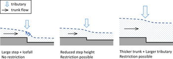
Since MacGregor and others (Reference MacGregor, Anderson, Anderson and Waddington2000) postulate that Q trib/Q trunk > 0.3 likely results in a significant bedrock step, we hypothesise that trunk restriction by a tributary in surge-type glaciers may only occur in situations where subglacial erosion is reduced or where structural controls prevent step formation. Reduced glacial erosive power occurs in cold to polythermal glaciers, slower flowing and small glaciers, in mountain ranges that have been recently glaciated, at low/reverse bed slopes or overdeepenings, and in glacier systems with either very little basal debris or underlain by a till layer of substantial thickness (Hooke, Reference Hooke1991; Alley and others, Reference Alley1997; Flowers and others, Reference Flowers, Roux and Pimentel2011; Jaeger and Koppes, Reference Jaeger and Koppes2016). Several of these are indicative of reduced subglacial drainage, which prevents flushing of sediments necessary to expose bedrock to erosion by ice (Hooke, Reference Hooke1991; Alley and others, Reference Alley1997; Swift and others, Reference Swift, Nienow, Spedding and Hoey2002), and leads to weak subglacial water pressure fluctuations reducing sliding (Iken, Reference Iken1981; Herman and others, Reference Herman, Beaud, Champagnac, Lemieux and Sternai2011). Inefficient subglacial drainage in overdeepenings decreases erosion due to till layer retention and topographic ice flow resistance (Hooke, Reference Hooke1991; Alley and others, Reference Alley1997; Flowers and others, Reference Flowers, Roux and Pimentel2011). Bedrock step formation may therefore also be restricted if a tributary enters at the adverse bed slope part of a trunk overdeepening. We suggest an alternative explanation may hold as well, namely that tectonically active regions with an abundance of normal faulting, weaker bedrock, and high uplift and exhumation rates (Ring and others, Reference Ring, Brandon, Willett and Lister1999; Headley and others, Reference Headley, Hallet, Roe, Waddington and Rignot2012), may produce a till layer protecting underlying bedrock from erosion, providing this occurs while maintaining a regular (low) catchment gradient. Steeper catchments, often associated with tectonically active regions, permit more efficient subglacial drainage and therefore more efficient flushing of eroded sediment (Cook and Swift, Reference Cook and Swift2012).
The specific configurations of dendritic surge-type glacier systems suggested here somewhat support the geological and climatic controls that have long been thought to relate to the non-uniform geographic distribution of surge-type glaciers (Post, Reference Post1969; Clarke and others, Reference Clarke, Schmok, Ommanney and Collins1986; Jiskoot and others, Reference Jiskoot, Luckman and Murray2003; Sevestre and Benn, Reference Sevestre and Benn2015; Crompton and Flowers, Reference Crompton and Flowers2016). Many surge-type glacier clusters occur in tectonically-active mountain ranges undergoing rapid erosion (Post, Reference Post1969; Copland and others, Reference Copland2009), which corroborates that soft deformable beds may be a prerequisite for surging behaviour (Harrison and Post, Reference Harrison and Post2003). However, the geometric and geological configurations may deviate from what we suggest here in dendritic surge-type glaciers with ‘contagious’ surges, where surges of tributaries can be triggered by a surge in the trunk glacier or vice versa (Harrison, Reference Harrison1964; Clarke and others, Reference Clarke, Schmok, Ommanney and Collins1986; Glazovskiy, Reference Glazovskiy and Kotlyakov1996).
6. SUMMARY AND CONCLUSIONS
We presented measurements of complex ice flow and related structural glaciology in a dendritic glacier with multiple icefalls in the Canadian Rockies, with a focus on flow at a tributary-trunk junction. Glacier-wide velocities vary from near zero to 65 m a−1 in the trunk and up to ~175 m a−1 in icefalls. Structural glaciology, surface elevation and ice flow patterns reveal negative gradients in speed and associated compression above the tributary-trunk junction, but nearer the junction the trunk is funnelled and flow increases towards a downstream icefall related to a large bedrock step. In Shackleton Glacier, at this time, the tributary diverts the ice flow in the trunk, and no net outflow restriction takes place. Using our field data to estimate relative fluxes of the tributary and trunk flow units in the order of 0.3–0.6, we conclude that the erosion model by MacGregor and others (Reference MacGregor, Anderson, Anderson and Waddington2000) uses a justifiable approximation of these relative fluxes to calculate the resulting relative normalised heights of the bedrock step and the hanging valley. It is the first time that an extant glacier is used to test such a model, and our observations support the model.
Our findings further suggest that once increased erosion at a tributary-trunk junction has resulted in a significant bedrock step, this step configuration may reduce a tributary's influence on the outflow of the trunk. This inference may be relevant for the understanding of tributary glacier outflow restrictions in surge-type glaciers. Based on our results, and common tributary configurations at surge-type glaciers worldwide, we hypothesise that only in geological and glacial erosive situations that prevent formation of large bedrock steps, may tributary/trunk interactions contribute to surge potential.
Further research into tributary-trunk confluence configurations may advance our understanding of controls on surging and improve models of tributary-trunk glacier surging, which have as yet only included simplified treatments (e.g. Oerlemans and van Pelt, Reference Oerlemans and van Pelt2015). As glaciers around the world continue to shrink, rates of glacier thinning, retreat and fragmentation may change the flow fields around tributary junctions. Thus, understanding the blocking potential of tributaries on their trunks will become increasingly important for predicting glacier run-off and sea-level rise.
ACKNOWLEDGEMENTS
Field assistants of the Shackleton Glacier expeditions are thanked for their hard work, during which Canadian Helicopters and Alpine Helicopters stationed in Golden provided helicopter support. We thank Parks Canada (particularly Darrel Zell) for providing access to Radarsat-2 data through the Government of Canada Allocation, administered by the Canadian Space Agency. Mark Mueller assisted with GIS, Gaëlle Gilson with Matlab, Shawn Bubel advised on surveying equipment and Matt Nolan commented on an early draft. Two anonymous reviewers are thanked for their constructive comments. Research funding was to HJ through an NSERC Discovery Grant and University of Lethbridge Professional Supplement.


 Open access