


Introduction
To inform the public on the avalanche danger in mountainous areas, avalanche forecasters publish an avalanche bulletin on a daily basis in winter. The avalanche danger depends on the stability of the snowpack, the frequency distribution of stability and the expected avalanche size (Techel and others, Reference Techel, Müller and Schweizer2020). The avalanche danger is evaluated for different regions, which have an area of typically 200 km2 in Switzerland (Techel and Schweizer, Reference Techel and Schweizer2017). To assess the avalanche danger, data on snow stratigraphy, e.g. from manually observed snow profiles, and snow instability, e.g. direct observations of avalanches or data from stability tests, are taken into account. As observations are rare, numerical snow cover models can increase spatial and temporal resolution of such data. To this end, snow cover models have to provide the detailed snow stratigraphy and ideally information on snow instability. However, snow cover models are not yet widely integrated into avalanche forecasting (Morin and others, Reference Morin2020), one of the reasons being the lack of providing relevant information on snow instability.
The two most advanced snow cover models are Crocus (Brun and others, Reference Brun, David and Sudul1992; Vionnet and others, Reference Vionnet2012) and SNOWPACK (Bartelt and Lehning, Reference Bartelt and Lehning2002; Lehning and others, Reference Lehning, Bartelt, Brown and Fierz2002). Crocus is part of the French model chain SAFRAN–SURFEX/ISBA-Crocus–MEPRA (S2M; Durand and others, Reference Durand, Giraud, Brun, Merindol and Martin1999; Lafaysse and others, Reference Lafaysse2013). SAFRAN provides the meteorological input for Crocus from observations and numerical weather prediction (NWP) models for massifs with similar meteorological conditions (typically 500 km2; Durand and others, Reference Durand, Giraud and Mérindol1998). Crocus then simulates detailed snow stratigraphy on virtual slopes for different aspects and elevations. Finally, the expert system MEPRA provides the avalanche danger for different regions by evaluating the simulated snow stratigraphy combined with stability indices (Giraud and Navarre, Reference Giraud and Navarre1995).
SNOWPACK can be driven with meteorological data from either automatic weather stations (AWSs) or NWP models (Bellaire and Jamieson, Reference Bellaire and Jamieson2013). SNOWPACK simulates the detailed snow stratigraphy, from which layer properties and stability indices are derived. SNOWPACK can be used as a module of the distributed, 3-D model Alpine3D (Lehning and others, Reference Lehning2006). By providing a DEM and a land-use model, data from AWSs are spatially interpolated to the grid points with MeteoIO (Bavay and Egger, Reference Bavay and Egger2014). Hereby, terrain shading and reflection of shortwave radiation are accounted for (Helbig and others, Reference Helbig, Löwe and Lehning2009). At each grid point, SNOWPACK simulates the snow stratigraphy.
Avalanche release is a fracture mechanical problem (McClung, Reference McClung1981), which starts with a failure and crack formation within a weak layer. Once the crack reaches a critical size, it will rapidly propagate outward (McClung and Schweizer, Reference McClung and Schweizer1999; van Herwijnen and Jamieson, Reference van Herwijnen and Jamieson2005; Gaume and others, Reference Gaume, van Herwijnen, Schweizer, Chambon and Birkeland2015), provided the tensile strength of the slab supports crack propagation (Reuter and Schweizer, Reference Reuter and Schweizer2018). Hence, snow instability is best described by failure initiation and crack propagation (Schweizer and others, Reference Schweizer, Jamieson and Schneebeli2003a, Reference Schweizer, Reuter, van Herwijnen and Gaume2016). Various instability metrics were implemented into SNOWPACK, e.g. the skier stability index related to failure initiation (Föhn, Reference Föhn1987; Jamieson and Johnston, Reference Jamieson and Johnston1998; Monti and others, Reference Monti, Gaume, van Herwijnen and Schweizer2016) and the critical crack length related to crack propagation (Gauthier and Jamieson, Reference Gauthier and Jamieson2008; Gaume and others, Reference Gaume, van Herwijnen, Chambon, Wever and Schweizer2017; Richter and others, Reference Richter, Schweizer, Rotach and van Herwijnen2019). Dry snow instability is assessed in SNOWPACK by selecting a weak layer using the structural stability index (SSI; Schweizer and others, Reference Schweizer, Bellaire, Fierz, Lehning and Pielmeier2006) and evaluating stability indices of this layer. However, interpreting these stability indices is a complex task, in particular since multiple weak layers can contribute to the avalanche danger (e.g. Chalmers and Jamieson, Reference Chalmers and Jamieson2001). Alternatively, Techel and Pielmeier (Reference Techel and Pielmeier2014) proposed a method to objectively evaluate the snowpack structure as a whole.
So far, distributed snow cover modeling was mostly used to simulate the variability of snow depth or snow water equivalent at the scale of an Alpine catchment (Mott and others, Reference Mott, Schirmer and Lehning2011; Schlögl and others, Reference Schlögl, Marty, Bavay and Lehning2016; Wever and others, Reference Wever, Comola, Bavay and Lehning2017) or at the scale of mountain ranges (Quéno and others, Reference Quéno2016; Vionnet and others, Reference Vionnet2016). Very few studies addressed spatial snow instability modeling. For example, SNOWPACK was forced with meteorological data from an NWP model to predict the formation of surface hoar at a regional scale (Bellaire and Jamieson, Reference Bellaire and Jamieson2013; Horton and others, Reference Horton, Schirmer and Jamieson2015). They showed that errors from NWP models affected the formation of critical layers. At a larger scale, Horton and Jamieson (Reference Horton and Jamieson2016) modeled the formation of surface hoar for different locations in Canada using NWP data as input to SNOWPACK. The model slightly overestimated the formation of surface hoar layers and these layers were mostly selected as critical layers right after burial but hardly persisted as critical layers. Vernay and others (Reference Vernay, Lafaysse, Mérindol, Giraud and Morin2015) estimated the uncertainties of forecast avalanche hazard index from NWP models, by combining the French model chain S2M with an ensemble of meteorological predictions. They suggested uncertainties from NWP models to be the main source of uncertainty in the forecast avalanche hazard index. They focused on differences between mountain ranges without considering the spatial distribution of the avalanche hazard index within a region. Furthermore, a comprehensive interpretation of this avalanche hazard index is lacking, since validation of avalanche danger is generally difficult (Schweizer and others, Reference Schweizer, Kronholm and Wiesinger2003b).
At the scale of an alpine basin, Reuter and others (Reference Reuter, Richter and Schweizer2016) modeled spatially distributed snow instability for one weak layer with Alpine3D. To account for preferential deposition, they applied a correction for precipitation based on average wind direction and terrain (Winstral and others, Reference Winstral, Elder and Davis2002). They showed that Alpine3D could not reproduce the variability in snow instability observed in the field and attributed this to too low variations in snow depth. Recently, Bellaire and others (Reference Bellaire, van Herwijnen, Bavay and Schweizer2018) used Alpine3D to investigate the number of critical layers and the percentage of faceted crystals in complex terrain at a regional scale. Variations in snow stratigraphy were small, which was also attributed to small variations in simulated snow depth. Snow depth distribution is very complex in mountainous areas (e.g. Pomeroy and others, Reference Pomeroy1998; Clark and others, Reference Clark2011; Mott and others, Reference Mott, Schirmer and Lehning2011; Bühler and others, Reference Bühler2015; Helbig and van Herwijnen, Reference Helbig and van Herwijnen2017) and can influence physical processes within the snowpack. Indeed, Richter and others (Reference Richter, van Herwijnen, Rotach and Schweizer2020) showed that modeled stability criteria were mostly sensitive to uncertainties in precipitation. To obtain realistic patterns of snow instability, snow cover modeling has to account for realistic precipitation patterns. Such patterns are largely shaped by snow transport by wind, therefore computationally expensive snowdrift modeling is necessary (e.g. Essery and others, Reference Essery, Li and Pomeroy1999; Mott and Lehning, Reference Mott and Lehning2010; Vionnet and others, Reference Vionnet2014; Gerber and others, Reference Gerber2018). Such high-resolution modeling approaches (resolution of a few meters) on large domains are still out of reach for operational use. Therefore, alternative approaches were suggested, which are either based on scaling precipitation input using terrain (e.g. Winstral and others, Reference Winstral, Elder and Davis2002; Helbig and others, Reference Helbig, Mott, van Herwijnen, Winstral and Jonas2017) or measured snow depth data (Vögeli and others, Reference Vögeli, Lehning, Wever and Bavay2016). Nevertheless, higher spatial resolution is needed to reproduce complex snow deposition in alpine terrain, which will affect snow processes (Morin and others, Reference Morin2020).
In this study, we simulated distributed snow instability at a regional scale for the winter season 2016–17 for Davos, Switzerland. We focused, in particular, on the spatial variability of snowpack structure and snow instability. For different weak layers, the temporal evolution and the spatial distribution of snow instability was assessed in terms of the skier stability index and the critical crack length and compared to the forecast avalanche danger level. The overall goal was to investigate whether distributed snow cover modeling can be used to provide information on spatial stability patterns relevant for regional avalanche forecasting.
Methods
Study site and field data
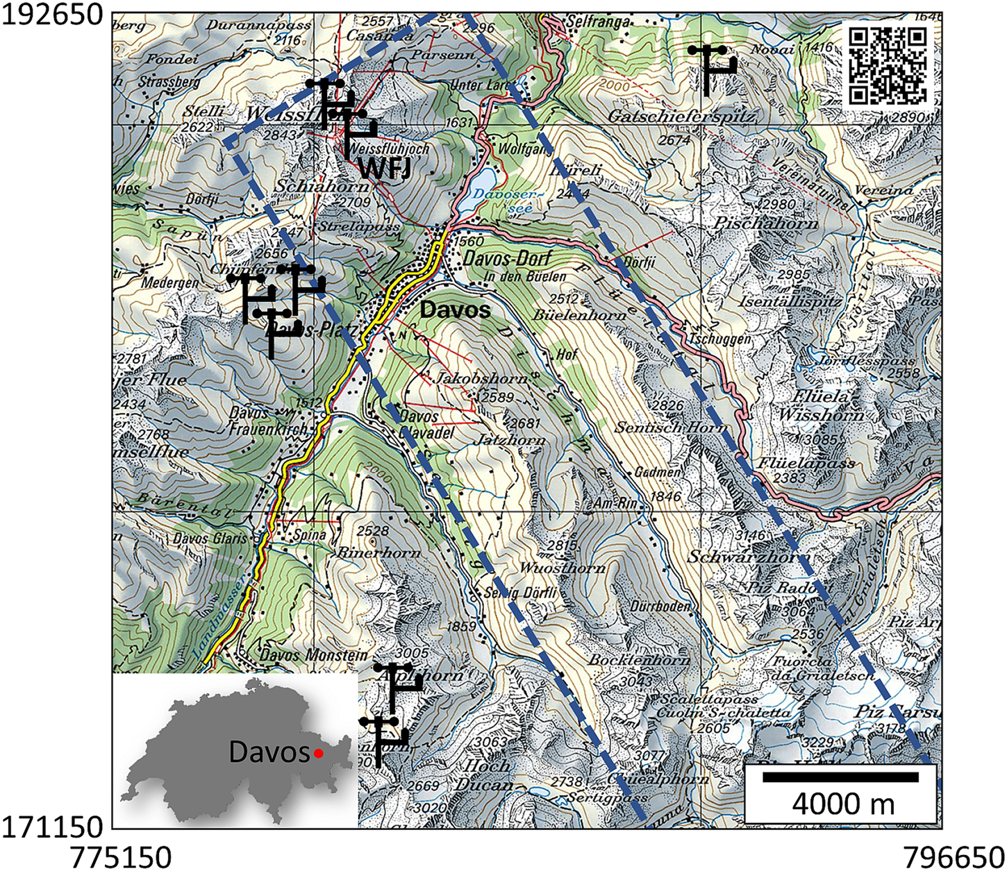
We performed spatial snow cover simulations for the winter season 2016–17 for the region of Davos, Switzerland (Fig. 1). This region covers an area of ~400 km2, which is in the range of the smallest units of the warning regions in Switzerland (Techel and Schweizer, Reference Techel and Schweizer2017). Several AWSs are located around Davos (Fig. 1). These stations belong to the Intercantonal Measurement and Information System (Lehning and others, Reference Lehning, Bartelt and Brown1999), which currently consists of 182 AWS, distributed over the Swiss Alps. These stations provide the necessary input to the snow cover model.
Model domain (21.5 km × 21.5 km) covering the region of Davos, Switzerland. Black icons indicate the locations of the AWSs used for the spatial interpolation of meteorological data. Blue dashed line indicates the approximate area of the airborne laser scan (Section ‘Snow depth data’). Coordinates are in the Swiss coordinate system in m (CH1903). Map from swisstopo (https://s.geo.admin.ch/8963a91333).
Next to the high density of AWS, the region of Davos offered frequent manual snow profile observations, which makes this region ideally suited for this study. At the field site Weissfluhjoch (2536 m a.s.l.) above Davos, Switzerland, manual snow profiles were observed on an almost weekly basis (Richter and others, Reference Richter, Schweizer, Rotach and van Herwijnen2019). For each layer, data on grain type, grain size and hand hardness were recorded according to Fierz and others (Reference Fierz2009). Furthermore, the avalanche warning service, which is located in Davos, monitors an area of 175 km2 around Davos on a daily basis to gather information on the number, size and type (dry or wet-snow) of avalanches. Based on these avalanche observations, we determined an avalanche activity index (AAI) for each day by summing up all recorded avalanches and weighting each avalanche by its size and its triggering type, following the approach used by Schweizer and others (Reference Schweizer, Mitterer, Techel, Stoffel and Reuter2020). Hereby, avalanche sizes were classified to sizes from 1 to 4 and for each class, weights were assigned, which increased by an order of magnitude for each class from 0.01 to 10. The triggering type was considered using weight 1 for natural avalanches, 0.5 for human-triggered avalanches, 0.2 for other artificially triggered avalanches and 0.81 for unknown triggering type. Hence, the AAI is a dimensionless variable.
We also used the forecast avalanche danger level for the region of Davos, based on the European five-degree danger scale (1-Low, 2-Moderate, 3-Considerable, 4-High, 5-Very High) (e.g. Meister, Reference Meister1995). The avalanche danger level is usually attributed to specific aspects and elevations. To qualitatively compare modeled instability and forecast avalanche danger level per aspect, slopes that do not satisfy both criteria (elevation and aspect) were visualized with one level lower than the forecast danger level. We used the corrected danger level, as suggested by Schweizer and others (Reference Schweizer, Mitterer, Techel, Stoffel and Reuter2020). The forecast was corrected in hindsight based on the AAI for this region and after reconsidering meteorological data. On six days of the winter season 2016–17, the avalanche danger was raised one level from 3-Considerable to 4-High.
Snow depth data
To scale the precipitation input for Alpine3D, we used snow depth data obtained from airborne laser scanning (ALS) on 20 March 2017, covering an area of ~140 km2 (Fig. 2a). This dataset, consisting of gridded snow depth data at 3 m spatial resolution, was described in Helbig and others (Reference Helbig2021) and subsets were validated in Mazzotti and others (Reference Mazzotti2019). We eliminated 16% of the grid points, since these were in forests, urban areas and lakes. Snow depth above 8 m (in total ten grid points) were treated as outliers and discarded. In analogy to Kostadinov and others (Reference Kostadinov2019), snow depths below 0.15 m were considered as snow free. To avoid that grid points in Alpine3D were scaled with zero, we eliminated these grid points that were snow free at the time of the laser scan. Finally, we averaged snow depth data to the Alpine3D resolution of 100 m (Fig. 2).
(a) Snow depth data over the valley of Dischma, Switzerland on 20 March 2017 retrieved with ALS and averaged to a resolution of 100 m. The laser scan is centered in the simulation domain and covered an area of ~140 km2. Axes are Swiss coordinate system CH1903 in m. (b) Inset of 3000 m × 3500 m of the simulation domain. Coordinates of the lower left corner are 788′650, 178′550 (CH1903). Grid cells with no data are indicated in white and gridcells exceeding 3 m are indicated in yellow.

Alpine3D
Alpine3D is a 3-D model that couples the snow cover model SNOWPACK with a DEM and a land-use model (Lehning and others, Reference Lehning2006). The simulation domain covered an area of 21.5 km × 21.5 km around Davos, Switzerland (Fig. 1). Elevation ranged from 1255 to 3218 m. Richter and others (Reference Richter, van Herwijnen, Rotach and Schweizer2020) showed that modeled snow instability was mostly sensitive to uncertainties in precipitation. Furthermore, a bias in air temperature of ~1°C influenced the formation of a weak layer, which corresponds to an elevation difference of 100 m under a dry-adiabatic atmosphere. Smaller uncertainties in meteorological input did not influence modeled snow instability. We therefore decided to use a resolution of 100 m, yielding 46 225 grid points. With this resolution, 24% of the grid points had slope angles above 30°. We used in total 13 AWS inside and outside the domain (8 AWS inside the domain; see Fig. 1). Meteorological data from the AWS, such as air temperature (TA), relative humidity (RH), wind velocity (VW), precipitation (P), incoming shortwave radiation (ISWR) and incoming longwave radiation (ILWR) were preprocessed and interpolated to a spatial grid with a 100 m cell resolution (100 m × 100 m) using MeteoIO (Bavay and Egger, Reference Bavay and Egger2014, see details below). At each gridcell, the interpolated meteorological data were used to drive the 1-D model SNOWPACK to simulate snow stratigraphy (Bartelt and Lehning, Reference Bartelt and Lehning2002; Lehning and others, Reference Lehning, Bartelt, Brown and Fierz2002).
Meteorological data were filtered with MeteoIO using standard thresholds, e.g. RH was limited to 5 and 100%. Data gaps shorter than a day were linearly interpolated, data gaps longer than a day were excluded from spatial interpolations. Then, data were spatially interpolated to each gridcell, using interpolation algorithms described in Bavay and Egger (Reference Bavay and Egger2014). TA was interpolated to each grid point with inverse distance weighting using a lapse rate calculated from the AWS. RH was interpolated by first calculating the dew point temperature from TA and RH for each station (Liston and Elder, Reference Liston and Elder2006). Dew point temperature lapse rate was then calculated from the stations and dew point temperature was interpolated with inverse distance weighting. From interpolated TA and dew point temperature, relative humidity was calculated. Wind velocity and incoming long wave radiation were vertically detrended with an elevation lapse rate calculated from the AWS, averaged and then retrended with this lapse rate to each grid point. ISWR was interpolated by accounting for reflection from surrounding terrain using a radiation balance model. Therefore, ISWR was split into direct and diffuse radiation by comparing ISWR with the potential maximum radiation at each time step (Helbig and others, Reference Helbig, Löwe, Mayer and Lehning2010). Then ISWR and the splitting factor were interpolated to each gridcell using inverse distance weighting. Direct radiation was calculated at each grid point, by using the DEM and the solar position at the time step and accounting for terrain shading effects. Terrain reflection at each gridcell was approximated by obtaining a terrain view factor based on a sky-view approach (Anslow and others, Reference Anslow, Hostetler, Bidlake and Clark2008), and multiplying it with the albedo of the gridcell.
A recent sensitivity study highlighted the importance of precipitation on snow instability (Richter and others, Reference Richter, van Herwijnen, Rotach and Schweizer2020). We therefore used an interpolation scheme, which scaled precipitation based on spatial snow depth measurements (see Section ‘Snow depth data’) from ALS. First, precipitation was interpolated to each gridcell with inverse distance weighting using a constant elevation lapse rate derived from AWS. Then we applied the iterative scaling method proposed by Vögeli and others (Reference Vögeli, Lehning, Wever and Bavay2016). The interpolated precipitation was scaled in two steps. First, at each gridcell i where measured snow depth was available, precipitation P i,t was scaled with measured snow depth HS i,obs for each time step t:

Here, P avg,t is the average precipitation in the domain, as derived from the spatial interpolation without scaling and HS avg,obs is the average observed snow depth (Section ‘Snow depth data’). Second, the simulated snow depth data HS i,sim were evaluated on the day of the laser scan (20 March 2017) to obtain a correction factor c = HS i,obs/HS i,sim based on the ratio of observed and simulated snow depth for each grid point. With this, precipitation after the second iteration P 2nd,i,t can be written as:

The correction factor from the second iteration was too high for grid points with HS i,sim < 15 cm at the date of the ALS. We therefore excluded these grid points from scaling with precipitation after the first iteration, to avoid unrealistically high snow depths after the second iteration. Instead, inverse distance weighting was used to interpolate precipitation input for all grid points without scaling parameters. In total, precipitation was scaled for 13 816 grid points.
In the following, we will refer to the simulation without scaled precipitation as basic Alpine3D simulation and to the simulation with scaled precipitation as scaled Alpine3D simulation.
Modeled snow instability metrics
Snow instability of weak layers was assessed using two criteria: the skier stability index SK38 and the critical crack length r c. Both indices were calculated from modeled layer properties. SK38 is the ratio of the shear strength of the weak layer τ p to the shear stress at the depth of the weak layer, calculated for a 38° slope (Jamieson and Johnston, Reference Jamieson and Johnston1998):

Here, τ s is the shear stress acting on the weak layer due to the load of the overlying slab $\tau _{\rm s} = \rho _{sl} g D_{sl} \sin ( 38^\circ ) \cos ( 38^\circ )$ and Δτ is the additional stress due to the skier with ρ sl the density of the slab, g is the acceleration due to gravity and D sl is the slab depth vertically from the snow surface. The skier stress Δτ is modeled as a line load (Föhn, Reference Föhn1987) and simplifies to Δτ = 155/(D sl − P k) mPa (Monti and others, Reference Monti, Gaume, van Herwijnen and Schweizer2016), with P k = 34.6/ρ avg,30 the ski penetration depth and ρ avg,30 is the average density of the upper 30 cm of the snowpack (Schweizer and others, Reference Schweizer, Bellaire, Fierz, Lehning and Pielmeier2006). Modeled shear strength τ p was implemented in SNOWPACK for different grain types and depending on density according to Table 8 in Jamieson and Johnston (Reference Jamieson and Johnston2001). Shear strength of surface hoar was implemented according to Lehning and others (Reference Lehning, Fierz, Brown and Jamieson2004).
The modeled critical crack length r c according to Gaume and others (Reference Gaume, van Herwijnen, Chambon, Wever and Schweizer2017) was only validated with flat field measurements (Richter and others, Reference Richter, Schweizer, Rotach and van Herwijnen2019). Therefore, we extrapolated layer properties to the flat and used those to calculate the critical crack length:

with E′ = E/(1 − ν 2) the plane strain elastic modulus of the slab ν = 0.2 the Poisson's ratio of the slab, and σn = ρ sl gD sl the normal stress acting on the weak layer due to the overlying slab. E is the elastic modulus of the slab, which was related to the slab density by a power law fit (Scapozza, Reference Scapozza2004):

F wl is a correction factor (Richter and others, Reference Richter, Schweizer, Rotach and van Herwijnen2019):

with ρ wl the weak layer density, gs wl the weak layer grain size, ρ ice = 917 kg m−3 the density of ice and gs 0 = 0.00125 m the reference grain size. For both metrics, SK38 and r c, higher values indicate higher stability.
In SNOWPACK, the SSI was used to automatically select the most critical weak layer. The SSI combines SK38 with structural differences D across layer boundaries (Schweizer and others, Reference Schweizer, Bellaire, Fierz, Lehning and Pielmeier2006):

where

Here, ΔR is the difference in hand hardness between two adjacent layers, and Δgs is the difference in grain size. For each modeled layer, the SSI is calculated and the weak layer is then defined as the layer with the lowest SSI and a depth between the penetration depth P k and 100 cm + P k below the snow surface. If differences of SSI between two layers are small (<0.09) but D was smaller for the deeper layer, i.e. structural differences were more prominent, the deeper layer was chosen as the weak layer.
Weak layers
We investigated modeled snow instability for two layers, which were frequently selected with the SSI. These two layers developed at the snow surface during long dry periods (see Section ‘Simulated snow stratigraphy at WFJ’). They are referred to as WL Dec and WL Jan. To identify these weak layers in all simulated profiles, we used the deposition date for each snow layer to determine the boundaries of the potential weak layer. For WL Dec, we considered all layers as potential weak layers that were deposited between 16 November 2016 and 2 January 2017, as in Richter and others (Reference Richter, van Herwijnen, Rotach and Schweizer2020). For WL Jan, we considered all layers deposited between 13 and 30 January 2017. To find a weak layer within these boundaries, we only considered layers consisting of persistent grain types, i.e. depth hoar, surface hoar, facets or rounding facets. Finally, the weak layer was defined as the layer consisting of persistent grains with the lowest value of ρ/gs, with ρ the density of the layer and gs the grain size of the layer. This criterion was chosen since weak layers generally consist of soft (low density) snow with large grains (e.g. Schweizer and Jamieson, Reference Schweizer and Jamieson2001).
Modeled snowpack structure index
To classify the entire snow profile rather than provide stability metrics for specific weak layers, we used the snowpack structure index suggested by Techel and Pielmeier (Reference Techel and Pielmeier2014):

The first term TSAlayer index is the normalized fraction of the snowpack that is soft (hardprop, i.e. percentage of the profile with hand hardness index ≤2), coarse-grained (sizeprop, i.e. percentage of profile with grain size >0.6 mm and hand hardness index ≤3) and faceted (PGprop, i.e. percentage of the profile with persistent grain type). Note that the thresholds mentioned here are those adapted for simulated profiles (Monti and others, Reference Monti, Schweizer and Fierz2014):

The second term TSAmax index is the normalized maximum score TSAmax of the threshold sum at layer interfaces (TSA) (Schweizer and Jamieson, Reference Schweizer and Jamieson2007):

Here, TSA is calculated for each layer interface and increases by one for each criterion which is fulfilled, i.e. grain type is persistent, hand hardness index ≤2, grain size >0.6 mm, difference in grain size ≥0.4 mm, difference in hand hardness index ≥1 and depth of the layer from the snow surface between 18 and 94 cm. Thresholds were again adapted for simulated profiles (Monti and others, Reference Monti, Schweizer and Fierz2014).
The third term slabdepth index is the slab depth D index, which was normalized and restricted to values between 0 and 1, where 1 corresponds to a slab depth of 30 cm or lower and 0 corresponds to a slab depth of 200 cm or larger:

Here, D index is the depth from the snow surface of the uppermost persistent layer with grain size >0.6 mm and hand hardness index ≤2, which is at least 15 cm below the snow surface.
For a more detailed description of the snowpack structure index see Techel and Pielmeier (Reference Techel and Pielmeier2014). SNPKindex ranges from 0 to 3, with 0 indicating very favourable and 3 very unfavourable snowpack structure:

These ranges were defined in Techel and Pielmeier (Reference Techel and Pielmeier2014) and were only evaluated for manually observed snow profiles.
Spatial analysis
Modeled snow stratigraphy data were stored for grid points where the precipitation was also scaled. For these 13 816 grid points, modeled instability metrics were evaluated with a particular focus on the influence of topography, namely aspect Φ and elevation z. The individual grid points were thus grouped in four aspect classes:

where N are north-facing slopes, E are east-facing slopes, S are south-facing slopes and W are west-facing slopes. Grid points were also assigned to elevation bands of 200 m, e.g. 2400 m ≤ z < 2600 m. Grid points that were snow free were excluded. When assessing spatial trends in snow instability metrics, grid cells that did not have a weak layer (see Section ‘Weak layers’) were also excluded.
Results
Winter evolution
The winter 2016–17 started rather late with below-average snow depth in the region of Davos, Switzerland (Fig. 3a). In November 2016, ~50 cm of new snow accumulated at the Weissfluhjoch field site. The snow depth then remained unchanged until the beginning of January 2017. During this period the regional forecast avalanche danger stayed mostly at 1-Low (green in Fig. 3b). In January 2017, snow depth and forecast avalanche danger level increased and avalanches were occasionally observed. On 1 February 2017, with 40 cm of new snow, a first avalanche cycle was observed and in hindsight, the avalanche danger was corrected from 3-Considerable to 4-High (Schweizer and others, Reference Schweizer, Mitterer, Techel, Stoffel and Reuter2020). During a second snow storm in March 2017, many large avalanches released and the avalanche danger level was 4-High. After that avalanche cycle, the avalanche danger level decreased to 1-Low in mid-March 2017. On 49% of the days, the avalanche danger was estimated to be lower on slopes of southern aspect.
(a) Measured snow depth (black line), 80-year mean snow depth (dashed green line) and 80-year minimum snow depth (dashed gray line) at the Weissfluhjoch field site above Davos, Switzerland. Blue bars indicate the AAI for the region of Davos, Switzerland. (b) Forecast avalanche danger level (adjusted by Schweizer and others, Reference Schweizer, Mitterer, Techel, Stoffel and Reuter2020) for different aspects for the region of Davos, Switzerland. Aspects, which were not explicitly mentioned in the forecast were assigned to the next lower danger level. Black striped area indicates the most critical elevation range. Arrows indicate the days 12 February 2017 and 26 March 2017, which are investigated in more detail in Section ‘Snowpack structure index’.

Simulated snow depth distributions
Measured spatial snow depth was highly variable with an average snow depth of 128 cm and a std dev. of 74 cm on 20 March 2017 (Fig. 2a). Convex terrain features (e.g. ridges) accumulated less snow than concave terrain features (e.g. gullies; see Fig. 2b). The basic Alpine3D simulation and the scaled Alpine3D simulation showed clear differences in modeled snow depth (Fig. 4). The basic Alpine3D simulation clearly did not represent the observed spatial variability (orange dots in Fig. 4a). Modeled snow depth for the basic Alpine3D simulation ranged from 16 to 251 cm (mean: 136 cm, std dev.: 85 cm) and the mean relative error was 37%. For the scaled Alpine3D simulation (blue dots in Fig. 4a), the mean relative error was reduced to 17% (mean: 134 cm, std dev.: 45 cm) and the simulated snow depths were much closer to the observations across the entire range. In the following, we focused on snow stability for the scaled Alpine3D simulations.
(a) Modeled snow depth obtained with Alpine3D compared to measured snow depth from ALS on 20 March 2017. Blue dots show the scaled Alpine3D simulation and orange dots the basic Alpine3D simulation. Modeled snow depth for (b) the scaled Alpine3D simulation and (c) the basic Alpine3D simulation for the same section as shown in detail in Figure 2b. Gridcells with no data are indicated in white and grid cells exceeding 3 m are indicated in yellow.

Simulated snow stratigraphy at WFJ
At the Weissfluhjoch field site the manual snow profile on 1 January 2017 showed that most of the snowpack consisted of depth hoar (dark blue in Fig. 5a). These snow layers formed a weak base that persisted throughout the entire season and was consistently observed in manual snow profiles in the lower 40 cm of the snowpack. On top of this layer, rather harder layers existed consisting of smaller faceted crystals and rounded grains. On 24 January 2017, surface hoar developed at the snow surface and was buried on 1 February 2017. Subsequently, this layer of buried surface hoar was observed in most manual profiles at a depth of ~80 cm until 1 March 2017.
(a) Manually observed snow profiles at the Weissfluhjoch field site for the winter season 2016–17. (b) Evolution of modeled grain type for the corresponding Alpine3D grid point for the scaled Alpine3D simulation. The black line indicates the automatically selected layer using the SSI. (c) Modeled SK38 and (d) modeled r c of the (black) automatically selected layer, (blue) WL Dec and (pink) WL Jan.

In Alpine3D, the grid point for Weissfluhjoch had an elevation of 2539 m and a slope angle of 11°. Modeled snow stratigraphy at this grid point resembled observed stratigraphy well (Fig. 5b). The base of the snowpack consisted mostly of depth hoar, in particular at a depth of 30–50 cm (WL Dec). Snow layers above 50 cm mostly consisted of faceted crystals and rounded grains. On 1 February 2017, a layer of surface hoar at a snow height of ~100 cm (WL Jan) was buried in the simulations, in line with the observations.
Over the course of the winter season, r c values gradually increased for both weak layers. The increase was more rapid for WL Jan, and values of r c were generally lower for WL Dec than for WL Jan (blue and pink lines in Fig. 5d). For SK38, on the other hand, WL Dec initially had higher values than WL Jan, while the opposite was true from March 2017 on (blue and pink lines in Fig. 5c). In the first half of February 2017, the instability metrics for WL Jan, and in particular SK38, changed rapidly (pink lines in Figs 5c, d). This was an artifact of the method used to define weak layers. The layers considered for WL Jan were the layers located close to the snow surface at the end of January 2017: a layer of surface hoar on top of a layer consisting of depth hoar crystals. For WL Jan, the layer with the lowest value of ρ/gs was chosen. Up to 14 February 2017, this was the surface hoar layer, while afterward WL Jan corresponded to the depth hoar layer. Accordingly, on 14 February, there was a sudden decrease in SK38 for WL Jan, and a more modest decrease in r c.
Between 1 November 2016 and 1 May 2017, WL Dec was automatically selected with the SSI on 16% of the days as most critical layer, mostly in January and February (black dashed line in Fig. 5b). After 1 March 2017, WL Dec was not selected anymore as it was $\gtrsim$ 100 cm below the snow surface. From 1 February 2017 to 1 May 2017, WL Jan was selected with the SSI as the most critical weak layer on 68% of the days. Jumps in stability indices for the layer automatically selected with the SSI correspond to sudden changes in the selected layer. In the first week of February, for instance, the automatically selected layer using the SSI jumped to the old snow surface at a snow depth of ~100 cm, i.e. the location of WL Jan (black dashed line in Fig. 5b). Although the automatically selected layer coincided with WL Jan, stability metrics were different (black and pink line in Figs 5c, d). This was again an artifact of the different weak layer picking methods. For the automatic method relying on the SSI, the structural difference D was taken into account (see Eqn (8)). For both, the surface hoar and depth hoar layer, differences in grain size were large, resulting in D = 1 for both layers. Hence, the layer with the lower shear strength was selected, which in our simulation was the layer of depth hoar.
Simulated snow stratigraphy on north- and south-facing slopes
The Weissfluhjoch is a flat field site. To highlight differences between aspect at roughly the same elevation, Figure 6 shows the snow stratigraphy for a north- and a south-facing grid point at an elevation of ~2500 m a.s.l. (Fig. 6). Generally, the snow stratigraphy at the north-facing grid point (Fig. 6a) looked fairly similar to the simulated snow stratigraphy at the Weissfluhjoch gridcell (Fig. 5), whereas the stratigraphy at south-facing grid point showed pronounced differences. The snow cover of the south-facing grid point consisted of more melt forms (red colors in Fig. 6) than the north-facing grid point. By mid-March 2017, the south-facing snowpack completely consisted of melt forms, as melt water had infiltrated the snow cover. On the north-facing grid point, on the other hand, the snowpack was still completely dry on 1 May 2017 (end of simulation period). WL Dec and WL Jan, which were investigated in more detail, were both selected with the SSI for distinct periods at both grid points (black line in Fig. 6a, b). More precisely, WL Dec was selected on one-third of the days between 1 November 2016 and 1 May 2017 (38% N, 31% S), while WL Jan was selected on around one fifth of the days (12% N, 20% S). On the north-facing grid point, WL Jan consisted first of surface hoar, which disappeared after 21 February 2017, and then of faceted crystals. On the south-facing grid point, the snow surface in January transformed into a thick layer (~6 cm) of depth hoar which formed WL Jan.
Evolution of modeled grain type for (a) a north-facing grid point and (b) a south-facing grid point for the scaled Alpine3D simulation. Both grid points had an elevation of ~2500 m a.s.l. and a slope angle of 30° and 35°. For both grid points, the snow depth was average (i.e. ±20%) within the elevation band of 2400 to 2600 m and the range of slope angles (30–40°). Black lines indicate the automatically selected layer using the SSI. (c) Modeled SK38 and (d) modeled r c of (blue) WL Dec and (pink) WL Jan.

There were substantial differences in SK38 and r c over the season for the north- and the south-facing grid points. From January 2017 until mid-March 2017, r c values for WL Dec and WL Jan were very similar for both aspects (Fig. 6d). However, SK38 showed some differences: for WL Dec, SK38 was lower for the north-facing slope than for the south-facing slope (Fig. 6c). In contrast, for WL Jan, SK38 was lower for the south-facing slope than for the north-facing slope. In mid-March 2017 when the snowpack at the south-facing grid point transformed into melt forms, both instability metrics rapidly increased for the south-facing slope.
Evolution of snow instability metrics for WL Dec and WL Jan
In the following, we show the evolution of modeled snow instability metrics for the scaled Alpine3D simulation for WL Dec and WL Jan over the entire model domain. The median value of SK38 increased from initially ~0.4–1.0 in the beginning of March 2017 for both weak layers (Fig. 7a). Around 9 March 2017, SK38 briefly decreased after which it increased more or less steadily. Generally, the increase in SK38 was more rapid for WL Jan than for WL Dec over the entire simulation period. In February 2017, SK38 for WL Jan was lower than for WL Dec while after 1 March 2017, SK38 for WL Jan was higher than for WL Dec. The interquartile range (IQR; shaded areas in Fig. 7) for WL Dec remained rather narrow and constant until mid-March 2017. For WL Jan, on the other hand, the IQR was initially very large, indicating that SK38 for this weak layer was more variable in the terrain. The IQR for WL Jan decreased, until it reached a minimum in the middle of March 2017. After mid-March, the IQR increased rapidly for both layers, while WL Dec lagged a few days behind WL Jan.
(a) Median SK38 values and (b) median r c values for WL Dec (blue line) and WL Jan (pink dashed line) with time. Line represents the median of all 13 816 grid points for the scaled Alpine3D simulation. Shaded areas show the IQR of the simulations.

Differences in critical crack length were less pronounced for both layers. The median of r c was similar for both layers and slightly increased. After 10 March 2017, r c for WL Jan increased more rapidly than for WL Dec. Compared to SK38, the IQR for r c was smaller. The IQR of r c increased with time, while showing similar variability for both layers.
To investigate the spatial variation of instability metrics, we analyzed the dependency on aspect for both layers (Fig. 8). For WL Dec, instability metrics did not show much difference with aspect (Figs 8a, c). SK38 was slightly lower on north- and east-facing grid points during the entire season. For r c no clear aspect dependence was observed in the winter months. End of March 2017, instability metrics on south- and west-facing slopes rapidly increased. For WL Jan, both indices were lower on south-facing grid points than on north-facing grid point in winter (Figs 8b, d). By mid-March 2017, median SK38 and r c values rapidly increased for south- and west-facing grid points, while on east- and north-facing grid points, SK38 and r c only gradually increased up to the end of the simulation period.
(a, b) Median SK38 and (c, d) median r c values with time for (a, c) WL Dec and (b, d) WL Jan. Colors indicate the different aspects: (black solid) north (N), (blue dashed) east (E), (pink dotted) south (S) and (cyan dash-dotted) west (W).

The regional forecast avalanche danger level was generally higher for north- than for south-facing slopes during the entire winter season (Fig. 3), in contrast to the simulation results. However, since here we only investigated two specific weak layers, a direct comparison with the avalanche danger level is not straightforward. To interpret the entire snowpack, without focusing on specific weak layers, in the following we present the results for the snowpack structure index.
Snowpack structure index
The bi-weekly distributions of SNPKindex for the scaled Alpine3D simulation showed that initially (until 12 March 2017) north- and south-facing grid points were similar (blue to yellow lines in Fig. 9). Most grid points had high values for SNPKindex and the mode was located in the category ‘very unfavorable’. Except for two dates (15 January 2017 and 29 January 2017), distributions were narrower for north-facing slopes (Fig. 9a), indicating less variability for north-facing grid points. After 26 March 2017, the distributions showed clear differences. Distributions for north-facing grid points flattened although the mode was still ‘very unfavorable’. In contrast, south-facing grid points clearly had a bimodal distribution (Fig. 9b), with a second mode located at lower values for SNPKindex.
Bi-weekly probability density functions of the snowpack structure index (SNPKindex) from 1 January 2017 to 23 April 2017 for (a) all north-facing slopes and (b) south-facing slopes for the scaled Alpine3D simulation. The black line indicates the threshold above which a snowpack is classified as ‘very unfavorable’ (see Eqn (13)).

For 2 d shown in Figure 9, we visualized the snowpack structure index in more detail with respect to aspect and elevation (Fig. 10). The first day was 12 February 2017 when both probability density functions were similar (compare light blue lines in Fig. 9). The second day was 26 March 2017, when south-facing grid points had a bimodal distribution, while north-facing grid points were still unimodal (compare orange lines in Fig. 9). On 12 February 2017, the regional danger level was 3-Considerable above 2000 m a.s.l. On 26 March 2017, the regional danger level was 2-Moderate above 2400 m a.s.l. For both days, the avalanche warning service estimated that south-facing slopes were more stable (see arrows in Fig. 3). The spatial pattern of the percentage of grid points classified as ‘very unfavorable’ (i.e. SNPKindex > 2.5) was very different (Fig. 10). On 12 February 2017, for elevations from 2200 to 3000 m a.s.l., the percentage of grid points classified as ‘very unfavorable’ was higher for south- than for north-facing slopes, especially for higher elevations. This distribution was in contrast to the regional forecast, where the north-facing slopes were estimated to be more critical than the south-facing slopes.
Percentage of grid points classified as ‘very unfavorable’ (i.e. SNPKindex > 2.5) with elevation and aspects for (a) 12 February 2017 and (b) 26 March 2017. The number in each box indicates the number of grid points.

On 26 March 2017, on the other hand, the snowpack structure index was lower, especially for lower elevations and southern aspects. Fewer grid points were classified as ‘very unfavorable’. For elevations below 2000 m a.s.l., the percentage of the grid points classified as ‘very unfavorable’ was 0% for all aspects (purple colors in Fig. 10b). Between 2000 and 3000 m a.s.l., there was a clear difference between aspects as relatively few slopes on southern aspects were classified as ‘very unfavorable’ compared to northern aspects. Above 2400 m a.s.l., the percentage of north-facing grid points classified as ‘very unfavorable’ was very similar to 12 February 2017, suggesting that the snowpack did not evolve much. Above an elevation of 3000 m a.s.l., the percentage of ‘very unfavorable’ grid points was similar for both dates and all aspects. The simulation on 26 March 2017 was in line with the avalanche forecast, where the snowpack on south-facing slopes was estimated to be more stable than on north-facing slopes.
Variations with modeled snow depth
Since highly resolved data of measured snow depths were used to force the scaled Alpine3D simulation, we analyzed how these variations in snow depth influenced modeled stability and snowpack structure metrics for one day. On 12 February 2017, modeled average snow depth above 2000 m was 112 cm. For snow depths up to ~150 cm, the SNPKindex was rather high and mostly classified ‘very unfavorable’ (Fig. 11a). For snow depth above 150 cm, SNPKindex decreased with increasing snow depth for all aspects. Similar behavior was observed for the instability metrics of WL Dec. With increasing snow depth, r c increased for all aspects (Fig. 11c). Also SK38 increased with increasing snow depths up to ~1 m (Fig. 11b). However, for larger snow depths SK38 decreased.
(a) SNPKindex, (b) SK38 of WL Dec and (c) r c of WL Dec with modeled snow depth on 12 February 2017 for all grid points above 2000 m a.s.l. Colors indicate different aspects: (black) north (N), (blue) east (E), (pink) south (S) and (cyan) west (W).

Discussion
To investigate the spatial distribution of snow instability, we used the model Alpine3D to perform distributed snow cover simulations for the region of Davos, Switzerland. We focused on the winter season 2016–17, which was marked by below-average snow depth and prolonged dry periods (Fig. 3). This favored the formation of persistent weak layers at the base of the snowpack. Our results show that SNOWPACK was able to appropriately model this weak base (Fig. 5). Modeled snowpack structure was rather unfavorable the entire winter season throughout the model domain.
Since modeled snow instability is most sensitive to precipitation (Richter and others, Reference Richter, van Herwijnen, Rotach and Schweizer2020), a prerequisite to realistically model spatial snow instability patterns was to correctly represent the snow distribution in mountainous terrain, which is notoriously complex (e.g. Deems and others, Reference Deems, Fassnacht and Elder2008; Shaw and others, Reference Shaw, Gascoin, Mendoza, Pellicciotti and McPhee2020). Different methods have been developed to account for this, from highly resolved snow drift modeling (e.g. Gerber and others, Reference Gerber2018; Mott and Lehning, Reference Mott and Lehning2010; Vionnet and others, Reference Vionnet2014), to rather simple parameterizations (e.g. Winstral and others, Reference Winstral, Elder and Davis2002; Vögeli and others, Reference Vögeli, Lehning, Wever and Bavay2016; Helbig and others, Reference Helbig, Mott, van Herwijnen, Winstral and Jonas2017). Snow drift modeling was not feasible for our application, since it is computationally expensive and high-resolution wind fields were not available. Therefore, we chose to scale precipitation with measured snow depths as suggested by Vögeli and others (Reference Vögeli, Lehning, Wever and Bavay2016). Although the observed snow depth distribution was well reproduced (Fig. 4), this approach does not account for all processes shaping the snow cover. Indeed, only precipitation was scaled with a constant factor for each gridcell, which was obtained from an airborne laser scan on 20 March 2017. Hence, we assumed that the spatial variations were the same during the entire winter and variations in snow properties due to other physical processes, in particular the mechanical altering of snow properties due to wind, were thus not accounted for. As such, the spatial variations of our snow cover simulations are likely less pronounced than in reality. Nevertheless, our results showed variations in modeled snow instability related to elevation, aspect and snow depth, the main drivers generally linked to snow instability (e.g. Reuter and others, Reference Reuter, van Herwijnen, Veitinger and Schweizer2015b).
We investigated two distinct weak layers, WL Dec and WL Jan, which were frequently selected with the SSI method as the most critical layer (Figs 5, 6). The SSI method only took into account layers in the upper 100 cm plus penetration depth of the snowpack (Schweizer and others, Reference Schweizer, Bellaire, Fierz, Lehning and Pielmeier2006), as weak layers below that depth are generally not prone to skier triggering (Schweizer and Jamieson, Reference Schweizer and Jamieson2001; van Herwijnen and Jamieson, Reference van Herwijnen and Jamieson2007). As such, WL Dec was not selected anymore with the SSI if the snow depth was $\gtrsim$ 100 cm. To interpret Alpine3D simulations in terms of snow instability, we analyzed two instability metrics, SK38 and r c of these two weak layers. So far, no robust thresholds for instability exist. Hence, we rather looked at spatial and temporal trends of these instability metrics. Our results showed that immediately after WL Jan was buried, instability metrics were lower for WL Jan, which was closer to the snow surface than for WL Dec (Fig. 7). However, modeled instability metrics for WL Jan increased faster, such that by early March instability metrics were lower for WL Dec (Fig. 7). Hence, modeled instability metrics indicated higher stability for WL Jan than WL Dec by early March, although WL Jan was closer to the snow surface. For the region of Davos, there were two distinct avalanche cycles, one on 1 February 2017 and around 9 March 2017 (Fig. 3). Unfortunately, no fracture line profiles were available, such that the failure layer remained unknown. Our results can be interpreted to mean that avalanches on 1 February 2017 released in WL Jan, while in early March 2017 avalanches released or stepped down to WL Dec. Although weak layers closer to the snow surface are generally more prone to skier triggering, larger snowfalls, as on 9 March 2017, can cause failure in persistent weak layers which are buried more deeply. Indeed, Conlan and others (Reference Conlan, Tracz and Jamieson2014) showed that failures still occurred up to 5 months after burial of a weak layer. Snow cover models could help assess the stability of deep weak layers.
As the frequency distribution of triggering spots is one of the key parameters for assessing the avalanche danger (Techel and others, Reference Techel, Müller and Schweizer2020), we investigated the spatial variability of instability metrics of the two weak layers. Our results suggested that the variability in snow instability metrics was larger for WL Jan (Fig. 7). Modeled snow instability metrics increased more quickly on south-facing slopes in spring, suggesting higher stability on south-facing slopes than on north-facing slopes in spring, in line with the avalanche forecast (Fig. 8). This is a direct consequence of the snowpack structure switching from dry snow to melt forms earlier on south-facing slopes (Fig. 8). However, differences between north- and south-facing slopes were not very pronounced in winter (January to March), and snow instability metrics were actually somewhat lower for one weak layer (WL Jan) on south-facing slopes (Fig. 8). Furthermore, the snowpack structure index indicated more often unfavorable conditions on south-facing slopes (Fig. 10a). Snow instability metrics for WL Jan were likely more unfavorable on south-facing slopes because the simulations predicted more developed faceting on this aspect (Fig. 8). Results were similar when only taking into account slope angles above 30° (not shown). Steep south-facing slopes stabilized slightly before west-facing slopes in spring but also showed lower stability during the winter months. Similar results in terms of number of critical layers or the percentage of faceted crystals were also reported by Bellaire and others (Reference Bellaire, van Herwijnen, Bavay and Schweizer2018). In contrast, the forecast avalanche danger level suggested that south-facing slopes were generally more stable (Fig. 3) during the entire winter. One possible reason for this discrepancy could be that numerous processes are considered in regional avalanche forecasting, including snow drifting, a process that was not explicitly accounted for in our simulations.
In general, based on data from skier-triggered avalanches, it is often assumed that north-facing slopes are less stable than south-facing slopes (e.g. Grímsdóttir and McClung, Reference Grímsdóttir and McClung2006; Schweizer and Jamieson, Reference Schweizer and Jamieson2001). However, various field studies have also shown that this is not always the case. Indeed, Campbell and Jamieson (Reference Campbell and Jamieson2007) reported stability test results from a site where north-facing slopes were more stable than east-facing slopes. They attributed this to larger faceting on east-oriented slopes. Also, Reuter and others (Reference Reuter, Richter and Schweizer2016) reported days on which south-facing slopes were less stable than north-facing slopes. At a much larger scale, a detailed analysis of a wide-spread avalanche cycle in the Swiss Alps in January 2018 from satellite images showed that there were more avalanches on south-facing slopes, excluding glide- and wet-snow avalanches (Bründl and others, Reference Bründl and Steffen2019; Bühler and others, Reference Bühler, Hafner, Zweifel, Zesiger and Heisig2019). Our model results suggest that differences in snow instability between north- and south-facing slopes were low for persistent weak layers during winter months. However, to draw a firm conclusion on model performance, further investigations are required, including different years with different weak layers. A comprehensive assessment of the influence of aspect on snow instability will require numerous stability tests (e.g. Reuter and others, Reference Reuter, Richter and Schweizer2016), fracture line profiles and concurrent profiles on south- and north-facing slopes to help validate model results and increase our understanding of the causes of spatial variability of snow instability. Furthermore, a combination of different instability metrics still has to be linked with observed snow instability, e.g. the avalanche activity. To this end, threshold values have to be defined for modeled snow instability metrics.
Our results highlighted some limitations of the instability metrics. First, SK38 was calculated for a 38° slope while r c was calculated for a flat field. This inconsistency might seem counter-intuitive, as in many avalanche statistics the median slope was found to be close to 38° (e.g. Perla, Reference Perla1977; Schweizer and Jamieson, Reference Schweizer and Jamieson2001). However, when the shear stress due to the overlying slab exceeds the modeled weak layer shear strength, which is typically the case for thicker slabs (Fig. 11b), the r c parameterization for the slope suggested by Gaume and others (Reference Gaume, van Herwijnen, Chambon, Wever and Schweizer2017) and improved by Richter and others (Reference Richter, Schweizer, Rotach and van Herwijnen2019) resulted in negative values of r c. Since r c was only validated for flat field sites (Richter and others, Reference Richter, Schweizer, Rotach and van Herwijnen2019), we deemed it most reasonable to calculate r c for the flat field. Second, some well-known counter-intuitive trends were observed in SK38. Indeed, SK38 initially increases with increasing snow depth due to the decreasing skier stress (Jamieson and Johnston, Reference Jamieson and Johnston1998), suggesting that skier-triggering is less likely for thicker slabs (Fig. 11b). However, for snow depths above one meter, SK38 decreases with increasing snow depth, suggesting skier-triggering is more likely again. For thicker slabs, however, increases in shear strength are less pronounced than increases in the shear stress (Richter and others, Reference Richter, van Herwijnen, Rotach and Schweizer2020), forcing SK38 to decrease. The observed variability in SK38 was thus mostly related to differences in snow depth, in particular later in the season, as the persistent weak layers were buried more deeply. Some studies have excluded the stress exerted by the slab weight from the stability index, to ensure an overall increase in stability index with increasing slab thickness (Reuter and others, Reference Reuter, Schweizer and van Herwijnen2015a; Schweizer and Reuter, Reference Schweizer and Reuter2015).
To obtain a more complete picture of the snowpack, we also investigated the snowpack structure index SNPKindex introduced by Techel and Pielmeier (Reference Techel and Pielmeier2014). According to their classification derived from manually observed profiles north-facing and south-facing slopes generally had an ‘unfavorable’ snow structure (Fig. 9). Yet, the variability was higher for south-facing slopes, yielding more grid points classified as ‘favorable’ and in addition more grid points classified as ‘very unfavorable’ on 12 February 2017 (Fig. 10a). In spring, the number of grid points classified as ‘favorable’ increased for lower elevations (below 2200 m a.s.l.) and south-facing slopes (Fig. 10b), in line with the avalanche forecast. SNPKindex consists of three parts: (1) a structural index combining the percentage of faceted crystals, soft layers and coarse grains, (2) an index describing the structure of the weakest layer using layer interfaces and (3) an index describing slab depth. During a snowfall, the structural index and the slab depth index both decrease causing SNPKindex to decrease and suggesting a more favorable snowpack. Therefore, SNPKindex decreased during precipitation events and hence did not correlate with avalanche activity (not shown). The snowpack structure index was introduced to separately classify snowpack stability and snowpack structure (Techel and Pielmeier, Reference Techel and Pielmeier2014), and hence was not supposed to directly relate to snow instability. However, SNPKindex could provide valuable information prior to precipitation events, as it generally identified the poor snowpack structure that was present in our study area. Combining SNPKindex with forecast meteorological data could be interesting to support avalanche danger assessment.
We used high-resolution snow depth measurements from ALS to scale precipitation throughout our model domain. We only used one single scan from 20 March 2017 for scaling precipitation for the whole winter season. Although we do not know whether the spatial snow depth distribution is representative for the whole winter season, the resulting patterns seem realistic (Fig. 4). Moreover, Schirmer and others (Reference Schirmer, Wirz, Clifton and Lehning2011) reported high intra-seasonal consistency in spatial snow depth distribution for another basin near Davos. Validating the spatial distribution of snow instability, on the other hand, was not possible due to a lack of spatial snow cover observations. However, Richter and others (Reference Richter, Schweizer, Rotach and van Herwijnen2019) thoroughly validated the temporal evolution of the critical crack length and showed that modeled r c values compared well with field observations at the WFJ field site for 2017, which is part of our domain. Comparing our results to a model setup with less complexity, where precipitation was not scaled, the differences in the distribution of the snowpack structure index were not very substantial (not shown). The scaled Alpine3D simulation produced slightly more variability in simulated snowpack structure, however the distribution of SNPKindex was very similar. This suggests that virtual slope simulations (e.g. Durand and others, Reference Durand, Giraud, Brun, Merindol and Martin1999; Lafaysse and others, Reference Lafaysse2013; Horton and others, Reference Horton, Nowak and Haegeli2018) might be sufficient, especially when these are coupled with an ensemble of meteorological input (e.g. Vernay and others, Reference Vernay, Lafaysse, Mérindol, Giraud and Morin2015). However, since we only focused on one specific winter in one specific geographical location, further investigations on different years, e.g. above-average winters, and different locations are required as these might influence model performance (Essery and others, Reference Essery, Morin, Lejeune and Bauduin-Ménard2013; Krinner and others, Reference Krinner2018). Although it is clear that spatial modeling of snow instability could greatly improve avalanche forecasting, our results highlight that more validation data are required – in particular to support or discard some of our counter-intuitive model results.
Conclusion and outlook
We simulated spatially distributed snow instability with Alpine3D for the winter season 2016–17. The model domain covered an area of 21.5 km × 21.5 km around Davos, Switzerland with a spatial resolution of 100 m. Alpine3D was forced with interpolated meteorological data from AWSs. To account for spatial variability from complex snow distribution patterns, precipitation was scaled with high-resolution snow depth measurements from ALS, which was available for around one-third of the simulation domain. Modeled snow instability metrics were assessed for two prominent persistent weak layers and the overall snowpack structure was investigated for almost 14 000 grid points.
The winter season 2016–17 was marked by below-average snow depths and prominent persistent weak layers at the base of the snowpack. Our results showed that SNOWPACK was able to model these weak layers, and we investigated their spatial distribution. Overall, our model results suggested that the snowpack structure and instability metrics were more favorable on south-facing slopes in spring, in line with the forecast avalanche danger level. However, during the winter, model results did not show a clear aspect dependency, and the snowpack on south-facing slopes was even somewhat less favorable, in contrast to the avalanche forecast. However, due to a lack of field data, a comprehensive validation of our results with respect to aspect and elevation was not possible. Therefore, more field data are required to validate spatial patterns of modeled snow instability for different winter seasons. In particular, a comprehensive dataset of snow profile observations and stability tests, combined with snow cover simulations on various aspects are required. Although snow cover simulations are not yet fully integrated in avalanche forecasts, this study is a promising step toward an operational use and our results provide guidance on how to integrate models into operational forecasting.
Acknowledgments
The authors thank Stephanie Mayer for intensive discussions on interpolating meteorological data and interpreting stability indices, Nora Helbig for snow depth data and discussions on Alpine3D interpolation algorithms and Felix von Rütte for the help with validating interpolation algorithms in Alpine3D. We also appreciate the efforts of Janic Cathomen and Pascal Hagenmuller, although their contributions finally did not make it into this manuscript. Furthermore, we thank two anonymous referees and the editor Nicolas Eckert, who helped us to improve this paper. Bettina Richter has been supported by a grant of the Swiss National Science Foundation (200021_169641).


 Open access