


Introduction
The flow of water through glaciers plays a key role in ice dynamics, influencing processes such as basal sliding, internal deformation and subglacial sediment deformation (Hart and others, Reference Hart, Rose, Clayton and Martinez2015). Meltwater storage and movement within the ice also drive transient glacier accelerations, surging behavior and outburst floods (Fountain and others, Reference Fountain, Jacobel, Schlichting and Jansson2005; Harper and others, Reference Harper, Bradford, Humphrey and Meierbachtol2010). The latter, among other glacier hazards, are expected to become more frequent under a warming climate (Clague and O’Connor, Reference Clague, O’Connor, Haeberli and Whiteman2021). To better comprehend the associated risks and the overall response of the interplay between glacier dynamics and hydrology to atmospheric warming, it is vital to understand how water is transported through the ice.
Water is largely supplied to the glacial hydrological system through the surface melting of ice and snow. Supraglacial streams form in the ablation zone and enter the glacier through moulins, near-vertical passageways into the englacial environment that typically initiate where streams intersect crevasses (Holmlund, Reference Holmlund1988). The formation and evolution of englacial drainage systems have been attributed to a variety of mechanisms, including the propagation of fractures driven by hydraulic pressure (Boon and Sharp, Reference Boon and Sharp2003; Alley and others, Reference Alley, Dupont, Parizek and Anandakrishnan2005; van der Veen, Reference van der Veen2007), cut-and-closure processes within incised channels (Fountain and Walder, Reference Fountain and Walder1998; Gulley and others, Reference Gulley, Benn, Müller and Luckman2009a) and the exploitation of existing weaknesses such as debris-laden crevasse traces (Stenborg, Reference Stenborg1969, Reference Stenborg1973; Fountain and others, Reference Fountain, Jacobel, Schlichting and Jansson2005; Gulley and Benn, Reference Gulley and Benn2007). As suggested by Gulley and others (Reference Gulley, Benn, Screaton and Martin2009b), individual englacial drainage pathways are likely to arise through a combination of these processes.
Once water reaches the glacier bed, it is routed toward the glacier terminus via the subglacial drainage system, which can range from inefficient, distributed networks to efficient, channelized systems (Fountain and Walder, Reference Fountain and Walder1998; Schoof, Reference Schoof2010; Flowers, Reference Flowers2015). Distributed drainage consists of widespread, tortuous pathways such as linked cavities or thin water films that maintain high basal water pressures and promote sliding, whereas channelized drainage transports water through discrete conduits that reduce basal water pressure and sliding velocities. As the melt season progresses and the water supply increases, the subglacial drainage system often transitions from a distributed to a channelized configuration capable of rapidly evacuating water (Hewitt, Reference Hewitt2013; Werder and others, Reference Werder, Hewitt, Schoof and Flowers2013; Flowers, Reference Flowers2015). However, transient water pulses from events such as lake drainages or intense rainfall can temporarily overwhelm subglacial drainage networks, causing short-lived increases in basal water pressure and sliding, even within an otherwise efficient channelized system (Iken and Truffer, Reference Iken and Truffer1997; Bartholomew and others, Reference Bartholomew, Nienow, Mair, Hubbard, King and Sole2010).
Current understanding of englacial and subglacial drainage processes has been shaped by a wide array of field observations and modeling efforts (e.g., Werder and others, Reference Werder, Hewitt, Schoof and Flowers2013; Flowers, Reference Flowers2015). However, as the interior and base of glaciers are difficult to access, the observational record is limited in spatial extent, resolution and temporal coverage. Valuable point-scale data have come from borehole studies (e.g., Hodge, Reference Hodge1976; Hubbard and others, Reference Hubbard, Sharp, Willis, Nielsen and Smart1995; Flowers and Clarke, Reference Flowers and Clarke2002b; Fountain and others, Reference Fountain, Jacobel, Schlichting and Jansson2005; Rada Giacaman and Schoof, Reference Rada Giacaman and Schoof2023), moulin-based measurements (e.g., Iken, Reference Iken1972) and from rare excavated tunnels with direct access to the glacier base (e.g., Vivian and Bocquet, Reference Vivian and Bocquet1973; Boulton and others, Reference Boulton, Morris, Armstrong and Thomas1979; Hagen and others, Reference Hagen, Liestøl, Sollid, Wold and Østrem1993; Lappegard and others, Reference Lappegard, Kohler, Jackson and Hagen2006; Lefeuvre and others, Reference Lefeuvre, Jackson, Lappegard and Hagen2015). Dye tracing experiments have offered insight into larger-scale hydrological connectivity and transport efficiency (e.g., Nienow and others, Reference Nienow, Sharp and Willis1996b, Reference Nienow, Sharp and Willis1996c, Reference Nienow, Sharp and Willis1998; Hock and others, Reference Hock, Iken and Wangler1999), and post-deglaciation bed inspections have revealed remnants of former drainage structures (e.g., Walder and Hallet, Reference Walder and Hallet1979). Speleological surveys have also been carried out to investigate the inactive drainage system in cases where channels are large and stable enough for physical access (e.g., Benn and others, Reference Benn, Gulley, Luckman, Adamek and Glowacki2009; Gulley, Reference Gulley2009; Gulley and others, Reference Gulley, Benn, Müller and Luckman2009a; Mankoff and others, Reference Mankoff2017; Temminghoff and others, Reference Temminghoff, Benn, Gulley and Sevestre2019). More recently, passive seismic methods have been employed to detect and localize the tremor generated by water flow at the glacier bed, providing information on the migration and enlargement of efficient drainage pathways over the melt season (e.g., Gimbert and others, Reference Gimbert, Tsai, Amundson, Bartholomaus and Walter2016; Lindner and others, Reference Lindner, Walter, Laske and Gimbert2020; Nanni and others, Reference Nanni2020).
What is still largely missing from the existing body of literature are high-resolution observations of active englacial and subglacial drainage systems; that is, data that are capable of resolving precise channel morphology, spatial organization and temporal evolution. In particular, key geometric properties of englacial conduits, such as their slope and orientation, remain poorly constrained, as does the connectivity between englacial and subglacial networks. This lack of observational detail limits our ability to validate and refine theoretical models of glacier hydrology, and continues to hinder the development of a more complete understanding of how meltwater is routed through and beneath glaciers.
Ground-penetrating radar (GPR) offers a non-invasive approach to image glacier interiors, leveraging the high dielectric contrasts between water, air and ice to provide high-resolution images of englacial and subglacial structures (Plewes and Hubbard, Reference Plewes and Hubbard2001; Woodward and Burke, Reference Woodward and Burke2007; Schroeder and others, Reference Schroeder2020). Most commonly, GPR studies on glaciers have involved either two-dimensional (2D) surveys, where data are acquired along individual profile lines, or quasi-three-dimensional (3D) surveys, consisting of parallel 2D profiles spaced well beyond the GPR wavelength (e.g., Arcone and Yankielun, Reference Arcone and Yankielun2000; Moorman and Michel, Reference Moorman and Michel2000; Murray and others, Reference Murray, Stuart, Fry, Gamble and Crabtree2000; Stuart and others, Reference Stuart, Murray, Gamble, Hayes and Hodson2003; Irvine-Fynn and others, Reference Irvine-Fynn, Moorman, Williams and Walter2006; Catania and others, Reference Catania, Neumann and Price2008; Bælum and Benn, Reference Bælum and Benn2011; Church and others, Reference Church, Grab, Schmelzbach, Bauder and Maurer2020; Hansen and others, Reference Hansen, Piotrowski, Benn and Sevestre2020). Although these studies have greatly advanced our understanding of glacier hydrology, such acquisitions struggle to resolve complex structures like drainage networks, in the sense that many details are not captured because of a lack of density of measurements. Furthermore, standard 2D processing methods cannot account for 3D effects in the data, and proper 3D imaging is not possible due to spatial aliasing and the strong directional acquisition bias in quasi-3D measurements (Egli and others, Reference Egli, Irving and Lane2021).
3D GPR surveys, consisting of dense parallel profiles spaced on the order of the GPR wavelength, together with a fully 3D processing workflow, are rare in glaciology. However, a small number of studies have shown that they can be highly beneficial for high-resolution imaging of glacier internal structures, revealing details that would otherwise be lost in 2D and quasi-3D acquisitions (Harper and others, Reference Harper, Bradford, Humphrey and Meierbachtol2010; Church and others, Reference Church, Bauder, Grab and Maurer2021; Egli and others, Reference Egli, Irving and Lane2021). Church and others (Reference Church, Bauder, Grab and Maurer2021) and Egli and others (Reference Egli, Irving and Lane2021) represent two of the few existing studies that employ 3D GPR to image englacial and subglacial drainage structures. Although the results of this work are highly encouraging, the focus in each study was on a single broad channel, many meters wide, with limited investigation of the larger-scale drainage network and connectivity between features. In addition, conventional foot-based acquisition, as used in these studies, is labor-intensive and inherently limited by crevasses and other hazards, restricting the spatial extent and repeatability of surveys.
Recent advances in both GPR instrumentation and uncrewed aerial vehicle (UAV) platforms have enabled the development of UAV-based GPR acquisition systems for snow and glaciological applications (Valence and others, Reference Valence, Baraer, Rosa, Barbecot and Monty2022; Ruols and others, Reference Ruols, Baron and Irving2023; Selbesoğlu and others, Reference Selbesoğlu2023; Tjoelker and others, Reference Tjoelker2024). Flying just a few meters above the ice at several meters per second, these systems can rapidly collect data over hazardous or obstacle-laden terrain, allowing for high-density coverage with precise differential GPS positioning. In the context of 3D surveys, Ruols and others (Reference Ruols, Baron and Irving2023) highlighted the acquisition of 115 line-kilometers of densely spaced parallel GPR profiles on Switzerland’s Otemma Glacier in just four days using a dedicated UAV-based GPR system designed for alpine glacier surveys. The same UAV-GPR system was recently used to monitor the temporal evolution of a surface collapse feature on the Rhône Glacier (Ruols and others, Reference Ruols, Klahold, Farinotti and Irving2025).
In this study, we rigorously process and interpret the high-resolution, high-density 3D GPR dataset from the Otemma Glacier (first presented in Ruols and others (Reference Ruols, Baron and Irving2023)), integrating dye tracing experiments, photogrammetry surveys and hydraulic potential modeling to map englacial and subglacial drainage structures. To enhance the detection of englacial channels, we introduce a new coherence-based diffraction imaging workflow. Subglacial conduits are identified through analysis of the amplitude characteristics of the reflection at the glacier bed. We begin by describing our data acquisition and processing procedure. Next, we present the imaging results, highlighting newly resolved channel networks. Finally, we discuss the hydrological implications of our findings and outline how UAV-based 3D GPR can be further deployed to monitor glacier hydrology and its evolution under climate change.
Study site
This case study was conducted on the Otemma Glacier, one of the largest glaciers in Switzerland with a surface area of  $9.2\,\mathrm{km}^{2}$ and a length of
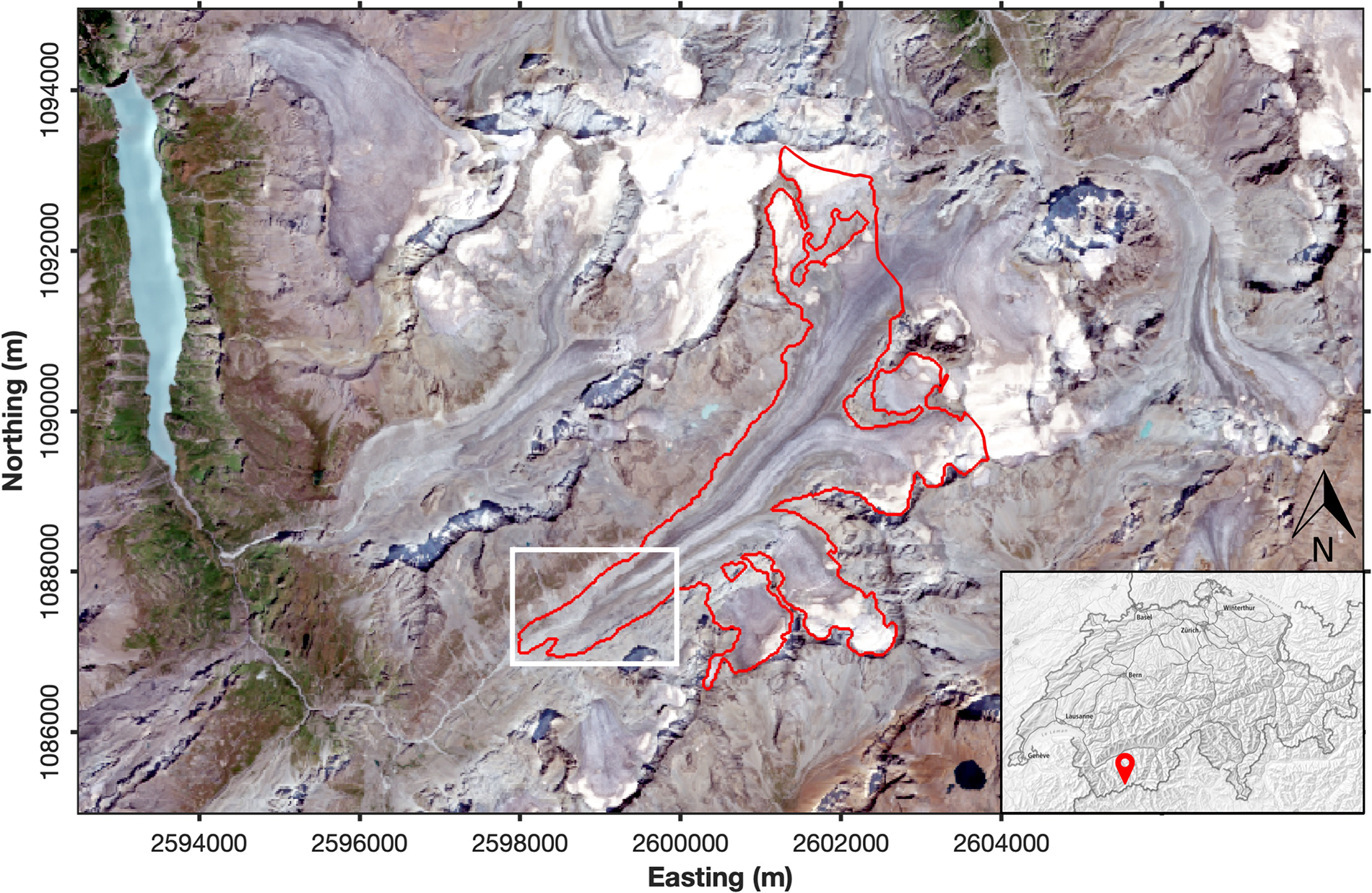
  $6.5\,\mathrm{km}$ (GLAMOS, 1881-2023). It is a temperate valley glacier located in the southern part of the Valais canton, close to the Swiss-Italian border (Fig. 1). The main glacier has its origin at the southern flank of the Pigne d’Arolla and flows southwest into the Haut Val de Bagnes from about $3790\,\mathrm{m}$ to $2500\,\mathrm{m}$ above sea level (a.s.l.), while being fed by several tributary glaciers. Most of the glacier volume is located below the equilibrium line altitude, which divides the glacier into a small accumulation zone and a long flat main tongue. The Otemma Glacier is rapidly retreating as a result of climate warming and has been losing mass faster than most glaciers in the Swiss Alps (Fischer and others, Reference Fischer, Huss and Hoelzle2015). It has been the subject of earlier studies using GPR (Egli and others, Reference Egli, Irving and Lane2021) and radio-tagged particle tracking (Jenkin and others, Reference Jenkin2023) with the aim of mapping the main subglacial channel. Our survey site is located within the lower ablation area between $2500\,\mathrm{m}$ and $2600\,\mathrm{m}$ a.s.l., where the maximum ice thickness in 2022 was around $90\,\mathrm{m}$. Downstream of the survey area, one main subglacial channel emerges at the glacier snout and supplies meltwater to a large turbulent stream known as the Dranse de Bagnes.
Location of the Otemma Glacier (red outline) in Switzerland (red pin on the insert map). The white rectangle shows the area of our study. The glacier outline on the satellite image corresponds to the most recent GLIMS data (GLIMS Consortium, 2005), and is based on satellite imagery from 2015. The background satellite image was obtained from Copernicus Sentinel data (2022). The insert map was obtained from the Swiss Federal Office of Topography (http://map.geo.admin.ch). All coordinates are given in meters in the local Swiss coordinate system (CH1903+ / LV95).

Data acquisition and processing
In the summer of 2022, we acquired 3D GPR, photogrammetry and dye tracing data in the lower ablation area of the Otemma Glacier to study its hydrological system. Each of these measurements and its associated data processing is described in detail below. Information is also provided on hydraulic potential modeling, which was carried out based on larger-scale bed topography measurements derived from helicopter-borne GPR surveys (Grab and others, Reference Grab2021).
3D GPR
GPR acquisition
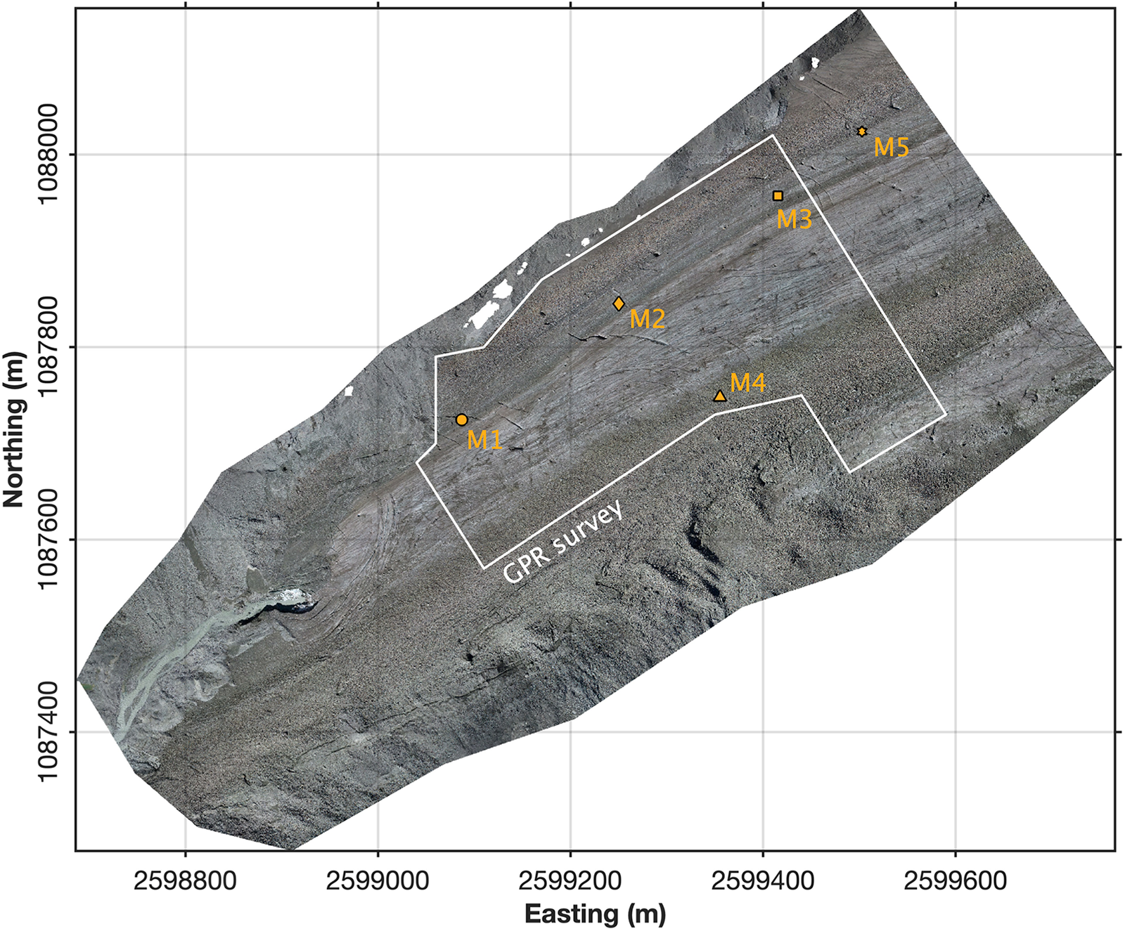
To investigate the englacial and subglacial drainage network, zero-offset, high-density, 3D GPR data covering an area of approximately  $115 000\,\mathrm{m}^{2}$ were acquired near the glacier terminus. The extent of the GPR survey area is shown in Fig. 2. The GPR data were collected over four days (August 2–4 and 6, 2022) using a recently developed UAV-based acquisition system designed for safe and efficient surveying of alpine glaciers (Ruols and others, Reference Ruols, Baron and Irving2023). The survey grid comprises 488 profile lines spaced at $1\,\mathrm{m}$ intervals. This dense line spacing reduces the across-line spatial aliasing of reflected and diffracted arrivals at the antenna’s $80\,\mathrm{MHz}$ center frequency, which corresponds to a dominant wavelength in ice of approximately $2.1\,\mathrm{m}$. The individual GPR profiles are oriented northwest-southeast, perpendicular to the ice flow direction and vary in length between $115\,\mathrm{m}$ and $350\,\mathrm{m}$. In total, more than $115\,\mathrm{km}$ of GPR data were acquired.
Study site close to the glacier terminus. The white polygon indicates the area covered by the GPR survey. The orange symbols mark the locations of moulins that were used for dye tracing experiments. The background orthomosaic was obtained from photogrammetry surveys conducted in September 2022.

During data acquisition, the UAV-based GPR system was flown at a height of approximately  $5\,\mathrm{m}$ above the glacier surface and at a speed of $4\,\mathrm{ms}^{-1}$ using the True Terrain Following navigation system from SPH Engineering (Latvia), which uses real-time radar-altimeter measurements to adjust the flight path so that it closely follows the underlying topography (Ruols and others, Reference Ruols, Baron and Irving2023). With a trace acquisition rate of approximately $14\,\mathrm{Hz}$, stacking each measurement over 5000 times, this configuration yielded more than three GPR traces per meter (Ruols and others, Reference Ruols, Baron and Irving2023). Data were recorded with a temporal sampling interval of $3.125\,\mathrm{ns}$ over a total recording time of $2800\,\mathrm{ns}$, corresponding to a theoretical depth of penetration of approximately $220\,\mathrm{m}$ in glacier ice. Ice thickness in the survey area ranged from approximately $20\,\mathrm{m}$ to $90\,\mathrm{m}$, and allowed for consistent identification of the glacier bed. The GPR profiles were flown with the single, transmit-receive, resistively loaded dipole antenna oriented perpendicular to the flight direction, which has been shown in previous studies to provide stronger and more coherent bed reflections (Langhammer and others, Reference Langhammer, Rabenstein, Bauder and Maurer2017). The UAV, a DJI M300 RTK drone manufactured by Shenzhen DJI Sciences and Technologies (China), is equipped with a real-time kinematic (RTK) global navigation satellite system (GNSS), providing positioning with a horizontal accuracy of approximately $1\,\mathrm{cm}$ and a vertical accuracy of around $2\,\mathrm{cm}$.
GPR processing
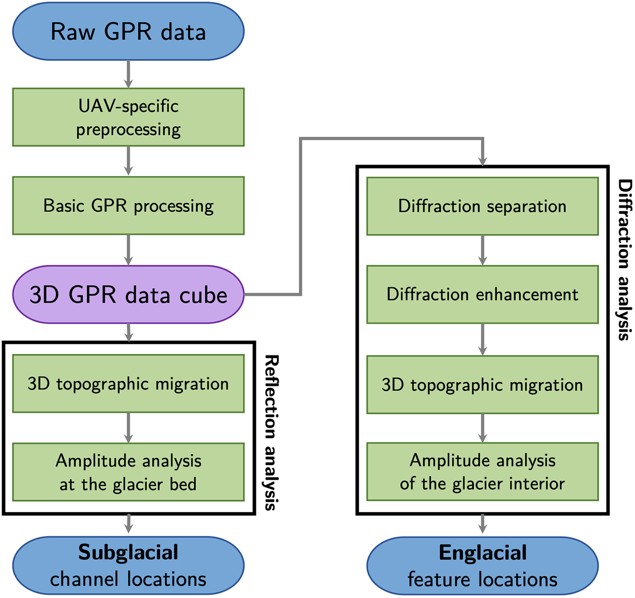
The raw GPR measurements, which are recorded in time, were processed to produce two separate depth-migrated 3D data volumes: a reflection volume to map the topography of the glacier bed and the locations of subglacial channels, and a diffraction volume to identify englacial features. The processing workflow is accordingly divided into two parallel streams to produce these volumes. Both processing streams share an initial set of basic preprocessing steps (Fig. 3).
Overview of the GPR data processing workflow. Left: Reflection analysis stream used to map subglacial channels. Right: Diffraction analysis stream used to identify englacial features. Both streams share a common set of initial preprocessing steps.

Preprocessing
GPR acquisition with our UAV-based system requires additional preprocessing steps beyond those used in conventional surface-based surveys (Ruols and others, Reference Ruols, Baron and Irving2023). In the field, GPR traces and drone navigational data are recorded separately, each tagged with GPS time. The first step is to synchronize these datasets based on the shared timestamps for each flight, such that each recorded GPR trace is associated with full navigational information. Next, the GPR data are segmented into individual profile lines, and binning is performed using the trace positioning data to distribute the GPR measurements evenly along each line. In this regard, we adopted an along-line bin spacing of  $0.4\,\mathrm{m}$ which, given our UAV speed and the GPR sampling rate, ensured a sufficiently high trace density to populate every bin. Stacking the binned profiles side by side produces an initial 3D GPR volume, which requires further positional corrections to address artifacts introduced during UAV acquisition. Discontinuities in the data between profile lines, related to small changes in flight altitude, are corrected using Fourier static adjustments in order to simulate a smooth acquisition surface. Lateral positioning corrections are applied to address systematic shifts between odd- and even-numbered profiles related to small internal timing delays specific to our GPR controller. The latter is accomplished using a constrained cross-correlation algorithm that maximizes continuity between adjacent profiles (Ruols and others, Reference Ruols, Baron and Irving2023). For full details on these preprocessing steps, see Ruols and others (Reference Ruols, Baron and Irving2023, Reference Ruols, Klahold, Farinotti and Irving2025).
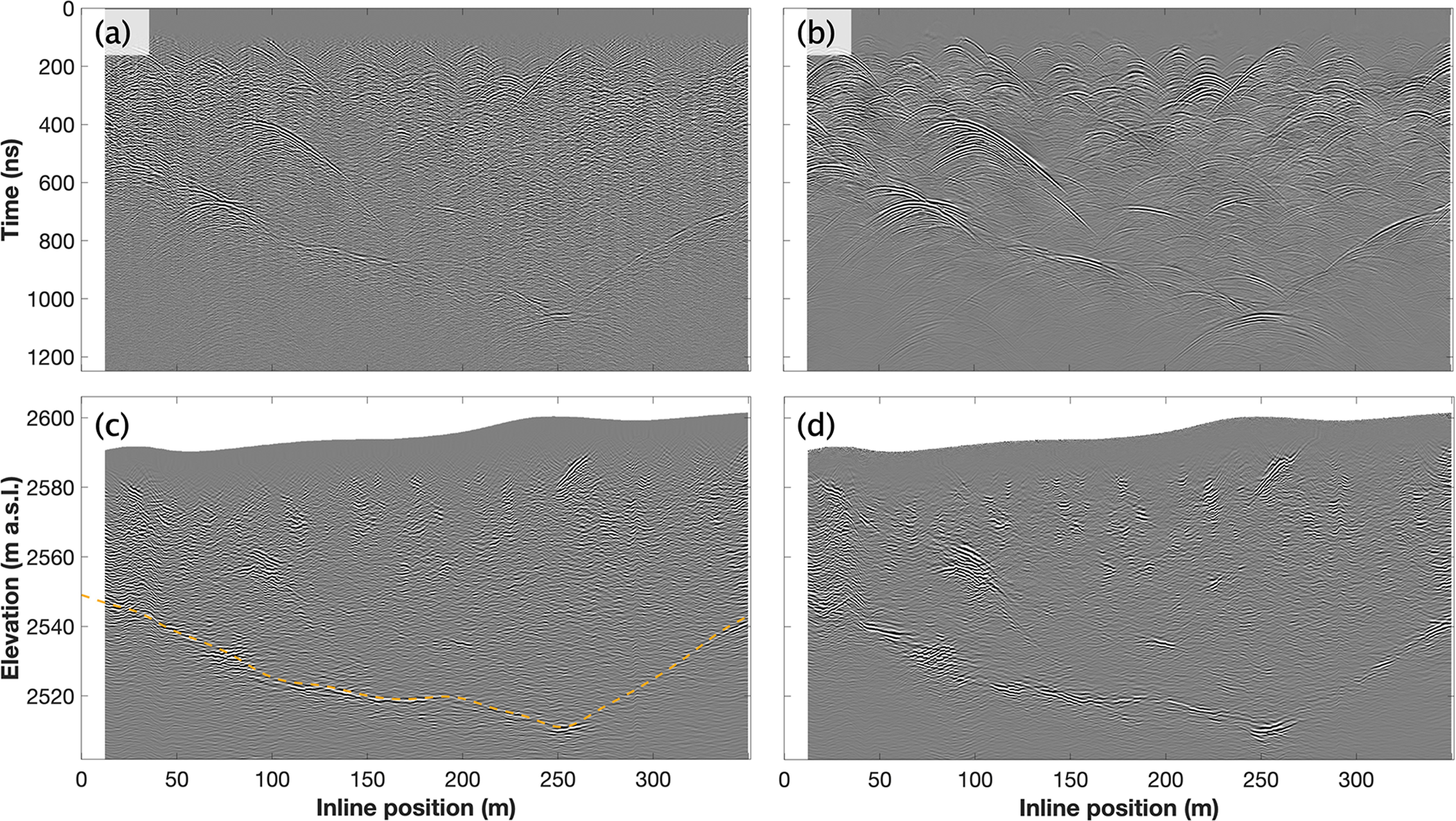
After the drone-specific processing described above, the following standard GPR processing is applied to each profile: (i) mean trace removal using a 100-trace sliding window, (ii) de-wow using a 35-point residual median filter, (iii) 4 times temporal densification via Fourier transform interpolation, (iv) time-zero correction, (v) application of a smooth mute to the initial part of each trace and (vi) a second mean trace removal using a 15-trace sliding window applied to the upper portion of the profiles to further suppress residual ringing artifacts. Figure 4a shows an example GPR survey line after application of these steps, where we observe a clear reflection from the glacier bed as well as numerous diffraction hyperbolas arising from englacial scatterers.
Demonstration of the GPR processing for one example inline profile located at a crossline position of  $459\,\mathrm{m}$: (a) after preprocessing; (b) result from (a) after diffraction separation and enhancement; (c) result from (a) after 3D topographic migration, time-to-depth conversion and topographic correction, with the orange line indicating the smooth bedrock surface model developed from the picked glacier bed reflection; (d) result from (b) after 3D topographic migration, time-to-depth conversion and topographic correction.

Reflection analysis
To image the subglacial drainage system, we first follow Egli and others (Reference Egli, Irving and Lane2021) and Ruols and others (Reference Ruols, Klahold, Farinotti and Irving2025) and apply 3D topographic time migration to the GPR data using the algorithm developed by Allroggen and others (Reference Allroggen, Tronicke, Delock and Böniger2015), which is based on the general Kirchhoff scheme presented in Schneider (Reference Schneider1978). To account for the distance between the GPR antenna and the glacier surface, we consider a two-layer migration velocity model. The upper layer represents air, with a velocity of  $0.3\,\mathrm{m\,ns}^{-1}$, whose thickness is determined from the UAV’s altimeter data following Ruols and others (Reference Ruols, Klahold, Farinotti and Irving2025). The lower layer corresponds to glacier ice, for which we assume a constant velocity of $0.16\,\mathrm{m\,ns}^{-1}$, as is commonly done in glaciological GPR studies (e.g., Bradford and others, Reference Bradford, Nichols, Mikesell and Harper2009; Langhammer and others, Reference Langhammer, Rabenstein, Bauder and Maurer2017; Church and others, Reference Church, Grab, Schmelzbach, Bauder and Maurer2020). Velocity testing showed that this value provides the most coherent collapse of diffraction hyperbolas during migration. Additional testing indicated that a migration aperture of $40\,\mathrm{m}$ effectively collapses diffraction hyperbolas in the dataset. Following migration, the same two-layer velocity model is used to convert the data from time to depth, and the position of each trace is shifted vertically to account for the topography of the acquisition surface. Figure 4c shows the example profile from Fig. 4a after migration, time-to-depth conversion and topographic correction.
To map subglacial channels, we use the migrated 3D GPR volume to delineate and analyze the glacier bed reflection (Church and others, Reference Church, Bauder, Grab and Maurer2021; Egli and others, Reference Egli, Irving and Lane2021; Ruols and others, Reference Ruols, Klahold, Farinotti and Irving2025). Channels filled with water or air produce a stronger contrast in dielectric permittivity with the glacier ice than the surrounding bedrock, which results in a greater radar reflection coefficient in the channel locations. To this end, we manually pick the ice–bed interface on the individual migrated GPR profiles, and we use local linear regression to produce a smooth bedrock surface model (Fig. 4c). To quantify reflection strength at the bed, we calculate the instantaneous amplitude of each trace using the Hilbert transform (Taner and others, Reference Taner, Koehler and Sheriff1979; Chopra and Marfurt, Reference Chopra and Marfurt2007), and identify its maximum over a vertical  $2\,\mathrm{m}$ window centered on the identified bedrock location (Egli and others, Reference Egli, Irving and Lane2021; Ruols and others, Reference Ruols, Klahold, Farinotti and Irving2025). The resulting maximum instantaneous amplitude values typically exhibit a small but systematic decrease with increasing ice thickness, reflecting the greater loss of radar energy with increasing propagation distance. To correct for this effect, we apply robust linear regression to estimate and remove the thickness-related trend. We acknowledge that some redistribution of energy by englacial reflections is possible and may locally influence the amount of energy reaching the bed; however, in practice, we have not found this to limit the identification of subglacial channels in our data. We further acknowledge that the data were collected over several days, but we do not observe diurnal variations in the nature of the data that would affect the imaging or interpretation of the larger-scale drainage network. The final product is a 2D map of maximum reflection strength along the glacier bed.
Diffraction analysis
GPR data acquired over temperate glaciers are typically rich in diffraction events caused by englacial heterogeneities that act as either point or line scatterers of the radar energy (Murray and others, Reference Murray, Stuart, Fry, Gamble and Crabtree2000; Schaap and others, Reference Schaap, Roach, Peters, Cook, Kulessa and Schoof2020; Ogier and others, Reference Ogier2023). Imaging these events in 3D and analyzing their spatial distribution can serve as a potentially powerful tool to characterize the glacier’s drainage system, as englacial channels and voids will act as strong scatterers due to the marked contrast in dielectric permittivity with their surroundings. To identify englacial features, we thus focus on diffracted energy within the preprocessed 3D GPR data cube. To distinguish diffraction signals from reflections and noise in a fully data-driven manner, we adopt the coherent stacking scheme of Schwarz and Gajewski (Reference Schwarz and Gajewski2017) and Schwarz (Reference Schwarz2019). The corresponding workflow comprises two main steps: diffraction separation and diffraction enhancement. For computational efficiency, both steps are applied to individual 2D GPR profiles. The processed profiles are then reassembled into a 3D data cube, which is subsequently migrated in 3D to accurately image diffracting features.
In the first step, we separate diffracted energy from reflected signals by performing a coherent summation within a defined aperture around each data sample. Local slopes and curvatures of emerging wavefronts are estimated directly from the data using a coherence maximization procedure. Since reflections generally exhibit lower slope and curvature values than diffractions, we can distinguish between the two using threshold-based filtering. We apply directional stacking, which inherently favors the dominant reflected arrivals, and combine this with a slope-based filter to estimate the reflected component. The estimated reflected wavefield is then subtracted from the original data, resulting in a GPR profile that contains primarily diffracted energy, along with residual noise (Schwarz and Gajewski, Reference Schwarz and Gajewski2017; Schwarz, Reference Schwarz2019). In the second step, to further enhance the diffraction signal, we re-estimate slope and curvature attributes from the resulting diffracted wavefield and use them to guide a second coherent stacking step, this time optimized to emphasize locally coherent diffraction events. Figure 4b shows the preprocessed example profile from Fig. 4a after diffraction separation and enhancement, where we see that the diffractions can be much more easily identified and that clutter-type noise in the section has been greatly reduced.
The separated and enhanced diffraction data are subsequently imaged through 3D topographic migration using the same algorithm as in the reflection analysis (Allroggen and others, Reference Allroggen, Tronicke, Delock and Böniger2015). For this step, we employ a slightly larger migration aperture of  $50\,\mathrm{m}$ to better capture the wider spread of diffracted energy in the enhanced data, while all other migration parameters remain unchanged. Figure 4d presents the diffraction enhanced survey profile from Fig. 4b after migration, time-to-depth conversion and topographic correction, where we observe that the migration algorithm effectively collapses diffraction hyperbolas around their primary scattering points.
The separated, enhanced and migrated GPR diffraction volume is analyzed to identify drainage pathways within the glacier interior, which typically correspond to regions of high amplitude that exhibit strong spatial continuity across multiple survey profiles. To this end, similar to the subglacial analysis, we first calculate the instantaneous amplitude of each trace in the volume using the Hilbert transform, which serves as a proxy for scattering strength. Next, we apply a thresholding step by selecting the 99th percentile of normalized amplitude values, in order to isolate only the highest-amplitude features likely to represent strong scatterers such as channels. We then use a 3D elliptical structuring element on the resulting binary volume to perform morphological closing, connecting nearby high-amplitude regions. Connected components are extracted from the closed volume using 26-connectivity. Finally, for each component, we compute geometric properties such as volume and principal axis length, and retain only elongated structures having a principal axis length greater than 30 voxels and a volume exceeding 2500 voxels, yielding a binary mask of candidate englacial channels with unique feature IDs.
Photogrammetry
High-resolution UAV-based photogrammetry surveys were conducted on September 12, 2022, to generate an orthomosaic and a digital elevation model (DEM), providing surface information to support the interpretation of the UAV-based GPR data. A DJI Phantom 4 Pro UAV was flown at altitudes between 65 and 80 meters above the take-off point, capturing nadir and oblique imagery. Approximately 2,000 images were acquired. A differential GPS (Topcon GR-5) was used to survey the precise positions of 15 ground control points (GCPs), along with 22 additional check points (CPs) used for model validation.
The data were processed using the Agisoft Metashape Professional Edition 2.1.2 software, largely following the guidelines provided in the user manual. The photogrammetric processing workflow included image quality assessment, photo alignment, point cloud generation and model optimization based on GCPs. Photo alignment was performed using a key point limit of 120,000 and a tie point limit of 12,000, with adaptive camera model fitting enabled. Dense point clouds were generated using depth maps at high quality with moderate depth filtering. The dataset was georeferenced using the Swiss coordinate system (CH1903+ / LV95). The final DEM has a spatial resolution of 4.96 cm/pixel, whereas the resolution of the orthomosaic is 2.48 cm/pixel.
Dye tracing
To investigate englacial and subglacial drainage connections in our study region, we conducted six dye tracing experiments using two fluorescent tracers: rhodamine WT and fluorescein. The experiments were conducted between August 2 and 6, with individual injections performed at different times of day. The tracers were injected simultaneously into selected pairs of moulins in the survey area (M1–M5; Fig. 2), which allows us to compare the connectivity of the moulins to the subglacial system and the efficiency of the drainage pathways. The moulins were selected because of their high observed meltwater input. Injection times were synchronized to the second to ensure similar flow and discharge conditions, which vary substantially throughout the day, even on the time scale of minutes. Repeat experiments were conducted for the moulin pair M1–M2 to assess the consistency of the results across multiple days and times of day. For all experiments, the dye concentrations were measured in the main outlet stream close to the glacier terminus with a fluorometer (Albillia GGUN-FL30) recording at  $6\,\mathrm{s}$ intervals after dye injection. Breakthrough curves were generated by applying a $60\,\mathrm{s}$ running average filter to the measured dye concentrations, subtracting any instrument bias to read a background value of zero, and scaling by the maximum dye concentration value over all breakthrough curves of the same dye type. The curves were analyzed following Nienow and others (Reference Nienow, Sharp and Willis1996a) in order to estimate the arrival time ( $t_a$), the peak arrival time ( $t_m$), and the water throughflow velocity ( $u$).
$u$).
Hydraulic potential modeling
As an independent method to assess the plausibility of the subglacial drainage system inferred from the 3D GPR data, we estimated the likely subglacial water routing following the approach of Shreve (Reference Shreve1972), which assumes that subglacial flow paths are governed by the spatial distribution of the hydraulic potential at the bed,  $\phi$, given by
 \begin{equation}
\phi = \rho_w g z_b + p_w, \quad \text{with} \quad p_w = \alpha \rho_i g (z_s - z_b),
\end{equation}
\begin{equation}
\phi = \rho_w g z_b + p_w, \quad \text{with} \quad p_w = \alpha \rho_i g (z_s - z_b),
\end{equation}where  $p_w$ is the subglacial water pressure at the ice-bed interface, assumed to be a fraction $\alpha$ of the ice overburden pressure, $\rho_w$ is the density of water ( $1000\,\mathrm{kg\,m}^{-3}$), $\rho_i$ is the density of ice ( $917\,\mathrm{kg\,m}^{-3}$), $g$ is gravitational acceleration ( $9.81\,\mathrm{m\,s}^{-2}$), $z_s$ is the ice surface elevation and $z_b$ is the bedrock elevation. Here, we assumed $\alpha = 1$, which corresponds to the common assumption that water pressure is equal to ice overburden pressure (i.e., a steady-state or ‘full’ subglacial water system). We used surface and bedrock topography data from Grab and others (Reference Grab2021) at $10\,\mathrm{m}$ horizontal resolution for this analysis, rather than our own derived surface and bed topography data over the GPR survey region, because coverage across the entire glacier domain was required to calculate flow pathways beyond the limited survey area.
From the calculated hydraulic potential field, we derived local hydraulic gradients and flow directions using the TopoToolbox package in MATLAB (Schwanghart and Kuhn, Reference Schwanghart and Kuhn2010; Schwanghart and Scherler, Reference Schwanghart and Scherler2014). Treating the hydraulic potential as an analog to topographic elevation, the D8 (Deterministic Eight-Neighbor) flow routing algorithm (O’Callaghan and Mark, Reference O’Callaghan and Mark1984) was employed, which routes the flow from each grid cell to its single steepest downslope neighbor. Once the flow directions were determined, we applied the flowaccumulation function to estimate the upstream contributing area for each grid cell, which yields insight into likely subglacial drainage networks and relative discharge magnitudes.
Results
Subglacial drainage system
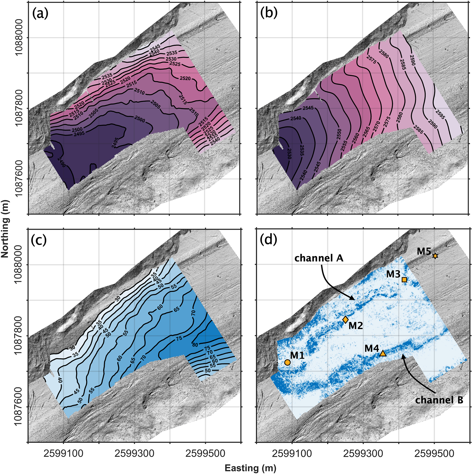
Figure 5 presents the results of our GPR reflection analysis. In Fig. 5a, we show the glacier bed elevation determined from manual picking of the ice-bed interface along each profile in the migrated 3D reflection volume. The glacier surface elevation is shown in Fig. 5b. Taking the difference between these quantities yields the ice thickness in the survey region (Fig. 5c), which is seen to vary between  $20\,\mathrm{m}$ and $90\,\mathrm{m}$. In Figure 5d, we show the 2D map of normalized reflection strength along the glacier bed. Here, we can identify two distinct zones exhibiting higher amplitude reflections than their surroundings, interpreted as potential subglacial channels, that run from northeast to southwest across the entire GPR survey region, broadly aligned with the direction of glacier flow. The northern zone, hereafter referred to as channel A, initially appears weakly up-glacier in the vicinity of moulin M3. As it continues down-glacier, its signature becomes stronger and, after meandering slightly, it follows a trajectory roughly parallel to the northern glacier flank. Near the western edge of our survey region, channel A exhibits a pronounced southward meander around the location of moulin M1. The second distinct, high-reflectivity zone to the south, hereafter referred to as channel B, is clearly visible in the eastern-most part of the survey region. It initially follows the deepest section of the basal topography, undergoes a sharp bend, and then continues along a straight trajectory that passes below moulin M4. Further downstream, channel B appears to widen and eventually meanders northward to coalesce with channel A near the western edge of the survey area, where an ice-marginal channel is visible further along the inferred trajectory (Fig. 2). Notably, our dye tracing moulins also appear to be positioned broadly above these channels, reinforcing the link between the GPR-identified basal features and glacier drainage. Additionally, along the north and south boundaries of the survey region, we observe further high-amplitude zones. However, the available data do not allow us to determine whether these features are representative of actual basal conditions or artifacts introduced during migration.
GPR reflection analysis results: (a) glacier bed elevation (m a.s.l.); (b) glacier surface elevation (m a.s.l.); (c) calculated ice thickness (m); (d) normalized reflection strength along the glacier bed (blue = stronger). All images are superposed on a hillshade of the DEM from September 2022.

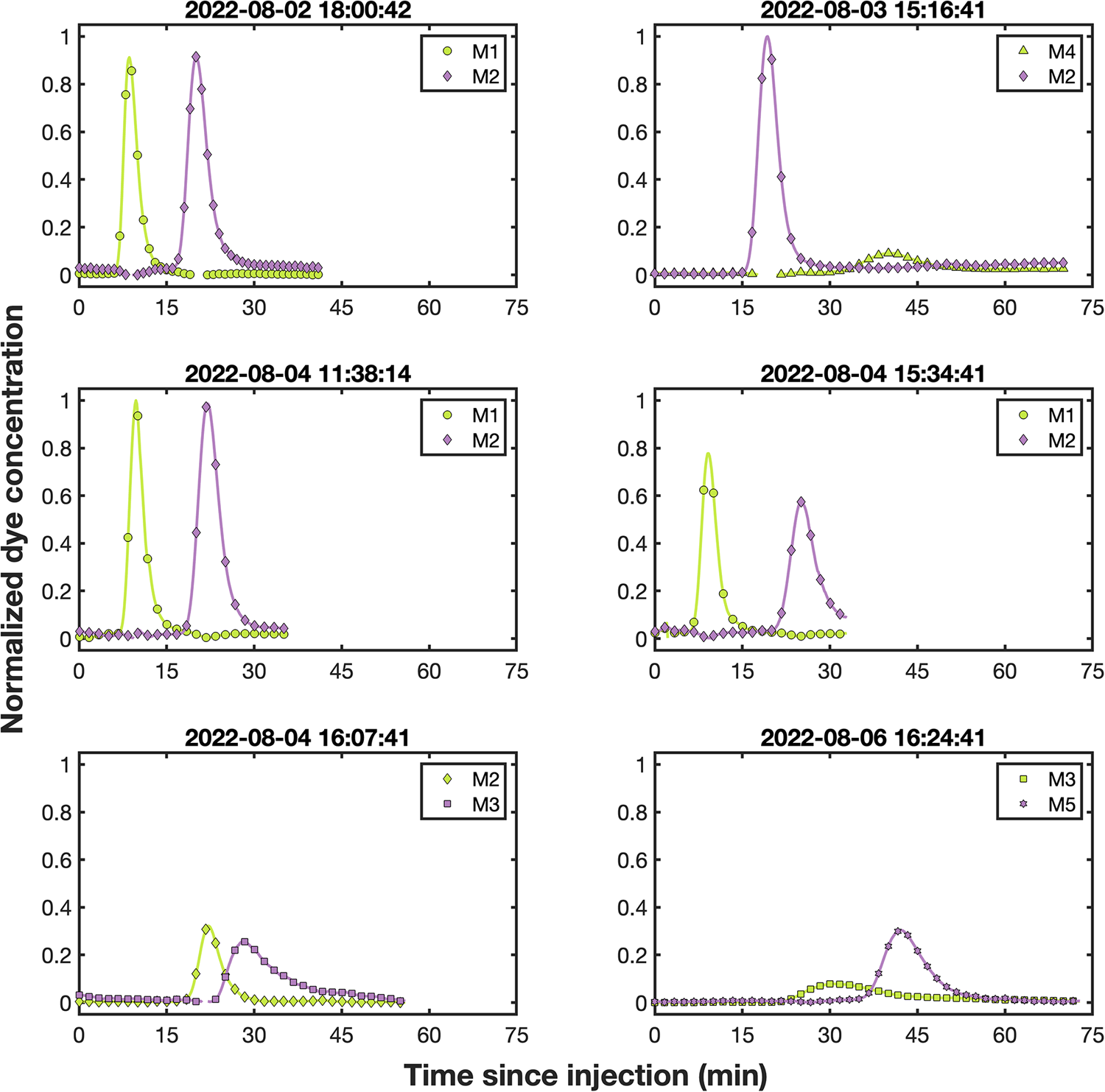
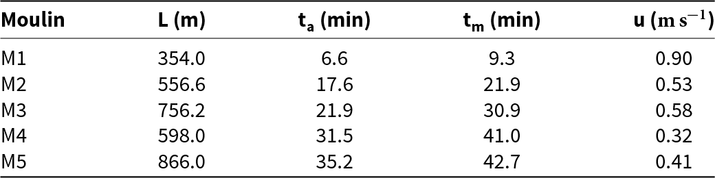
Figure 6 shows the breakthrough curves obtained for the six dye tracing experiments that were conducted for various pairs of moulins. Table 1 presents metrics obtained from a quantitative analysis of these curves. We observe a clear dye breakthrough for all injected moulins (M1–M5), indicating that each is hydraulically connected to the main subglacial drainage system. This is also reflected in the rapid throughflow velocities ( $u \gt 0.2\,\mathrm{m\,s}^{-1}$, Burkimsher (Reference Burkimsher1983)) for all injection points, namely, for moulins M1, M2, M3 and M5, which are likely connected to channel A, and for moulin M4, which is presumably linked to channel B. Overall, dye arrival times increase progressively with distance up-glacier, reflecting longer travel paths for upstream moulins. One notable exception is moulin M4, which exhibits a markedly greater arrival time and a lower throughflow velocity than moulin M2, despite being located at a comparable distance from the glacier snout. This suggests that either moulin M4 has a less direct connection to the subglacial channel, or that channel B is less hydraulically efficient than channel A. Channel B may indeed exhibit a greater potential for dispersion than channel A, as suggested by the broader breakthrough curve of moulin M4 compared with moulin M2.
Dye concentration over time for six dye tracing experiments involving pairs of moulins. Colors and symbols are representative of the injected dye (lilac: rhodamine WT, green: fluorescein) and moulin, respectively.

Dye tracing metrics calculated from the breakthrough curves presented in Figure 6 following Nienow and others (Reference Nienow, Sharp and Willis1996a). Shown are the straight-line distance between the moulin and the glacier outlet ( $L$), the tracer arrival time ( $t_a$), the peak arrival time ( $t_m$) and the water throughflow velocity ( $u$). For moulins with repeat injections, mean values of the metrics were calculated.

Another experiment that merits closer attention is the comparison between the breakthrough curves of moulins M3 and M5. A sharp, well-defined breakthrough curve is observed for moulin M5, whereas moulin M3 exhibits a broader curve with a longer tail (Fig. 6). This contrast suggests that M5 may drain directly into the main subglacial conduit, whereas M3 could be connected via a smaller tributary channel. However, moulin M5 lies outside the GPR survey area, making it difficult to verify its connection to the main drainage system. This inference is further limited by the fact that only a single dye tracing experiment was conducted for the M3–M5 pair, and the resulting travel times may have been affected by local injection conditions. Additionally, while dye tracing provides valuable insights into subglacial drainage efficiency, it is important to recognize that dye must first traverse the englacial system before reaching the bed. This englacial component is often neglected in analyses and may introduce uncertainty into interpretations based solely on travel time and flow velocities.
Finally, repeat tracer injections for moulin pair M1–M2 reveal consistent breakthrough behavior across different times of day and on separate days (evening on August 2, midday and afternoon on August 4). While slight variations in curve shape and timing are observed, moulin M1 consistently exhibits an earlier arrival than moulin M2, and both moulins produce two sharp breakthrough peaks. This suggests a temporally stable drainage configuration during the observation period, demonstrating the robustness of dye tracing across the days of data collection and justifying its use for inferring overall drainage characteristics.
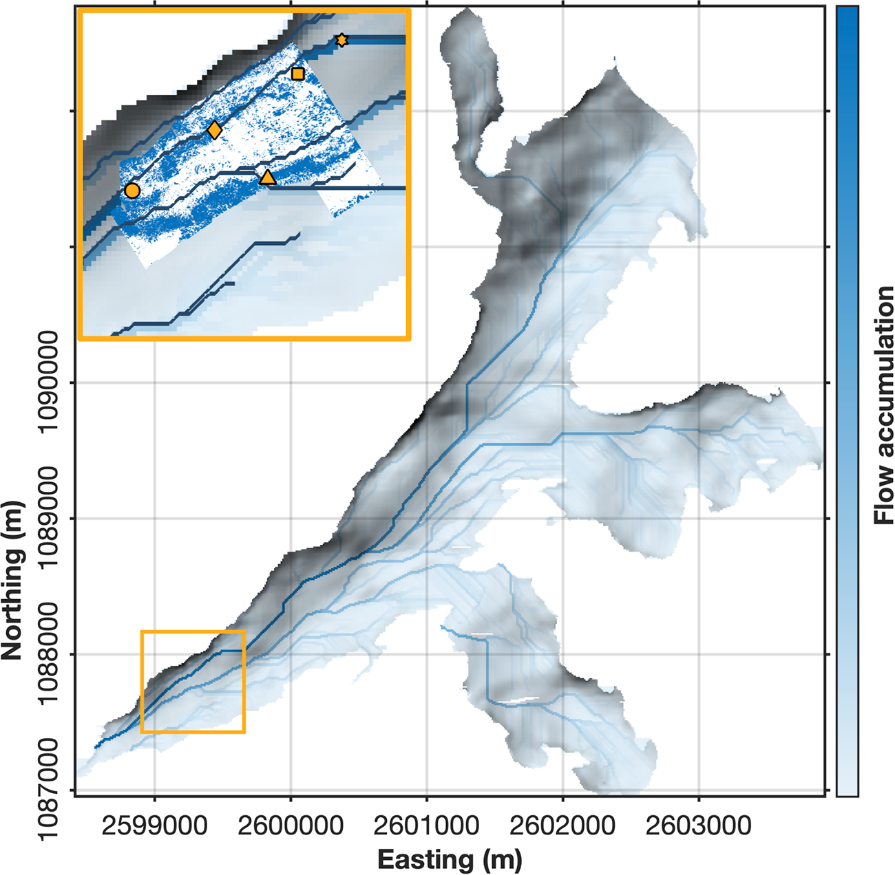
Figure 7 presents the results of our hydraulic potential modeling, and highlights the most probable locations of subglacial channels based on the underlying bedrock topography and ice thickness data of Grab and others (Reference Grab2021). Two main channels can be identified, which merge downstream; the northern channel appears to accumulate a greater volume of water and may function as the primary drainage pathway. We observe that the modeled subglacial drainage network exhibits strong spatial correspondence with the regions of increased GPR bed reflection amplitude (Fig. 7; inset), suggesting that the drainage patterns inferred from the GPR data are physically plausible and likely represent actual subglacial flow paths. Again, dye tracing moulins M1–M5 lie broadly atop the modeled subglacial channels. However, it is important to note that this analysis reflects a stationary and steady-state assumption, where the hydraulic potential field is considered time-invariant, which is a strong simplification. In reality, subglacial water pressure and routing pathways vary temporally due to meltwater input fluctuations, ice dynamics and evolving drainage system configurations. Therefore, the modeled pathways represent only a static and idealized scenario.
Most probable subglacial channel locations according to the Shreve hydraulic potential model. Shading reflects the amount of flow accumulation, with darker blue representing higher accumulated flow and thus a higher likelihood of subglacial drainage pathways. The inset shows a zoom of the GPR survey area with an overlay of the normalized GPR reflection strength at the glacier bed. Orange symbols indicate the locations of dye tracing moulins, whereas dark blue lines mark the main flow accumulation drainage paths.

Englacial drainage system
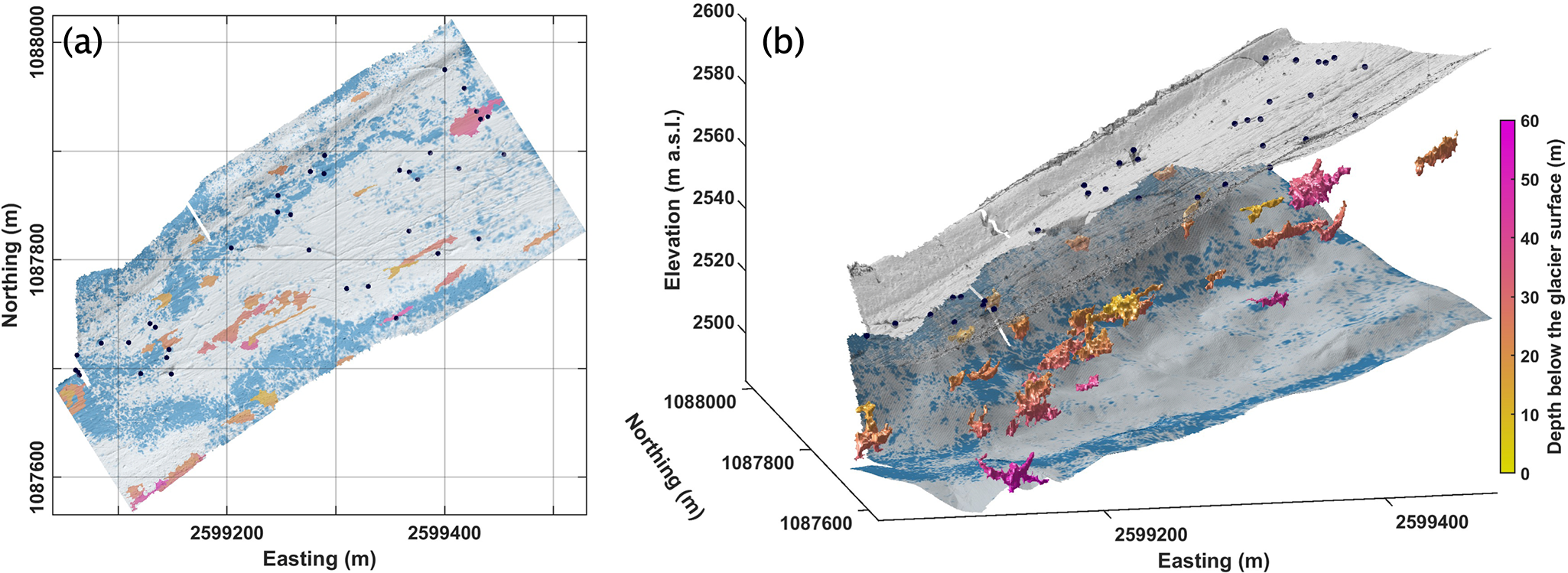
Figure 8 presents the results of our diffraction analysis, which yields a 3D map of connected zones of high scattering amplitude that we interpret as components of the englacial drainage network. From a top-down perspective, many of the englacial features exhibit a linear alignment roughly along the glacier flow direction (Fig. 8a). In the 3D view, we see that the internal architecture is complex, consisting of a number of variable-sized features that likely share further connections that are not imaged (Fig. 8b). Note that many of the identified englacial features and moulin locations do not directly overlie the main subglacial channels identified in our bed reflection analysis. This, along with the observation that the englacial channels span large horizontal distances, suggests that meltwater is not routed vertically from the surface to the bed, but instead travels laterally through the englacial system, often over considerable distances, before entering the main subglacial channels.
3D map of spatially connected high-amplitude zones in the GPR diffraction instantaneous amplitude volume. The glacier surface is provided by the DEM from September 2022. The glacier bed is provided by our GPR bed reflection analysis, and is shaded with the map of normalized reflection strength. Black dots at the glacier surface indicate moulin locations identified on the orthomosaic (Fig. 2). (a) Top view; (b) side view.

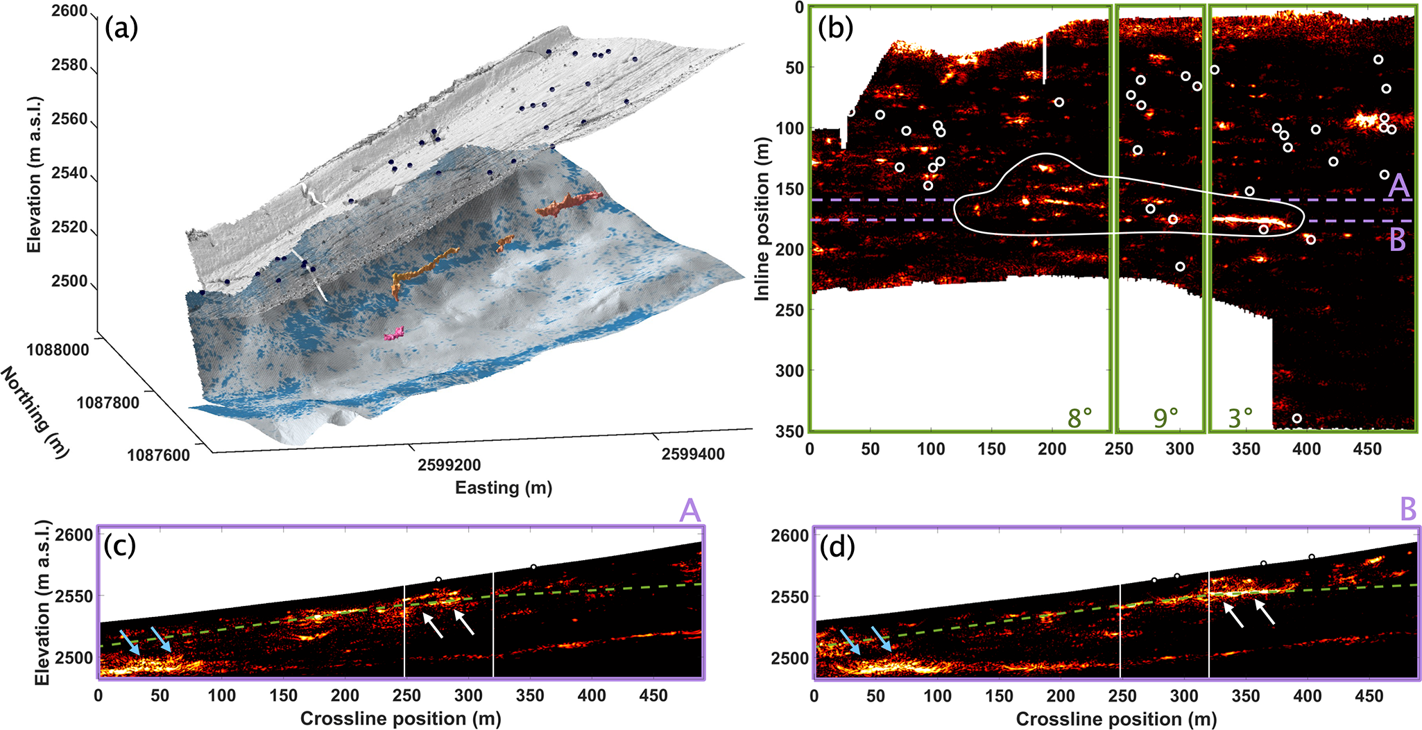
To explore further, we highlight two representative features, isolated using their feature IDs, which are presented in Figs. 9 and 10. The first feature (Fig. 9) is a well-defined englacial channel oriented approximately along the glacier flow direction (i.e., parallel to the crossline axis), with a total length of nearly  $200\,\mathrm{m}$. Located about $20\,\mathrm{m}$ below the ice surface, the channel maintains a consistent, linear geometry but exhibits notable variations in its longitudinal slope that likely influence internal water flow dynamics. In its uppermost section, the channel descends gently with a slope of approximately $3^{\circ}$ over a distance of approximately $80\,\mathrm{m}$. The gradient then steepens significantly to around $9^{\circ}$ over $70\,\mathrm{m}$, before decreasing slightly to about $8^{\circ}$ over $50\,\mathrm{m}$. Moulins observed at the surface above the channel suggest that it may be actively fed by these surface meltwater inputs. In its lower section, at a crossline position of $250\,\mathrm{m}$, the englacial channel appears to become more diffuse, connecting with a set of narrower, parallel side channels (not displayed in the reduced 3D view in Fig. 9a). These smaller conduits run roughly in the same direction and may function as secondary flow paths, suggesting a sectional branching structure within the englacial system. Downstream of this, at a crossline position of around $170\,\mathrm{m}$ (Fig. 9c), the main englacial channel exhibits a sudden vertical drop into a localized region of high reflectivity, which we interpret as a potential water pooling area. While we do not directly observe a connection to the subglacial system within the GPR volume, it is likely that this channel ultimately links to the basal drainage network, given its alignment and downward trajectory. This interpretation is supported by the presence of a stronger glacier bed reflection in the crossline radar profiles, especially near the terminus, where high reflectivity is consistent with the position of the subglacial channel identified in previous analyses.
Englacial feature 1: (a) 3D map of the isolated feature; (b) composite plan view of three slices through the diffraction instantaneous amplitude volume at different angles with respect to the horizontal; (c) crossline slice through the volume at an inline position of  $161\,\mathrm{m}$; (d) crossline slice through the volume at an inline position of $176\,\mathrm{m}$. Dots denote identified moulin locations. White arrows and outline highlight the englacial channel. Blue arrows indicate the region of stronger bed reflection amplitude.

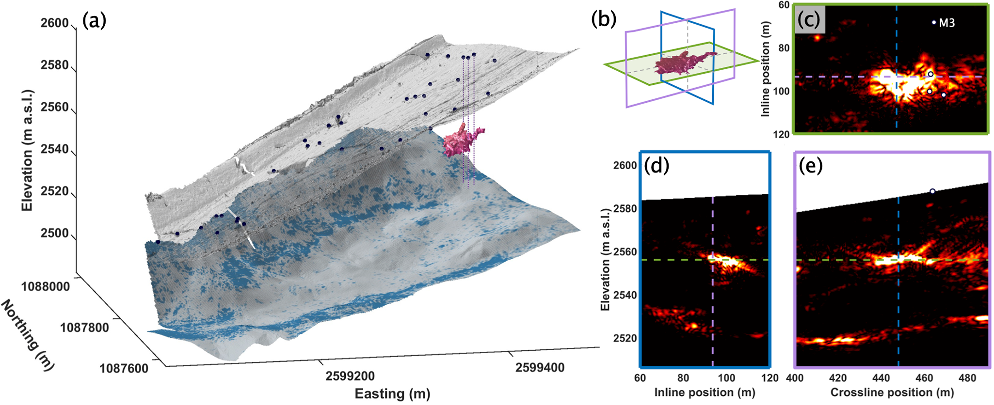
The second feature (Fig. 10) is interpreted as a localized englacial pooling structure about  $30\,\mathrm{m}$ below the glacier surface, approximately $20\,\mathrm{m}$ wide in the cross-glacier direction and $50\,\mathrm{m}$ long along the direction of glacier flow. The feature is clearly resolved in both the inline and crossline depth sections in Figs. 10d and 10e, respectively, as shown by a concentrated zone of high reflectivity within the ice. Several moulins are located directly above and around this feature, suggesting active surface meltwater input. It is likely that water is routed downwards beneath at least one of these moulins into the pooling region. Additionally, the feature appears to be fed by a horizontal englacial connection from further up-glacier, as indicated by the smeared-out high-amplitude zone near the uppermost edge of the survey area. The pooling structure is situated just above the location of the main subglacial channel, making a hydraulic connection between the two likely. However, the identification of vertical conduits is inherently constrained by the limitations of our GPR survey geometry, which restricts sensitivity to near-vertical features. Notably, this pooling feature lies adjacent to moulin M3, one of the dye tracing injection points. Yet, the slight offset of moulin M3 suggests that more likely one of the adjacent moulins and not moulin M3 directly feeds the pooling feature. The connection from moulin M3 may be more complex or less efficient, potentially contributing to the higher dispersion observed in the dye tracing results.
Englacial feature 2: (a) 3D map of the isolated feature; (b) geometry of the presented data slices; (c) horizontal slice through the diffraction instantaneous amplitude volume at an elevation of  $2556\,\mathrm{m}$ a.s.l.; (d) inline slice through the volume at a crossline position of $448\,\mathrm{m}$; (e) crossline slice through the volume at an inline position of $94\,\mathrm{m}$. Dots denote identified moulin locations.

Discussion
This study integrates high-density 3D GPR, dye tracing, photogrammetry and hydrological modeling to investigate the englacial and subglacial drainage system of a temperate alpine glacier. With regard to the subglacial network, all methods consistently support the hypothesis of two main subglacial pathways beneath the study area (channels A and B). The positions of these channels identified from the GPR data correspond well with the flow paths estimated from our hydraulic potential analysis. The dye tracing experiments confirm rapid throughflow for most moulins, supporting the existence of efficient subglacial routing, particularly via channel A. Channel B exhibits higher dispersion and lower velocities, suggesting more distributed or complex drainage characteristics, with potential storage zones or side connections that delay tracer transport compared to the more efficient, well-channelized flow in channel A. With regard to the englacial drainage network, our 3D GPR diffraction analysis reveals a structurally complex system within the ice, characterized by defined channels with variable slopes, localized pooling zones and branching networks. These features indicate that meltwater is not routed directly vertically from the surface to the bed, but rather travels considerable distances englacially before reaching the subglacial system. The spatial configuration of the identified englacial drainage pathways suggests that the englacial structures feed into the imaged subglacial pathways, although the exact points of connection remain unresolved in our GPR data. Despite the use of high-density 3D GPR, spatial resolution remains constrained by the radar wavelength and the inherent limitations of migration in complex glacial environments. As a result, features smaller than 1–2 m may not be fully resolved, contributing to uncertainties in mapping fine-scale drainage connectivity.
A key contribution of our study is the high-resolution, 3D imaging of lateral englacial routing and localized pooling structures within an active, hydrologically connected glacier system. While it is now recognized that meltwater does not always travel vertically from surface moulins directly to the bed (e.g., Gulley and others, Reference Gulley, Benn, Screaton and Martin2009b; Temminghoff and others, Reference Temminghoff, Benn, Gulley and Sevestre2019; Schaap and others, Reference Schaap, Roach, Peters, Cook, Kulessa and Schoof2020), few studies have visualized these pathways in such detail. The prominent englacial channel feature (Fig. 9) exhibits slope variations that may influence flow velocity, possibly accelerating drainage through the steeper sections while encouraging temporary water retention or pooling where gradients shift. In conjunction with the second key feature, the localized pooling structure (Fig. 10), these observations suggest that englacial conduits may function as temporary storage reservoirs or slow-release pathways, potentially modulating the timing and variability of meltwater reaching the bed. This has important implications for interpreting dye tracing data, which typically assume direct surface-to-bed flow and may underestimate englacial transport delays.
The GPR-based methodology presented in this work may also contribute to the refinement of glacier hydrology models in the future by providing empirical constraints on the spatial organization of internal water pathways. By imaging englacial structures that likely govern subglacial water delivery, we provide observational support for theoretical models that incorporate englacial routing and storage (e.g., Bartholomaus and others, Reference Bartholomaus, Anderson and Anderson2008; Reference Bartholomaus, Anderson and Anderson2011; Hewitt, Reference Hewitt2013; Werder and others, Reference Werder, Hewitt, Schoof and Flowers2013), and offer evidence to improve their representation in large-scale simulations. The observed spatial offset between some moulin locations and subglacial channel positions indicates that surface inputs alone are not reliable predictors of basal water entry points. Consequently, our results challenge the simplifications made in many subglacial hydrology models that treat moulin input as a point source at the ice-bed interface (e.g., Werder and others, Reference Werder, Hewitt, Schoof and Flowers2013; de Fleurian and others, Reference de Fleurian2018; Sommers and others, Reference Sommers, Rajaram and Morlighem2018), and underscore the need for models to include englacial transport processes, potentially using constraints on typical englacial pathway lengths such as those revealed by our observations. Given that englacial storage can exert an important control on pressure dynamics within the subglacial drainage system (Flowers and Clarke, Reference Flowers and Clarke2002a), accounting for these processes is crucial for accurate simulations of meltwater-driven glacier behavior.
Our study further demonstrates the value of high-density 3D GPR surveys for mapping both englacial and subglacial drainage structures. The ability to visualize and analyze the internal hydrological architecture in three dimensions provides critical insights that are not accessible through traditional 2D transects or indirect methods alone. Despite their clear potential, such 3D datasets remain rare in glaciological research, primarily because data acquisition has been time-consuming and logistically challenging (e.g., Church and others, Reference Church, Grab, Schmelzbach, Bauder and Maurer2020; Egli and others, Reference Egli, Irving and Lane2021). However, with UAV-based radar systems, like the one used in this study, the collection of dense 3D datasets is now feasible. As survey technologies continue to evolve, there is a corresponding need for advancements in data processing workflows. In this study, we implement a novel diffraction imaging approach, drawing on state-of-the-art research in exploration seismology. The combination of high-frequency, high-resolution radar data with such advanced processing enables the detailed delineation of englacial structures. At present, robust 3D velocity estimation methods for common-offset GPR data remain limited, but their development represents a promising avenue for improving imaging accuracy in future studies (e.g., Bauer and others, Reference Bauer, Schwarz and Gajewski2017; Delf and others, Reference Delf2022).
The above-described technological advancements open the door for repeat surveys, which have the potential to reveal temporal changes in both the englacial and subglacial drainage systems. Subglacially, such surveys could capture seasonal transitions from distributed to channelized flow, and assess the persistence or migration of subglacial channels over multiple seasons. Englacially, they could contribute to answering questions such as: Do englacial channels remain open throughout the year, close completely during winter or re-form each melt season in new locations? Are observed pathways persistent, or do they migrate or shift in response to hydrological or mechanical forcing over the course of the summer? Addressing these questions through repeat 3D imaging would provide a much-needed observational foundation for understanding the dynamics of internal water routing and the interplay between surface inputs, englacial transport and basal flow. Ultimately, such efforts are crucial for anticipating how glacier systems respond to climatic forcing through meltwater-driven feedbacks that influence ice flow, water storage and downstream discharge.
Conclusions
This study identified two primary subglacial drainage pathways (channels A and B) in the near-terminus zone of the Otemma Glacier. The positions of these basal conduits, derived from GPR bed reflection analysis, align well with flow paths estimated from hydraulic potential modeling. Dye tracing results confirmed rapid throughflow for most moulins, particularly those linked to channel A. In contrast, higher dispersion and slower velocities in channel B suggest a less efficient or more heterogeneous subglacial pathway.
Our observations show that englacial meltwater routing is structurally complex, involving lateral conduits, branching networks and localized pooling zones. We can infer that surface meltwater often travels substantial horizontal distances within the glacier before reaching the bed, supporting previous work that challenges the assumption of predominantly vertical flow. The presence of pooling zones highlights the role of englacial storage in modulating the timing and variability of meltwater delivery to the subglacial system. These dynamics should be explicitly accounted for when developing or refining models of subglacial hydrology and glacier dynamics, and when interpreting dye tracing results.
The unprecedented resolution, density and spatial extent of the acquired 3D GPR dataset in this study enabled direct imaging of both englacial and subglacial hydrological structures at high spatial resolution. New advanced processing strategies, adapted from reflection seismology, can bring immense value to glacier GPR imaging. In particular, diffraction imaging allowed us to resolve fine-scale features that would be challenging to identify with traditional GPR approaches. UAV-based GPR systems now enable efficient collection of dense 3D data, reducing logistical barriers and unlocking new opportunities for repeated surveys and larger-scale mapping of glacier hydrology. Repeat 3D surveys over the same region (i.e., 4D acquisitions) offer the potential to monitor the seasonal evolution of both the englacial and subglacial drainage systems, assess the persistence or reconfiguration of channels, and provide critical constraints on the temporal evolution of internal water routing.
Collectively, these findings support and extend theoretical models of glacier hydrology by providing observational evidence for englacial and subglacial routing and storage. Incorporating such processes into numerical models is essential for accurately simulating meltwater-driven feedbacks on ice flow and discharge, especially in the context of a changing climate, where this becomes increasingly important.
Data availability
The data that support the findings of this study are available from the corresponding author upon request.
Acknowledgements
We gratefully acknowledge Benjamin Schwarz and Alexander Bauer for providing diffraction imaging code and for their valuable assistance. We also thank Alana Bucheli and Luca Schärz for their support with photogrammetry processing. We appreciate the help with fieldwork from Mélissa Francey, Edith Sotelo Gamboa, Margaux Hofmann, Frédéric Lardet, Floreana Miesen and Pau Wiersma. This work was supported by the Swiss National Science Foundation (grant no. 188575) awarded to J. Irving.


 Open access