What is already known?

In random-effects meta-analysis, the between-study heterogeneity variance, $\tau ^2$ , is often reported but is not easy to interpret. For meta-analyses of differences, the standard deviation (SD), $\tau $ , is helpful to understand the extent to which studies’ true differences vary about their average.

What is new?

For meta-analyses of ratios (such as odds ratios, risk ratios, etc.), the geometric SD, $\exp (\tau )$ , is helpful to understand the extent to which studies’ true ratios vary multiplicatively about their average.

Potential impact for RSM readers

We recommend that authors and software developers report $\tau $ for differences and $\exp (\tau )$ for ratios, rather than $\tau ^2$ . This will facilitate the interpretation of the magnitude of heterogeneity values, for example, the interpretation of heterogeneity estimates and confidence intervals beyond simple binary statements about the presence or absence of heterogeneity.

2.1 Differences

We consider a meta-analysis model of difference measures of effect, with a focus on SMDs. Let $\theta _i$ denote the true SMD for study $i \ (i = 1, \ldots , k)$ . A random-effects model for SMDs can be described in terms of the true SMD $\theta _i$ , the observed SMD $\widehat {\theta }_i$ , and its standard error $\sigma _i$ . A popular modelReference Röver, Bender and Dias⁶ is

(1) $$ \begin{align} \widehat{\theta}_i &\sim \mathcal{N}(\theta_i, \sigma_i^2), \end{align} $$

(2) $$ \begin{align} \theta_i &\sim \mathcal{N}(\mu, \tau^2). \end{align} $$

The modeled distribution of true SMDs is a normal distribution with mean $\mu $ and SD $\tau $ . Therefore, the interval $[\mu - \tau , \mu + \tau ]$ covers approximately 68% (or 2/3) of the distribution and the interval $[\mu - 2\tau , \mu + 2\tau ]$ covers approximately 95% (or 19/20) of the distribution (as does the interval $[\mu - 1.96\tau , \mu + 1.96\tau ]$ ). We will refer to such intervals as 68% and 95% ranges.

2.2 Ratios

We now consider a meta-analysis model of ratio measures of effect, with a focus on RRs. Throughout, log denotes the natural logarithm.

Let $\alpha _i$ denote the true RR for study $i \ (i = 1, \ldots , k)$ . A random-effects model for RRs is typically described in terms of the true log RR ( $\theta _i = \log \alpha _i$ ), the observed log RR ( $\widehat {\theta }_i$ ), and its standard error ( $\sigma _i$ ) using (1) and (2).

We now focus on describing the modeled distribution of true RRs, $\alpha _i = \exp (\theta _i)$ . A lognormal distribution is implied, and the geometric mean (GM) and median of the distribution are $\exp (\mu )$ . A pooled or overall RR from a meta-analysis is an estimate of the $\mathrm {{GM}}$ . There are several ways to describe variation about the $\mathrm {{GM}}$ .Reference Kirkwood^7, Reference Chatfield, Marquart-Wilson, Dobson and Farewell⁸ We explain the simplest way by using $\exp (\tau )$ below, and an alternative way using $\tau $ directly in the Appendix of the Supplementary Material.

The geometric SD of the modeled distribution of true RRs is $\exp (\tau )$ . It quantifies variation about the $\mathrm {{GM}}$ in a multiplicative manner.Reference Kirkwood⁷ Approximately 68% of the distribution lies in the interval $[\mathrm {LB}1, \mathrm {UB}1]$ , where

$$ \begin{align*} {\mathrm{{LB}}}1 &= \exp(\mu - \tau) = \exp(\mu) \times \exp(-\tau) = {\mathrm{{GM}}} / \exp(\tau),\\{\mathrm{UB}}1 &= \exp(\mu + \tau) = \exp(\mu) \times \exp(\tau) = {\mathrm{GM}} \times \exp(\tau). \end{align*} $$

Approximately 95% of the distribution lies in the interval $[{\mathrm {{LB}}}2, {\mathrm {{UB}}}2]$ , where

$$ \begin{align*} {\mathrm{{LB}}}2 &= \exp(\mu - 2\tau) = \exp(\mu) \times \exp(-2\tau) = {\mathrm{{GM}}} / \{ \exp(\tau) \}^2,\\{\mathrm{{UB}}}2 &= \exp(\mu + 2\tau) = \exp(\mu) \times \exp(2\tau) = {\mathrm{{GM}}} \times \{ \exp(\tau) \}^2. \end{align*} $$

2.3 Prediction intervals

Reporting a prediction interval for the true effect of the next studyReference Higgins, Thompson and Spiegelhalter^2, Reference Mátrai, Kói, Sipos and Farkas⁹ is recommended by many.Reference Borenstein^5, Reference Higgins, Thomas and Chandler^10, Reference IntHout, Ioannidis, Rovers and Goeman¹¹ Most software packages will calculate and display a prediction interval on a forest plot.

Assuming that

(3) $$ \begin{align} \theta_{k+1} &\sim \mathcal{N}(\mu, \tau^2), \end{align} $$

(4) $$ \begin{align} \hat{\mu} &\sim \mathcal{N}(\mu, {\mathrm{{SE}}}(\hat{\mu})^2), \end{align} $$

(5) $$ \begin{align} \theta_{k+1} - \hat{\mu} &\sim \mathcal{N}(0, \tau^2 + {\mathrm{{SE}}}(\hat{\mu})^2). \end{align} $$

Higgins et al.Reference Higgins, Thompson and Spiegelhalter² proposed an approximate 95% prediction interval for $\theta _{k+1}$ is

$$\begin{align*}\hat{\mu} \pm t_{k-2} \sqrt{\left\{ \hat{\tau}^2 + \widehat{SE}(\hat{\mu})^2 \right\}}, \end{align*}$$

where $t_{k-2}$ is the 0.975 quantile of the t-distribution with $k-2$ degrees of freedom. A 95% prediction interval calculated this way will be similar to the 95% range when $\hat {\mu } \approx \mu $ , $\hat {\tau } \approx \tau $ , the number of studies in a meta-analysis is not small, and $\widehat {SE}(\hat {\mu })^2 << \widehat {\tau }^2$ .

However, a prediction interval will not convey the (often considerable) uncertainty in the estimate of $\tau $ . Therefore, a 95% CI for $\tau $ provides valuable information in addition to a prediction interval.Reference Higgins, Thompson and Spiegelhalter²

3.1 Differences

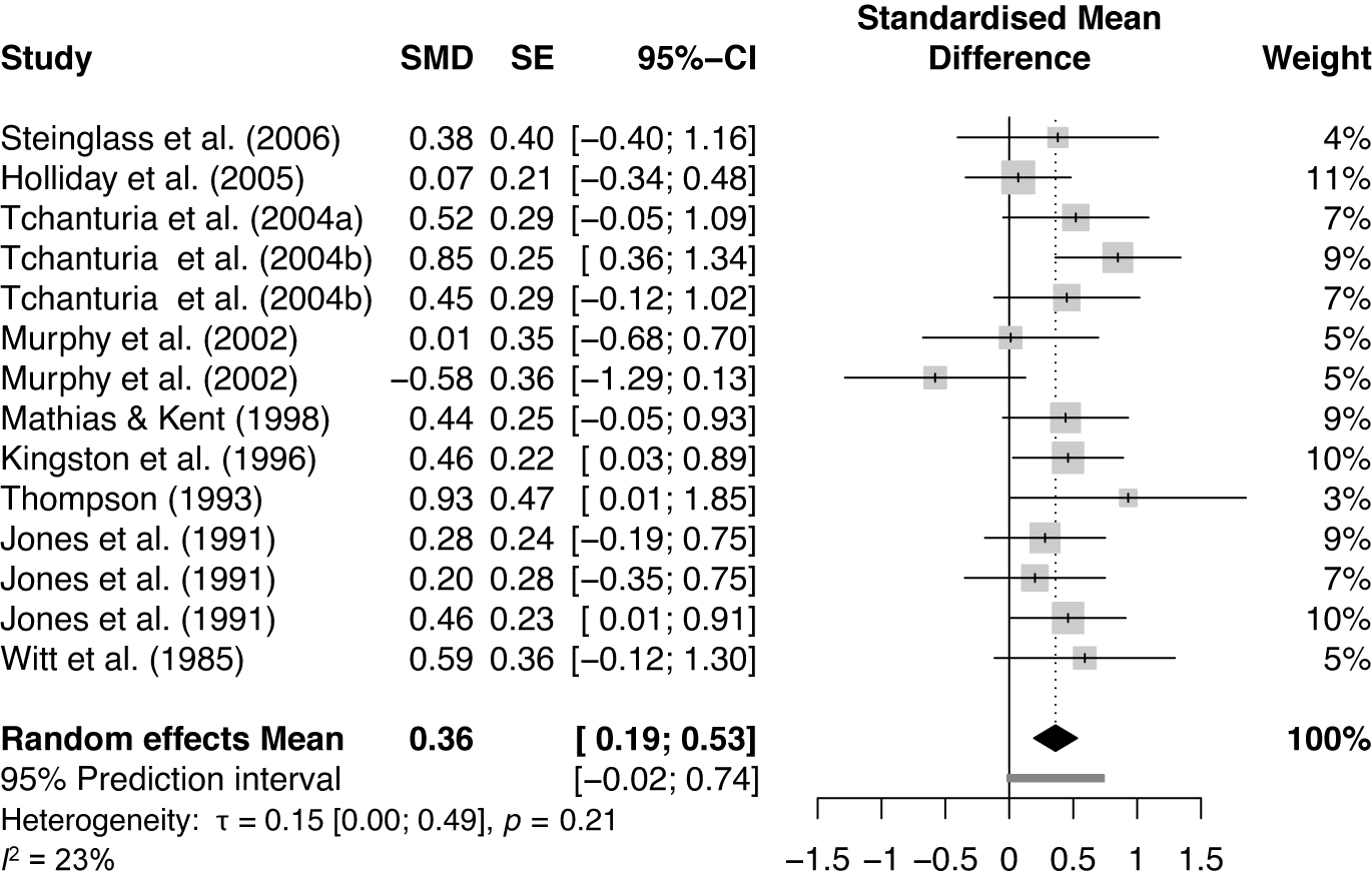
Roberts et al.Reference Higgins, Thompson and Spiegelhalter^2, Reference Roberts, Tchanturia, Stahl, Southgate and Treasure¹² performed meta-analysis on 14 studies comparing the time to complete a trail making task between people with eating disorders and healthy controls. They calculated SMDs (Cohen’s d) and considered these effect sizes negligible if $\geq -0.15$ and $<0.15$ , small if $\geq 0.15$ and $<0.40$ , medium if $\geq 0.40$ and $<0.75$ , large if $\geq 0.75$ and $<1.10$ , very large if $\geq 1.10$ and $<1.45,$ and huge if $\geq 1.45$ . We performed a random-effects meta-analysis on the data and produced a forest plot showing an estimate and 95% CI for $\tau $ (Figure 1).

Figure 1 Random-effects meta-analysis comparing the time to complete a trail making task in people with eating disorders and healthy controls.Reference Higgins, Thompson and Spiegelhalter^2, Reference Roberts, Tchanturia, Stahl, Southgate and Treasure¹² DerSimonian and Laird estimator of $\tau $ used. Figure produced using the R package meta.

In this example, the mean [95% CI] of the modeled distribution of true SMDs was estimated to be $\widehat {\mu }=0.36 \ [0.19, 0.53]$ . The estimated SD of that distribution was $\widehat {\tau }=0.15$ , which corresponds to a 68% range of $[\mu - 0.15, \mu + 0.15]$ and a 95% range of $[\mu - 0.30, \mu + 0.30]$ when a normal distribution is assumed. For example, if $\mu $ was 0.35, then the 68% range would be $[0.2,0.5]$ and the 95% range would be $[0.05,0.65]$ . We view this as a substantial amount of heterogeneity in this context. The 95% CIReference Viechtbauer¹ for $\tau $ was [0, 0.49], indicating that a degenerate distribution (homogeneity) is possible, as is a distribution with a huge SD (if $\tau =0.49,$ then the 95% range is $[\mu - 0.98, \mu + 0.98]$ ). It is clear that there is considerable uncertainty in the SD of this distribution. These interpretations are readily apparent because an estimate and CI for $\tau $ were reported. This provides a more informative and nuanced understanding than a binary statement, such as “heterogeneity was present ( $\widehat {\tau }>0$ )” or “no evidence of heterogeneity was found ( $p=0.21$ ).”

3.2 Ratios

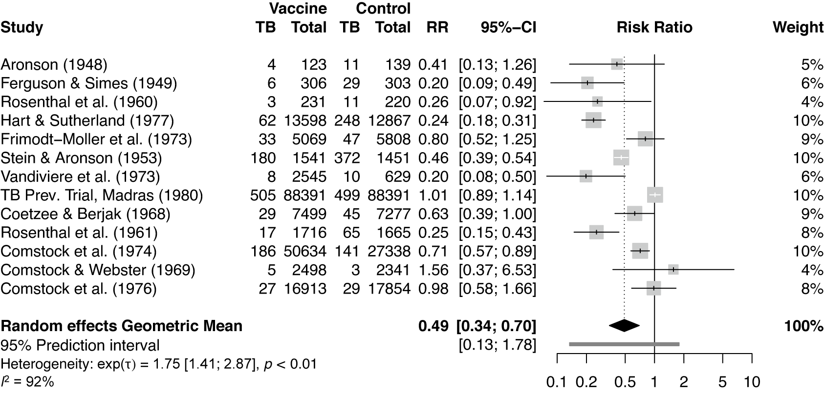
The bacille Calmette–Guérin (BCG) vaccine is used to prevent tuberculosis. Colditz et al.Reference Colditz, Brewer and Berkey¹³ performed a meta-analysis on the efficacy of the vaccine using RRs from 13 randomized trials. We performed a random-effects meta-analysis on the data and produced a forest plot showing an estimate and 95% CI for $\exp (\tau )$ (Figure 2).

Figure 2 Random-effects meta-analysis comparing the risk of tuberculosis (TB) between vaccine and control groups.Reference Colditz, Brewer and Berkey¹³ REML estimator of $\tau $ used. Figure produced using the R package meta with some manual editing.

The GM [95% CI] of the modeled distribution of true RRs was estimated to be $\widehat {{\mathrm {{GM}}}} = 0.49 \ [0.34, 0.70]$ . The estimated geometric SD was $\exp (\widehat {\tau })=1.75$ , which corresponds to a 68% range of $[{\mathrm {{GM}}} / 1.75, {\mathrm {{GM}}} \times 1.75]$ and a 95% range of $[{\mathrm {{GM}}} / 1.75^2, {\mathrm {{GM}}} \times 1.75^2] = [{\mathrm {{GM}}} / 3.06, {\mathrm {{GM}}} \times 3.06]$ when a lognormal distribution is assumed. For example, if the $\mathrm {{GM}}$ was 0.5, then the 68% range would be $[0.29,0.88]$ and the 95% range would be $[0.16,1.53]$ . We interpret this as considerable heterogeneity in the true RRs between trials. Repeating the process with the lower bound of the 95% CIReference Viechtbauer¹ for $\exp (\tau )$ (i.e., 1.41), if the $\mathrm {{GM}}$ was 0.5, then the 68% range would be $[0.35,0.71]$ and the 95% range would be $[0.25,0.99]$ . These calculations are straightforward because an estimate and CI of $\exp (\tau )$ were reported. Clearly, there is much heterogeneity here. This is more informative than a binary statement, such as “heterogeneity was present ( $\widehat {\tau }>0$ )” or “evidence of heterogeneity was found ( $p<0.01$ ).”