





1 Introduction
Mass losses by glaciers and ice caps (henceforth, glaciers) are projected to account for 79–157 mm of global mean sea-level rise (SLR) to the end of the 21st century, depending on the emission scenario (Huss and Hock, Reference Huss and Hock2015). Between 10 and 30% of these glacier mass losses correspond to frontal ablation, dominated by calving and submarine melting in regions such as peripheral Antarctica, Svalbard and the Russian Arctic (Huss and Hock, Reference Huss and Hock2015; Hanna and others, Reference Hanna2020). Although the global glacier volume is only ~0.6% of the ice-sheet volume (Greenland and Antarctica), current glacier contribution to SLR is close to that of the ice sheets (IPCC, Reference Pörtner, Roberts, Masson-Delmotte, Zhai, Poloczanska, Mintenbeck, Tignor, Alegría, Nicolai, Okem, Petzold, Rama and Weyer2019), primarily due to the high sensitivity of glaciers to atmospheric and oceanic forcing (Rignot and others, Reference Rignot, Koppes and Velicogna2010; Motyka and others, Reference Motyka, Dryer, Amundson, Truffer and Fahnestock2013; Straneo and Heimbach, Reference Straneo and Heimbach2013; Luckman and others, Reference Luckman2015; Holmes and others, Reference Holmes, Kirchner, Kuttenkeuler, Krützfeldt and Noormets2019). Beyond the SLR issue, the fresh water input from glacier wastage generates considerable changes in fjord stratification (De Andrés and others, Reference De Andrés2020) and sediment distribution (Mugford and Dowdeswell, Reference Mugford and Dowdeswell2011; Overeem and others, Reference Overeem2017), affecting surrounding marine ecosystems (Meire and others, Reference Meire2017; Hopwood and others, Reference Hopwood2018; Oliver and others, Reference Oliver2018), atmospheric CO2 intakes (Meire and others, Reference Meire2015) and regional ocean circulation (Bamber and others, Reference Bamber2018; Oliver and others, Reference Oliver2018). Thus, studying processes occurring at the glacier–fjord interface is key to understand ongoing changes and generating future projections.
One of the key processes favouring submarine melting at tidewater glacier fronts and driving fresh water export from fjords is the presence of buoyant plumes. Buoyant plumes are primarily driven by subglacial discharge of surface meltwater (SMW) through localised channels at the grounding line, so this process is mostly limited to the melting period in the Arctic (Motyka and others, Reference Motyka, Dryer, Amundson, Truffer and Fahnestock2013; Schild and others, Reference Schild, Hawley and Morriss2016; De Andrés and others, Reference De Andrés2020). These plumes carry sediment from the glacier–fjord bottom towards the surface, and at times become visible at the fjord surface as patches of turbid water (Mankoff and others, Reference Mankoff2016; How and others, Reference How2019; De Andrés and others, Reference De Andrés2020). As the plumes rise, they entrain large volumes of ambient fjord waters, increasing their initial volume by more than an order of magnitude (Mortensen and others, Reference Mortensen2013; Mankoff and others, Reference Mankoff2016) and acting as the engine of convection-driven circulation in the fjords (Motyka and others, Reference Motyka, Dryer, Amundson, Truffer and Fahnestock2013; De Andrés and others, Reference De Andrés2018), thus favouring the input of warmer ocean waters (Straneo and others, Reference Straneo2011). Due to their turbulent nature, the buoyant plumes enable ocean heat transfer to the ice, enhancing submarine glacier-front melting (Sciascia and others, Reference Sciascia, Straneo, Cenedese and Heimbach2013; Xu and others, Reference Xu, Rignot, Fenty, Menemenlis and Flexas2013; Kimura and others, Reference Kimura, Holland, Jenkins and Piggott2014; Slater and others, Reference Slater, Nienow, Cowton, Goldberg and Sole2015, Reference Slater2018). In addition, submarine melting results in a change of shape of the submerged part of the glacier front that has an impact on calving rates (O'Leary and Christoffersen, Reference O'Leary and Christoffersen2013; Luckman and others, Reference Luckman2015; De Andrés and others, Reference De Andrés2018; Schild and others, Reference Schild2018; Vallot and others, Reference Vallot2018; How and others, Reference How2019) by altering the glacier stress field near the terminus (Ma and Bassis, Reference Ma and Bassis2019), likely amplifying the total frontal ablation of tidewater glaciers.
A great scientific effort has been made during recent years to improve our understanding of the glacier–fjord system interactions. Apart from observational improvements, we focus here on modelling these glacier–fjord interactions. Recent glacier–fjord coupled models have shown that submarine melting is amplified by buoyant plumes (Cook and others, Reference Cook, Christoffersen, Todd, Slater and Chauché2020), being a key process to reproduce the observed calving rates and glacier front position changes (De Andrés and others, Reference De Andrés2018; Vallot and others, Reference Vallot2018). However, due to the turbulent nature of the buoyant plumes, high-resolution model grids are needed next to the glacier front to realistically simulate glacier–fjord heat exchange, which involves a huge computational cost when running general circulation models (GCMs) such as MITgcm. If we aim at simulating future projections, we do need to build-up more computationally efficient models. A suitable option to reduce the computational cost would be to build-up a half-cone plume model nested within a low-resolution fjord model. The conditions derived from the plume model would be used as boundary conditions for the fjord and vice versa (Cowton and others, Reference Cowton2016). Nevertheless, recent findings suggest that subglacial discharge channels could be not as spatially localised as previously thought, but could instead be more widely distributed along the grounding line (Fried and others, Reference Fried2015, Reference Fried2019; Sutherland and others, Reference Sutherland2019). Further recent studies also suggest that the truncated line plume model is the most appropriate for plumes developed at tidewater glacier fronts (Jackson and others, Reference Jackson2017; De Andrés and others, Reference De Andrés2020). The line plume model is originally based on the 1-D formulation of Jenkins (Reference Jenkins2011) and is uniformly distributed across the channel width. The computational requirements of the line plume model are low compared with GCMs (as will be shown later), which makes it suitable for long-term simulations and future projections. Idealised simulations of a 1-D coupled flowline–plume model have already been used to study the effects of subglacial topography on submarine ice-front melting (Amundson and Carroll, Reference Amundson and Carroll2018), and provided more realistic simulations that have allowed analysing the response of Greenland outlet glaciers to global warming (Beckmann and others, Reference Beckmann2019).
Here, we build-up a 2-D glacier–line–plume coupled model that includes subglacial discharge, submarine melting and iceberg calving. We simulate the response of Hansbreen glacier, in SW Svalbard, during 5 months within the melt season (April–August) of 2010, and compare the results with those from a coupled glacier–fjord–circulation model (De Andrés and others, Reference De Andrés2018), both models being constrained by the same observational dataset. In particular, we analyse the differences in submarine melting and resulting frontal shapes, net-stress fields within the glacier front, cumulative calving and front position changes produced when using each model. We analyse the glacier–plume model performance and computational efficiency to evaluate its suitability as a tool for long-term simulations.
2 Methods
2.1 Study area and data
Hansbreen Glacier–Hansbukta Fjord system is a branch of the Hornsund fjord, in South–West Spitsbergen, Svalbard, at ~77°N (Fig. 1a). Hansbreen is a tidewater glacier about 16 km long and 2.5 km wide. It has a 1.5 km wide calving front, with a vertical face that is ~100 m thick at the central flowline, of which 50–60 m are submerged. Surface velocity increases towards the terminus, reaching values up to ~7 m week−1 (Fig. 1b). Iceberg calving usually starts in May and ends in October, showing a mean annual calving rate of about 250 m a−1 between 1989 and 2000 (Blaszczyk and others, Reference Blaszczyk, Jania and Hagen2009). Hansbukta is a ~2 km long and shallow fjord (<80 m in depth), with water depth close to the central part of the glacier front of ~55–57 m.
(a) Hansbreen–Hansbukta system, Svalbard (inset), displayed on an ASTER image in universal transverse mercator coordinates (m) for zone 33X. The white triangle represents the position of a time-lapse camera used to measure front position. The modelled flowline is defined by the red line (extended into Hansbukta) and blue dots indicate the locations of the stakes for velocity measurements (orange dots are not used in our analysis). Yellow circles in Hansbukta indicate the location of the CTD stations (~300 m from front) used to provide ambient fjord–water properties; time evolution of (b) ice surface velocities, increasing towards the terminus and measured at the blue stakes in a); (c) SMW estimates (blue line) and ice mélange cover (red line; F: free; P: partial; C: complete); and (d) temperature and (e) salinity profiles in Hansbukta (measured at yellow CTD stations in a), from 1 April to 9 August 2010, coincident with the yellow region in (b) and (c). Coloured lines represent observations. Grey lines are interpolations, showing a continuous warming (freshening) in temperature (salinity) with time.
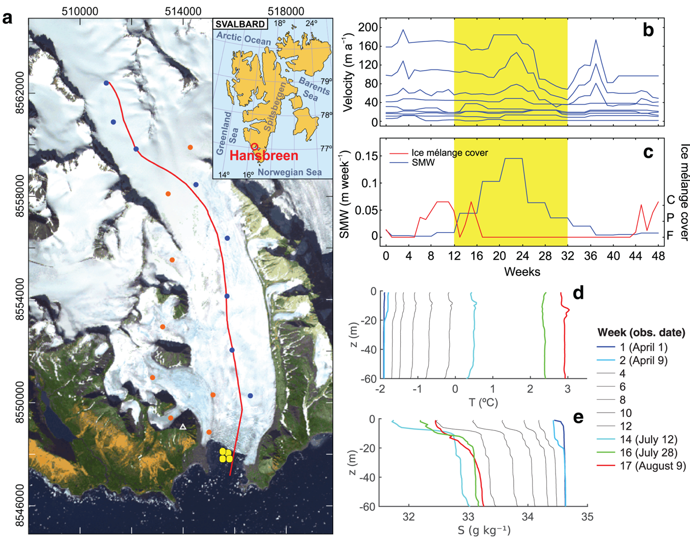
Observational input data to the glacier model include surface velocities, front positions, ice mélange coverage, surface elevation, bedrock topography and surface mass balance (SMB). Ice surface velocities (Fig. 1b) were measured daily, from May 2005 to April 2011, at stakes located close to the flowline (Puczko, Reference Puczko2012) and from terrestrial laser scanner for the velocities at the glacier terminus (data generously provided by Jacek Jania (University of Silesia) from surveying and data processing by Jacek Krawiec (Laser 3-D), Artur Adamek (Warsaw University of Technology) and Jacek Jania). Front position data and ice mélange coverage from time-lapse camera images taken every 3 hours (Fig. 1c) were processed and averaged over weekly intervals between December 2009 and September 2011 (Otero and others, Reference Otero2017). SMB was obtained from European Arctic Reanalysis data, with 2 km horizontal resolution and hourly temporal resolution, constrained by automatic weather stations and stake observations (Finkelnburg, Reference Finkelnburg2013). Mean SMB and SMW at each flowline point were calculated by applying bilinear interpolation to the available 2-km resolution hourly accumulation and ablation data (Fig. 1c). The surface elevation came from the SPIRIT digital elevation model for gentle slopes, with a 30 m RMS absolute horizontal precision and 40 m resolution. Bedrock topography was inferred from the ground-penetrating radar data (Grabiec and others, Reference Grabiec, Jania, Puczko, Kolondra and Budzik2012; Navarro and others, Reference Navarro2014).
Available oceanographic data overlap glaciological data only from April to August of 2010, limiting our modelling period to ~20 weeks. Oceanographic data consist of conductivity–temperature–depth (CTD) profiles in Hansbukta (Fig. 1d, e). All the data were vertically averaged every 1 dbar (1 kPa). Data gaps (CTDs for missing weeks) were linearly interpolated, maintaining the vertical structure of the water column (i.e. the interpolation was applied to each vertical level; Fig. 1d, e). Temperature (salinity) in Hansbukta experiences strong seasonal variability, ranging from −1.8 to 3°C (34.6–31.8 g kg−1), from April to August, respectively.
2.2 The coupled glacier–plume model
2.2.1 Glacier dynamics model
We use Elmer/ice (e.g. Gagliardini and others, Reference Gagliardini2013) to model the ice flow, with the 2-D stress and velocity fields being computed along the glacier central flowline.
The Stokes system of equations for an incompressible viscous fluid is used to model the dynamics of glacier ice in 2-D. A body force term is added to the conservation of linear momentum equation to account, in a 2-D model, for friction from the shear margins, assuming a parabolic glacier cross-section (Jay–Allemand and others, Reference Jay-Allemand, Gillet-Chaulet, Gagliardini and Nodet2011). As a constitutive relation, we adopt Nye's generalisation of Glen's flow law. We introduce a fracture-induced softening term to quantify the loss of the load-bearing surface area due to fractures (Borstad and others, Reference Borstad2012). The time evolution of the glacier surface is calculated by solving the free-surface evolution equation that incorporates the flow of ice and the mass balance at the surface.
As boundary conditions, we consider the upper surface of the glacier as a traction-free boundary with no explicit conditions on velocities. At the ice divide, shear stresses and horizontal velocity are set to zero. The space-dependent friction coefficient at the glacier bed is calculated monthly using an inverse Robin method (Arthern and Gudmundsson, Reference Arthern and Gudmundsson2010; Jay–Allemand and others, Reference Jay-Allemand, Gillet-Chaulet, Gagliardini and Nodet2011). At the glacier terminus, we set back stress to zero above sea level and equal to the water depth-dependent hydrostatic pressure below sea level.
Crevasse depth is calculated as the depth at which the longitudinal tensile strain rate tending to open the crevasse equals the creep closure rate resulting from the ice overburden pressure. Calving is assumed to occur when surface crevasses reach the waterline (Benn and others, Reference Benn, Hulton and Mottram2007). The water pressure contributing to crevasse opening is a function of the depth of water filling the crevasse (Dw, in m), which can be considered either as constant or as a function of SMW rate (in m week−1, Fig. 1c), as described in De Andrés and others (Reference De Andrés2018), such that

where Δt g is the glacier-model time step (one week), and f is a non-dimensional adjustable parameter used to parameterise the unknown Dw in terms of the SMW.
The glacier domain is divided into a rectangular mesh with 10 vertical levels and a horizontal grid resolution increasing from ~50 m in the upper glacier up to ~25 m close to the front. At each time step, surface elevations are computed from surface mass–balance estimations and surface velocities, and the grid nodes are shifted vertically to fit the new geometry. At the terminus, the grid nodes are shifted down–glacier according to the velocity vector and the length of the time step, and the terminus position is updated according to the calving criterion. At a given time step, if the glacier front is calved, the model domain is remeshed assuming a vertical ice front. Otherwise, we preserve the shape of the front resulting from submarine melt undercutting.
Prognostic model runs were carried out with a ~1 week (1/48 of a year) time step. Every 4 weeks (four time steps), we ran an initialisation process for the glacier model, which consisted of solving the Robin problem to force a best-fit basal friction coefficient to be used for the subsequent four time steps. This initialisation was done to minimise the misfit between observed and modelled surface velocities.
2.2.2 The line–plume model
The buoyant plume theory is a common tool for estimating submarine front melting and studying the impact of subglacial meltwater discharge on calving rates (Jenkins, Reference Jenkins2011; Carroll and others, Reference Carroll2015, Reference Carroll2016; Slater and others, Reference Slater, Goldberg, Nienow and Cowton2016, Reference Slater2017; De Andrés and others, Reference De Andrés2018; Vallot and others, Reference Vallot2018). Based on the good results from previous studies (e.g. Fried and others, Reference Fried2015; Jackson and others, Reference Jackson2017; De Andrés and others, Reference De Andrés2020), we use here the line plume model of Jenkins (Reference Jenkins2011) slightly modified by Slater and others (Reference Slater, Goldberg, Nienow and Cowton2016, Supplementary Information) to allow, in such a case, the calculation of plume properties beyond its neutral buoyancy and up to its maximum height (for basics see Morton and others, Reference Morton, Taylor and Turner1956; Slater and others, Reference Slater, Goldberg, Nienow and Cowton2016).
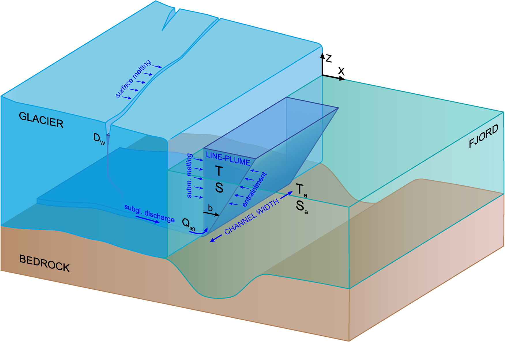
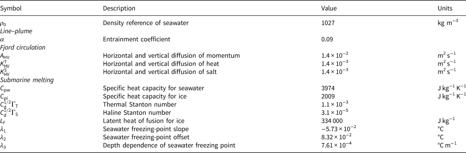
The line–plume model is steady in time and the only independent variable for tidewater glaciers is the vertical dimension, z, so it is strictly a 1-D model that considers constant plume properties along the plume width (i.e. the channel width, see Fig. 2 for schematics on plume geometry and properties). The evolution of the plume properties (thickness, vertical velocity, temperature and salinity) along the vertical tidewater face (z) is described by four ordinary differential equations that conserve the fluxes of mass, momentum, heat and salt. The entrainment rate and the turbulent transfer of heat and salt are all considered as linear functions of the plume velocity, through the entrainment coefficient, α, and the Stanton numbers, $C_d^{1/2} {\rm \Gamma }_{T, S}$ , respectively (see values in Table 1). The plume model is closed using the thermodynamical equation of state (TEOS-10, McDougall and Barker, Reference McDougall and Barker2011) to calculate the plume and ambient densities and the submarine melt model described below, in Section 2.2.4.
Idealised Hansbreen–Hansbukta interface where a schematic of the buoyant line–plume model is represented. Note that the cross-sectional width of the plume is that of the discharging channel. Plume thickness, b, grows towards the fjord surface due to the entrainment of ambient and melt waters. Subglacial discharge intensity (Q sg) and ambient properties, temperature (T a) and salinity (S a), will determine plume thickness and properties (T and S) at a given depth. Also shown in the picture is a crevasse filled by SMW by an amount Dw.
Physical parameters used in the line–plume, fjord circulation and submarine melt models
We assumed a constant subglacial channel of 200 m width, as it was the nominal fjord width obtained in De Andrés and others (Reference De Andrés2018) (see also Section 2.3.1). To initialise the model, we prescribe a subglacial discharge flux, Q sg, across the channel width (Q sg/W) at the grounding line and use the observed temperature and salinity profiles as ambient properties (boundary conditions).
2.2.3 The fjord circulation model
The 2-D fjord circulation model of Hansbukta was thoroughly described in De Andrés and others (Reference De Andrés2018). We include here some details of the model to facilitate the basics for understanding the present work. We used the Boussinesq and non-hydrostatic form of the Massachusetts Institute of Technology general circulation model (MITgcm; Marshall and others, Reference Marshall, Adcroft, Hill, Perelman and Heisey1997) for incompressible and stratified fluid in a non-rotating system.
We set a 2-D fjord domain of ~2 km in length along the x-coordinate (as an extension of the glacier central flowline), varying in size according to changes in glacier front position. The mesh consisted of 200 × 90 cells (horizontal–vertical). To capture the turbulent buoyant plume, we set a high-resolution x-zone of 1 m grid–cell length for the 100 m closest to the glacier front, and then linearly increasing to the end of the domain. The grid–cell height along the z-coordinate was fixed to 1 m. We tested the sensitivity of the model to spatial resolution and constrained viscous and diffusive coefficients based on sensitivity analysis (see values in Table 1 and details in De Andrés and others Reference De Andrés2018). We set a closed seabed boundary following the observed bathymetry with no-slip conditions. The glacier front (left side of the fjord domain) was also considered as a permanently vertical closed boundary with no-slip conditions in the fjord model. The fjord mouth was set as an open boundary with transient temperature and salinity profiles according to observed oceanic forcing. We set a time step of 0.5 s. We used the observed temperature and salinity profiles as initial conditions and prescribed them along the entire horizontal grid (horizontally uniform). The velocity fields reached at the end of every one-week period were set as initial conditions for the subsequent step to maintain the continuity of the modelled water circulation patterns. A spin-up period of 1 week was run in a standalone ocean configuration to get initial velocity fields for the first fjord circulation period. The model was reinitialised every week to get a glacier-model feedback (updated geometry).
We introduced Q sg by constantly adding fresh water at the local freezing-point temperature, through one cell located at the glacier front grounding point and considering a nominal fjord width of 200 m (Q sg/W). The added fresh water mass was balanced by prescribed barotropic velocities across the open boundary (Cowton and others, Reference Cowton2016).
2.2.4 The submarine melt model and the coupling mechanism
Both fjord–circulation and line–plume models use the three thermodynamic–equilibrium equations at the ice–ocean interface (Holland and Jenkins, Reference Holland and Jenkins1999) to estimate the submarine melt rates (SMRs), in m s−1, at a given depth of the calving front. The freezing-point temperature at the boundary depends on local pressure and salinity and the heat and salt budgets at the ice–ocean interface are computed for a given melt rate of ice. The submarine melt model requires constraints on physical parameters, which can be found in Table 1. The parameter values that we used here were those recommended for ice sheets (Jenkins and others, Reference Jenkins, Nicholls and Corr2010). Despite these values still need validation against observations for tidewater glaciers, they have been widely used in the literature for modelling submarine melting in tidewater glaciers (Sciascia and others, Reference Sciascia, Straneo, Cenedese and Heimbach2013; Slater and others, Reference Slater, Nienow, Cowton, Goldberg and Sole2015, Reference Slater, Goldberg, Nienow and Cowton2016; Mankoff and others, Reference Mankoff2016; Cook and others, Reference Cook, Christoffersen, Todd, Slater and Chauché2020).
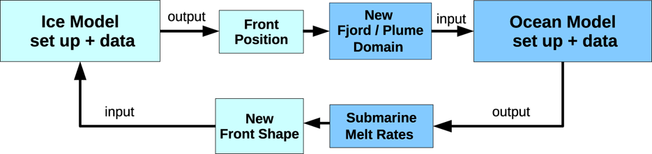
Coupling between our glacier and plume (or fjord) models is accomplished through two main mechanisms: (1) depth-dependent SMRs are weekly calculated (SMR)) by both the plume and the fjord circulation models and used to modify the shape and domain of the submerged part of the modelled Hansbreen's front. These modifications likely affect the stress regime calculated by the model; (2) the movement (advances/retreats) of the glacier front over the fjord bottom defines the depth of the submerged part of the front every week, implying changes in the flotation conditions. From the ocean-model (plume or fjord) perspective, the submerged ice front (left fjord boundary) is assumed to remain vertical at any time (even in the absence of iceberg calving). We feel confident with this choice since, according to the subglacial discharge fluxes and glacier front shapes in our experiments, changes in ice-front shape do not have a significant effect on plume dynamics or SMRs (Slater and others, Reference Slater2017). Both ice and ocean models run asynchronously and automatically, exchanging information every modelled week, according to the glacier-model time step. The total modelled time was 20 weeks: 17 weeks constrained by CTD observations (from 1 April 1 to 9 August 2010, interpolated when data were not available) plus 3 additional weeks based on temperature mooring data (De Andrés and others, Reference De Andrés2018, Supplementary Information).
2.3 Experiments
We here analyse the differences between the coupled glacier–fjord and glacier–plume models in different experiments. To compare the results from both models, all the experiments performed here follow the same design as in a previous work (De Andrés and others, Reference De Andrés2018). Note that both models were run under weekly forcings. Therefore, giving the steady-state nature of the plume model, there is just a weekly estimation of SMRs. The transient fjord model, however, allows us to estimate weekly SMRs based on daily calculations. With our experimental design, our results do not provide information on the differences in submarine melting under equal conditions (which has been already addressed, e.g. Carroll and others, Reference Carroll2015), but on what each model is capable of representing under equal forcing conditions, and its effects in terms of calving rates and front position changes.
2.3.1 Sensitivity of submarine melting to subglacial discharge
In this experiment, we test how the modelled SMRs at the glacier front would change under different configurations of Q sg/W. For these simulations, we run the coupled model with Dw = 0.
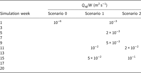
While observations of subglacial discharge rates are seldom available, it has been shown that, from a certain threshold value, subglacial discharge plays a fundamental role in amplifying SMRs (Beckmann and others, Reference Beckmann, Perrette and Ganopolski2018). To tune the discharging fluxes, De Andrés and others (Reference De Andrés2018) resolved the circulation in Hansbukta with different Q sg/W (constrained by SMW, Fig. 1c) while considering a unique channel. The best-fit Q sg/W was inversely inferred from fjord properties every simulated week from April to August of 2010. The inference was based on a criterion of best fit between observed and modelled fjord temperature while keeping a fair match with salinity observations. After obtaining the best-fit Q sg/W for each modelled week, assuming a single discharging channel in Hansbukta and considering SMW constraints, a nominal fjord width (channel width) of 200 m was suggested. Here, we use the same Q sg/W values used in De Andrés and others (Reference De Andrés2018), which can also be found in Table 2.
Time series of subglacial discharge fluxes implemented across the 200 m channel width (Q sg/W) in the different scenarios described in the text
Despite having already available the best-fit Q sg/W values, we here perform additional simulations with Q sg/W values lower (near zero) and higher (double) than those resulting from the best fit, to obtain information about our model performance and the sensitivity of submarine melting to subglacial discharge intensity.
Scenario 0: Q sg/W is assumed to be near zero (10−6 m3 s−1, as we need it to be non-zero to initialise the line–plume model) during the entire 20-week simulation (Table 2). This allows us to analyse how submarine melting would evolve throughout the summer in the absence of turbulent buoyant plumes (though weak laminar plumes are potentially formed as submerged ice melts), thus showing the effect of ocean thermal forcing alone.
Scenario 1: It represents the best-fit Q sg/W scenario obtained in the subglacial–discharge–tuning experiment of De Andrés and others (Reference De Andrés2018), so it can be considered as the most realistic scenario for our coupled model (see values of Q sg/W in Table 2). Scenario 1 is also used to test the influence that submarine melting exerts on glacier front dynamics (see the next experiment).
Scenario 2: In this scenario, Q sg/W values are the same as in Scenario 1 for weeks 1–12, and then are doubled to the end of the modelling period (Table 2). This shift in Q sg/W represents possible sudden discharge events associated with more intense surface melting episodes not registered by our observations, and allows us to analyse the impact of the subsequent submarine ice melting on calving.
2.3.2 Sensitivity of front position and calving rates to submarine melting and crevasse water depth
Here, we focus on two mechanisms controlling calving rates and front position changes during the summer: SMRs (Morlighem and others, Reference Morlighem2016; Seroussi and others, Reference Seroussi2017) and crevasse water depth (Dw) (Cook and others, Reference Cook, Zwinger, Rutt, O'Neel and Murray2012; Otero and others, Reference Otero2017; De Andrés and others, Reference De Andrés2018). First, we analyse the contribution of SMR alone to calving and front position changes. We use the three different scenarios of subglacial discharge described above, while maintaining Dw equal to zero. Second, to evaluate the contribution of Dw to calving and front position changes we run the coupled model maintaining fixed the SMR scenario. We use the best-fit SMR scenario (Scenario 1) and perform several runs varying Dw in two ways: (i) applying constant values of Dw = 0, 2, 3 m; and (ii) considering surface–meltwater–dependent Dw (Eqn (1)), with f = 75, 100, 130. This experiment allow us to determine which configuration produces the best fit between modelled and observed front position changes, and the relative importance of each mechanism in controlling calving and/or front position.
2.3.3 Comparison between glacier–fjord and glacier–plume coupled models
In this experiment, we focus on the different results obtained from the two coupled models. Once the configuration that best matches the observed front positions is established, we compare how the submerged ice-front melting evolves throughout the summer for both coupled models: the glacier–plume and the glacier–fjord. In addition, we estimate the weekly vertically integrated ablation due to submarine melting calculated with each model. We also study the shape of the submerged part of the front resulting from melting for each model, trying to establish patterns of ‘characteristic profiles’. Finally, we analyse how these characteristic profiles affect the net-stress field near the glacier front and their implications on calving rates and front position.
3 Results
3.1 Submarine front melting under different subglacial discharge scenarios without water in crevasses
A common characteristic of the three scenarios, for both models, is that SMR increases as summer progresses (Fig. 4), becoming maximum in week 17. As there is almost null discharge in Scenario 0, we can interpret that part of this increase in submarine melting is due to warmer fjord waters as summer progresses (Fig. 1d). For scenarios 1 and 2, Q sg becomes higher throughout the simulation period (Table 2), making its own contribution to the increase in submarine melting. In case of Scenario 1, SMR is higher than that of Scenario 0, but lower than SMR obtained in Scenario 2. Therefore, we can attribute this submarine melt enhancement among scenarios to the increase in Q sg. However, SMR following week 17 drops slightly in the plume model, while it remains at its maximum level in the fjord model. Another characteristic common to the three scenarios, despite having different discharge fluxes, is that the SMR produced until week 7 is <1 m week−1, which is similar in both models and is consistent with the low Q sg/W (≤0.002 m3 s−1, see Table 2) and with the ambient temperature (<−1°C) during these weeks (see Fig. 1d). An important aspect is that, in the plume model, maximum SMR takes place at the fjord surface (Fig. 4a), except for the first weeks of Scenario 0, when the maximum SMR occurs at intermediate depths, between 16 and 27 m (it is not evident in Fig. 4a, but it is clearly seen from the numerical results). Having in mind that temperature profiles in Hansbukta are vertically quasi-homogeneous (Fig. 1d), the fact that maximum SMR occurs in the vicinity of sea level is the result of plume velocities and temperatures being highest at that level (e.g. ~0.53 m s−1 and 2.8°C, respectively, in week 16 of Scenario 1). Maximum plume velocities at the fjord surface imply that the plume has not reached its neutral buoyancy yet (discussed in Section 4.4). This aspect differs from the results obtained with the fjord model, in which the melting profile indicates that the maximum SMR occurs at intermediate depths, at ~30 m (Fig. 4a), where velocities and temperatures reach, for example, 0.55 m s−1 and 2.6°C, respectively, in week 17 under Scenario 1.
Workflow diagram of the different components in the coupled model. The ocean model here represents either component, the line–plume or the fjord circulation model.
Time evolution of weekly SMRs estimated with (a) the glacier–plume and (b) the glacier–fjord models, both with no water in crevasses. Three different scenarios are considered for each model, ranging from almost–null subglacial discharge in Scenario 0 to amplified discharges towards Scenario 2 (see Table 2). The submerged part of the ice front (all the coloured parts of the panels) increases with time, as a consequence of Hansbreen advance towards Hansbukta basin.
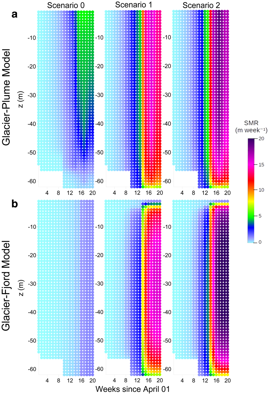
Analysing the scenarios separately we obtain that maximum SMR under Scenario 0 of the plume model (Fig. 4a) varies from 4 × 10⁻³ m week−1 in April to ~5 m week−1 in August, i.e. an increase by three orders of magnitude. Therefore, even in the absence of subglacial discharge the heating experienced by the fjord as the summer advances has a significant effect on the submarine frontal melting. This characteristic is common to the fjord model (Fig. 4b), although the maximum SMR for the latter is lower, ~2 m week−1.
Scenarios 1 and 2 of the plume model share the same discharge from week 1 (beginning of April) to week 11 (end of June), and both produce maximum SMR from ~0.1 m week−1 in April to ~3 m week−1 at the end of June. In the case of the fjord model, the maximum SMR between weeks 1 and 11 is lower (there is even refreezing), ranging from ~0.01 m week−1 in April to ~2 m week−1 at the end of June. That is, the relative differences in maximum SMR between both models are larger in the first week, by ~90%, becoming smaller as they approach week 11, when the relative difference between maximum SMR is reduced to 33%.
From week 11, Scenarios 1 and 2 differ in their SMR. In Scenario 1 of the plume model (fjord model) maximum SMR of ~4 (2.5) m week−1 is obtained in week 12−early July−and ~16 (16) m week−1 during weeks 17 and 18−middle August. Corresponding values for the maximum SMR of the plume model (fjord model) for Scenario 2 are ~4.5 (3.5) m week−1 at the beginning of July and ~19 (21) m week−1 in the middle of August. In both scenarios, the relative differences between the maximum SMR obtained with both models is reduced as the summer progresses up to week 17 (SMR differences are minimum), then starting to grow again, but with maximum SMR higher for the fjord model.
3.2 Evolution of the front position under different configurations of submarine melting and crevasse water depth
In the absence of water in crevasses, both the glacier–plume (Fig. 5a) and the glacier–fjord models (Fig. 5b) exhibit a similar pattern of the continuous advance of the glacier front and no calving events under Scenario 0 of melting. Both models show discontinuous progress under Scenarios 1 and 2 of melting (due to calving events taking place in late summer), indicating that stronger subglacial discharge might lead to more calving. However, there is no difference in cumulative calving between Scenarios 1 and 2 in the glacier–plume model, while a difference is observed in the glacier–fjord model (Fig. 5c). In Scenarios 1 and 2, the first calving event occurs 1 week earlier (week 14) in the plume model compared with the fjord model (week 15). The total frontal ablation over the summer due to calving, under Scenario 1 (Scenario 2), amounts to ~32 (30) m in the plume model, while for the fjord model it is ~17 (32) m (Fig. 5c). This might indicate that higher submarine melting in the fjord model amplifies the instability of the glacier front, promoting more calving. Overall, the three melting scenarios tested in our experiment predict glacier front positions more advanced than those observed, which means that submarine melting alone is not able to reproduce the observed front position.
Time evolution of Hansbreen front position and cumulative calving (right panels) resulting from the glacier–fjord (middle panels) and glacier–plume (left panels) models: (a)–(c) the model run with no influence of crevasse water pressure (Dw = 0 m) and assuming three different scenarios of submarine melting (shown in Fig. 4); (d)–(f) submarine melting of Scenario 1 (best fit) and three different values of Dw (0, 2, 3 m); (g)–(i) the model also runs with Scenario 1 of melting, but Dw is now a function of surface melting (Eqn (1)), with f-ratios of 75, 100 and 130. Observed front positions are represented with black dots.
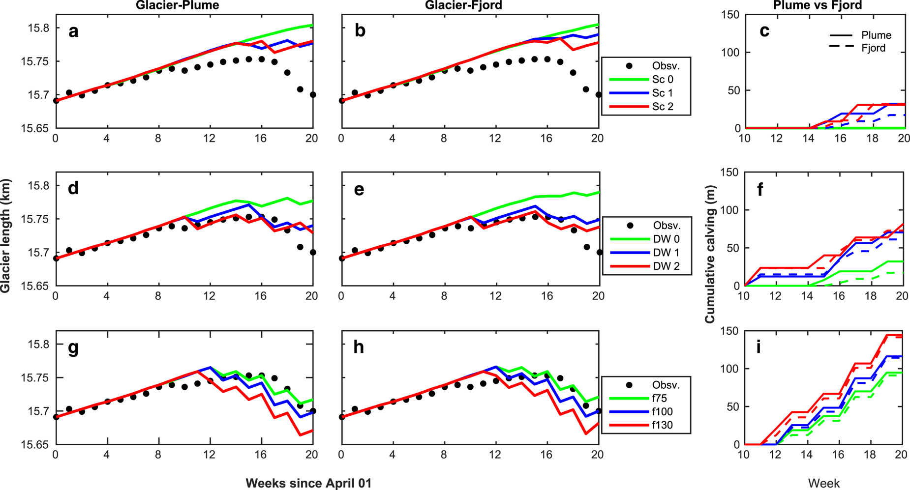
Keeping fixed the more realistic melting scenario of subglacial discharge (Scenario 1 of melting), we analyse the effect that different values of Dw (0, 2, and 3 m, kept constant throughout the simulation period) have on the front position for the glacier–plume (Fig. 5d) and glacier–fjord (Fig. 5e) coupled models. The most evident feature in both cases is the positive relationship between Dw and calving. With Dw ≠ 0, the first calving event occurs between weeks 10 and 11 in both models, but for Dw = 2 m (Dw = 3 m), the plume model accumulates a total of ~70 (82) m of calving, higher than the 62 (73) m obtained with the fjord model (Fig. 5f). With identical configurations, both models predict very similar front positions. In both models, the best-fit corresponds to Dw = 2 m, with a RMSE with respect to observations of ~12 m.
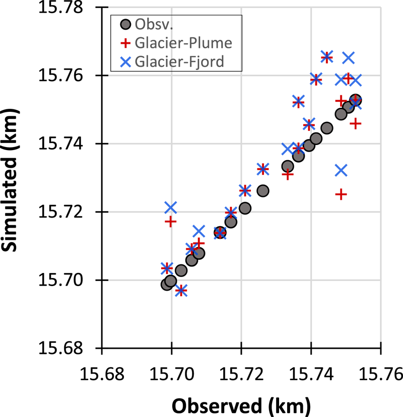
In a second experiment, we set Dw as proportional to the surface melting throughout the summer, i.e. Dw ∝ f ⋅ SMW (Eqn (1), Fig. 1c), and analyse the sensitivity of the front position to parameter f under melting Scenario 1. In Figs 5g, h, we present the front positions of Hansbreen obtained with the glacier–plume and the glacier–fjord models, respectively, for f = 75, 100, 130. As in the previous experiment, a positive relationship between Dw and calving rates is observed (Fig. 5i), though in this case as a function of parameter f. In the glacier–plume model, the first significant calving event occurs at week 11 for f = 100 and 130, and at week 12 for f = 75. These first calving events coincide with those of the glacier–fjord model, except for f = 100, whose first event takes place on week 12. However, none of the two models is able to capture the first observed calving event in week 10, as it was predicted when fixing Dw = 2, 3. The cumulative calving in the glacier–plume (glacier–fjord) model over the entire simulated period is 94 (91) m for f = 75, 116 (114) m for f = 100 and 144 (141) m for f = 130 (Fig. 5i). These results indicate that the submarine melting generated by the plume model has a similar effect on calving than that resulting from the fjord circulation model. The best-fit configuration in both coupled models is that of Scenario 1 of melting and f = 75, for which the RMSE with respect to the observed front position is of ~10 m in both cases. In fact, the squared errors of the two models (under the best-fit configuration) calculated every week show similar deviations with respect to observations (Fig. 6). Overall, both best-fit model predictions overestimate the glacier front position (more advanced than observed), although larger deviations concentrate within weeks 10–12, with longer observed glacier lengths (Fig. 6), corresponding to the middle–end of June 2010. Such deviations coincide with the first and isolated retreat event observed, which is not reproduced at all by any model or scenario. In fact, the first simulated retreat actually occurs from week 12 to 13 for both models under the best-fit configuration. In the glacier–plume model, however, the largest deviation from observations is of 25 m and takes place on week 17 (see Fig. 5), when the glacier front starts an uninterrupted retreat. This differs from the glacier–fjord model, where the maximum deviation of 21 m occurs at the end of the simulation period (week 20), when the glacier has already retreated close to its initial position.
Model residuals. Simulated vs observed front positions (glacier length) of the best-fit configuration (Scenario 1 of submarine melting and factor f = 75 for crevasse water depth) resulting from the glacier–plume (red crosses) and the glacier–fjord (blue blades) models.
3.3 Submarine melting, calving and net-stress distribution under the best-fit configuration
The above results show that the configuration that best matches front position observations is that using the Q sg evolution of Scenario 1 and Dw as a function of SMW (Fig. 1c), with f = 75. In terms of submarine melt evolution, we refer to Figure 4, Scenario 1 (and Dw = 0), to see the evolution pattern and weekly SMRs at depth for both models under the best-fit configuration. Here (best-fit configuration), however, the submerged ice front evolves with time but independently of the model used. The ice front is submerged ~56 m in depth from week 2 to week 9. In week 10, the submerged part of Hansbreen front deepens to 64 m, remaining at this level until week 17. During this period (weeks 10–17), ~70% of the front of Hansbreen is submerged, which is the maximum for the modelled period and coincident with the most advanced front position. From week 18 ahead, the front retreats to locations where submerged depths are of 56 m.
A characteristic common to both models is that submarine melting until week 7 is <1 m week−1, which is coincident with low Q sg (≤0.002 m3 s−1, see Table 2) and ambient temperature (<−1°C) during these weeks (see Fig. 1d). As pointed out in Section 3.1, the general pattern is that maximum melt rates in the plume model occur near the fjord surface, differing from those of the fjord model, in which the maximum melting rates occur at intermediate depths, ~30 m (Figs 4, 7). The maximum melting accumulated along the 20-week simulation reaches 118 m in the line–plume model and 108 m in the glacier–fjord model. To analyse in more detail the differences in melting profiles, the weekly results for each model, along the entire simulation period, are shown in Figure 7. For weeks 1 and 2, both models show minimum SMR at the fjord surface and maximum within the 20 m closest to the grounding point (the source of meltwater). These results could be explained by the low temperatures along the entire water column (–1.8°C), which prevent the ice from melting, but with a little momentum at the source (Q sg of 0.001 m3 s−1, see Table 2), which promotes some little melting within the grounding-line vicinity (<0.15 (0.05) m week−1 in the glacier–plume (glacier–fjord) model). Over the following weeks, the profiles for both models evolve towards their own ‘characteristic profile’, which is reached from week ~9 ahead. For the glacier–plume model, this characteristic profile shows the maximum melting at the fjord surface, and the minimum towards the source, at depth. Looking at the profiles of week 14 onwards in Figure 7, we see a quasi-linear and negative relationship between SMRs and depth. The ‘characteristic profile’ of the glacier–fjord model shows its maximum melt rate within the central region of the submerged front (20–30 m depth) and its minimum values at depth and at surface, producing a parabolic shape.
Melting profiles from week 1 to 20 obtained with the glacier–plume (solid line) and glacier–fjord (dashed line) models. Note that, to highlight the different profiles of both models, the scale of the x-axes varies within weeks.
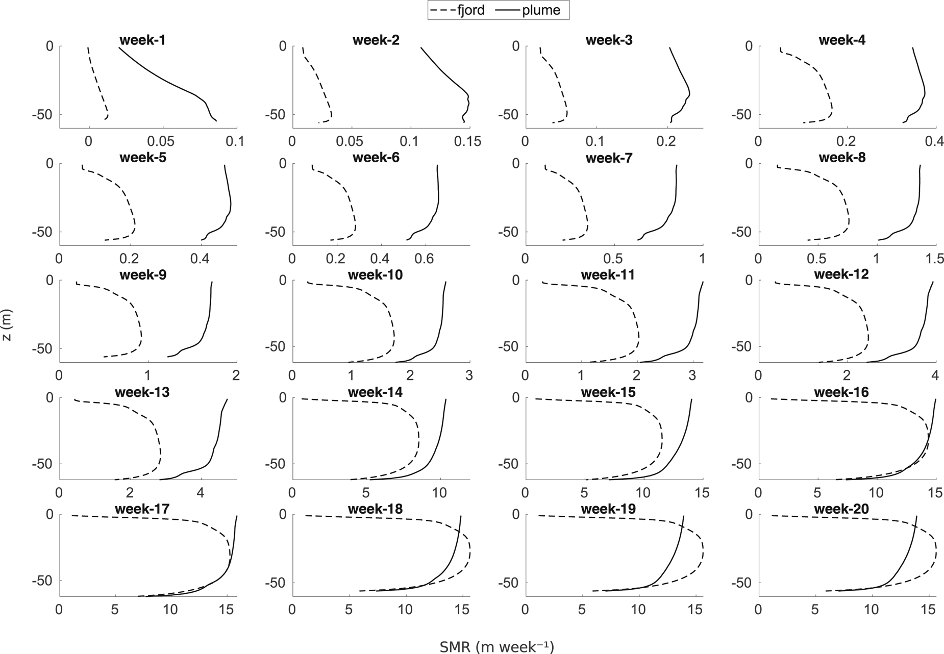
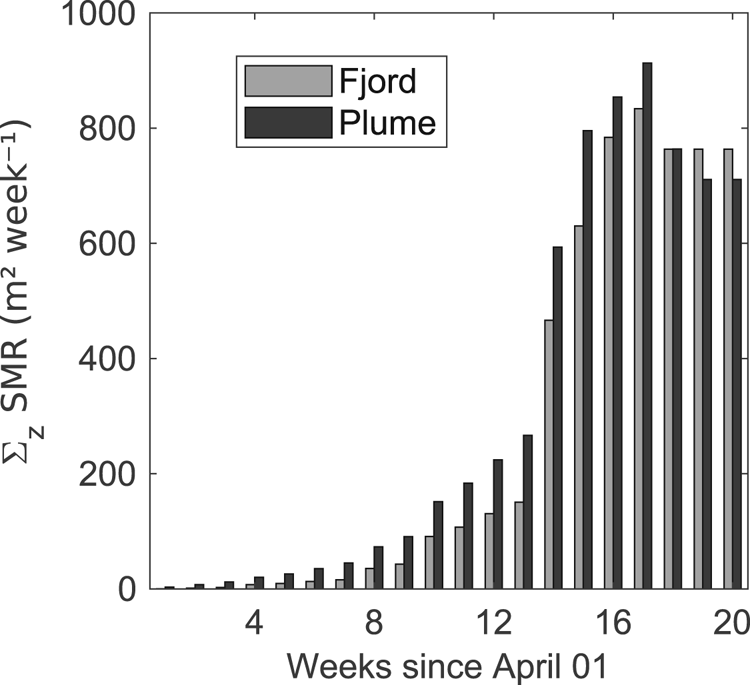
In general, in Figure 7, we observe that the maximum melt rates are higher for the glacier–plume than for the glacier–fjord model, until week 15. During weeks 16 and 17, maximum melt rates are almost equal in both models. Afterwards, they are higher in the fjord than in the plume model. To quantify and analyse the evolution of the total melting experienced by Hansbreen front during each week, we vertically integrate the weekly melt rates and make a comparison between both models (Fig. 8). We verify that the total weekly melting is up to ~30% higher for the plume model than for the fjord model until week 17, when the corresponding SMRs of ~900 and ~850 m2 week−1 are reached. In week 18, submarine melting of both models decreases to ~750 m2 week−1. Thereafter, submarine melting is kept constant for the fjord model, while it decreases to ~700 m2 week−1 in the plume model.
Comparison of the vertically integrated submarine melting obtained with the glacier–plume (dark bars) and glacier–fjord (grey bars) models from week 1 to week 20.
After evaluating the characteristic profiles and mass loss by submarine melting for both models, we study their impact on the stress field near the Hansbreen terminus. As an example, we illustrate in Figure 9 the net-stress fields within the 300 m closest to the glacier terminus, over the last 4 weeks of the simulation period (weeks 17–20). As expected, both models show positive (extensional) net-stress values of up to ~250 kPa at the glacier surface, decreasing to negative values (compressional) of ~−1000 kPa at the bottom. Near the front, different geometric front shapes are found due to submarine melting (weeks 17 and 19, undercutting front profile) and calving (weeks 18 and 20, vertical front profile). In weeks 17 and 19, net stress within the uppermost part of the glacier front is positive in the glacier–fjord model, while it is negative for the glacier plume model, reaching values of ~−250 kPa at the waterline.
Net-stress field distribution along the 300 m nearest to the glacier terminus resulting from simulation weeks 17–20, for (a) the glacier–plume model and (b) the glacier–fjord model. The differences between the net stresses of both models are shown in (c). Ice flow is towards the right, and the 0 of the x-axis is set at the glacier front.

Looking closely at the plume–fjord anomaly (Fig. 9c), we see differences between both models of more than ±50 kPa all along the represented part of the glacier terminus. Focusing on the grid cells immediately close to the front, the glacier–plume model presents net-stress values 50 kPa larger than those of the glacier–fjord model in the uppermost grid cells for weeks 17–19, which could favour calving during that period.
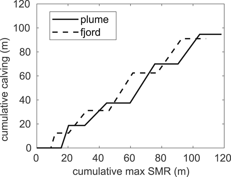
Comparing the trends of cumulative calving and cumulative maximum submarine melting, we see a similar pattern for both models (Fig. 10). The curve follows a discontinuous increase, where the flat segments of the curve correspond to front advances subjected to submarine melting alone. The steps, on the other hand, represent episodes of calving. It seems that melting acts to undercut the front until the undercut section calves off. As described in Section 3.2, the first simulated front retreat corresponds to weeks 12 and 13, accounting for almost 20 (12) m of the calved front in the glacier–plume (–fjord) model, when total maximum submarine melting of ~18 (10) m were already accumulated until that week. These ablation differences between both models become smaller towards the end of the simulation (when differences in the fjord boundary conditions between models are smaller). At the end of the 20-week simulation, the glacier–plume (–fjord) model accumulates total calving and maximum submarine melting of 94 (91) and 118 (108) m, respectively. These results give a 1:1.2 ratio of linear frontal ablation between the two mechanisms, calving and submarine melting, for both the glacier–plume and the glacier–fjord models. This ratio arises because at the end of the time series there has been a short period of melting but not calving, leaving the terminus undercut and primed for the next calving event. However, if measured immediately after the last calving event (week 19), the ratio would be much closer to 1:1, meaning that calving keeps pace with melting with no apparent multiplier effect.
Comparison of cumulative calving against accumulation of maximum SMR resulting from glacier–plume (solid line) and glacier–fjord (dashed line) models along the simulation period. Note that the first simulated front retreat (calving >0 m) corresponds to weeks 12 and 13 (Figs 5g, h, i).
4 Discussion
4.1 Submarine melt controls
In our experiments, we have used transient fjord–temperature profiles with different configurations of the subglacial discharge intensity. As both temperature and subglacial discharges are considered two of the main factors controlling submarine melting (Jenkins, Reference Jenkins2011; Straneo and Heimbach, Reference Straneo and Heimbach2013; Carroll and others, Reference Carroll2015; Slater and others, Reference Slater, Goldberg, Nienow and Cowton2016; Beckmann and others, Reference Beckmann, Perrette and Ganopolski2018; De Andrés and others, Reference De Andrés2018), we discuss here some of the caveats inherent to our choices.
We have fixed a discharging channel width of 200 m based on previous work (De Andrés and others, Reference De Andrés2018). Although this channel width agrees with that observed in other Svalbard glaciers (Pfirman and Solheim, Reference Pfirman and Solheim1989), as well as with the observed submarine morphology of Hansbreen's front (Ćwiąkała and others, Reference Ćwiąkała2018), where a large and deep channel of ~220 m in width could be hypothesised from multibeam soundings, it is still a substantial simplification of reality. We know from other studies that a number of discharging channels may be present at the same time (Fried and others, Reference Fried2015; Stevens and others, Reference Stevens2016), so the SMW (Fig. 1c) should be accordingly distributed through those channels, obtaining different Q sg fluxes for each of these conduits. This scenario of numerous discharging channels would lead to more but less vigorous plumes, with the subsequent implications on submarine melting (Fried and others, Reference Fried2015; Slater and others, Reference Slater, Nienow, Cowton, Goldberg and Sole2015).
We have seen that water properties in Hansbukta experience strong seasonal variability, likely as a consequence of increased glacial fresh water inputs, solar radiation and Atlantic water intrusions during the summer (Fig. 1d). As summer progresses, Hansbukta waters become considerably warmer, from −1.9 in early April to 3°C in August. Although the maximum temperature is much lower than that of up to 9°C observed in Kongsbreen, Svalbard (Schild and others, Reference Schild2018), we observe these high temperatures at the vicinity of the glacier front in Hansbukta, likely due to its ‘open’ geometry (its width equals its length), its SW orientation, and its SW location within Svalbard, directly facing the West Spitsbergen Current of warm and salty Atlantic water (Walczowski and Piechura, Reference Walczowski and Piechura2011). This configuration makes Hansbukta highly sensitive, and increases Hanbreen's exposure, to changes in the Atlantic water properties. In our study, we have seen that, in the absence of Q sg, the observed increase in fjord temperature throughout the melt season amplifies melting from 4 × 10⁻³ m week−1 in April to ~5 m week−1 in August (i.e. three orders of magnitude). Therefore, we think that using fixed temperature profiles during melt seasons could lead to important discrepancies from reality for some glacier–fjord systems.
4.2 Calving and the influence of submarine melting
Our simulations show that the scenarios with higher Q sg resulted in higher submarine melting (Fig. 4) and calving (Figs 5a, b, c). However, using submarine melting alone our models were not able to reproduce Hansbreen's front position, even under scenarios with doubled Q sg than the best-fit one. Much more intense Q sg fluxes should be used (which might be unrealistic regarding SMW and fjord properties) to predict observed front positions without taking into account crevasse water depths. Much more intense Q sg fluxes should be used (which might be unrealistic regarding SMW and fjord properties) to predict observed front positions without taking into account crevasse water depths. Calving rates are directly related to Dw, so front positions retreated with higher values of Dw (Figs 5d, e, f). The constant values of Dw used in our study were lower than those previously suggested of up to 10–12 m (Cook and others, Reference Cook, Zwinger, Rutt, O'Neel and Murray2012; Otero and others, Reference Otero2017). Our SMW-dependent Dw was also tuned by using f-values lower than those of Otero and others (Reference Otero2017). This is presumably due to the glacier–plume coupling nature of our model, which accounts for the influence of submarine melt on calving and front position (De Andrés and others, Reference De Andrés2018), and is supported by the fact that calving rates correlate with ocean temperature (Luckman and others, Reference Luckman2015; Schild and others, Reference Schild2018) and are controlled by plume melt-undercutting (How and others, Reference How2019).
Different submarine terminus morphologies have been recently observed (Sutherland and others, Reference Sutherland2019) and have been proposed to be the result of different ablation processes. Namely, overcut morphologies have been associated with calving processes, While deeply undercut terminus shapes have been linked to plume-driven melt (Fried and others, Reference Fried2019). However, such observed overcut could be analogous to the characteristic submarine melt profiles resulting from our glacier–plume model. It is conceivable to think that the ice calved from above the overcut shape of the submerged front might be related to the submarine melt driven from a meltwater discharging plume in that zone, likely indicating that both ablation mechanisms (submarine melting and calving) are tightly linked to each other, as we might infer from Figure 10. On the other side, How and others (Reference How2019) found an ~5 m undercut at the base of the glacier, suggesting that meltwater plumes encourage melt-undercutting. The parabolic shape shown in the latter work is similar to the characteristic profiles resulting from submarine melting when using our glacier–fjord coupled model (Fig. 8). Despite the different submarine melt shapes of both models, we saw in Figure 10 that no significant difference in cumulative calving was found between models. However, our results do not agree with a previous work, where ideal parabolic melt profiles resulted in more stable fronts (less calving), while the ideal linear profiles resulted in amplified calving rates and mass loss (Ma and Bassis, Reference Ma and Bassis2019). The cause of these discrepancies between studies could be that the latter study assumed a submarine melt profile increasing with depth, while our plume–model melting profile decreases with depth.
Our results on submarine melting, calving and front position, together with the distinct front morphologies observed in the studies mentioned above, suggest that both glacier–plume and glacier fjord models might be good tools for simulating glacier–fjord systems. We think that using coupled models for linking front shapes to submarine melting processes and the effect that those shapes might have on calving is an interesting research field that could give us further insight into glacier–fjord interactions.
4.3 Limitations inherent to 2-D modelling
A main shortcoming of both the glacier–plume and the glacier–fjord models is the lack of the third dimension, which prevents the representation of processes occurring out of the 200 m wide discharging channel. In terms of subglacial discharge, a recent work in a Greenlandic tidewater glacier (Fried and others, Reference Fried2019) noted that about 70% of the total SMW is drained through the main plume channels and the rest is composed of small discharging fluxes along the entire grounding line. If this were applicable to Hansbreen–Hansbukta, our models would be accounting for a large fraction of the submarine melting associated with the main subglacial discharge inputs. However, the sum of other smaller plumes could be significant and submarine melting is not only confined to these subglacial discharging spots where plumes are formed, and the sum of SMR generated by all of them could be very different from the SMR resulting from a single but more vigorous plume (Fried and others, Reference Fried2015; Slater and others, Reference Slater, Nienow, Cowton, Goldberg and Sole2015). Moreover, a 3-D fjord model showed that secondary lateral circulation (mainly driven by buoyant plumes) could lead to high submarine front melting beyond the plume domain (Slater and others, Reference Slater2018), and clearly our 2-D models cannot account for this. Although plume and submarine melt models are common tools for estimating submarine ice melting, new oceanographic observations and techniques have revealed that SMR are high along the entire front face and that the total observed melt rates are up to two orders of magnitude greater than predicted by theory (Sutherland and others, Reference Sutherland2019). These findings would be highlighting the limitations of using these models as simplifications of the real and complex processes taking place at the ice–ocean interface and/or the need to revise the melt–model parameters commonly used for tidewater glaciers.
Other major limitation of the 2-D set up is that we are only able to simulate the plume area of the terminus. As such, the glacier model is forced by the maximum submarine melt, rather than a more representative width-averaged melt rate. Although a good agreement between modelled and observed terminus retreat is reported, this perhaps indicates that the glacier model is not sufficiently sensitive to submarine melting, because we need setting the maximum local SMR to be able to generate the observed width-average retreat. Moreover, in our 2-D coupled models, submarine melting is calculated at the terminus of the glacier flowline, which is pretty centred with respect to the front width. A recent work has demonstrated how the location of discharging plumes might considerably change calving rates in coupled models (Cowton and others, Reference Cowton, Todd and Benn2019). These authors found that plumes located near the margins promote higher calving rates than those stemming from the front–centred plumes. Obviously, our 2-D models cannot capture this kind of interaction, so our results should be taken with caution.
4.4 Glacier–plume vs glacier–fjord–circulation
As discussed in previous sections, our glacier–plume and glacier–fjord–circulation coupled models showed different characteristic profiles and rates of submarine melting. Minimum SMR at depth in both models could be explained by the cold temperature (close to the freezing point at that depth) of the meltwater entering the fjord through the subglacial discharging channel. However, the different behaviour of SMR observed between the two models towards the fjord surface could be attributed to the limitations inherent to both models. In the case of the fjord–circulation model, the model prevents vertical velocity at the sea level (i.e. null vertical velocity at z = 0 m), which in turn translate into horizontal velocity because of the continuity equation (conservation of mass). This velocity scheme, together with both subglacial discharge and oceanic forcing at the fjord mouth, allows overturning circulation inside the fjord (De Andrés and others, Reference De Andrés2018). Under this frame, we might think that vertical velocities near the front (i.e. plume dynamics) are not only dependent on plume theory, but also susceptible to fjord circulation and sea-level boundary limitations, allowing the plume to be detached from the glacier front at a certain depth. This could be not the case for the plume model, in which the plume is considered to be attached to the glacier front at any depth until it reaches its maximum height, where the raising water stops (and the model ends). If the maximum height is not reached, SMR are calculated along the entire submerged front only depending on Q sg, and on ambient T and S. For the best-fit configuration, maximum velocities in the plume model from week 9 ahead are reached at the fjord surface. Since plume theory states that plume velocities decrease after neutral buoyancy is reached, having maximum velocities at the fjord surface indicates that the plume in our model has not even reached its neutral buoyancy within the water column (which is supported by our results, with plume densities lower than the ambient densities at any depth). Regarding submarine melting, the vertically quasi-homogeneous temperatures observed in Hansbukta (Fig. 1d) along with the maximum plume velocities at the fjord surface, make the plume model to exhibit maximum melt rates at the fjord surface as well. Whether one or the other model is more accurate could be answered with complex 3-D models, better parameterisations of processes taking place at the ice–ocean interface and/or observations closer to the front than those commonly used. We have also seen from previous studies that numerous front morphologies are exhibited beneath the sea surface, implying, perhaps, that either model could perform better depending on the situation. We think that many uncertainties remain on the processes at the ice–ocean interface and further efforts are required to reduce this gap of knowledge.
The quantitative SMR differences between both models could most likely be explained by the weekly transient fjord conditions. While ambient conditions are fixed in the plume model (using those of the following week) the water properties in the fjord model evolve every 0.5 s towards the properties of the following week. Considering that fjord temperatures become warmer as the summer progresses (Fig. 1d), it is expected that modelled SMRs are higher in the plume model than in the fjord model, until week 17, when temperatures start decreasing towards those of week 16. Therefore, from week 17 ahead it would be expected that the modelled SMRs become higher in the fjord model than in the plume model, as it was shown in Figure 7. However, for those weeks (16 and 17) when maximum SMRs become equal for both models (Fig. 8), the differences in melt–profile shape are the cause of the discrepancies in weekly amounts of frontal melt (Fig. 9).
We saw that the undercut terminus shapes resulting from submarine melting of both models affected the net stresses distribution near the glacier terminus (Fig. 9). A reasonable explanation for these different behaviours between models could reside on the effects that the distinct melt-undercutting profiles might exert on front stability. In the case of the plume model, the maximum melting, of about 15 m for weeks 17 and 19, is located at the fjord surface, creating a strong discontinuity in the glacier front. From the glacier perspective, this kind of melting is translated into 15 m of the glacier front suspended at the sea level. We see a stress maximum above the maximum extent of the undercut, presumably due to the weight of unsupported ice. Nevertheless, this is not the case for the fjord model, since maximum melt rates (the most retreated point of the front) take place at ~30 m depth, allowing some floatation of the ice column above and giving a smoother and parabolic shape that might confer more stability to the glacier front (Ma and Bassis, Reference Ma and Bassis2019). However, this higher front stability of the glacier–fjord model was not found in our results, which showed a similar front position in both models (Figs 5g, h, i). Moreover, cumulative calving and cumulative melting followed the same pattern and reached similar values for both models (Fig. 10), suggesting that calving is simply paced by melting in both model configurations, as it has been previously proposed (e.g. How and others, Reference How2019). In terms of accuracy of the modelled front position (as compared with observations), the differences in RMSE between both models were not statistically significant. Therefore, we could argue that, after all, the choice of the model has no impact on our front position estimates, as long as we use proper constraints (ideally based on observations) of subglacial discharge fluxes, ambient fjord conditions and crevasse water depths.
5 Conclusions
We have developed a 2-D glacier–plume coupled model, simulated the evolution of the Hansbreen–Hansbukta system for 20 weeks, from April to August 2010, and compared the results with those from a glacier–fjord–circulation coupled model.
Evolving subglacial discharge fluxes and transient fjord temperatures were translated into transient SMRs throughout the simulation period in both models. The glacier–plume (–fjord) model showed a range of maximum SMRs from ~0.1 (~0.01) m week−1 in April to ~16 (~16) m week−1 in August under the best-fit scenario of subglacial discharge. Despite maximum SMRs being generally higher for the glacier–plume model, their cumulative values over the entire simulation were similar for both the glacier–plume and the glacier–fjord models, reaching 118 (94) and 108 (91) m, respectively, under the best-fit configuration.
Calving rates showed to be dependent on both submarine melting and crevasse water depth. However, even under amplified scenarios of subglacial discharge (which lead to higher SMRs), submarine melting alone was insufficient to promote enough calving such that either coupled model could match the observed front positions. A good match was only obtained when both submarine melting and SMW-dependent crevasse water depth were considered and properly tuned. The quasi-linear melt-undercutting morphology exhibited by the glacier–plume model resulted in more positive net-stress values (tensile stresses) in the glacier front than the quasi-parabolic front shape resulting from the glacier–fjord model. Despite these differences in front shapes and net-stress fields close to the glacier terminus, both models showed similar calving patterns and front positions. Total calving along the 20-week simulation period accumulated 94 m of frontal ablation in the glacier–plume model, very similar to the 91 m in the glacier–fjord model. Our results show for both models a positive relationship between cumulative calving and cumulative submarine melting (1:1.2), suggesting that calving keeps pace with melting with no apparent multiplier effect.
Overall, both models showed similar results under appropriate constraints of subglacial discharge, fjord temperature and crevasse water depth. Given that the glacier–plume model was 50 times faster than the glacier–fjord model in computing the simulation results, we think that the glacier–plume might be a suitable model for long-term simulations, as long as the required observations of the key variables and parameters are available.
Acknowledgements
This research was carried out under the frames of the International Arctic Science Committee Network on Arctic Glaciology (IASC–NAG). It has received funding from the European Union's Horizon 2020 research and innovation program under grant agreement no. 727890, and by project CTM2017–84441–R of Agencia Estatal de Investigación (Spanish State Plan for R&D). EDA was supported by the Spanish Ministry of Education under FPU–14/01409 PhD contract. Field measurements in Hornsund were supported by the Polish–Norwegian project AWAKE-2 (contract No. Pol–Nor/198675/17/2013). Additional supporting field data were provided by the Hornsund Polish Polar Station. We would like to thank the two anonymous reviewers who provided very thoughtful and constructive feedback that helped improve the paper.


 Open access

