


1. Introduction
1.1. Motivation
Simulation-Based Design (SBD) has become an essential approach to optimise product performance in engineering. Especially in Systems Engineering (SE), trade-off studies are conducted to enable informed design decisions in early engineering phases. According to the INCOSE SE Vision 2035, Artificial Intelligence (AI) will assist in evaluating alternative system designs by analysing trade-offs (INCOSE, 2021, p. 32). By utilising simulation models as virtual prototypes, the impact of design parameters on performance indicators can be evaluated before diving into mechanical, electrical or software design, avoiding the need for iterative physical prototype testing. However, as design problems grow in complexity, the challenge shifts from running individual simulations to efficiently exploring the entire design space in search of optimal design solutions. This process, known as Design Space Exploration (DSE), forms the backbone of trade-off studies. While trade-off studies often use the Design of Experiments (DoE) approach (Reference Box, Hunter and HunterBox et al., 2005), utilisation of simulations can fuel data-driven design and AI-based product optimisation. Since simulation models generate exhaustive data for Machine Learning (ML) algorithms, usage of Evolutionary Algorithms (EA), Reinforcement Learning (RL) and Active Learning (AL) approaches become feasible. Since these three classes of ML might have different performance in simulation-based DSE (SBDSE), this paper presents a comparison of representative algorithms from all three ML paradigms based on hypervolume analysis. Especially their ability to identify Pareto fronts is assessed by a case study. Following research questions (RQs) are targeted:
-
• RQ1: Which metric assesses ML algorithm performance for SBDSE in multi-objective settings?
-
• RQ2: How do EA, RL, AL perform in identifying Pareto fronts in hyperdimensional spaces?
The main contribution of this paper, related to the RQs, is a structured comparative study on exemplary implementations of EA, RL and AL for SBDSE to provide empirical guidance for AI-driven method selection in constrained Multi-Objective Optimisation (MOO).
1.2. Research design
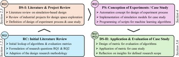
For investigation of the RQs, the Design Research Methodology (DRM) (Reference Blessing and ChakrabartiBlessing & Chakrabarti, 2009) was adapted and detailed. Based on a structured literature review, the research scope was defined according to the DRM Research Clarification stage (RC), resulting in the identified research gap. For the DRM Descriptive Study I stage (DS-I), typical design processes from literature and product optimisation projects were reviewed. This resulted in a generic description of a simulation-based optimisation approach for SE adapted from the DoE approach. Furthermore, a real-world case study was derived for evaluation. In the DRM Prescriptive Study stage (PS) an automation concept was designed and implementation of required simulation models as well as algorithms were performed. The DRM Descriptive Study II stage (DS-II) consists of design and application of a metric to assess the performance of ML algorithms and practical application in the specified case study. Figure 1 depicts an overview of the research design as well as sections of this paper addressing the DRM stages.
Research approach with allocated contribution to RQs and paper sections

2. Fundamentals
2.1. Basic terms
To identify related work and to clarify understanding of common terms, this section defines basic terms used in the paper. SE is a transdisciplinary and integrating approach for realisation, operation and decommissioning of technical systems by utilisation of system principles and concepts as well as scientific, technological and management methods (Reference Sillitto, Martin, McKinney, Griego, Dori and KrobSillitto et al., 2019; Reference Walden, Shortell, Roedler, Delicado, Mornas and Yew-SengWalden et al., 2023). In context of this paper, DSE in early stages of SE is investigated, specifically the system design before domain-specific development. DSE refers to the systematic investigation of possible design configurations (Reference Neubauer, Beichler and HaubeltNeubauer et al., 2020; Reference Pahl, Beitz, Feldhusen and GrotePahl et al., 2007) to identify solutions that satisfy defined design goals such as performance objectives or constraints. Each point in the design space represents a unique combination of design variables, e.g. geometry, material or technical or control parameters. In SBD the evaluation of design configurations is supported through digital simulations. Mostly, the goal is to understand trade-offs between conflicting objectives and to reveal relationships among design variables. By utilising SBDSE , simulation models are applied to balance exploration, exploitation and the refinement of promising areas in the design space. In most engineering applications, the investigation of trade-offs can be defined as MOO problem. MOO seeks a set of Pareto-optimal solutions where no objective can be improved without degrading another (Reference Collette and SiarryCollette & Siarry, 2004). The outcome of MOO is not a single best solution but the Pareto front, representing the set of optimal trade-offs in the objective space. This requires algorithms capable of addressing non-linear, non-convex and hyperdimensional problems. Due to the computational costs of complex simulations, SBDSE increasingly relies on learning-based strategies. In addition to classical methods, as Bayesian Optimisation or Particle Swarm Optimisation, ML approaches are alternatives that can predict desirable system qualities and guide evaluations efficiently, leading to data-driven design techniques. While RL and AL are established ML paradigms, the classification of EA as ML or classical statistical methods remains debated. Therefore, classification of EA as ML or as classical methods is based on preference. Consistent with recent research (Reference Telikani, Tahmassebi, Banzhaf and GandomiTelikani et al., 2021, Figure 1), this paper considers EA part of ML when applied for MOO.
2.2. Machine learning algorithms
Recent advances in ML offer new ways to accelerate SBDSE and MOO, using data-driven and adaptive search strategies. Three major algorithmic paradigms have proven particularly relevant in this context: EA (Reference Russell, Norvig and IntelligenceRussel & Norvig, 1995, pp. 79-80), RL (Reference Sutton and BartoSutton & Barto, 1998) and AL (Reference Granacher and MaréchalGranacher & Maréchal, 2022; Reference Jablonka, Jothiappan, Wang, Smit and YooJablonka et al., 2021). Each represents a distinct way of balancing information acquisition, search efficiency and optimisation performance in the pursuit of optimal design solutions. While more information can be found in the cited literature, they should be briefly introduced as follows.
EA are optimisation methods inspired by natural evolution and operating on populations of candidate design solutions. Populations evolve over generations through selection, crossover and mutation while candidates are evaluated using simulations as basis for fitness-based selection (Reference DebDeb, 2001). EA excel at MOO by exploring multiple regions of the design space simultaneously and approximating the Pareto front. Their robustness to non-linearity and noise makes them a standard choice in engineering design. However, numerous simulations make them computationally demanding, if each evaluation involves complex physics-based models. The following key terms apply if using EA for SBDSE applications:
-
• Population: Set of candidate designs being evolved in a specific iteration
-
• Fitness Function: Simulation-based measure to assess design quality
-
• Mutation/Crossover: Variation operators to introduce diversity for the next iteration
-
• Selection: Process of choosing high-performing candidates, e.g. for mutation/crossover
RL is an agent-based, sequential learning framework in which an agent interacts with an environment to learn a policy maximising long-term reward. In SBDSE, the agent adjusts design parameters (actions) based on simulation feedback (rewards) gained by the environment (simulation model) to learn strategies improving performance (Reference Sutton and BartoSutton & Barto, 1998). RL focuses on policy learning to develop a decision function that maps states to actions. RL methods are powerful in dynamic or adaptive design problems, where decisions unfold over multiple steps. Nevertheless, RL typically requires extensive simulation interactions and effectiveness depends on the reward design and exploration strategy (Reference Russell, Norvig and IntelligenceRussel & Norvig, 1995). Following key terms are relevant to discuss RL for SBDSE applications:
-
• Agent/Environment: Learner (Agent) and the simulation (Environment) providing feedback
-
• Action/State: Chosen design configuration (Action) and resulting product properties (State)
-
• Reward: Performance measure calculated based on simulation output/state
-
• Policy: Mapping from specific states to preferable actions
AL is a supervised learning approach reducing the number of simulations by strategically selecting the most informative design points. In SBDSE, it can be applied with predictors (e.g. Gaussian Processes or Neural Network Estimators) that approximate the qualities of design configurations (Reference Granacher and MaréchalGranacher & Maréchal, 2022; Reference Jablonka, Jothiappan, Wang, Smit and YooJablonka et al., 2021). The algorithm iteratively identifies areas of high model uncertainty and queries simulations to refine the predictors. Selective sampling of design configurations with the highest entropy (uncertainty in quality predictions) enables efficient learning and Pareto front identification with minimal simulation cost (Reference Bleisinger, Keil and EignerBleisinger et al., 2024). Following key terms are defined:
-
• Query Strategy: Rule for selecting new simulation points for sampling
-
• Scoring Function: Expression to calculate score (design quality) by simulation output
-
• Predictor: Entity predicting scores of design configurations without simulation runs
-
• Oracle: Source providing ground, which is the simulation in case of SBDSE
-
• Pool: The set of possible design configurations representing the whole design space
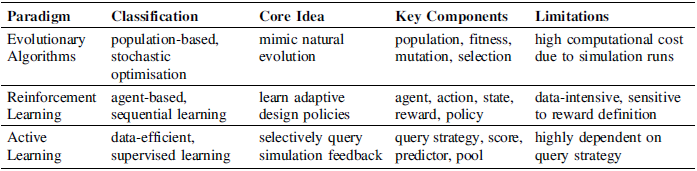
Table 1 summarises relevant key facts to compare differences between the three ML paradigms for DSE:
Comparison of different ML paradigms for SBDSE applications

3. Related work
3.1. State of the art for design exploration
SBDSE refers to the systematic search for Pareto-optimal solutions in high-dimensional design spaces where evaluation relies on simulations. Across engineering disciplines, including aerospace, mechanical engineering and materials science, simulation costs, e.g. for Computational Fluid Dynamics, Finite Element Analysis or multi-physics systems, is still a bottleneck (Reference Serani, Scholcz and VanziSerani et al., 2024). Classical approaches such as Grid Search or Monte-Carlo sampling require large numbers of evaluations, which become impractical when a single simulation takes minutes or hours on high-performance computers (Reference Lim, Jin, Ong and SendhoffLim et al., 2009). To overcome these limitations, recent research focuses on ML, particularly on surrogate or metamodel-based approaches that approximate costly simulations (Reference Bertoni, Hallstedt, Dasari and AnderssonBertoni et al., 2020; Reference García García, García Ródenas and Codina SanchoGarcía et al., 2020). Gaussian Processes, Random Forest regressors and various neural network applications, including Physics-Informed Neural Networks (Reference Raissi, Perdikaris and KarniadakisRaissi et al., 2019) and Graph Neural Networks are adopted as surrogate models with high accuracy and reduced computational costs (Reference Zhi, Wu, Qi, Zhu, Wu and WuZhi et al., 2023). Bayesian Optimisation leverages these surrogates by selecting new simulation points based on acquisition functions that balance exploration and exploitation (Reference CandelieriCandelieri, 2021). Beyond classical regression-based surrogates, generative models are increasingly applied. Variational Autoencoders and Generative Adversarial Networks provide low-dimensional latent representations of complex design spaces, enabling structured sampling and efficient optimisation (Reference Wang, Chan, Ahmed, Liu, Zhu and ChenWang et al., 2020; Reference Balmer, Kuhn, Bischof, Salamanca, Kaufmann, Perez-Cruz and KrausBalmer et al., 2024). For parametric simulations driven by partial differential equations, operator learning frameworks such as DeepONets and Fourier Neural Operators learn mappings between input parameters and full simulation fields (Reference Li, Huang, Liu and AnandkumarLi et al., 2023; Reference Romero, Rodríguez-Llorente, Magariños Rodríguez, Morant Navascués, Khvatkin Petrovsky, Lorenzo Ortega and Gómez-Espinosa MartínRomero et al., 2025). These models can evaluate faster than traditional numerical solvers, enabling near real-time DSE and interactive design workflows. Additional research focuses on more complex algorithmic architectures combining surrogates with physical models or utilising hybrid EA-RL approaches (Reference García García, García Ródenas and Codina SanchoGarcía et al, 2020; Reference KnowlesKnowles, 2006) as well as hybrid approaches coupling physical simulation, domain knowledge and ML. Recent research even combines SBDSE with uncertainty quantification, enabling surrogates to predict outputs as well as assess epistemic and aleatoric uncertainties for safety-sensitive engineering contexts. Techniques such as Sobol sensitivity indices or SHAP value analyses help designers interpret high-dimensional parameter interactions and understand trade-offs between competing objectives (Reference Weeratunge, Robe and HajizadehWeeratunge et al., 2025). Despite significant progress, surrogates struggle with extremely high-dimensional inputs or non-linear multi-physics interactions (Reference Lataniotis, Marelli and SudretLataniotis et al., 2020; Reference Grigo and KoutsourelakisGrigo & Koutsourelakis, 2017). Ensuring extrapolation, handling constraints correctly and combining data-driven models with physics-based solvers are open issues.
3.2. Metrics for algorithm comparison
To compare SBDSE for MOO applications from the ML paradigms of EA, RL and AL, existing metrics will be revised for evaluation of the investigated algorithms. Quantitative metrics measure different aspects in identifying the Pareto front, such as convergence to the true front, diversity of solutions and uniformity of coverage. They can be grouped into unary indicators and binary indicators . While binary indicators compare a solution set to a reference or benchmark set (e.g. the known Pareto front), unary indicators assess the quality of the algorithms without requiring a whole benchmark set. Unary indicators are useful in DSE because they allow the algorithm’s solution set to be evaluated on how well it covers and approximates the Pareto front, without the need to know the true Pareto front beforehand.
Hypervolume (HV): Captures both, convergence and diversity in a single measure and quantifies the hyperdimensional volume in the objective space that is dominated by a non-dominated solution set and bounded by a reference point. A larger hypervolume indicates better convergence to the Pareto front and broader coverage of the design space, making it a widely used metric in MOO (Reference Zitzler, Thiele, Laumanns, Fonseca and Da FonsecaZitzler et al., 2003).
Generational Distance (GD): Measures convergence of an approximated Pareto front to a reference front and calculates the average Euclidean distance between each solution in the set and its nearest point on the reference front. Smaller GD values indicate that the solutions are closer to the true Pareto front, reflecting better convergence. Requires the known Pareto front as reference (Reference Van VeldhuizenVan Veldhuizen, 1999).
Spacing (S): Evaluates the uniformity of solutions along an approximated Pareto front and calculates the standard deviation of the distances between consecutive solutions in the objective space. Smaller S values indicate a more uniform distribution of the solution set along the Pareto front (Reference SchottSchott, 1995).
Diversity Measure (Δ): Evaluates how well a solution set spans the range of the Pareto front and assesses both, the uniformity of neighbouring solutions and the coverage of the extreme points. Higher diversity values indicate better representation of trade-offs between objectives across the front (Reference Deb, Pratap, Agarwal and MeyarivanDeb et al., 2002).
Additive Epsilon Indicator (ϵ+): Measures the minimum additive shift required for a solution set to dominate all points of a reference set component-wise. Smaller values indicate a closer approximation to the reference front and better overall performance (Reference Zitzler, Thiele, Laumanns, Fonseca and Da FonsecaZitzler et al., 2003).
Multiplicative Epsilon Indicator (ϵ×): Measures the minimum multiplicative factor required for a solution set to dominate all points of a reference set (assuming positive objective values). Smaller values indicate a closer match to the reference front and better overall performance (Reference Zitzler, Thiele, Laumanns, Fonseca and Da FonsecaZitzler et al., 2003).
Binary indicators are useful as they provide a clear numerical comparison between the algorithm’s output and the optimal or best-known solutions if a pre-defined or the true Pareto front is known. HV stands out, combining convergence and diversity into a single measure. GD, in contrast, focuses purely on convergence, showing how close the solutions are to the true Pareto front but not addressing their spread. S and Δ complement this by quantifying the uniformity and coverage of the solutions, ensuring that trade-offs across objectives are well represented rather than clustered in certain regions of the objective space. The ϵ+ and ϵ× indicators provide a direct comparison against a reference front, offering a simple numerical assessment of how much the solutions would need to shift to dominate the benchmark. In SBDSE, using a combination of these metrics is valuable because it allows assessing not only how close the solutions are to the optimum, but also how well they cover the design space, thus giving a complete picture of algorithm performance in approximating the Pareto front.
4. Case study
4.1. Problem statement
In accordance with RQ1 and RQ2 from section 1.1, the problem statement in the case study can be briefly summarised as the task to automate DSE with an adapted DoE approach. Since the object under investigation is the ML-automated Pareto front identification, a real-world case study should be considered as exemplary DoE workflow to be automated. For reasons of publication (data availability) the vehicle to be optimised depicts a classical car with internal combustion engine, but the concepts are transferable to any kind of vehicle design. The case study is focused on DSE for vehicle conception within the development process of an automotive OEM. To predict and generate a data source for the ML algorithms, a simulation model is defined, which represents the transformation
 of the design space
 to the objective space
 , where
 is a design configuration and
 is the objective vector Equation (1):

In the mapping from design configurations to objective vectors,
 is the tyres rolling radius,
 is the final drive ratio and
 to
to
 are the ratios of gears 3 to 5. The design configuration is mapped to
 as total fuel consumption in the New European Driving Cycle (NEDC) from a roller test stand and
 to
to
 are the elasticity values for acceleration from 80 to 120 km/h. Since the mapping
 is non-linear it is evaluated by using simulations with a longitudinal vehicle model. The design goals are fuel efficiency and vehicle performance, reflected by reducing
 as well as
 ,
,
 and
and
 simultaneously. To assess the design configuration quality
 and parametrise the algorithms (reward/score/fitness), the following statement is derived in multiple steps by assumptions for importance of design characteristics Equation (2):

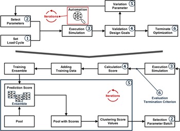
The SBDSE approach is an adapted DoE process which is derived from elicitation at an automotive OEM and the manual process consists of the following steps depicted in Figure 2 (top).
-
• Step 1: Definition of relevant load cycle, e.g. the NEDC
-
• Step 2: Selection of a specific design configuration
 (design parameters)
 -
• Step 3: Evaluation (simulation) run to derive
as objective vector -
• Step 4: Inspection of
and decision on meeting or failing design goals -
• Step 5: Adjustments of components of the design configuration variable
for next iteration -
• Step 6: Termination of optimisation process, if required design goals are met


Simplified view on DoE approach (top) and exemplary automation approach on the example of AL (bottom) as extract from previous work (Reference Bleisinger and EignerBleisinger & Eigner, 2025)

In the case study the load cycles are stable through the iterations after the initial setup. While the NEDC roller stand measurement data is the main load cycle to calculate fuel consumption, a full throttle scenario at maximum acceleration is the second load cycle to calculate the elasticity values. The objective of the ML algorithms is the automation of SBDSE iterations and finding the Pareto front. Figure 2 (bottom) shows exemplarily how this can be achieved by the AL approach. Further details and explanations on constraints of the design space in the MOO of the case study as well as pseudocode for the AL implementation can be found in previous publications of the authors (Reference Bleisinger, Keil and EignerBleisinger et al., 2024).
4.2. Automation concept
To realise the automation according to Figure 2 (top), algorithms from EA, RL and AL according to Table 1 are utilised. To demonstrate the diversity and potential of learning-based optimisation, four representative algorithms were examined: Non-Dominated Sorting Genetic Algorithm II (NSGA-II) (Reference Chaturvedi, Rajasekar and NatarajanChaturvedi et al., 2020; Reference Deb, Pratap, Agarwal and MeyarivanDeb et al., 2002; Reference Rahimi, Gandomi, Nikoo and ChenRahimi et al., 2023), Soft Actor-Critic (SAC) (Reference Haarnoja, Zhou, Abbeel and LevineHaarnoja et al., 2018; Reference Kathirgamanathan, Mangina and FinnKathirgamanathan et al., 2021), Asynchronous Advantage Actor-Critic (A3C) (Reference Mnih, Badia, Mirza, Graves, Lillicrap, Harley, Silver and KavukcuogluMnih et al., 2016; Reference Bleisinger, Keil, Stuppy and MalekBleisinger et al., 2023) and Greedy Active Learning (GAL) (Reference Bleisinger, Keil and EignerBleisinger et al., 2024). To ensure comparability, the algorithms were implemented on the same case study according to the problem statement in section 4.1. Implementations were performed in the years 2022-2025 by the authors.
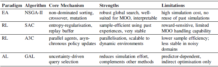
NSGA-II is a well-known algorithm for MOO which sorts candidate designs into different levels based on whether one design dominates another. To keep the population diverse and explore trade-offs, the algorithm uses a crowding distance. In SBDSE, NSGA-II is valued for its robustness and the fact that it directly produces a set of Pareto-optimal designs. However, it requires large numbers of simulation runs and does not learn from past experiences, which makes it computationally expensive. NSGA-II is often used as a benchmark to evaluate newer ML algorithms (Reference Chaturvedi, Rajasekar and NatarajanChaturvedi et al., 2020; Reference Deb, Pratap, Agarwal and MeyarivanDeb et al., 2002; Reference Rahimi, Gandomi, Nikoo and ChenRahimi et al., 2023). SAC is a RL method that learns through trial and error by interacting with an environment. It is an off-policy, model-free approach that adds an entropy term to encourage exploration. SAC learns two functions at the same time: an actor that defines how to act and a critic that evaluates the expected performance of those actions. The entropy ensures improving both, stability and learning efficiency. In SBDSE, SAC can be used to automatically adjust design parameters based on simulation results. It works well for problems with continuous and noisy variables, although the use in MOO often requires combining several objectives in scalar reward function (Reference Haarnoja, Zhou, Abbeel and LevineHaarnoja et al., 2018; Reference Kathirgamanathan, Mangina and FinnKathirgamanathan et al., 2021). The A3C algorithm is an on-policy RL approach and runs multiple agents in parallel, each exploring the environment and updating a shared model asynchronously. An advantage function helps the algorithm learn faster by estimating how much better a specific action is compared to the average action. In SBDSE, A3C is useful for large or dynamically changing design spaces, as parallelisation allows fast coverage and learning. However, unlike SAC, A3C cannot reuse past experiences, which reduces its sample efficiency. In theory, this makes it less suitable if simulation is very costly (Reference Mnih, Badia, Mirza, Graves, Lillicrap, Harley, Silver and KavukcuogluMnih et al., 2016). AL is a strategy that focuses on selecting the most informative data points to evaluate in the next simulation run. In SBDSE, it is combined with a predictive model which estimates performance outcomes across the design space. AL chooses new simulations in regions where the model is uncertain or improvement seems likely, reducing the total number of simulations to cover important areas of the design space. It can be applied with simple query strategies or combined with algorithms like NSGA-II or RL methods to guide exploration towards promising regions, improving data efficiency and reducing computational effort (Reference Granacher and MaréchalGranacher & Maréchal, 2022). For evaluation in this paper, implementation with a greedy query strategy is used, leading to the GAL approach (Reference Bleisinger, Keil and EignerBleisinger et al., 2024). Each of these algorithms offers unique benefits for SBDSE. NSGA-II provides a reliable baseline, while SAC and A3C introduce adaptive, policy-based learning. AL complements both by reducing simulation costs and focusing effort on relevant regions of the design space. Table 2 summarises a comprehensive view.
Overview of selected algorithms from different machine learning paradigms

5. Evaluation results
5.1. Experimental setup
As stated by Equation 1, the evaluation of the algorithms is based on a MOO problem from automotive design in SE. The aim is to optimise competing system properties of a vehicle while respecting design constraints. The MOO involves four objectives to be minimised and five design parameters, whereby a strict monotonicity constraint is imposed on the gear ratios (
 ). Simulation is performed using a MATLAB/Simulink model for the longitudinal vehicle model, calibrated with experimental data from roller test stands and executing the NEDC as well as a full-throttle acceleration scenario. The model functions as a black box connected to the optimisation algorithms, enabling the mapping of design configurations to objective vectors by the function
 in Equation 1. GAL, A3C, SAC and NSGA-II were adapted to respect input bounds, with NSGA-II applying clipping during mutation and RL methods normalising actions via a
 -transformation. For GAL, A3C and SAC, a common scoring/reward function derived from Equation 2 evaluates candidate solutions based on contribution to approximating the Pareto front. NSGA-II employs non-dominated sorting with crowding distance, ensuring comparability with the other methods. Hyperparameter optimisation is conducted using Optuna with a Tree-structured Parzen Estimator, avoiding bias from suboptimal settings. Each algorithm is allocated a fixed evaluation budget of 100 simulations per run, performed over 10 randomly selected seeds. Algorithm performance is evaluated by solution quality and computational effort. Hypervolume is used as the primary metric for solution quality, complemented by a measure of solution spread along the objective space (see section 3.2). Computational effort is measured by the number of simulation calls. Robustness is assessed through repeated runs, reporting mean, standard deviation and variance for each method. Statistical significance of differences between algorithms is evaluated using the Friedman test, which does not require assumptions about the underlying distributions. In cases where significant differences are detected, a Nemenyi post-hoc test is applied to identify pairwise differences. All experimental conditions were reproducible, with the same hardware and software environment.
5.2. Results
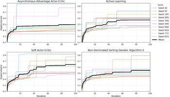
Figure 3 shows the evolution of hypervolume over iterations for all algorithms. Overall, hypervolume increases monotonically, rising steeply at first, reaching initial plateaus and then improving in stepwise jumps that decrease in frequency and magnitude toward the end. A3C exhibits high variability between seeds, with some runs reaching high hypervolume (>0.75) while others remain low (∼0.35), resulting in a mean of 0.49. SAC achieves the highest mean hypervolume of 0.63, with two seeds reaching around 0.80. GAL reaches a mean of 0.57 with moderate variability and NSGA-II shows initial rapid gains followed by mid-level plateaus, ending at 0.55. Friedman testing indicates a significant effect of algorithm on hypervolume (p=0.048), with post-hoc Nemenyi analysis showing SAC significantly outperforms A3C. No significant differences were found for diversity (p=0.717). Examination of Pareto fronts reveals that high hypervolume solutions are represented by few points, while lower hypervolume fronts contain many solutions. This indicates that differences in hypervolume are primarily due to reach toward extreme points rather than front coverage. Observed patterns may be due to limited exploration, potential global optima or simplifications in the simulation model. The experiments ensure comparison across algorithms, with evaluations over ten seeds and consistent reference points. Some solutions violated manual bounds, affecting hypervolume without altering Pareto front behaviour. A3C results are additionally subject to CPU-induced randomness. SAC achieves the highest hypervolume with long runtimes. NSGA-II reaches highest diversity and A3C provides the most stable but low performance. Results are influenced by simulation budgets, offering practical guidance rather than absolute rankings.
Results for hypervolume of runs on different starting seeds A3C, SAC, GAL, NSGA-II

6. Conclusion & limitations
In this contribution a comparison of the ML paradigms EA, RL, AL was performed based on algorithm implementation and application of performance indicators in a case study for SBDSE. Based on the results of a literature review, it is concluded that the hypervolume is the only existing unary indicator for DSE. Thus, it can be considered the only well-known unary indicator to assess and compare different ML algorithms in SBDSE. It can be complemented by binary indicators for coverage or spread along Pareto fronts such as Generational Distance, Spacing or Diversity Measure (see section 3.2). Main limitations in this conclusion are the accessibility of publications on performance indicators and the search strategy based on keywords for the research design defined in Figure 1. It should be noted, that the hypervolume indicator is sensitive to selection of the reference point. Still, it remains a suitable performance indicator in Pareto front identification of different algorithms since the concrete reference point for hypervolume calculation is considered a minor issue for qualitative comparison of algorithms. Regarding RQ2, the main insight is that EA, which were originally developed for DSE in MOO settings, can be outperformed by more modern ML approaches. Although this insight cannot be generalised, it was shown by the case study, that SAC might perform well in SBDSE tasks. Multiple limitations need to be considered regarding this assumption. The most significant limitation is the limited case study which might bias algorithm performance due to the constraints and shape of the design space - since not all algorithms can natively handle constraints. Additionally, the identification of the Pareto front with RL and AL approaches is dependent on the reward/scoring function as well as the simulation budget. Thus, reward/scoring functions (see Equation 2) equally balancing weights of the competing design goals in the case study were selected. This limitation was investigated in previous work of the authors of this contribution and is considered highly relevant for future work. Furthermore, the performance of all algorithms is sensitive to tuning of hyperparameters. Although a fair and comparable method for hyperparameter tuning was adapted, it remains future work to investigate the concrete sensitivity of algorithm performance to a potential suboptimal selection of neural network hyperparameters.

 Open access

