


1. Introduction
Variations in bed properties that affect basal sliding, such as the distribution of deformable sediment versus hard bedrock, significantly impact the dynamics of large ice masses. To account for the impact of these bed heterogeneities on ice flow, models of ice-sheet and glacier evolution require appropriate boundary conditions at the ice-bedrock interface. As the glacier bed remains challenging to observe, these basal boundary conditions can only very rarely be directly specified (e.g. Cohen and others, Reference Cohen, Hooke, Iverson and Kohler2000; Iverson and others, Reference Iverson2007; Vincent and Moreau, Reference Vincent and Moreau2016). Instead, inferring basal properties such as basal sliding can be achieved by assimilating remotely sensed or direct measurements of surface flow with an ice-flow model in an inverse modelling framework. Practically, observed surface flow velocities are commonly used to constrain basal sliding. The increase in both spatial and temporal resolution in datasets has driven and will continue to drive developments that deliver more accurate projections of ice flow in a changing climate.
Many previous studies have deduced basal stresses or sliding coefficients under modern ice sheets and glaciers, pioneered by MacAyeal (Reference MacAyeal1992, Reference MacAyeal1993) and adapted, for instance, by Vieli and Payne Reference Vieli and Payne(2003) and Joughin and others (Reference Joughin, MacAyeal and Tulaczyk2004). These early studies were applied to limited regional-scale applications using the shallow shelf approximation equations appropriate for stretching flow and using control, or adjoint, methods to invert for basal properties. Recent studies using a similar approach have been applied, for example, to the Pine Island/Thwaites Glacier areas and to continental Antarctica (Vieli and Payne, Reference Vieli and Payne2003; Morlighem and others, Reference Morlighem, Seroussi, Larour and Rignot2013). Other examples are Price and others Reference Price, Payne, Howat and Smith(2011), who applied a simpler inversion method to Greenland, and Le Brocq and others Reference Le Brocq, Payne, Siegert and Alley(2009), who linked a similar method with a basal hydrology model for West Antarctica. More recently, the initMIP-Greenland and initMIP-Antarctica intercomparison studies (Goelzer and others, Reference Goelzer2018a; Seroussi and others, Reference Seroussi2019) showed how data assimilation improves ice-sheet model initialisation by comparing various methods to incorporate observational data. All these studies are based on fitting modelled ice velocities to observed surface or balance velocities, with ice surface elevations prescribed based on digital elevation models. A similar approach but fitting ice thickness instead of ice velocity has been used as well (e.g. Pollard and DeConto, Reference Pollard and DeConto2012; Le clec’h and others, Reference Le clec’h, Quiquet, Charbit, Dumas, Kageyama and Ritz2019).
For alpine glaciers, significant research is focused on estimating the ice thickness and surface mass balance (SMB) to project volume estimates into the future (Farinotti and others, Reference Farinotti, Huss, Bauder, Funk and Truffer2009, Reference Farinotti2017, Reference Farinotti2021; Zekollari and others, Reference Zekollari, Huss and Farinotti2019). In these studies, basal sliding is usually accounted for by assuming that a fixed fraction of the surface velocity is attributed to sliding, and the inversion is typically based on a combination of physics-based and empirical relations (Zekollari and others, Reference Zekollari, Huss, Farinotti and Lhermitte2022). In some cases, 1-D flowline models are employed to reconstruct the bedrock topography using Bayesian inference (Werder and others, Reference Werder, Huss, Paul, Dehecq and Farinotti2020), with the glacier sliding assumed to be constant. Notable exceptions that present inversions for basal sliding include Gilbert and others Reference Gilbert, Sinisalo, Gurung, Fujita, Maharjan, Sherpa and Fukuda(2020) and Schäfer and others Reference Schäfer, Möller, Zwinger and Moore(2015), where an adjoint-based method is used to invert spatially variable basal friction from observed surface velocities using a 3-D Stokes model, but without considering geometry evolution, and Jouvet Reference Jouvet(2023), where the distribution of the sliding parameter is reconstructed using a deep learning ice-flow emulator.
Most inversions of basal properties in glaciology make use of the fact that glaciers and ice sheets behave as a Stokes flow, i.e. that the flow velocity has no history dependence. This means that, in theory, for a given ice geometry and boundary conditions the ice-flow velocity is fully determined; conversely, given observations of ice geometry and velocity, the boundary conditions can be inverted. Notably, neither the SMB nor the evolution of the ice geometry is needed for this type of inversion, which is called snapshot inversion (Morlighem and Goldberg, Reference Morlighem, Goldberg, Ismail-Zadeh, Castelli, Jones and Sanchez2023). Unlike the velocity, the evolution of the ice geometry, driven by ice flow, mass balance and mass conservation, is history-dependent. Consequently, if an inversion aims to use the often available observations of geometry evolution, it will need to be a so-called time-dependent inversion (Morlighem and Goldberg, Reference Morlighem, Goldberg, Ismail-Zadeh, Castelli, Jones and Sanchez2023).
In general, it is desirable to use as much available data as possible to better constrain the quantity being inverted. For instance, it has been observed that forward model runs using basal boundary conditions from snapshot inversions frequently exhibit significant initial changes in geometry, such as unrealistically high rates of surface elevation change (e.g. Joughin and others, Reference Joughin, Tulaczyk, Bamber, Blankenship, Holt, Scambos and Vaughan2009; Goldberg and Heimbach, Reference Goldberg and Heimbach2013). Using the additional information of observed geometry changes in time-dependent inversions may address such issues (Morlighem and Goldberg, Reference Morlighem, Goldberg, Ismail-Zadeh, Castelli, Jones and Sanchez2023).
The adjoint state method (Giles and Pierce, Reference Giles and Pierce2000) is one of the few practical ways to perform high-resolution inversions and is regularly applied in glaciology both for snapshot and time-dependent inversions (Morlighem and Goldberg, Reference Morlighem, Goldberg, Ismail-Zadeh, Castelli, Jones and Sanchez2023). The main advantage of this method is that the cost of evaluating the gradient of the objective function, i.e. the function which needs to be minimised in the inversion, is only one forward solve and one linear adjoint solve. The main disadvantages are posed by the complex derivation of the adjoint state equations and the risk of the inversion being trapped in a local minimum. Adjoint-based inversions, used to optimise parameters such as ice-flow properties, require computing the gradient of an objective function, which is often complex and high-dimensional. Deriving this gradient manually is both time-consuming and error-prone. Therefore, automatic differentiation (AD), which can differentiate computer code directly, has become a preferred approach to accurately calculate such gradients (e.g. Heimbach and others, Reference Heimbach, Hill, Giering, Sloot, Hoekstra, Tan and Dongarra2002; Goldberg and Heimbach, Reference Goldberg and Heimbach2013; Morlighem and Goldberg, Reference Morlighem, Goldberg, Ismail-Zadeh, Castelli, Jones and Sanchez2023).
As stated above, time-dependent inversions are a way to include more data in inversions with the potential to achieve higher fidelity. Compared to snapshot inversions, taking time into account adds an additional dimension, resulting in a more demanding approach in terms of both implementation, e.g. using the adjoint state method, and computational resources. These kind of inversions were pioneered in glaciology over the last two decades (Morlighem and Goldberg, Reference Morlighem, Goldberg, Ismail-Zadeh, Castelli, Jones and Sanchez2023). Early time-dependent inversions used 1-D flowline models to examine the history of accumulation of ice sheets, via internal layer information (Waddington and others, Reference Waddington, Neumann, Koutnik, Marshall and Morse2007; Koutnik and others, Reference Koutnik2016), or used time-dependent geometry evolution data for ice thickness estimations of mountain glaciers (Michel and others, Reference Michel, Picasso, Farinotti, Bauder, Funk and Blatter2013). Goldberg and Heimbach (Reference Goldberg and Heimbach2013), Larour and others (Reference Larour2014) and Goldberg and others Reference Goldberg, Heimbach, Joughin and Smith(2015) pioneered time-dependent inversions on ice-sheet catchment scale using depth-integrated, higher-order ice-flow models. They employed above-mentioned adjoint state method combined with AD in order to construct the needed gradients to optimise the time-dependent cost function. The combination of these two methods made both the code development and computation tractable. Since then a number of studies have applied variations of this type of approach (e.g. Koziol and others, Reference Koziol, Todd, Goldberg and Maddison2021; Morlighem and others, Reference Morlighem, Goldberg, Dias Dos Santos, Lee and Sagebaum2021; Choi and others, Reference Choi, Seroussi, Morlighem, Schlegel and Gardner2023). More recently, methods based on statistical methods have been employed for time-dependent inversions, such as Kalman filters (Gillet-Chaulet, Reference Gillet-Chaulet2020) or Bayesian approaches (Brinkerhoff and others, Reference Brinkerhoff2024). While above research shows that time-dependent inversions are becoming more common in glaciology, unlike snapshot inversions, they are not routinely employed yet and are still in development in the major ice-sheet models the community uses (Morlighem and Goldberg, Reference Morlighem, Goldberg, Ismail-Zadeh, Castelli, Jones and Sanchez2023).
Recent advances in computer hardware, programming languages and computational tools have led to significant progress in scientific computing in glaciology. Graphics processing units (GPUs) offer orders of magnitude speed-up over traditional CPU-based computations (Sandip and others, Reference Sandip, Räss and Morlighem2024) and have been utilised in glaciology since the early days of general-purpose GPU computing (Bræ dstrup and others, Reference Brædstrup, Damsgaard and Egholm2014). Today, GPUs have been used for large-scale, 3-D, Stokes models (Räss and others, Reference Räss, Licul, Herman, Podladchikov and Suckale2020) and climate inversions based on palaeo-glacier extents (Visnjevic and others, Reference Visnjevic, Herman and Podladchikov2018). However, GPUs remain underused in glaciology, particularly compared to their adoption in fields such as climate modelling. To date, none of the widely used numerical ice-sheet models incorporate GPU capabilities, highlighting the need for further development in this area.
Recent developments, largely driven by artificial intelligence research, have enhanced tools and programming languages that support AD of CPU and GPU codes, making these approaches more accessible and efficient. Frameworks such as dolfin-adjoint enable adjoint code generation on CPUs (Mitusch and others, Reference Mitusch, Funke and Dokken2019), while GPU-enabled computational frameworks like TensorFlow have enabled deep learning-based surrogates (Brinkerhoff and others, Reference Brinkerhoff, Aschwanden and Fahnestock2021; Jouvet and Cordonnier, Reference Jouvet and Cordonnier2023; Jouvet, Reference Jouvet2023) and physics-informed neural networks for ice-flow simulations and inversions (Jouvet and Cordonnier, Reference Jouvet and Cordonnier2023).
However, these frameworks often have limitations in terms of flexibility and performance. Newer programming languages, such as Julia (Bezanson and others, Reference Bezanson, Edelman, Karpinski and Shah2017), overcome many of these issues by combining ease of use with state-of-the-art performance across multiple computing platforms, including GPUs (Räss and others, Reference Räss, Utkin, Duretz, Omlin and Podladchikov2022). Additionally, Julia supports AD for nearly the entire language, further enhancing its utility in scientific computing. For example, Bolibar and others Reference Bolibar, Sapienza, Maussion, Lguensat, Wouters and Pérez(2023) utilise Julia to develop an approach that combines physics-based and machine learning-based simulations to invert for ice-flow parameters of mountain glaciers.
The main aim of this study is to provide an automated and computationally efficient AD and GPU-based procedure for time-dependent inversions of the spatial distribution of the basal sliding coefficient. This inversion procedure is then assessed by (i) studying the differences between snapshot and time-dependent inversions; (ii) verifying our approach on a synthetic test case; and (iii) applying it to the Aletsch glacier in the Swiss Alps. First, we present the methods detailing our approach to inverse modelling using the adjoint state method. Next, we outline the numerical implementation, demonstrating how we leverage AD on GPUs using Julia. Subsequently, we describe the two different model configurations that we investigate: the snapshot and time-dependent cases, which are applied to both a synthetic example and Aletsch glacier. Finally, we present the results, discuss their implications and provide an outlook on how to extend this work.
2. Methods
By using inverse modelling, we seek a better understanding of the complex motion of glaciers partially sliding over the bed. To achieve this goal, we solve an optimisation problem to estimate the hidden basal state of glaciers by leveraging observations of ice surface velocities from remote sensing or sparse direct measurements. Additionally, as we continue to develop the method, we incorporate ice surface elevation changes recorded in digital elevation models taken at different moments in time.
In this study, we consider two inversion approaches: snapshot and time-dependent. In snapshot inversion, the geometry of the glacier is assumed to be known from observations at a given time, and only the instantaneous velocity distribution at that point in time is used to reconstruct the sliding parameter. Snapshot is a commonly used inversion approach since it has the advantage of not requiring any information on the SMB. However, when using the results of the snapshot inversion to integrate the ice-flow model forward in time, the predicted velocities and geometry changes might exhibit unrealistic variations due to the lack of temporal information (Joughin and others, Reference Joughin, Tulaczyk, Bamber, Blankenship, Holt, Scambos and Vaughan2009; Goldberg and Heimbach, Reference Goldberg and Heimbach2013), discrepancies between different data products and insufficient spatial coverage of the observations. These issues can be partially addressed by the time-dependent inversion, which takes into account both the velocity and geometry change observations and assimilates them in a transient ice-flow model. While producing potentially more robust reconstructions of the sliding parameter with respect to the observations, this inversion approach is more computationally demanding, especially for large-scale inversions. Our framework has the potential to enable inverse modelling on larger problems by leveraging massively parallel GPU computing both for running the forward model and for the computation of the gradients.
In this study, we are using the depth-averaged shallow ice approximation (SIA) as the forward model with the assumption that the horizontal scale of the ice extent is much larger than the vertical extent (Cuffey and Paterson, Reference Cuffey and Paterson2006). The SIA provides a simplification of the Stokes equations at the expense of less accurate results near the margin and ice divide. Despite the limitations of SIA when modelling mountain valley glaciers or ice sheets (e.g. only 3 out of the 37 simulations included in ISMIP6 for both Greenland and Antarctica use SIA (Goelzer and others, Reference Goelzer2018b; Seroussi and others, Reference Seroussi2019)), the computational efficiency and simplicity of SIA represent an advantage for large-scale applications and long-term simulations. A decrease in computational cost renders the SIA model also attractive in providing an efficient way to initialise more complex ice-flow models for specific conditions or to fit observational data (Arthern and Gudmundsson, Reference Arthern and Gudmundsson2010). The SIA model is thus sufficient for the present work, the purpose of which lies mainly in exploring the inversion methods and their efficient numerical implementation.
In both snapshot and time-dependent inversion approaches, our goal is to determine the spatially varying sliding parameter  $A_{\mathrm{s}}$ that minimises the following objective functional:
 \begin{equation}
\mathcal{J}(A_{\mathrm{s}}) = {\mathcal{J}}_{\mathrm{obs}}(A_{\mathrm{s}}) + \gamma {\mathcal{J}}_{\mathrm{reg}}(A_{\mathrm{s}}).
\end{equation}
\begin{equation}
\mathcal{J}(A_{\mathrm{s}}) = {\mathcal{J}}_{\mathrm{obs}}(A_{\mathrm{s}}) + \gamma {\mathcal{J}}_{\mathrm{reg}}(A_{\mathrm{s}}).
\end{equation} Here,  ${\mathcal{J}}_{\mathrm{obs}}$ is the observational component of the total misfit, ${\mathcal{J}}_{\mathrm{reg}}$ is the Tikhonov regularisation component and γ is a tunable parameter designed to prevent overfitting.
In this study, we define  $\mathcal{J}_{\mathrm{reg}}$ as the norm of the gradient of $\log A\mathrm{s}$:
 \begin{equation}
{\mathcal{J}}_{\mathrm{reg}}(A_{\mathrm{s}}) = \frac{1}{2}\sum_i \left( \nabla \log A_{\mathrm{s}_i} \right)^2,
\end{equation}
\begin{equation}
{\mathcal{J}}_{\mathrm{reg}}(A_{\mathrm{s}}) = \frac{1}{2}\sum_i \left( \nabla \log A_{\mathrm{s}_i} \right)^2,
\end{equation} where i is the grid point index. With this choice of regularisation, larger values of γ result in a smoother distribution of  $A_{\mathrm{s}}$. It is important to note that the regularisation term involves the logarithm of $A_{\mathrm{s}}$. This approach is adopted because the inversion is performed in a logarithmic scale, allowing us to better capture the wide range of values while ensuring the positivity of $A_{\mathrm{s}}$.
2.1. Snapshot inversion
In the snapshot approach, we fix the surface elevation data from the observations and seek to find the sliding coefficient distribution that leads to modelled surface velocities matching observations. We define the observational part of the objective function as a spatially integrated difference between surface velocity magnitude obtained from the model and the observed surface velocity magnitude:
 \begin{equation}
\mathcal{J}^\mathrm{s}_{\mathrm{obs}}(A_{\mathrm{s}}) = \frac{\omega_V}{2}\sum_{i}\left(V_i(A_{\mathrm{s}}) - V_i^{\mathrm{obs}}\right)^2,
\end{equation}
\begin{equation}
\mathcal{J}^\mathrm{s}_{\mathrm{obs}}(A_{\mathrm{s}}) = \frac{\omega_V}{2}\sum_{i}\left(V_i(A_{\mathrm{s}}) - V_i^{\mathrm{obs}}\right)^2,
\end{equation} where  $V_i(A_{\mathrm{s}})$ is the surface velocity computed according to the forward model, $V_i^{\mathrm{obs}}$ denotes the observed surface velocity magnitude.
To normalise the first term, we use the parameter ωV as the inverse of the L 2-norm of the observed velocity field:
 \begin{equation}
\omega_V = \left[\sum_i\left(V^{\mathrm{obs}}_i\right)^2\right]^{-1}.
\end{equation}
\begin{equation}
\omega_V = \left[\sum_i\left(V^{\mathrm{obs}}_i\right)^2\right]^{-1}.
\end{equation}2.2. Time-dependent inversion
In the time-dependent approach, we seek to reconstruct the sliding coefficient  $A_{\mathrm{s}}$ distribution by fitting both the magnitude of the modelled surface velocity and the geometry of the ice over a defined time period. In this case, the observational part of the objective functional $\mathcal{J}^\mathrm{td}_{\mathrm{obs}}(A_{\mathrm{s}})$ measures the total spatially integrated differences between modelled and observed surface velocity and ice thickness with ωV and ωH as normalisation weights:
 \begin{equation}
\mathcal{J}^\mathrm{td}_{\mathrm{obs}}(A_{\mathrm{s}}) = \frac{\omega_V}{2}\sum_{i}\left(V_i(A_{\mathrm{s}}) - V_i^{\mathrm{obs}}\right)^2 + \frac{\omega_H}{2}\sum_{i}\left(H_i(A_{\mathrm{s}}) - H_i^{\mathrm{obs}}\right)^2,
\end{equation}
\begin{equation}
\mathcal{J}^\mathrm{td}_{\mathrm{obs}}(A_{\mathrm{s}}) = \frac{\omega_V}{2}\sum_{i}\left(V_i(A_{\mathrm{s}}) - V_i^{\mathrm{obs}}\right)^2 + \frac{\omega_H}{2}\sum_{i}\left(H_i(A_{\mathrm{s}}) - H_i^{\mathrm{obs}}\right)^2,
\end{equation} where  $H_i(A_{\mathrm{s}})$ is the modelled ice thickness corresponding to the parameter $A_{\mathrm{s}}$, and $H_i^{\mathrm{obs}}$ is the observed ice thickness. The modelled ice thickness H in (5) is defined at the same moment in time as the observed ice thickness $H^{\mathrm{obs}}$. We approximate the average annual velocity using the velocity distribution V at the end of the time integration period. Note that (5) does not include summation over time. In this study, we assimilate only one velocity and ice thickness dataset in the time-dependent inversion, and thus, we omit the summation.
We define the parameters ωV and ωH as the weighted inverse of the L 2-norm of the observed velocity and ice thickness fields, respectively:
 \begin{gather}
\omega_V = \omega^n_V \left[ \sum_i\left(V^{\mathrm{obs}}_i\right)^2\right]^{-1},
\end{gather}
\begin{gather}
\omega_V = \omega^n_V \left[ \sum_i\left(V^{\mathrm{obs}}_i\right)^2\right]^{-1},
\end{gather} \begin{gather}
\omega_H = \omega^n_H \left[ \sum_i\left(H^{\mathrm{obs}}_i\right)^2\right]^{-1},
\end{gather}
\begin{gather}
\omega_H = \omega^n_H \left[ \sum_i\left(H^{\mathrm{obs}}_i\right)^2\right]^{-1},
\end{gather} \begin{gather}
\sqrt{\left(\omega^n_V\right)^2 + \left(\omega^n_H\right)^2} = 1,
\end{gather}
\begin{gather}
\sqrt{\left(\omega^n_V\right)^2 + \left(\omega^n_H\right)^2} = 1,
\end{gather} where  $\omega^n_V$ and $\omega^n_H$ are normalised weights representing the relative influence of velocity and ice thickness, respectively.
2.3. Forward model
In this study, we use the isothermal SIA as the forward model both for the snapshot and time-dependent inversion approaches. According to the SIA, the surface velocity V is given by:
 \begin{equation}
V = \left(\rho g\right)^n \left[\frac{2}{n+1} A H^{n+1} + A_{\mathrm{s}} H^n \right] \left| \nabla S \right|^{n},
\end{equation}
\begin{equation}
V = \left(\rho g\right)^n \left[\frac{2}{n+1} A H^{n+1} + A_{\mathrm{s}} H^n \right] \left| \nabla S \right|^{n},
\end{equation} where  $S = B + H$ is the ice surface elevation, B is the bed elevation, ρ is the ice density, g is the gravitational acceleration, A is the ice-flow parameter, $A_{\mathrm{s}}$ is the sliding parameter and n is Glen’s flow law exponent (Glen, Reference Glen1958). The first term in brackets of (9) represents the flow due to ice deformation and the second term due to sliding following a Weertman-like sliding law (Fowler and Frank, 1997) where all constants are lumped into $A_{\mathrm{s}}$.
The constants of the ice-flow model are listed in Table 1. To account for the discrepancies introduced by using the simplified ice-flow description, we introduce the correction factor E to define the ice-flow parameter A:
 \begin{equation}
A = E A_0,
\end{equation}
\begin{equation}
A = E A_0,
\end{equation}Forward ice-flow model parameters
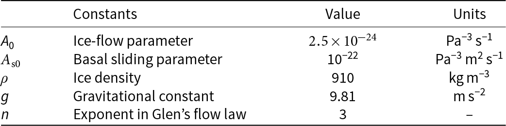
where A 0 is the reference value of the ice-flow parameter. We vary the value of E depending on the problem set-up but keep it constant in time and space, assuming that most of the variability in the results can be attributed to the local changes in sliding. We consider the ice to be temperate, and all temperature-dependent constants listed in Table 1 are computed at  $T=0^\circ\mathrm{C}$.
The evolution of the ice thickness H is described by the depth-averaged mass conservation equation:
 \begin{equation}
\frac{\partial H}{\partial t} = -\nabla \cdot \boldsymbol{q} + \dot{b} ,
\end{equation}
\begin{equation}
\frac{\partial H}{\partial t} = -\nabla \cdot \boldsymbol{q} + \dot{b} ,
\end{equation} where q is the horizontal ice flux and  $\dot{b}$ is the volumetric SMB rate, i.e. the rate of ice accumulation and ablation at a point. The horizontal ice flux q is defined as the vertically integrated velocity field:
 \begin{equation}
\boldsymbol{q} = \int_{B}^{S}\boldsymbol{V}(z)\,\mathrm{d}z.
\end{equation}
\begin{equation}
\boldsymbol{q} = \int_{B}^{S}\boldsymbol{V}(z)\,\mathrm{d}z.
\end{equation} We define the SMB  $\dot{b}$ as:
 \begin{equation}
\dot{b} = \min \left\{c (S - z_\mathrm{ELA}), ~\dot{b}_\mathrm{max} \right\} ,
\end{equation}
\begin{equation}
\dot{b} = \min \left\{c (S - z_\mathrm{ELA}), ~\dot{b}_\mathrm{max} \right\} ,
\end{equation} where c is the mass-balance rate gradient, S is the surface elevation,  $z_\mathrm{ELA}$ is the equilibrium line altitude and $\dot{b}_\mathrm{max}$ is the maximum ice accumulation rate (Meier, Reference Meier1962). This piecewise linear relation reflects the observation that the dependence of the mass balance on the elevation is usually stronger in the ablation area than in the accumulation area (Mayo, Reference Mayo1984).
Following the approach of Hindmarsh and Payne Reference Hindmarsh and Payne(1996), the ice-flow equation (11) can be regarded as a nonlinear diffusion-reaction equation with a nonlinear diffusion coefficient D and horizontal diffusion flux q:
 \begin{gather}
\boldsymbol{q} = -D ~ \nabla S ,
\end{gather}
\begin{gather}
\boldsymbol{q} = -D ~ \nabla S ,
\end{gather} \begin{gather}
D = (\rho g)^n \left[\frac{2}{n+2} A H^{n+2} + A_{\mathrm{s}} H^{n+1}\right] \left|\nabla S\right|^{n-1} ,
\end{gather}
\begin{gather}
D = (\rho g)^n \left[\frac{2}{n+2} A H^{n+2} + A_{\mathrm{s}} H^{n+1}\right] \left|\nabla S\right|^{n-1} ,
\end{gather} which we numerically solve using the accelerated pseudo-transient (APT) method (Räss and others, Reference Räss, Utkin, Duretz, Omlin and Podladchikov2022). At the boundaries of the computational domain, we specify ‘zero-flux’ boundary conditions:  $\boldsymbol{q}\cdot\boldsymbol{n} = 0$, where n is the normal to the boundary. In practice, the boundary condition is not important as long as the extent of the ice never touches the domain boundary, which is the case in all model set-ups considered.
2.4. Numerical implementation
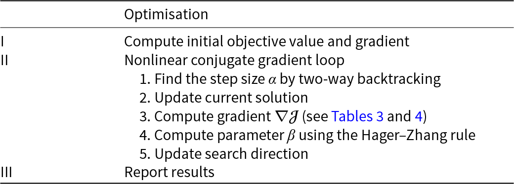
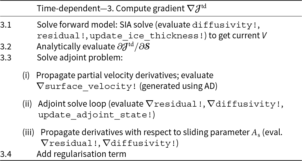
In this section, we describe the numerical implementation of the snapshot and time-dependent inversion approaches, along with the employed algorithms, which are summarised in Tables 2–4. To reconstruct the distribution of the sliding parameter  $ A_{\mathrm{s}} $, we use a gradient-based optimisation algorithm from the nonlinear conjugate gradient family, which necessitates efficient computation of the gradients or derivatives of the objective function with respect to the parameter of interest.
Overview of the optimisation procedure which is identical for both the snapshot and the time-dependent workflow, with the exception of step II.3 to compute the gradient of the objective function
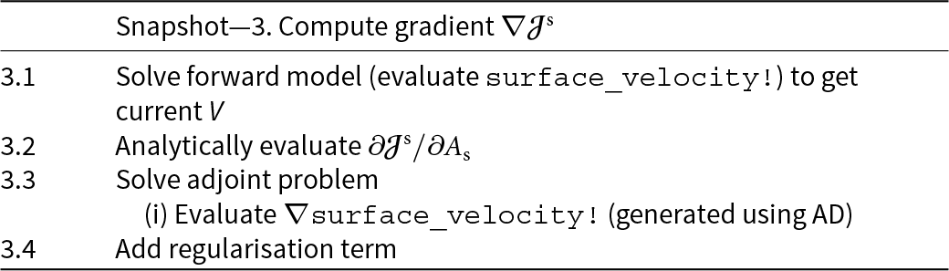
Overview of optimisation step II.3 of Table 2 for the snapshot case. The words typeset in typewriter font refer to function names in the provided model code, see Acknowledgements
Overview of optimisation step II.3 of Table 2 for the time-dependent case. The words typeset in typewriter font refer to function names in the provided model code, see Acknowledgements
In the snapshot inversion, the forward model consists of computing the SIA ice velocity V according to (9) while setting the ice thickness  $H = H_{\mathrm{obs}}$. This algebraic equation is linear in $A_{\mathrm{s}}$, which allows solving the inverse problem analytically in the absence of regularisation and computing the gradients of the objective function analytically as well. In this study, we use AD to compute gradients for the snapshot inversion nevertheless to keep the same implementation structure for both the snapshot and the time-dependent approaches. Since the forward model is just one function, we compute the gradient of $\mathcal{J}^\mathrm{s}$ in a single call to the AD tool.
In contrast to the snapshot inversion, the forward model in the time-dependent inversion case is the time-dependent SIA model. If using an explicit time integration to solve the SIA equations (11), (14) and (15), computing the gradient of the objective function  $\mathcal{J}^\mathrm{td}$ would require storing all the time steps in memory or using checkpointing algorithms, trading memory for redundant computations (Heimbach and Bugnion, Reference Heimbach and Bugnion2009). Given the sparsity of glacier observations in time, in this work, we use an implicit time integration instead, allowing us to advance the state of the simulation in one large time step equal to the gap between observations. Note that the presented approach would work for schemes taking several intermediate time steps at the expense of needing a scheme to store or recalculate results of the intermediate time steps. Using an AD tool, computing the gradient of the objective function $\mathcal{J}^\mathrm{td}$ with implicit time integration in the forward model can leverage the adjoint state method to avoid the substantial memory and computational overhead associated with differentiating the solver algorithm directly (Giles and Pierce, Reference Giles and Pierce2000). The adjoint state method requires solving one additional linear adjoint problem after solving the nonlinear forward problem (Reuber and others, Reference Reuber, Holbach and Räss2020).
We accelerate computations by specifically targeting Nvidia GPUs using the CUDA.jl package in Julia (Besard and others, Reference Besard, Churavy, Edelman and Sutter2019a, Reference Besard, Foket and De Sutter2019b) together with the AD tool Enzyme.jl (Moses and Churavy, Reference Moses and Churavy2020). In order to allow GPUs to deliver their full parallel performance, specific care needs to be taken regarding the choice of discretisation and algorithms. We use a conservative finite-difference scheme on a structured Cartesian grid, as it facilitates regular memory access, and use the APT method (Räss and others, Reference Räss, Utkin, Duretz, Omlin and Podladchikov2022). The APT method is a matrix-free iterative algorithm which involves only local updates at each point of the computational grid, trading the increased number of iterations for efficient massive parallelism. In Sandip and others Reference Sandip, Räss and Morlighem(2024), solving the shallow shelf approximation by APT method achieves 1.5 × speedup by leveraging GPU processing power. In our study, we apply the GPU-based APT method to solve both the forward and adjoint problems required to compute the gradient of the objective function for the time-dependent inversion.
2.4.1. Optimisation algorithm
To minimise the objective function defined for the snapshot (3) and the time-dependent (5) cases, we use a modified version of the nonlinear conjugate gradient method developed by Hager and Zhang Reference Hager and Zhang(2005). The optimisation procedure, summarised in Table 2, consists of two steps: (i) updating the solution  $\log\boldsymbol{A}_{\mathrm{s}}$ with the gradient of the objective function $\nabla\mathcal{J}$ using a suitable step size α and (ii) using the Hager–Zhang rule to update the search direction. We perform the updates in the log space to avoid negative values and more accurately span the expected range of values for $A_{\mathrm{s}}$:
 \begin{gather}
\log\boldsymbol{A}_{\mathrm{s}}^{k+1} = \log\boldsymbol{A}_{\mathrm{s}}^{k} + \alpha^k \boldsymbol{p}^k ,
\end{gather}
\begin{gather}
\log\boldsymbol{A}_{\mathrm{s}}^{k+1} = \log\boldsymbol{A}_{\mathrm{s}}^{k} + \alpha^k \boldsymbol{p}^k ,
\end{gather}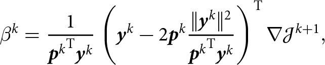 \begin{gather}
\beta^k = \frac{1}{{\boldsymbol{p}^k}^\mathrm{T} \boldsymbol{y}^k}\left(\boldsymbol{y}^k - 2\boldsymbol{p}^k\frac{\|\boldsymbol{y}^k\|^2}{{\boldsymbol{p}^k}^\mathrm{T} \boldsymbol{y}^k}\right)^\mathrm{T}\nabla\mathcal{J}^{k+1},
\end{gather}
\begin{gather}
\beta^k = \frac{1}{{\boldsymbol{p}^k}^\mathrm{T} \boldsymbol{y}^k}\left(\boldsymbol{y}^k - 2\boldsymbol{p}^k\frac{\|\boldsymbol{y}^k\|^2}{{\boldsymbol{p}^k}^\mathrm{T} \boldsymbol{y}^k}\right)^\mathrm{T}\nabla\mathcal{J}^{k+1},
\end{gather}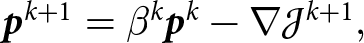 \begin{gather}
\boldsymbol{p}^{k+1} = \beta^k\boldsymbol{p}^{k} - \nabla\mathcal{J}^{k+1},
\end{gather}
\begin{gather}
\boldsymbol{p}^{k+1} = \beta^k\boldsymbol{p}^{k} - \nabla\mathcal{J}^{k+1},
\end{gather} where k is the iteration index, α k is the step size, pk is the search direction, β is the parameter computed using the Hager–Zhang rule (Hager and Zhang, Reference Hager and Zhang2005),  $\nabla\mathcal{J}^{k+1}$ is the gradient of the objective function with respect to $\log \boldsymbol{A}_{\mathrm{s}}^{k+1}$ and $\boldsymbol{y}^k = \nabla\mathcal{J}^{k+1} - \nabla\mathcal{J}^{k}$. Here we use bold symbols as all the quantities are vectors with components corresponding to grid points of the computational domain.
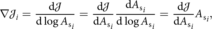
To compute the gradient  $\nabla\mathcal{J}$ with respect to $\log\boldsymbol{A}_{\mathrm{s}}$, we use the chain rule analytically:
 \begin{equation}
\nabla{\mathcal{J}}_i = \frac{\mathrm{d}\mathcal{J}}{\mathrm{d}\log {A_{\mathrm{s}}}_i}
= \frac{\mathrm{d}\mathcal{J}}{\mathrm{d}{A_{\mathrm{s}}}_i}\frac{\mathrm{d}{A_{\mathrm{s}}}_i}{\mathrm{d}\log {A_{\mathrm{s}}}_i}
= \frac{\mathrm{d}\mathcal{J}}{\mathrm{d}{A_{\mathrm{s}}}_i}{A_{\mathrm{s}}}_i,
\end{equation}
\begin{equation}
\nabla{\mathcal{J}}_i = \frac{\mathrm{d}\mathcal{J}}{\mathrm{d}\log {A_{\mathrm{s}}}_i}
= \frac{\mathrm{d}\mathcal{J}}{\mathrm{d}{A_{\mathrm{s}}}_i}\frac{\mathrm{d}{A_{\mathrm{s}}}_i}{\mathrm{d}\log {A_{\mathrm{s}}}_i}
= \frac{\mathrm{d}\mathcal{J}}{\mathrm{d}{A_{\mathrm{s}}}_i}{A_{\mathrm{s}}}_i,
\end{equation} where the products are calculated element-wise, i.e. without summation over the grid point index i. We compute the first term in Eqn (19) using AD, and then multiply the result by  $A_{\mathrm{s}}$ before passing the gradient to the optimisation routine.
We implemented a two-way backtracking line search to compute the step size α k which satisfies the Armijo–Goldstein condition (Armijo, Reference Armijo1966):
 \begin{equation}
\mathcal{J}(\boldsymbol{A}_{\mathrm{s}}^{k+1}) \leq \mathcal{J}(\boldsymbol{A}_{\mathrm{s}}^{k}) + m\,\alpha^k\, {\nabla\mathcal{J}^k}^\mathrm{T}\boldsymbol{p}^k,
\end{equation}
\begin{equation}
\mathcal{J}(\boldsymbol{A}_{\mathrm{s}}^{k+1}) \leq \mathcal{J}(\boldsymbol{A}_{\mathrm{s}}^{k}) + m\,\alpha^k\, {\nabla\mathcal{J}^k}^\mathrm{T}\boldsymbol{p}^k,
\end{equation} where  $m \in (0; 1)$ is a parameter which controls the sufficient decrease in the objective function $\mathcal{J}$ along the search direction pk. In this study, we set $m = 1/10$.
To actually calculate α k, we did not use the line search from Hager and Zhang Reference Hager and Zhang(2005), as it requires evaluating the gradient multiple times, which involves solving the adjoint system in the case of time-dependent inversion, and instead use the simpler two-way backtracking of Nocedal and Wright Reference Nocedal and Wright1999, which results in sufficiently fast convergence.
2.4.2. Forward model
We approximate the time derivative  $\partial H / \partial t$ (11) with an implicit backward Euler scheme and substitute the expression for q (15), which yields:
 \begin{equation}
\frac{H - H_\mathrm{old}}{\Delta t} = \nabla\cdot \left(D\nabla S\right) + \dot{b} ,
\end{equation}
\begin{equation}
\frac{H - H_\mathrm{old}}{\Delta t} = \nabla\cdot \left(D\nabla S\right) + \dot{b} ,
\end{equation} where  $H_\mathrm{old}$ is the ice thickness at the beginning of the modelled time period. Equation (21) is a nonlinear diffusion equation for the surface elevation S, or, equivalently, for the ice thickness $H = S - B$, since the bedrock elevation B is fixed in this study.
We solve (21) using the APT method (Räss and others, Reference Räss, Utkin, Duretz, Omlin and Podladchikov2022). We define the residual  $\mathcal{R}_\mathrm{f}$ of the forward problem upon rearranging terms from (21):
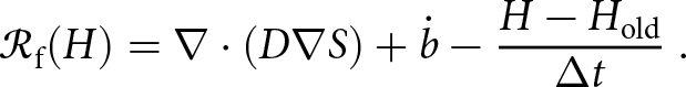 \begin{equation}
\mathcal{R}_\mathrm{f}(H) = \nabla \cdot \left(D \nabla S\right) + \dot{b} - \frac{H - H_\mathrm{old}}{\Delta t} ~.
\end{equation}
\begin{equation}
\mathcal{R}_\mathrm{f}(H) = \nabla \cdot \left(D \nabla S\right) + \dot{b} - \frac{H - H_\mathrm{old}}{\Delta t} ~.
\end{equation}According to the APT method, we introduce a two-step update procedure:
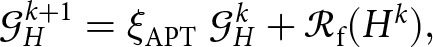 \begin{align}
\mathcal{G}_H^{k+1} &= \xi_\mathrm{APT} \; \mathcal{G}_H^{k} + \mathcal{R}_\mathrm{f}(H^{k}),
\end{align}
\begin{align}
\mathcal{G}_H^{k+1} &= \xi_\mathrm{APT} \; \mathcal{G}_H^{k} + \mathcal{R}_\mathrm{f}(H^{k}),
\end{align}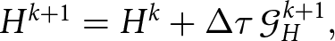 \begin{align}
H^{k+1} &= H^k + \Delta \tau \; \mathcal{G}_H^{k+1},
\end{align}
\begin{align}
H^{k+1} &= H^k + \Delta \tau \; \mathcal{G}_H^{k+1},
\end{align} where k is the APT iteration index,  $\mathcal{G}_{H}$ is the update rate of H, $\xi_\mathrm{APT} \in \left[0, 1\right]$ is the damping parameter leading to improved convergence (Räss and others, Reference Räss, Utkin, Duretz, Omlin and Podladchikov2022) and $\Delta \tau$ is the pseudo-time step size. At the first iteration, i.e. when k = 0, we set $\mathcal{G}_H^0 = \mathcal{R}_\mathrm{f}(H^0)$ and $H^0 = H_\mathrm{old}$.
We compute the pseudo-time step  $\Delta \tau$ by performing the linearised von Neumann stability analysis on the diffusion equation (21):
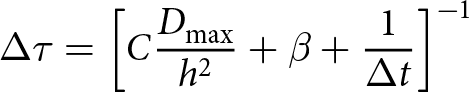 \begin{equation}
\Delta \tau = \left[C\frac{D_\mathrm{max}}{h^2} + \beta + \frac{1}{\Delta t}\right]^{-1}
\end{equation}
\begin{equation}
\Delta \tau = \left[C\frac{D_\mathrm{max}}{h^2} + \beta + \frac{1}{\Delta t}\right]^{-1}
\end{equation} where C is the stability parameter,  $D_\mathrm{max}$ is the maximum value of the diffusion coefficient D in space and h is the spacing of the computational grid. We stop the iterative procedure when the $L_\infty$-norm of the relative error drops below the defined tolerance, i.e. when $\| H^k - H^{k-1} \|_\infty / \| H^k \|_\infty \lt \epsilon_\mathrm{tol}$, where $\epsilon_\mathrm{tol} = 10^{-8}$ is the solver tolerance.
2.4.3. Automatic differentiation
AD provides a general approach to compute derivatives of almost arbitrary code by decomposing the source into primitive expressions, for which the derivative rules are known, and propagating these derivatives during the code execution. The benefit of AD compared to calculating derivatives using a finite difference approximation is the absence of truncation errors, and higher performance since finite differences require at least two function evaluations. Compared to manual or symbolic differentiation, apart from the obvious advantage of not having to perform symbolic computations, AD can provide more stable results in certain cases (Griewank and Walther, Reference Griewank and Walther2008).
AD has typically two distinct modes of derivatives propagation: forward mode and reverse mode (Giering and Kaminski, Reference Giering and Kaminski1998). Here, we are using the reverse mode, which is to accumulate the derivatives starting from the end of the function. It is more efficient for functions with more inputs than outputs (Moses and others, Reference Moses, Churavy, Paehler, Hückelheim, Narayanan, Schanen and Doerfert2021, Reference Moses2022), which is the case in our study, since the objective functional  $\mathcal{J}$ maps the vector with a component for each grid point to a scalar value.
In this study, we use Enzyme (Moses and Churavy, Reference Moses and Churavy2020), a high-performance AD compiler plugin for the LLVM compiler framework (Lattner, Reference Lattner2002) capable of synthesising gradients of programs expressed in the LLVM intermediate representation. The main benefit of working at the compiler level is the ability to differentiate the code after optimisation, resulting in substantial speedups compared to working on the source code level. Enzyme is one of the few existing AD tools that allows differentiating GPU code. Enzyme’s Julia interface, Enzyme.jl, makes it possible to differentiate GPU code written in a high-level language.
2.4.4. Adjoint problem
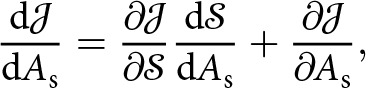
We compute the derivatives of the discrete objective functions reported by (3) and (5), which are needed in the optimisation procedure (16)–(19), using AD. The gradient, computed according to (19) in the inversion procedure, can be expanded using the chain rule as:
 \begin{equation}
\frac{\mathrm{d}\mathcal{J}}{\mathrm{d}A_{\mathrm{s}}} = \frac{\partial \mathcal{J}}{\partial \mathcal{S}}\frac{\mathrm{d} \mathcal{S}}{\mathrm{d} A_{\mathrm{s}}} + \frac{\partial \mathcal{J}}{\partial A_{\mathrm{s}}},
\end{equation}
\begin{equation}
\frac{\mathrm{d}\mathcal{J}}{\mathrm{d}A_{\mathrm{s}}} = \frac{\partial \mathcal{J}}{\partial \mathcal{S}}\frac{\mathrm{d} \mathcal{S}}{\mathrm{d} A_{\mathrm{s}}} + \frac{\partial \mathcal{J}}{\partial A_{\mathrm{s}}},
\end{equation} where  $\mathcal{S} = \{H, V\}$ is the solution vector including both ice thickness and velocity. Note that the term $\mathrm{d} \mathcal{S}/\mathrm{d} A_{\mathrm{s}}$ is dependent on the full forward model calculation and thus may require the above-mentioned storage of intermediate results in the reverse-mode AD evaluation.
However, in the snapshot case, the forward model is computed with just the algebraic evaluation of the surface velocity V from (9). Because the evaluation does not involve an iterative solver, the derivative calculation of  $\mathrm{d} \mathcal{S}/\mathrm{d} A_{\mathrm{s}}$ via reverse-mode AD is straightforward and efficient as no intermediate results are generated.
Conversely, the time-dependent inversion requires solving the differential equation (11) for a given time span. The forward model, after discretising the time derivative, is a nonlinear degenerate elliptic equation, which we solve using an implicit time integration with the iterative APT algorithm described above. Thus, the reverse-mode AD calculation would require storing all intermediate iteration steps since the result of an iterative solve formally depends on the initial guess. While feasible for small problems based on 1-D models such as flowline models, for high-resolution 2-D and 3-D models, the amount of memory required to store intermediate results becomes prohibitively large.
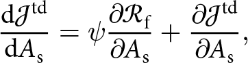
However, the result of a converged iterative solve only varies for changes in the initial guess in a small range within the nonlinear solver tolerance, and thus we can remove the dependence on the initial guess and with it the need to save the intermediate calculations. Using this approach requires modifications to the AD workflow, which go under the name of adjoint state method. In this method, the gradient given by (26) is calculated with:
 \begin{equation}
\frac{\mathrm{d}\mathcal{J}^\mathrm{td}}{\mathrm{d} A_{\mathrm{s}}} = \psi \frac{\partial \mathcal{R}_\mathrm{f}}{\partial A_{\mathrm{s}}} + \frac{\partial \mathcal{J}^\mathrm{td}}{\partial A_{\mathrm{s}}},
\end{equation}
\begin{equation}
\frac{\mathrm{d}\mathcal{J}^\mathrm{td}}{\mathrm{d} A_{\mathrm{s}}} = \psi \frac{\partial \mathcal{R}_\mathrm{f}}{\partial A_{\mathrm{s}}} + \frac{\partial \mathcal{J}^\mathrm{td}}{\partial A_{\mathrm{s}}},
\end{equation} where the adjoint state  $\psi$ can be calculated with the adjoint equation:
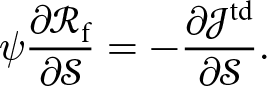 \begin{equation}
\psi \frac{\partial \mathcal{R}_\mathrm{f}}{\partial \mathcal{S}} = -\frac{\partial \mathcal{J}^\mathrm{td}}{\partial \mathcal{S}}.
\end{equation}
\begin{equation}
\psi \frac{\partial \mathcal{R}_\mathrm{f}}{\partial \mathcal{S}} = -\frac{\partial \mathcal{J}^\mathrm{td}}{\partial \mathcal{S}}.
\end{equation} Note that now the gradient can be calculated without employing the solution of the forward model and thus without needing memory-intensive storage for reverse-mode AD at the cost of a relatively cheap linear solve of (28). Further note that formally the residual  $\mathcal{R}_\mathrm{f}$ depends only on H according to (22), therefore, $\partial \mathcal{R}_\mathrm{f} / \partial V = 0$. In the numerical implementation, we do not include the unnecessary degrees of freedom to save computational resources, but here we keep the extended notation for consistency.
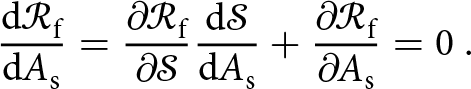
To prove that the gradient  $\mathrm{d} {\mathcal{J}}_\mathrm{td} / \mathrm{d} A_{\mathrm{s}}$ computed using (27) is consistent with (26), we use the fact that at the solution, the residual of the forward problem vanishes for all $A_{\mathrm{s}}$, i.e. $\mathcal{R}_\mathrm{f}(\mathcal{S}) = 0$. Computing the derivative with respect to $A_{\mathrm{s}}$ and using the chain rule yields
 \begin{equation}
\frac{\mathrm{d} \mathcal{R}_\mathrm{f}}{\mathrm{d} A_{\mathrm{s}}} = \frac{\partial \mathcal{R}_\mathrm{f}}{\partial \mathcal{S}} \frac{\mathrm{d} \mathcal{S}}{\mathrm{d} A_{\mathrm{s}}} + \frac{\partial \mathcal{R}_\mathrm{f}}{\partial A_{\mathrm{s}}} = 0~.
\end{equation}
\begin{equation}
\frac{\mathrm{d} \mathcal{R}_\mathrm{f}}{\mathrm{d} A_{\mathrm{s}}} = \frac{\partial \mathcal{R}_\mathrm{f}}{\partial \mathcal{S}} \frac{\mathrm{d} \mathcal{S}}{\mathrm{d} A_{\mathrm{s}}} + \frac{\partial \mathcal{R}_\mathrm{f}}{\partial A_{\mathrm{s}}} = 0~.
\end{equation} Solving this for  $\partial \mathcal{R}_\mathrm{f} / \partial A_{\mathrm{s}}$, inserting into (27) and further simplifying with (28) transforms (27) into (26) and thus completes the proof.
We solve (28) using the same APT procedure as for the forward problem, by employing the two-stage procedure, updating the rate of change of the variable  $\psi$ with the damped residual, and then updating $\psi$ with the pseudo-time step $\Delta \tau$:
 \begin{align}
\mathcal{G}_\psi^{k+1} &= \xi_\mathrm{APT} \; \mathcal{G}_\psi^{k} + \mathcal{R}_\mathrm{a}(\psi^k),
\end{align}
\begin{align}
\mathcal{G}_\psi^{k+1} &= \xi_\mathrm{APT} \; \mathcal{G}_\psi^{k} + \mathcal{R}_\mathrm{a}(\psi^k),
\end{align}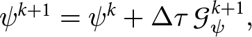 \begin{align}
\psi^{k+1} &= \psi^k + \Delta \tau \; \mathcal{G}_\psi^{k+1},
\end{align}
\begin{align}
\psi^{k+1} &= \psi^k + \Delta \tau \; \mathcal{G}_\psi^{k+1},
\end{align} where  $\mathcal{G}_\psi$ is the rate of change of $\psi$. We use the same pseudo-time step $\Delta \tau$ reported by (25) for the adjoint problem since the spectral properties of the adjoint operator are the same as those of the linearised forward operator. We summarise the steps to compute the gradient of the time-dependent objective function $\nabla \mathcal{J}^\mathrm{td}$ in Table 4.
We investigate two different model configurations for which we will perform snapshot and time-dependent inversions. The first model configuration uses synthetic glacier geometry and SMB. The second model configuration uses elevation, velocity and SMB data from the Aletsch glacier in the Swiss Alps. Hereafter, we describe the initial conditions and model configurations. The values of the parameters used in both the synthetic and Aletsch case are listed in Table 5.
Parameters for the synthetic and Aletsch configurations. Parameters not applicable for the Aletsch configuration are marked with ‘–’
In a synthetic model set-up, we compare the results using different weights  $\left(\omega^n_V, \omega^n_H\right)$ in the objective function of the time-dependent inversion (5). We use the Aletsch glacier configuration over the hydrological years 2016–17 to assess how using snapshot versus time-dependent inversion results impact surface velocity distributions and geometry changes and perform a mesh convergence test for both the snapshot and time-dependent cases.
2.5. Synthetic glacier
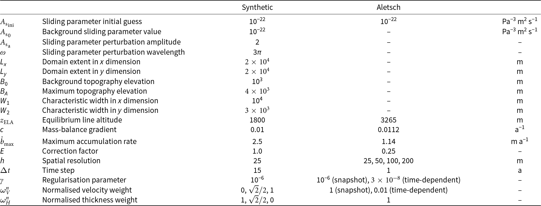
For the synthetic case, we generate a synthetic bed topography inspired by what Visnjevic and others Reference Visnjevic, Herman and Podladchikov(2018) suggested for benchmarking purposes and define the bedrock B as a combination of two Gaussian shapes (Fig. 1a):
 \begin{align}
B &= B_0 + \frac{B_\mathrm{A}}{2}
\left\{\exp\left[-\left(\frac{x}{W_1}\right)^2 -
\left(\frac{y}{W_2}\right)^2\right]\right. \nonumber\\
&\left.\quad+\,\exp\left[-\left(\frac{x}{W_2}\right)^2
- \left(\frac{y}{W_1}\right)^2\right]
\right\},
\end{align}
\begin{align}
B &= B_0 + \frac{B_\mathrm{A}}{2}
\left\{\exp\left[-\left(\frac{x}{W_1}\right)^2 -
\left(\frac{y}{W_2}\right)^2\right]\right. \nonumber\\
&\left.\quad+\,\exp\left[-\left(\frac{x}{W_2}\right)^2
- \left(\frac{y}{W_1}\right)^2\right]
\right\},
\end{align}Synthetic glacier configuration. (a) Bedrock elevation and glacier outline; (b) initial (steady) state ice velocity magnitude; (c) initial (steady) state ice thickness distribution; (d) perturbed sliding coefficient distribution; (e) synthetic ice velocity magnitude after  $\Delta t = 15$ years; (f) synthetic ice thickness after $\Delta t = 15$ years.
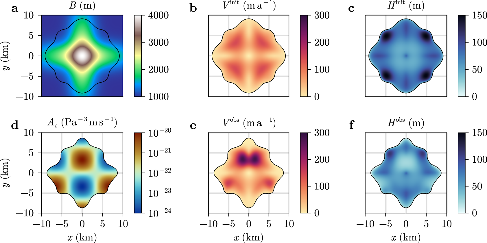
where B 0 is the background elevation,  $B_\mathrm{A}$ is the mountain height, W 1 and W 2 are characteristic widths, and x and y are the horizontal coordinates.
With this configuration, using a uniform distribution of the sliding coefficient  $A_{\mathrm{s}} = A_{\mathrm{s}_0}$ and the simple altitude-dependent SMB model (13), we run the forward model to steady state, setting $\Delta t = \infty$ in (21), in order to generate synthetic initial ice thickness $H^\mathrm{init}$ (Fig. 1c) and velocity fields $V^\mathrm{init}$ (Fig. 1b).
We then define a synthetic perturbation of the sliding parameter  $A_{\mathrm{s}}^\mathrm{syn}$:
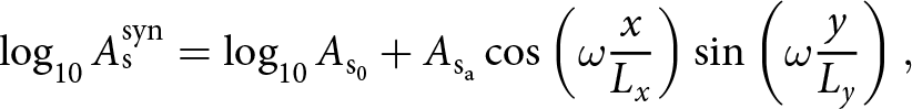 \begin{equation}
\log_{10} A_{\mathrm{s}}^\mathrm{syn} = \log_{10} A_{\mathrm{s}_0} + A_{\mathrm{s}_\mathrm{a}}
\cos\left(\omega\frac{x}{L_x}\right)
\sin\left(\omega\frac{y}{L_y}\right),
\end{equation}
\begin{equation}
\log_{10} A_{\mathrm{s}}^\mathrm{syn} = \log_{10} A_{\mathrm{s}_0} + A_{\mathrm{s}_\mathrm{a}}
\cos\left(\omega\frac{x}{L_x}\right)
\sin\left(\omega\frac{y}{L_y}\right),
\end{equation} where  $A_{\mathrm{s}_0}$ is the background value, $A_{\mathrm{s}_\mathrm{a}}$ is the perturbation amplitude in log-space and ω is the perturbation wavelength. Lx and Ly are the model extents in the x and y directions, respectively. Additionally, we perturb $z_\mathrm{ELA}$ with a step increase of 20%. We then use $H^\mathrm{init}$ as the initial condition for a forward SIA run with the perturbed parameters over a time span of 15 years with one time step of equal length to generate the synthetic thickness $H^{\mathrm{obs}}$ (Fig. 1f) and velocity fields $V^{\mathrm{obs}}$ (Fig. 1e).
2.6. Aletsch glacier
As the second configuration, we use the Aletsch glacier, the largest glacier in the Alps (Fig. 2). With this configuration, we show that our inversion framework is capable of inferring a spatially variable sliding coefficient  $A_{\mathrm{s}}$ by using surface velocity V and changes in the ice geometry H as observational data during the hydrological years 2016–17. To generate the input data for the Aletsch glacier, we process elevation (bedrock and surface), ice surface velocity and SMB data.
Aletsch glacier configuration. (a) Bedrock elevation and glacier outline; (b) measured ice velocity magnitude for the years 2016–17; (c) mass-balance mask; (d) reconstructed ice thickness distribution for the year 2016 interpolating data from years 2009 and 2017; (e) change in ice thickness in the hydrological years 2016–17; (f) surface mass-balance model depicting  $\dot b$ as a function of altitude z showing data points and fitted piece-wise linear model.
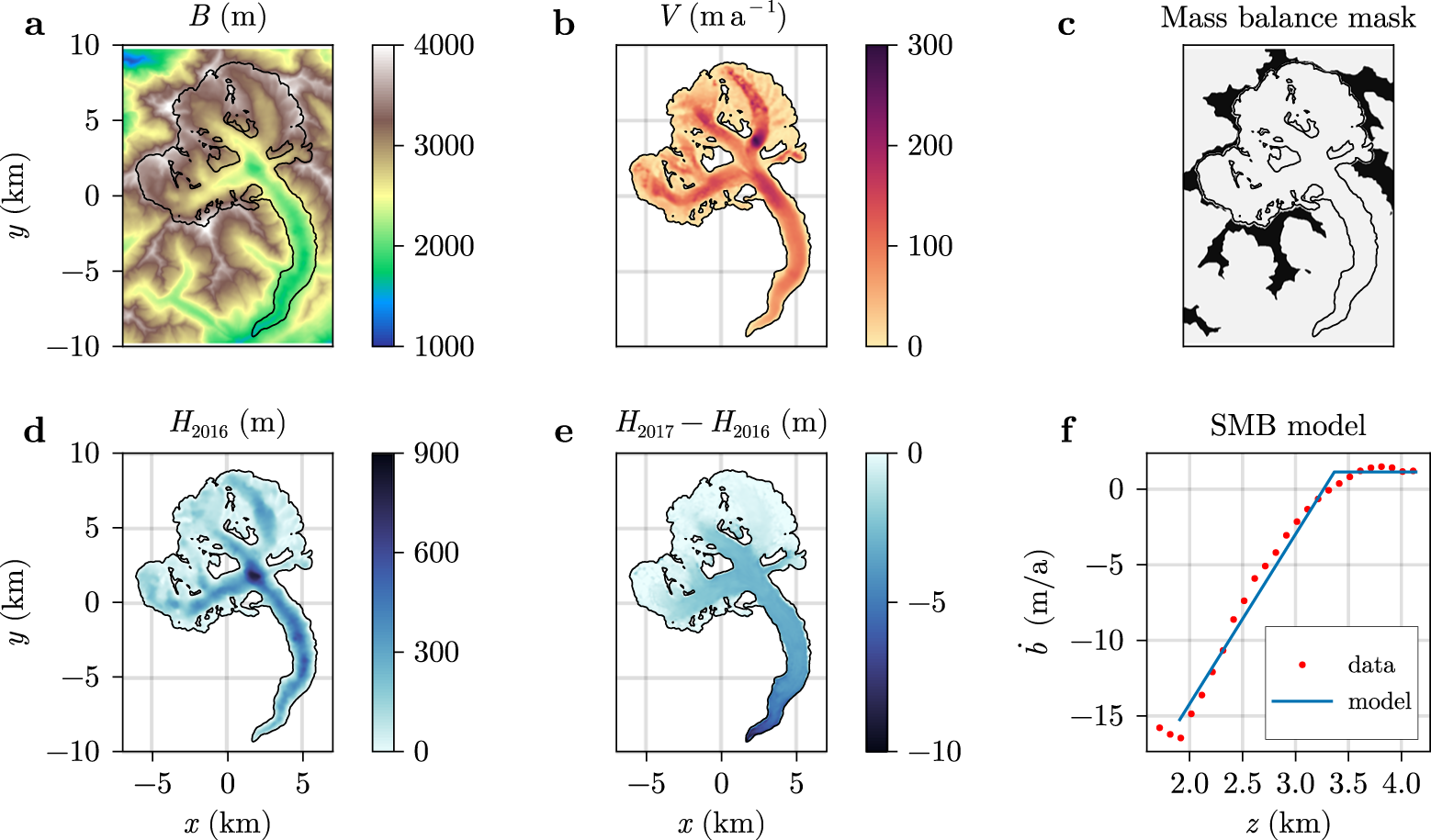
We extract bedrock and surface elevation from Grab and others Reference Grab(2021) combined with swissALTI3D (Swiss Federal Office of Topography swisstopo, 2022) in ice-free regions (Fig. 2a). Since we do not have ice surface elevation data for the year 2016, we create it by assuming a linear variation between the years 2009 and 2017, for which digital elevation models are available. We then compute ice thickness from bedrock and ice surface elevation (Fig. 2d,e).
We extract annual ice surface velocity data V from Rabatel and others Reference Rabatel, Ducasse, Millan and Mouginot2023 for the hydrological years 2016–17 (Fig. 2b). We replace missing values with zeros to run the numerical codes and resample the data to match the bedrock extent and resolution using cubic spline interpolation. We also mask the velocity data with the ice mask, ensuring consistency among velocity and ice thickness datasets.
We extract SMB data for the 2016–17 hydrological year (Fig. 2f) from GLAMOS - Glacier Monitoring Switzerland (2023) to fit our simple altitude-dependent parameterisation (13). One caveat of using a simple altitude-dependent SMB model is that it does not account for lateral variations in mass balance, which may result in nonzero ice thickness in regions where the observed surface is ice-free. Here, we use a distributed correction for the mass balance by introducing a mass-balance mask (Fig. 2c), which removes ice accumulation in regions where the observed ice thickness is zero.
3. Results
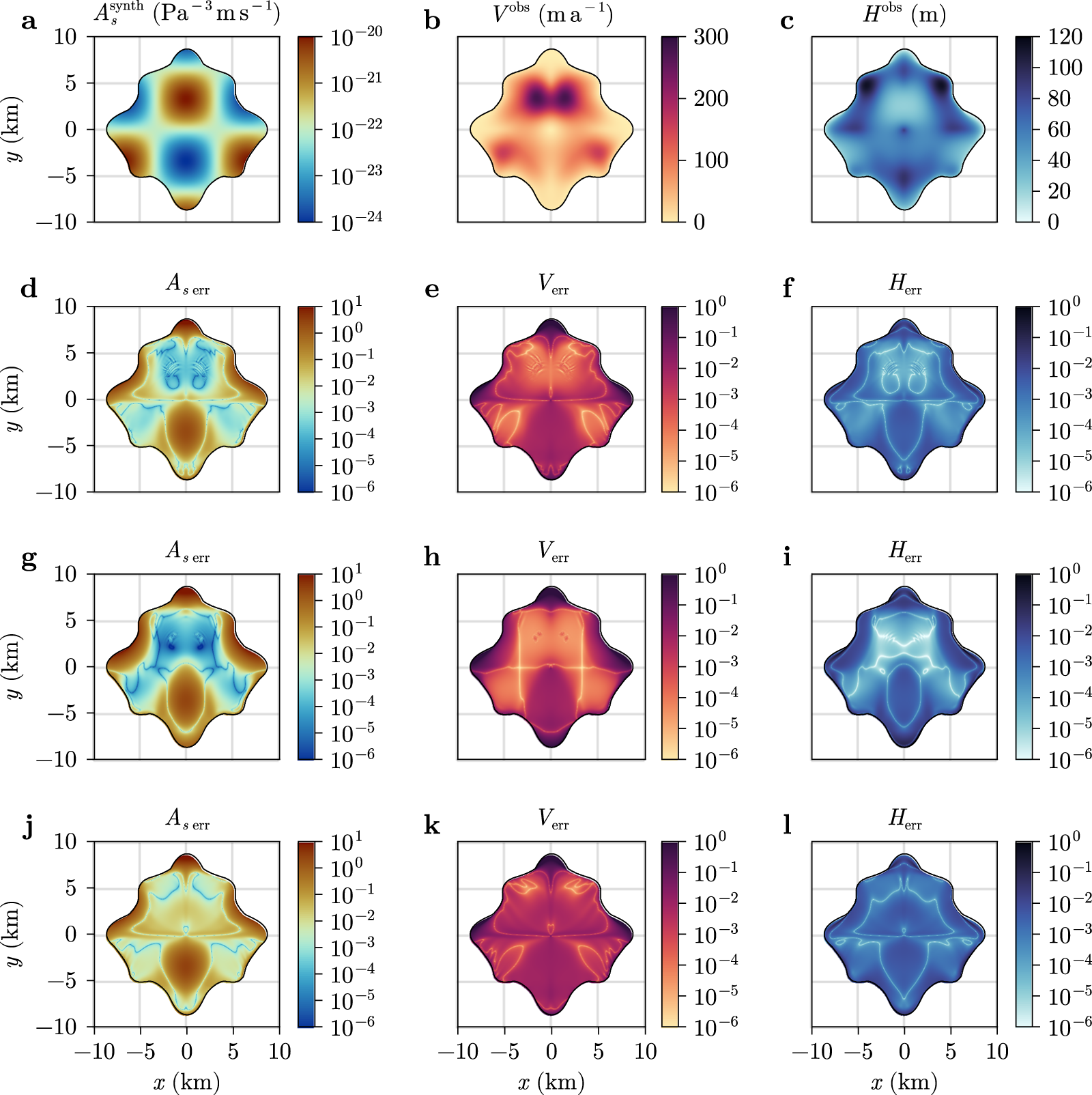
3.1. Time-dependent inversion on synthetic geometry
We perform a time-dependent inversion to reconstruct the spatial distribution of the basal sliding parameter  $A_{\mathrm{s}}$ in a synthetic model set-up (Fig. 1). We aim at reconstructing the synthetic sliding coefficient distribution (Fig. 3a) using synthetic velocity observations $V^{\mathrm{obs}}$ (Fig. 3b) and ice geometry observations $H^{\mathrm{obs}}$ (Fig. 3c) which were generated by running the forward SIA model with $A_{\mathrm{s}}^\mathrm{syn}$ (33) for one time step of $\Delta t = 15$ years. We achieve this inversion by minimising the objective function (5) using the optimisation algorithm described above. We stop the optimisation procedure after 1000 iterations of the algorithm (Eqns (16)–(18)), ensuring convergence and achieving a reduction in the objective function by more than three orders of magnitude.
Time-dependent inversion of  $A_{\mathrm{s}}$ on synthetic set-up. (a) Synthetic basal sliding parameter distribution (ground truth to be reconstructed); (b) ice surface velocity distribution after $\Delta t = 15$ years (the observed ice velocity to be used in the objective function during reconstruction); (c) ice thickness and geometry after $\Delta t = 15$ years (the observed ice thickness to be used in the objective function during reconstruction); (d–f) time-dependent inversion of $A_{\mathrm{s}}$ using both $V^{\mathrm{obs}}$ and $H^{\mathrm{obs}}$ in the objective function setting $\omega^n_V=\omega^n_H$ (Eqns (6) and (7)); (g–i) time-dependent inversion of $A_{\mathrm{s}}$ using only $V^{\mathrm{obs}}$ in the objective function setting $\omega^n_H = 0$; (j–l) time-dependent inversion of $A_{\mathrm{s}}$ using only $H^{\mathrm{obs}}$ in the objective function setting $\omega^n_V = 0$. For the three inversion scenarios, we report comparison of reconstructed versus synthetic sliding parameter: $A_{\mathrm{s}\ \mathrm{err}} = \left|A_{\mathrm{s}} - A_{\mathrm{s}}^\mathrm{synth}\right|/A_{\mathrm{s}}^\mathrm{synth}$; (d, g, i) a comparison of reconstructed versus observed velocity $V_\mathrm{err} = \left|V - V^{\mathrm{obs}}\right| / V^{\mathrm{obs}}$; and (e, h, k) geometry (thickness) $H_\mathrm{err} = \left|H - H^{\mathrm{obs}}\right| / H^{\mathrm{obs}}$.
We have performed systematic numerical experiments to determine the values of regularisation parameter γ and normalised weights  $\omega_V^n$ and $\omega_H^n$. Since we do not include any artificial noise in the synthetic observations and parameters, and the synthetic distribution of sliding parameter $A_{\mathrm{s}}^\mathrm{synth}$ is sufficiently smooth, the value of γ does not affect the inversion results below a certain threshold $\gamma \approx 10^{-6}$, since there is an exact solution for $A_{\mathrm{s}}$. However, selecting γ values significantly smaller than 10−6 results in slower convergence of the implicit SIA solver due to the highly irregular intermediate distributions of $A_{\mathrm{s}}$.
Using any combination of weights for the velocity and ice thickness data accurately reconstructs the synthetic  $A_{\mathrm{s}}$ field in regions far from the ice margin, with the largest discrepancies occurring near the glacier boundaries. Inversion relying solely on synthetic velocity data, as shown in Figure 3g–i, achieves the best fit for the sliding parameter $A_{\mathrm{s}}$ within the glacier interior. However, near the boundaries, the reconstruction error increases to over 100%. Conversely, inversion using only synthetic ice thickness data, illustrated in Figure 3j–l, provides the most accurate fit near the ice margin but yields the poorest reconstruction quality within the glacier interior.
Finally, incorporating both ice thickness and velocity data with  $\omega_V^n = \omega_H^n$ in the time-dependent inversion offers a balanced approach between these two extremes. As demonstrated in Figure 3d–f, this hybrid time-dependent inversion reproduces the synthetic $A_{\mathrm{s}}$ field more effectively than the velocity-only inversion near the boundaries and outperforms the thickness-only inversion in the interior.
A possible explanation for this phenomenon is that, near the ice margin, the ice thickness H decreases rapidly, while the gradient  $\nabla S$ increases in magnitude, as described by (9). Consequently, the sensitivity of velocity V to changes in $A_{\mathrm{s}}$ diminishes towards the ice margin. In contrast, the ice thickness remains sensitive to variations in $A_{\mathrm{s}}$ near the glacier boundary. These results suggest that time-dependent inversions incorporating both velocity and thickness data in the objective function provide the most accurate reconstruction.
3.2. Time-dependent versus snapshot inversions for Aletsch glacier
In the following numerical experiments, we aim to assess the quality of the modelled surface velocity and ice thickness fields on Aletsch glacier for basal sliding distributions reconstructed using the snapshot and the time-dependent inversion strategies. We also investigate the impact of refining the spatial resolution in a mesh convergence experiment. In the time-dependent inversion, we run the forward model for  $\Delta t = 1$ year (2016–17). We stop both the snapshot and time-dependent optimisation procedures after 1000 iterations of the algorithm (Eqns (16)–(18)). In all cases, the objective function stopped decreasing further before reaching 1000 iterations.
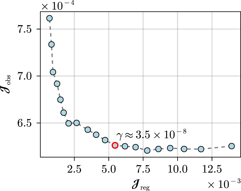
3.2.1. L-curve analysis
We use the L-curve method to empirically select the regularisation parameter γ in the inversion. We systematically perform multiple inversions with different values of γ within the range  $[5 \times 10^{-9};\ 5 \times 10^{-7}]$ and plot the corresponding values of the observational part ${\mathcal{J}}_{\mathrm{obs}}$ of the objective functional against the values of the regularisation component ${\mathcal{J}}_{\mathrm{reg}}$. These points geometrically form an L-shaped curve, where large values of ${\mathcal{J}}_{\mathrm{reg}}$ indicate overfitted solutions, and large values of ${\mathcal{J}}_{\mathrm{obs}}$ indicate excessively smoothed solutions. The corner of this L-curve identifies the optimal balance between fitting the data and applying regularisation. Figure 4 shows an example of an L-curve, where each point represents the result of a time-dependent inversion for the Aletsch glacier with a different value of γ. We have performed a similar analysis to determine the optimal range of the normalised weights of the contributions of the velocity and the ice thickness $\omega_V^n$ and $\omega_H^n$, respectively. The values of the parameters selected by the L-curve method are listed in Table 5.
L-curve for the time-dependent Aletsch inversion. The point corresponding to the optimal regularisation parameter  $\gamma \approx 3.5 \times 10^{-8}$ is highlighted in red.
3.2.2. Mesh convergence
In this section, we investigate mesh convergence by systematically running inversions to find the coarsest resolution at which the solution does not exhibit mesh dependence. The impact of refining the computational mesh on reconstructed  $A_{\mathrm{s}}$ for the Aletsch glacier configuration is assessed for both the time-dependent (Fig. 5a–d) and snapshot (Fig. 5e–f) inversions. The coarse grid with grid cell sizes of 200 m (Fig. 5a,e) does not capture finer structures that may impact the ice-flow velocity field. The finest grid, with grid cell sizes of 25 m (Fig. 5d,h), accurately captures variations in $A_{\mathrm{s}}$. The fact that the features and patterns do not significantly change for resolutions of 50 m and 25 m suggests that we achieved mesh convergence for discretisation using grid cell sizes of 25 m and motivates our numerical resolution choice throughout the paper.
Mesh convergence for the Aletsch glacier configuration for time-dependent (a–d) and snapshot (e–h) inversions showing the  $A_{\mathrm{s}}$ field. Spatial grid resolution refinement reducing from 200 m (a, e), 100 m (b, f), 50 m (c, g) and to 25 m for the highest resolution (d, h).
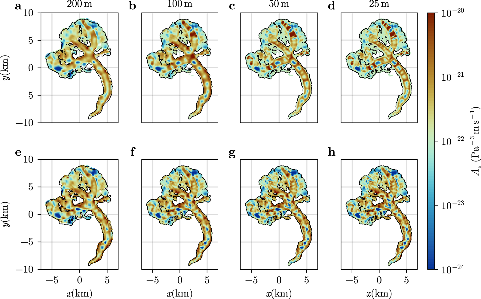
3.2.3. Reconstructed velocity field
We report the surface velocity distribution on the Aletsch glacier for the hydrological years 2016–17 using a spatial resolution of 25 m. We compare three inverted surface velocity distributions, shown in Figure 6b–d, to the observed surface velocity data taken from Rabatel and others (Reference Rabatel, Ducasse, Millan and Mouginot2023), shown in Figure 6a. In the snapshot case, the reported velocity field, shown in Figure 6b, is obtained by computing the SIA velocity from (9) for the reconstructed distribution of the sliding parameter  $A_{\mathrm{s}}$ (Fig. 5h), while keeping the glacier geometry set to the ice thickness distribution from Grab and others Reference Grab(2021). Discrepancies such as high-velocity patches and other artefacts are clearly visible when comparing the modelled velocity (Fig. 6b) to the observed velocity (Fig. 6a).
Observed and predicted ice surface velocity distribution for different inversion scenarios. (a) Observed distribution on the Aletsch glacier for the hydrological years 2016–17 (same as panel Figure 2b); (b) predicted distribution retrieved upon convergence of the snapshot inversion; (c) predicted distribution running the ice-flow solver for one time step of  $\Delta t = 1$ year using $A_{\mathrm{s}}$ reconstructed by the snapshot inversion; (d) predicted distribution from the time-dependent inversion.
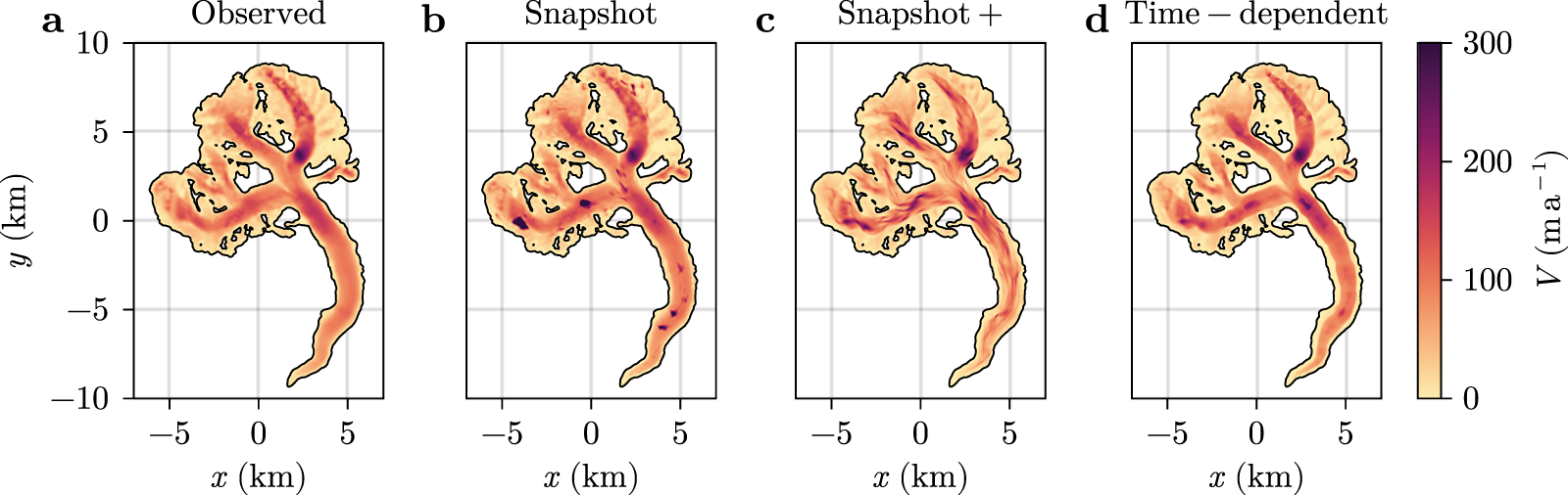
On the other side of the spectrum, performing time-dependent inversion for the 2016–17 period (Fig. 6d) provides a much better fit between modelled velocity and data (Fig. 6a) (see next subsection for the quantitative analysis). The corresponding reconstructed basal sliding distribution (Fig. 5d) for the time-dependent case features less high-frequency detail compared to the distribution of  $A_{\mathrm{s}}$ in the snapshot case (Fig. 5h).
As an additional case, we consider a scenario, which we call ‘Snapshot+’, where the distribution of the sliding parameter  $A_{\mathrm{s}}$ is taken from the snapshot inversion, but the velocity field is computed by running the forward SIA model for the time period 2016–17 with the same parameters as for the time-dependent inversion. This scenario is inspired by previously used combinations of inversion and spin-up to avoid transient shocks at the beginning of prognostic model runs e.g.
Gillet-Chaulet and others (Reference Gillet-Chaulet2012), Lipscomb and others (Reference Lipscomb, Leguy, Jourdain, Asay-Davis, Seroussi and Nowicki2021). We observe that the Snapshot+ model run delivers a slightly improved surface velocity field, as shown in Figure 6c, although being outperformed by the results from the time-dependent inversion.
$A_{\mathrm{s}}$ is taken from the snapshot inversion, but the velocity field is computed by running the forward SIA model for the time period 2016–17 with the same parameters as for the time-dependent inversion. This scenario is inspired by previously used combinations of inversion and spin-up to avoid transient shocks at the beginning of prognostic model runs e.g.
Gillet-Chaulet and others (Reference Gillet-Chaulet2012), Lipscomb and others (Reference Lipscomb, Leguy, Jourdain, Asay-Davis, Seroussi and Nowicki2021). We observe that the Snapshot+ model run delivers a slightly improved surface velocity field, as shown in Figure 6c, although being outperformed by the results from the time-dependent inversion.
3.2.4. Errors of velocity and ice thickness after inversion
Using the results of the snapshot and time-dependent inversion, we evaluate the difference between the observed surface velocity for the hydrological years 2016–17 and the modelled one, as well as the difference between observed surface elevation at the end of that hydrological year and the modelled one. The error is evaluated as the percent relative local difference between modelled and observed quantities  $\widehat V_\mathrm{err} = (V_{\mathrm{s}} - V^{\mathrm{obs}})/V^{\mathrm{obs}} \times 100\%$ and equivalently for the ice thickness H. Note that this is different from the synthetic case where we computed fractions and not percent (Fig. 3).
We report better quality velocity fields, thus lower  $\widehat V_\mathrm{err}$, for the time-dependent case (Fig. 7a), compared to the snapshot case (Fig. 7b). Averaged over the whole glacier, $\widehat V_\mathrm{err}$ is $-26\%$ and $-13\%$ for the snapshot and time-dependent inversion, respectively. This contrasts with the thickness error, $\widehat H_\mathrm{err}$, which is slightly lower for the snapshot than for the time-dependent inversion (Fig. 7c,d). However, the glacier-averaged thickness errors, which are between −3 and $-4\%$, are significantly lower for both types of inversions than either of the velocity errors.
Inversion errors for Aletsch glacier reported as percent error relative to the locally observed quantity. Error in velocity (top row, a, b); and in geometry (ice thickness) (bottom row, c, d); errors for Snapshot+, i.e. snapshot inversion results advanced forward in time by 1 year (left column, a, c); and time-dependent inversions (right column, b, d). Note that (a) corresponds to the relative difference of panel (c) and (a) of Figure 6 and (b) of panel (d) and (a).
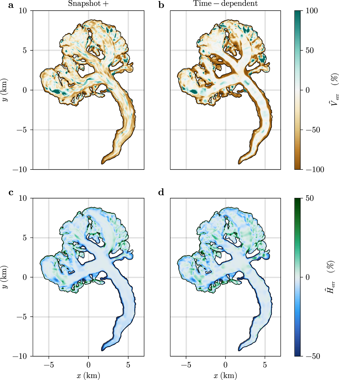
In both Snapshot+ and time-dependent cases, the relative error in velocity is larger closer to the glacier margins than closer to the central flowline. The main reason for that is the magnitude of velocity is small near margins, and small mismatches result in large relative errors. For time-dependent case, these relative errors are larger than for the Snapshot+ case. One possible explanation is the inconsistency between the ice surface and velocity datasets, which leads to locally contradicting optimisation objectives, especially near the margins where the ice thickness changes abruptly.
3.3. Performance
We evaluate the performance improvements achieved by enabling GPU acceleration in our code by benchmarking the forward SIA solver of Glaide.jl against a parallel CPU code PISM (Winkelmann and others, Reference Winkelmann, Martin, Haseloff, Albrecht, Bueler, Khroulev and Levermann2011). The benchmark involves a 100 years forward simulation of our synthetic glacier case without sliding, tested at spatial resolutions (grid cell sizes) of 25, 50, 100 and 125 m. PISM is chosen for comparison due to its reliance on finite differences, inclusion of a SIA ice-flow solver, and support for distributed memory parallelisation on CPUs using MPI, which maximises CPU compute capabilities. Wall-time is used as the primary performance metric, as it reflects practical concerns regarding time-to-solution. More complex metrics would neither aid the reader nor enhance the comparison of fundamentally different computing processors. Benchmark runs were conducted on HPC hardware, specifically a single Nvidia A100 GPU (40 GB) and an AMD EPYC 7282 16-Core CPU, with peak memory bandwidths (data transfer speed between memory and processor) of approximately 1555 GB/s and 85 GB/s, respectively. Note that the CPU’s monetary value is about an order of magnitude smaller than the GPU’s.
The PISM SIA solver employs an explicit time-stepping scheme with step sizes adjusted to satisfy the CFL condition. In contrast, Glaide.jl uses implicit time steps  $\Delta t = 2$ years. Simulations were conducted for the four resolutions, and wall-times were recorded. GPU-accelerated Glaide.jl runs completed within seconds, while MPI-parallel PISM simulations required hours for the finest tested grid resolution of 25 m (array size $800 \times 800$). The GPU implementation achieved speedups of up to three orders of magnitude in the 25 m case (Table 6). To assess accuracy, the L 2 error norm of the scaled difference $\Delta H = |H^\mathrm{Glaide.jl} - H^\mathrm{PISM}| / |\max(H^\mathrm{Glaide.jl})|$ was calculated at a 50 m resolution, yielding $||\Delta H||_2 = 2.66\times10^{-5}$.
Solver performance comparison. We use wall-time as a metric to compare the time it takes to solve the forward problem without sliding on our synthetic geometry. The Glaide.jl code runs on a single Nvidia A100 GPU, while the PISM code runs on 16 MPI ranks (16 cores) on a single data-centre AMD EPYC 7282 16-Core CPU
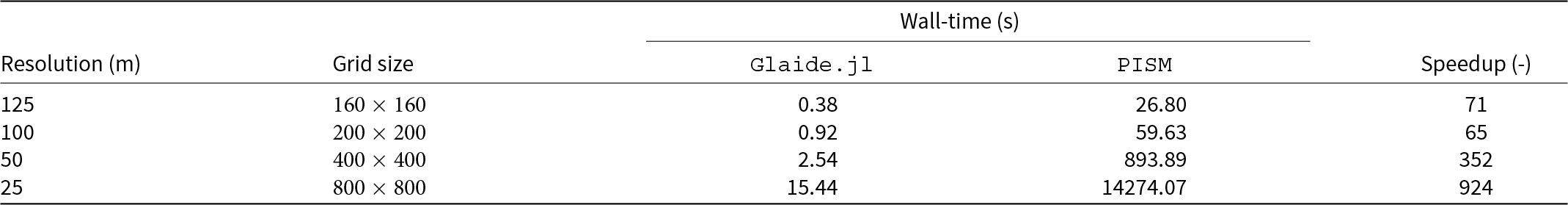
4. Discussion
The comparison between snapshot and time-dependent inversions for the Aletsch case highlights differences in the recovered surface velocities (Fig. 6) and associated basal sliding coefficient fields (Fig. 5d,h). The snapshot inversion tends to produce unrealistic distributions of  $A_{\mathrm{s}}$, particularly concerning lateral distribution and patchiness, resulting in significant errors in the modelled velocity field (Figs. 6c and 7a). Conversely, the time-dependent inversion incorporates changes in ice geometry and velocities over time, allowing, in a sense, limited nonlocal influences on ice velocity through evolving geometry. This yields less patchy results that better conform to the observed data. Nonetheless, the bed likely remains too slippery along the lateral margins. We identify two main factors affecting results of inversions, stemming from limitations of the forward model and the quality of datasets.
The first factor that could probably explain these unrealistic distributions of  $A_{\mathrm{s}}$ and the mismatches between the modelled and observed velocities is the absence of membrane stresses in the SIA framework, resulting in the velocity being only a function of local geometry (this is why V can be calculated with an algebraic relation according to (9)). Even the nonlocal nature of the time-dependent forward SIA model is not enough to compensate for the lack of membrane stresses, suggesting the need for a more complex ice-flow model. This includes governing equations, rheology and other parameterisations, such as the sliding law and the SMB model.
The second factor involves uncertainties in the observational datasets. Errors in measured surface velocities or ice surface elevation can propagate through the inversion process, leading to deviations in the reconstructed basal properties. Additionally, mismatches between the velocity and ice surface datasets, which arise from these products being derived from different source data, could further affect the quality of the inversion.
One of the premises for this study, highlighted in Section 1 (e.g.
Joughin and others, Reference Joughin, Tulaczyk, Bamber, Blankenship, Holt, Scambos and Vaughan2009; Goldberg and Heimbach, Reference Goldberg and Heimbach2013), is that time-dependent inversions should minimise unrealistically large initial changes in surface elevation or velocity when the inverted sliding coefficient distribution is then used in a forward model run. To assess this, we ran the model forward with inverted  $A_{\mathrm{s}}$ for both the snapshot and the time-dependent inversion for 1 year. The results in Figure 8 show that for our case this premise is not true; in particular, the velocity change during the modelled year (Fig. 8a,b) is much larger for the simulation based on the time-dependent inversion, with the exception of a few narrow patches that show extreme velocity variations in the snapshot case. We believe that this is probably due to (i) limitations of using SIA in such a setting, which warrants future investigations with other forward models and in different contexts, such as ice-sheet simulations; and (ii) incompatibility of our forward model with the used bed geometry (Grab and others, Reference Grab2021) which itself is derived from an inversion procedure using a different forward model. The discrepancy is more subtle for ice thickness change during the modelled year (Fig. 8c,d), where the simulation based on the time-dependent inversion predicts, for instance, slightly less change on the glacier’s tongue.
Time evolution simulation of the Aletsch glacier over 2 years (hydrological years 2016–18) using the sliding coefficient from the snapshot (left column) or time-dependent (right column) inversion. Panels depict the change in velocity (top row) and in thickness (bottom row) for the two simulations over the second year (2017).
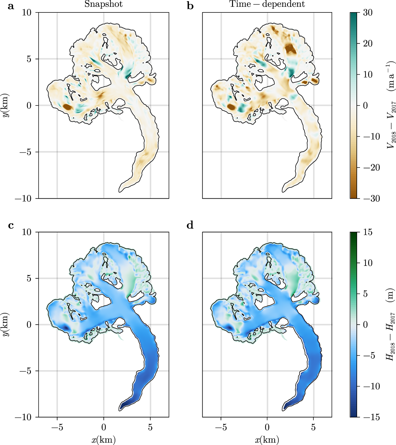
Our study lays out a broadly applicable inversion method that can be adapted to more sophisticated ice-flow models with ease; the forward model could be replaced with a different physical ice-flow model or even a machine learning model, such as a neural net. This flexibility is possible as the employed AD tool (Enzyme used within Julia) can differentiate through almost arbitrary Julia code, including physical and statistical models. Recent advances in machine learning have resulted in the development of promising data-driven parameterisations for surface processes, which capture spatiotemporal variations in climate and weather forcing (Anilkumar and others, Reference Anilkumar, Bharti, Chutia and Aggarwal2023; van der Meer and others, Reference van der Meer, Zekollari, Huss, Bolibar, Sjursen and Farinotti2024). Using AD would enable efficient fine-tuning of these data-driven parameterisations to be used in combination with physics-based ice-flow models, resulting in better predictions. The versatility of our approach also extends to which fields are inverted for and could be readily adapted to target bed topography and/or SMB instead of only reconstructing the basal sliding coefficient. This versatility is made possible by the use of AD and GPU acceleration, allowing for efficient and robust optimisation procedures.
We aim to enable predictive modelling at regional and global scales, utilising the ever growing spatial and temporal resolution of observational data. Physics-based forward models capture a broad range of physical processes but demand substantial computational resources at target resolution. Overcoming this challenge necessitates the use of modern supercomputers, which are predominantly powered by GPUs. It is thus essential to develop models with GPU optimisation in mind. The Julia programming language uniquely combines high-level functionality with native support for GPUs and AD. This study demonstrates the integration of high-performance GPU computing and AD-powered adjoint sensitivity analysis within a high-level programming environment. Implemented entirely in Julia, the codebase enhances reproducibility and accessibility, making it both efficient and educationally valuable. Unlike traditional implementations in low-level languages, this approach streamlines development and reduces complexity, enabling faster, more accessible model refinement.
The performance benchmark for the forward SIA solver demonstrates that GPU acceleration dramatically reduces time-to-solution for the forward model. With speedups beyond two orders of magnitude compared to a CPU code, the GPU-accelerated code significantly shortens the runtime of the forward solver, making larger-scale inversions feasible. Such inversion workflows often require the forward solver to be executed numerous times, underscoring the importance of this performance gain. The substantial bandwidth provided by GPUs, when effectively utilised, accelerates computations in such memory-bound computations.
In this study, we included only two time points in the time-dependent inversion, made possible by employing implicit time integration of the forward model. This approach eliminates the need to store intermediate results for reverse-mode AD evaluation. In contrast, the often-used explicit time integration in glaciological forward models requires numerous time steps and, thus, would require complicated checkpointing schemes for practical inversions to limit memory requirements during reverse-mode AD (see Section 2.4). Given the typical temporal sparsity of many glaciological datasets and the efficiency of implicit time stepping for ice-flow simulations (Bueler, Reference Bueler2023), our approach, using implicit time integration with larger time steps combined with the adjoint state method, reduces the need for slow and complex checkpointing algorithms, which trade storage for redundant forward model computations and thus can be a significant computational bottleneck (Stumm and Walther, Reference Stumm and Walther2010).
Previous studies have demonstrated that AD-based inversions, including both snapshot and, more recently, time-dependent approaches, are feasible and yield useful results (e.g. Goldberg and Heimbach, Reference Goldberg and Heimbach2013; Larour and others, Reference Larour2014; Goldberg and others, Reference Goldberg, Heimbach, Joughin and Smith2015). However, the computational demands associated with these methods remain a significant challenge (Choi and others, Reference Choi, Seroussi, Morlighem, Schlegel and Gardner2023).
This study demonstrates that such inversions can be effectively performed on GPUs with good performance, suggesting that this approach could enable broader adoption of these methods in the future. An alternative approach to achieve potentially even higher performance involves the use of statistical emulators (e.g. Brinkerhoff and others, Reference Brinkerhoff, Aschwanden and Fahnestock2021; Jouvet, Reference Jouvet2023). However, this comes at the cost of reduced fidelity or the risk of failure when applied outside the domain spanned by the training data.
The method employed in this study is similar to other adjoint-based, time-dependent inversions. However, the solver used—the APT method—is a matrix-free approach particularly well suited to GPUs, as it requires very few global operations, which are typically the primary bottlenecks in GPU computations.
Replacing the SIA forward model with a depth-integrated higher-order model, such as DIVA or L1L2 (Schoof and Hindmarsh, Reference Schoof and Hindmarsh2010; Goldberg, Reference Goldberg2011; Robinson and others, Reference Robinson, Goldberg and Lipscomb2022), should improve the accuracy of parameter reconstructions and enable inversions in regions where membrane stresses are significant, such as dynamic areas of ice sheets or faster-flowing alpine glaciers. Adapting the code to support these higher-order models is feasible, as the current design already solves nonlinear elliptic equations and their corresponding linear adjoint state equations, which are required for such models. Although this modification will increase the computational cost of the model evaluations, it remains feasible due to the GPU-based implementation. For context, one of the presented Aletsch inversions takes a few minutes on a single Nvidia A100 GPU, demonstrating that even more computationally expensive model runs could be handled.
Our study supports the findings of, e.g., Goldberg and Heimbach (Reference Goldberg and Heimbach2013); Larour and others (Reference Larour2014); Goldberg and others (Reference Goldberg, Heimbach, Joughin and Smith2015); Choi and others (Reference Choi, Seroussi, Morlighem, Schlegel and Gardner2023) that time-dependent approaches can accurately reconstruct basal properties of glaciers. This type of inversion is particularly valuable for studying systems that are inherently time-dependent, such as the ice geometry evolution investigated in this study, or subglacial hydrology and its relationship to ice dynamics. In alpine environments, these advanced inversion methods could provide insights into the evolution of glacier sliding, for instance, improving our understanding of hazards linked to sliding instabilities of steep glacier tongues (Faillettaz and others, Reference Faillettaz, Sornette and Funk2010).
5. Conclusion
The main contribution of this work is the development of a method and numerical implementation to reconstruct a spatially variable glacier basal sliding coefficient using automatic generation of adjoint code via AD on GPUs. Our main findings highlight that (i) combining both geometry change and velocity in the objective function provides a more accurate reconstruction of the sliding parameter; (ii) time-dependent inversion provides a better quality fit of the basal sliding parameter improving surface velocity reconstruction compared to the snapshot inversion; and (iii) working with higher spatial resolution improves the inversion quality on the Aletsch glacier, with converging results for spatial resolutions between 50 and 25 m, close to that of the observational dataset. Given the computational expense of running time-dependent inversions on high-resolution data, leveraging new tools such as GPU processing and automatic generation of adjoint code using AD is essential. These advancements are crucial for advancing time-dependent inversions to a new level, both in spatial and temporal resolution.
Acknowledgements
We thank Guillaume Jouvet and Daniel Farinotti for discussions on time-dependent versus snapshot inversions that helped shape the study. Computations were performed on an Nvidia 8 x A100 GPU server acquired through an ETH Zurich equipment grant. This work was supported by the Platform for Advanced Scientific Computing (PASC) project ‘GPU4GEO’ and by a grant from the Swiss National Supercomputing Centre (CSCS) under project ID c23.
We provide the exact version of the Julia Glacier slide software Glaide.jl needed to reproduce the figures and results of this paper as an archive on Zenodo https://doi.org/10.5281/zenodo.13793630 (Utkin and others, Reference Utkin, Chen, Räss and Werder2025). Present and future releases of Glaide.jl can be found on GitHub at https://github.com/yiluchen1066/Glaide.jl. As some of the data cannot be retrieved in an automated fashion from within the data generation notebook (Utkin and others, Reference Utkin, Chen, Räss and Werder2025), we provide them from a persistent data repository (Utkin and others, Reference Utkin, Räss, Werder and Chen2024).
Author contributions
IU and LR designed the study which was at first developed during the Master Thesis of YC. IU developed the mathematical and numerical formulations. YC and IU coded the numerical implementation. All authors contributed to data visualisation and paper writing. Artificial intelligence tools were used only for improving text at the sentence level and for boilerplate code generation.
Competing interests
The authors declare that they have no conflict of interest.


 Open access