1. Introduction
Polarisation studies in VLBI are a delicate probe of the internal conditions of the radiating material, as the polarisation fraction and direction are directly related to the magnetic field in the emission region. Polarised VLBI studies have important contributions to make, for instance, in star-forming regions and AGN environments.
Therefore the Australian Long Baseline Array (LBA), with its near exclusive view on the Southern sky, has the potential to carry out a major polarisation research effort. This would take advantage of the large collecting area, which is larger than that of the VLBA (even though the number of stations is only half). However, polarisation studies with the LBA are few and far between. Until 2008, the nonstandard mount type at the Hobart telescope meant that the longer baselines in the LBA could not be calibrated, and the triangle between Parkes, Mopra, and Australian Telescope Compact Array (ATCA) had only short-baselines (∼200 km) with very similar feed angles, making it hard to disentangle the instrumental feed contributions (the D-terms) from the polarised sky signals. Nevertheless, one paper did produce preliminary images of G340.054−0.244 (Bains et al. Reference Bains, Caswell, Richards, Phillips, Tingay, Kramer, Cohen, Cunningham, Chapman and Baan2007). After the Hobart E-W mount type was included in AIPS (Greisen Reference Greisen2003) polarisation calibration was possible; the increase in the number of antennas with the commissioning of Ceduna also helped. This was demonstrated in a number of technical reports (Dodson Reference Dodson2007, Reference Dodson2009) and in Dodson (Reference Dodson2008) which present a study on the high resolution polarisation structure in Methanol masers. In addition, Dodson & Tzioumis (Reference Dodson and Tzioumis2013) describe how the contemporaneous ATCA data can be used to provide the absolute polarisation angle for LBA calibration.
Shortly after the Astronomical Image Processing System (AIPS) had been updated to cope with E-W mounts, ATCA underwent a major upgrade that increased the bandwidth from 128 MHz to 2 GHz (Wilson et al. Reference Wilson2011). A downside of this was that: (i) the VLBI mode was given a low priority for several years, (ii) the delay calibration became much more complex, as now it had to be valid for a much larger frequency range, and (iii) the residual delays leaked into the system that forms the tied-array output from the individual linear inputs. The consequence of this was that ATCA in VLBI mode was, compared to previously, poorly calibrated and unstable for polarisation observations. While poor calibration can be fixed (by calculation of the D-term correction), time-varying D-terms are hard to measure and AIPS has no simple means for applying such a correction.
However, polarisation VLBI continues to be an important capability for any array. Therefore we have undertaken a major effort to track down and overcome all these complicating problems. This report presents the outcomes of this effort. That is a demonstration that now the LBA has a robust polarised performance, can be corrected for instrumental polarisation, and that these solutions are stable. Furthermore, for cases where the instrumental polarisation errors are unacceptably large, we have investigated using the post-correlation conversion from linear polarisations to circular polarisations, and using the nonlinear elliptical solutions inside AIPS. The former allows the recording of linear signals for accurate conversion in post-processing, and the latter would use nonlinear solutions to address the large D-terms. These tests are to discover the best strategy to increase the accuracy of future VLBI polarisation observations with the LBA.
It should be noted that all the LBA feeds at these frequencies detect linear polarisation from the sky; these are then converted to circular polarisation by forming the correctly phased sum of the linears. For all the single dishes except Parkes (at these frequencies) these are done with analogue hybrids, for which it is important that the input signals are equalised in gain and delay. At the ATCA the linear signals from each antenna are digitised and can be combined to form a summed circular after array calibration. Alternatively ATCA can provide a summed linear signal. These signals can then be recorded on the VLBI system.
2. Observations
We carried out two sets of observations on 2016 October 18 and 2017 March 17 (obs. code VT23A and B) to investigate the polarisation calibration strategies, summarised in Table 1. Both were observed using the Australian VLBI antennas ATCA (At), Ceduna (Cd), Hobart (Ho), Mopra (Mp), and Parkes (Pa) as part of the LBA. At, Mp, and Pa are run by CSIRO and are located in NSW on the east coast of Australia. Ho and Cd are run by the University of Tasmania and are in Tasmania and South Australia, respectively. The parameters of all five antennas are shown in Table 2.
General information on the experiments VT23A and VT23B. Note that Project VT23B contains two data sets: (1) the circular data, where all antennas recorded the nominally circular polarisation and (2) the mixed data, where At directly recorded its linear polarisation.

Observational parameters of the five LBA telescopes.
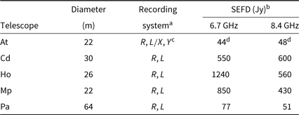
a R, L and X, Y represent nominally circular and linear polarisation recording, respectively.
b The System Equivalent Flux Density (SEFD) of 6.7-GHz bands (from http://www.atnf.csiro.au/vlbi/documentation/vlbi_antennas/index.html, updated for the new CX-band feeds on At and Pa).
c For VT23B ATCA recorded both circular and linear polarisations, for the same frequency setup.
d The combined SEFD of five antennas.
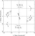
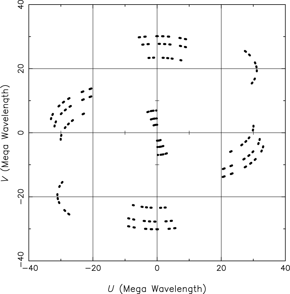
The baseline lengths range from ∼100 km (At to Mp) to ∼1 700 km (Ho to Cd), providing good sensitivity to both compact and more extended emission. The experiment VT23A consisted of 5 h of observations with a bandwidth of 64 MHz in nominal Left- and Right-Hand Circular Polarisation (LCP and RCP, respectively) at 8 393 MHz. VT23B consisted of 7 h of observations with a two contiguous bandwidths of 16 MHz each (upper and lower sideband) at 6 658 MHz. For this experiment ATCA simultaneously recorded two sets of data at the same frequency. The outcome in the first case is nominally circular polarisation data set, and in the second case it is a mixed polarisation data set, which required further post-processing. One fringe-finding source (1921−293) was observed for 10 min for bandpass and clock offset corrections. Eight compact strong sources were observed for the polarisation analysis: 0135−247, 0142−278, 0234−301, 0227−369, 0146+056, 0237+040, 0426−380, and 0451−282, summarised in Table 3. The last four sources were observed only in VT23B. Scans of approximately 6 min in length of the targets were arranged in cycles to maximise the UV-coverage which produces sampled visibility function and minimise the slew times. This gave about 50–70 min of observing time per source and an expected sensitivity of 60–70 μJy/beam. The UV-coverage of the target source 0135−247 from the experiment VT23B is shown in Figure 1 for an example showing sufficient UV-coverage from short and long baselines. The data were correlated using DiFX (Deller et al. 2011), with 256 and 64 channels across the band for VT23A and VT23B, respectively, allowing delays up to 100 ns to be corrected for without significant loss. All four Stokes products were correlated. VT23B was correlated twice, once with At circular data and once with At linear polarisation data.
The typical UV-coverage of the AGN target sources from the experiments, for 0135-247 in VT23B.
General information for eight AGN target sources observed in this work.

b Peak flux density from X band images.
3. Methodology
Polarisation calibration is a well-established part of VLBI analysis (e.g., Kemball, Diamond, & Cotton Reference Kemball, Diamond and Cotton1995). We present here how we undertake the calibration for the LBA data sets, underlining aspects of particular importance and special considerations for the Australian array.
Initial calibration: Initial data reduction was done following the standard procedures in AIPS with tasks: ACCOR corrections to the autocorrelations, CLCOR to update the Earth Orientation Parameters and to correct for the feed rotations, and TECOR to correct for the ionospheric propagation effects. The first calibration step after this is to apply the system temperatures for the antennas, derived from the experimental logs. This information is to be found on the experiment website, hosted by the Australia Telescope National Facility (ATNF). For Ho and Cd, the University of Tasmania extracts this information from the Field SystemFootnote a logs, and these are usually all that is required, for these antennas. The ATNF antennas instead can extract system temperature information from the ATNF logging, but in truth often-times one is forced to use the tabulated canonical values. These values are best collated into a text file and attached to the database via ANTAB. Once the antenna system temperatures and gain values are attached, we usually apply them via the AIPS scripts within the VLBAUTIL RUN file: VLBACALA, VLBAEOPS, VLBATECR, and VLBAPANG, although if the user is comfortable with manually running through the steps this should be no issue (all procedures of each script are described in Appendix A). Next, phase and amplitude variations as a function of frequency of our prime calibrator, 1921−293, were corrected using BPASS. Amplitude corrections from the system temperatures were significantly more complicated as the system temperature and efficiency measurements were incomplete. Therefore we scaled the observations of the prime calibrator to be 7.919 and 7.773 Jy at 8.4 and 6.7 GHz, respectively (the catalogued flux values observed at ATCA close to our observation datesFootnote b), using SETJY and CALIB. After this initial amplitude calibration we could self-calibrate the data for residual phases, rates, and delays, using FRING.
Self-calibration on Stokes I images: Afterwards, the sources in the single UV-data file were frequency averaged over each IF into separate files. Each single source file was used for imaging in Difmap [the interactive editing and mapping software (Shepherd Reference Shepherd, Hunt and Payne1997)]. However, users can use AIPS or other softwares for mapping, depending on one’s preference. The imaging process is mainly based on phase and amplitude self-calibration and CLEAN, and only Stokes I is considered. After achieving high-quality images (having the best possible SNR), we recalibrated the data in AIPS, using the difmap source models and CALIB, to provide the phase and amplitude self-calibration tables in AIPS, with the solution intervals of 2 and 30 min, respectively. This is a vital stage, particularly for the LBA, as if the amplitudes for the input data are not accurately calibrated the derived D-terms will be contaminated. We would recommend, if feasible, including regular scans of a strong maser line in the observations to provide an independent measure of the system equivalent flux density, to be derived with ACFIT.
Polarisation calibration: Cross-polarisation delays for the right- and left-handed data for all baselines were corrected by applying the VLBACPOL script to data for a scan showing a clear polarisation signal for all baselines to our reference antenna.
To determine the effective feed parameters (D-terms) of LBA antennas from the calibrated visibility data, we firstly used LPCAL task, based on the assumption of linear approximation for the feed response. After solving for the feed’s polarisation corrections, SPLIT task was used to apply the polarisation corrections to all antennas to retrieve the corrected values.
Additionally, as Mopra often has large D-terms, of the order of 10%–30%, an alternative solution for Mopra would be to record the linear polarisations and convert to circular post-correlation. This would replace the normal practice for linear polarisation antennas, such as Mopra, of converting to circular polarisation pre-correlation. To test this we used an updated version of PolConvert (Martí-Vidal et al. Reference Martí-Vidal, Roy, Conway and Zensus2016), which solves for the delays between R and L at the reference antenna, as well as correcting the mixed linear-circular correlated data, post-correlation. At ATCA we observed both linear and circular polarisations at the same frequency using the two frequency-channel setups and two on-site VLBI recorders. In one case, the linear polarisations were calibrated during setup and combined in the tied-array controller to produce a circular output for the VLBI recorder. Simultaneous observations with the same setup, but without the conversion from linear to circular, were recorded in parallel. The PolConvert correction process is very simple, being presented as a task within CASA (McMullin et al. Reference McMullin, Waters, Schiebel, Young, Golap, Shaw, Hill and Bell2007) that reads the DiFX output. After correcting the data, the updated file is read into AIPS for a standard processing. The same steps were followed for both the nominally and mixed-corrected circular polarisation data, and LPCAL task was used to solve for D-terms.
Furthermore, AIPS also supports nonlinear D-terms, which we suspected could be important for antennas with poor initial polarisation purity (i.e., beyond the linear regime). However, this functionality is only available via the compact array polarisation task, PCAL. Therefore we also investigated this option, which allows for elliptical polarisation D-terms. PCAL is not recommended for VLBI, as it does not cope well with resolved sources. However, all our targets are compact in VT23A, making this comparison possible.
Firstly, we confirmed that PCAL returns the same linear solutions as LPCAL by comparing the results for the PCAL using the ‘resolving linear approximation’ option to those from LPCAL, which is designed for highly resolved sources, but only support the linear approximate option. Secondly, we compared the residual RL/RR and LR/LL, for baselines with Mp, for the PCAL elliptical and LPCAL linear D-terms.
Polarisation imaging: Finally, we used Difmap to create the polarisation maps (linear polarisation vectors and angles spatially overlaid on Stokes I contours) from corrected UV-data files. To obtain high-quality polarisation images, all Stokes (I, Q, U, V) should be carefully mapped, as the linear polarisation fraction and angle are sensitive to the intensities of Stokes parameters (the relations are described in Appendix B).
The aim of this experiment was to demonstrate that polarisation calibration could be performed with the LBA. The design was to allow comparison of different polarisation methods and compare the results between sources and IFs where possible. Therefore, the schedule did not include an absolute polarisation calibrator. Nevertheless, following Dodson & Tzioumis (Reference Dodson and Tzioumis2013), we have investigated using the absolute position angle (PA) on arcsecond-scales for one of the compact sources (0142−278) using the contemporary ATCA data. However none of our ATCA observations produced significant polarisation measurements and this approach could not be applied. The sensitivity of ATCA compared to the LBA is less because of the smaller total collecting area of the array and the larger beam dilution effect, whilst the bandwidth remains the same.
4. Results
4.1. Linear model (LPCAL)
4.1.1. Nominally circular polarisation
All AGN calibrator sources observed in VT23A and B were calibrated as described in Section 3 providing the RCP and LCP D-terms for all antennas as shown in Figures 2 and 3 and summarised in the first three columns of Table 4. Figure 2 and 3 show the fractional RCP and LCP D-terms on the complex plane for all five antennas (At, Cd, Ho, Mp, and Pa) from experiment VT23A (8.4 GHz) and VT23B (6.7 GHz), respectively. Each shows the results from all the AGN calibrator sources in the experiment: the averaged absolute D-terms and the standard deviation between the sources (listed in Table 4). For VT23B the D-terms for two IFs were solved for independently, whilst for VT23A there was only one IF. For each antenna and each circularly polarised feed (RCP or LCP), the measured D-terms are quite stable between calibrators, with very small uncertainties of ∼1%, as listed in Table 4. For experiment VT23A (the first column), where additional effort was made at the observatories to ensure polarisation purity, At and Pa are nearly perfect for both RCP and LCP feeds with small D-terms of ∼1%. Cd has one good polarisation and one poor, with LCP D-term of ∼1% whilst that of RCP is ∼7%. Mp has the largest D-terms of ∼17% and ∼13% for RCP and LCP feeds, respectively, and Ho shows fairly high D-terms of ∼8% for both RCP and LCP feeds.
Absolute percentage Values for the D-terms from LPCAL and the Standard Deviation over the eight targets, from the Pure circular polarisation (both VT23A and VT23B) and the Linear mixed polarisation after post-correlation conversion to all circular (only VT23B). Solutions are from LPCAL; the UV data were preaveraged to 0.3 and 0.7 min (SOLINT) for VT23A and VT23B, respectively, and the Stokes I target image was used as an input and limited to a single polarised component.
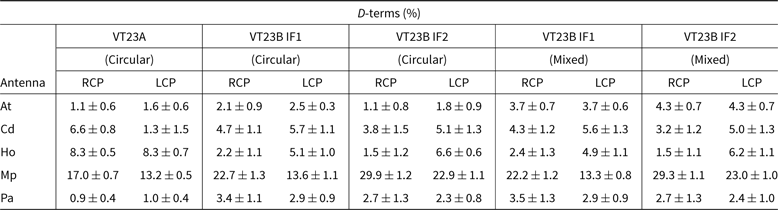
For experiment VT23B (the second and third columns) Mp has significantly worse performance, with higher D-terms, than in VT23A and shows significant differences between the two IFs as shown in Figure 3, whilst all other antennas have acceptable D-terms, with a mean value of ∼3%.
D-terms measured with LPCAL, for all the antennas in VT23A, At (red), Cd (green), Ho (blue), Mp (cyan), and Pa (black), at 8.4 GHz. For a given antenna, DR values from observations of individual sources are shown with solid lines and for DL with dot-dashed lines. Note the very small scatter between sources (enclosed within the larger circle), the accurate initial instrumental polarisation for At, Cd, and Pa (with a few per cent), larger values for Ho, and very large D-term values for Mp. In all cases, the values from individual sources are consistent at a similar level.
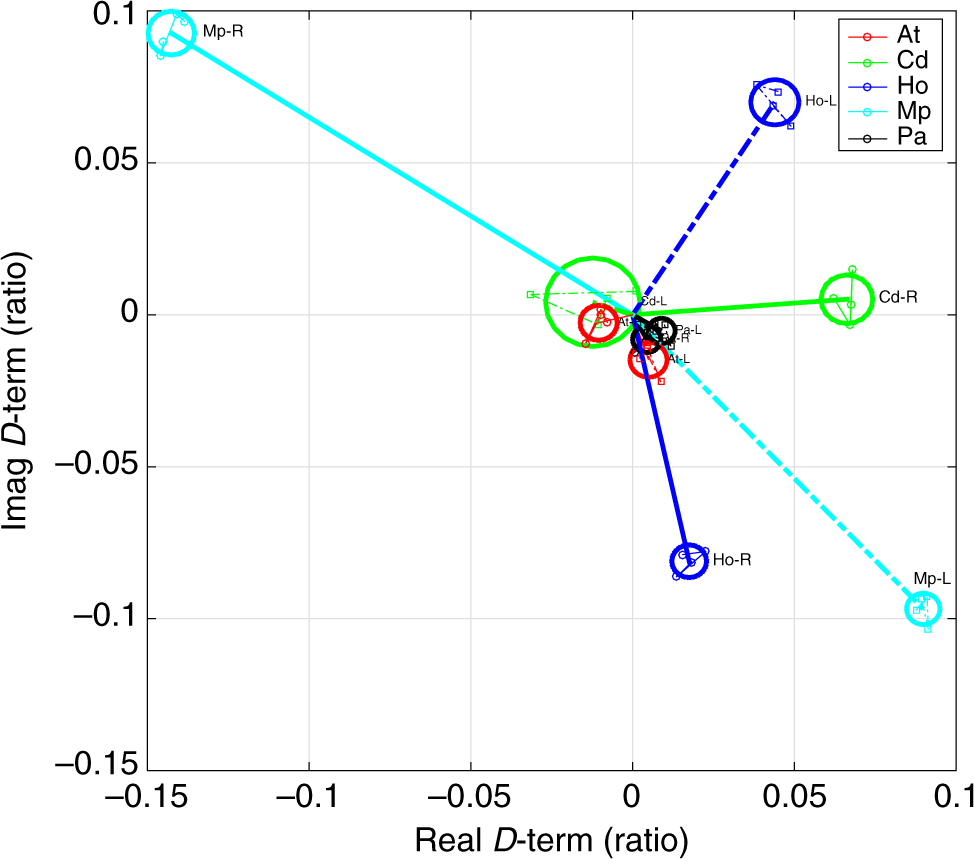
D-terms measured with LPCAL, for all the antennas in VT23B, with two independent IFs at 6.642 (a) and 6.658 (b) GHz, for each of the eight targets, for all of the antennas. See Figure 2 for the description of the symbols. Note the reasonable agreement between IFs for At, Cd, Ho, and Pa but quite different terms for Mp.
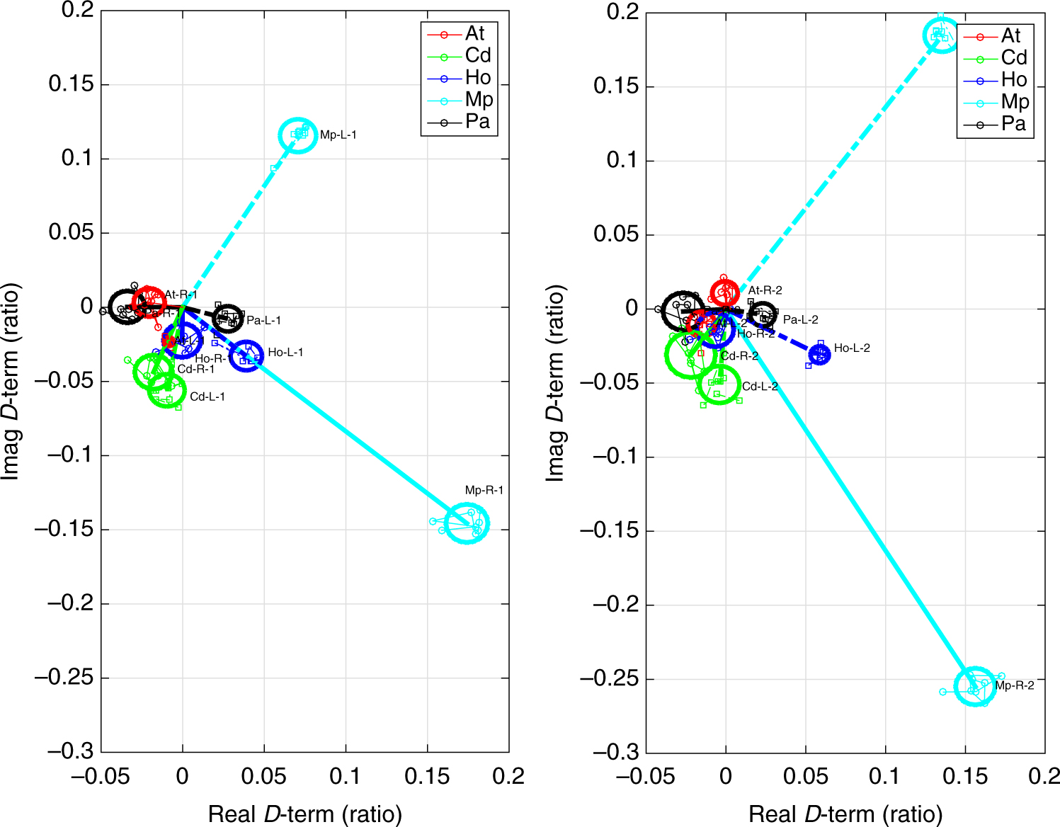
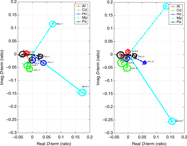
Figure 4 shows examples of LR/RR plot from the Mp baseline to At, Cd, and Ho, for the source 0135−247 from the experiment VT23A in the complex plane before and after polarisation calibration using LPCAL. This shows that before calibration the data values are circularly distributed around an origin, whilst after calibration all the data lies at the centre, thus demonstrating that the instrumental D-terms have been properly corrected.
Correlated RL/RR of 0135-247 on the complex plane before (left) and after (right) polarisation calibration from Mp baselines. The collapses of the circular distributed values determine the quality of the polarisation solutions; the residual standard deviations of the correlated RL/RR after polarisation calibration are mentioned at the upper-right corners. (a) Before polarisation calibration (At−Mp). (b) After polarisation calibration (At−Mp). (c) Before polarisation calibration (Cd−Mp). (d) After polarisation calibration (Cd−Mp). (e) Before polarisation calibration (Ho−Mp). (f) After polarisation calibration (Ho−Mp). (g) Before polarisation calibration (Mp−Pa). (h) After polarisation calibration (Mp−Pa).

4.1.2. Mixed polarisation (use of PolConvert)
The last two columns of Table 4 show the D-terms of all antennas from project VT23B where ATCA recorded linear polarisation, whilst all other antennas still recorded in circular polarisation. The At data were then calibrated and converted to circular using PolConvert on source 1921−293, post-correlation. It is shown that the D-terms of At are slightly increased to ∼4% for both RCP and LCP and both IFs; however, the D-terms of the other antennas, considering their uncertainties, are identical with those from the nominally circular polarisation data, as expected.
4.2. Ellipticity-Orientation model (PCAL)
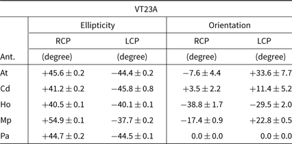
In addition to the Linear model from LPCAL, for the experiment VT23A we also used the Ellipticity-Orientation model in PCAL task to determine and correct the polarisation-induced instrumental errors and compare the solutions with LPCAL task, particularly for Mp baselines. For this task, the solution type ORI− was selected. In this case the Pa telescope is very close to ideal, so it was used as a reference antenna. With this model the instrumental imperfections are parameterised by two parameters: ellipticity and orientation. These two parameters, derived for all antennas, are listed in Table 5. For a perfect circular feed, the ellipticity of RCP and LCP feeds should be close to +45° and −45°, respectively, based on the definition used in AIPS, and the orientation should be undefined or equal to zero. The deviation from those values will introduce some level of false linear polarisation fraction and angle. Considering the instrumental induced linear polarisation fraction from ellipticity, At and Pa are close to perfect with the deviation less than 1°, corresponding to their small D-terms. The RCP and LCP feeds of Cd are poor (∼4° error) and good (less than 1°), respectively, which are in good agreement with their D-terms. The largest deviations of ∼10° and ∼7° are found from RCP and LCP feeds of Mp, respectively; Ho shows fairly high deviations of ∼5°.
The ellipticities and orientations of RCP and LCP feeds of each antenna for the experiment VT23A from PCAL with solution type (SOLTYPE) ORI−; the other input parameters were the same as in LPCAL task.
4.3. 8.4 and 6.7-GHz polarisation maps and polarisation fractions
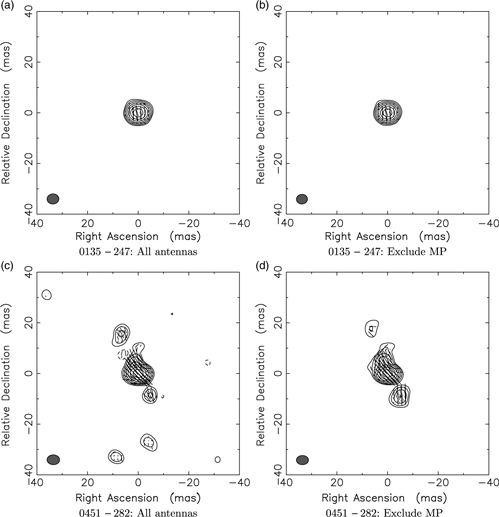
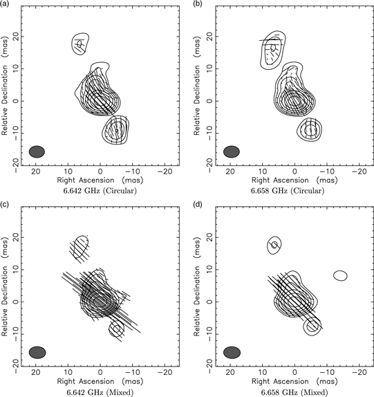
We created the polarisation images of all AGN sources from the experiment VT23A and VT23B (both Circular and Mixed data) to derive the polarisation fractions at the Stokes I peak positions which are listed in Table 6. We made two separate sets of the polarisation maps, with and without Mp, to test whether the image quality can be further improved by excluding the worst antenna. We found a trend of slight decrease and increase in dynamic range (DR) for VT23A and VT23B, respectively, after flagging Mp, without impacting polarisation fractions. More than half of the target sources (five out of eight) are of good image quality with and without Mp, whilst the others (i.e., 0146+056, 0237+040, and 0451−282) show poorer image quality with the inclusion of Mp as illustrated by examples in Figure 5(a) and (b) for the source 0135−247 and (c) and (d) for the source 0451−282, respectively.
Comparison of Stokes I peak flux (the third column), Stoke I image noise (the fourth column), image dynamic range (the fifth column), polarisation flux at the Stokes I peak position (the sixth column), polarisation rms noise  $\left(\sqrt[]{Q_{\rm rms}^2+U_{\rm rms}^2}\right)$ (the seventh column), linear polarisation fraction with uncertainties (the eighth column; asterisk (*) symbol marks unpolarised fractions with P/P rms < 4), and polarisation angle (measured anticlockwise from North) (the ninth column) between eight AGN sources from the experiment VT23A and VT23B excluding Mp.

The examples of 6.642-GHz polarisation maps from the experiment VT23B for 0135−247: (a) and (b), and 0451−282: (c) and (d) created with and without MP telescope, respectively. The imaging parameters used are 512 × 512 pixels with cell size of 0.5 mas. Contour levels are −1%, 1%, 2%, 4%, 8%, 16%, 32%, and 64% of the peak fluxes and linear polarisation vectors are set to 500 mas/Jy in length and plotted every three pixels where Stokes I fluxes are greater than 30 mJy. The beamsize is shown as a filled ellipse in the lower-left corner of each map. Whilst the tabulated polarisation flux and PAs with and without Mopra agree, it is clear that the image quality can be degraded.

Furthermore, we have compared the polarisation flux and PAs measured in the data formed from the two IFs, and the nominally circular polarisation data compared to the mixed polarisation data, in experiment VT23B. The latter tests the reliability of these two nominally equivalent calibration approaches, although with different primary calibrators used to set the zero point (0823−500 and 1921−293, respectively) in the data. This solution reference point will absorb all residual errors in the data at this point in the data reduction, such as the fractional polarisation and/or structure of the source and the effects from uncorrected delays. The D-term solutions in AIPS are calculated after these effects are corrected for and therefore the solutions can also be different. We find that the polarisation angles agree to about 10° and the polarisation fraction agrees within 1% between the two data sets and two IFs for all sources except for the high polarisation sources 0237+040 and 0451−282, which show significant differences in polarisation fraction between the Circular and Mixed data of 1.6% and 1.5% for IF2 and IF1, respectively. This is an evidence that we may have underestimated of our errors of 0.1%–0.2%. However, in most cases the differences are under 0.5%, which we consider to be within expectations.
It can be seen from the maps that all AGN sources are compact sources with peak flux densities greater than 500 mJy. Overall, all four AGN sources in VT23A at 8.4 GHz have very small polarisation fractions, below 1%, which increase up to ∼1% for VT23B at 6.7 GHz. The last four sources in Table 6 which were observed only at 6.7 GHz show comparatively high polarisation fractions, approximately ranging from 1% to 4%. One of these sources, 0451−282, is well resolved and of apparently extended structure. Reviews and results from polarisation images for all eight AGN sources are as follows:
PKS 0135−247 (J0137−2430): This source is a bright quasar at a red-shift of 0.8. It is included in the VLBA Calibrator Survey (Petrov et al. Reference Petrov, Kovalev, Fomalont and Gordon2008) and The Radio Fundamental CatalogFootnote c (Petrov Reference Petrov2016) reports a compact source with peak flux densities from 8.6-, 4.9-, and 2.3-GHz images of 0.3 (epoch 1999), 1.1 (epoch 1996), and 0.4 (epoch 1999) Jy with weak jets in the northeast that resolve at about 125, 70, and 50Mλ, respectively. In this study, we obtained flux densities of ∼1.2 and ∼1.4 Jy with no linear polarisation detection (∼1σ) and with linear polarisation fraction of ∼0.7% (∼6σ) on average at 8.4 and 6.7 GHz, respectively. Moreover, at 8.4 GHz, we found a slightly extended region in the northeast as illustrated in Figure 7(a) (Appendix E) supporting the weak jet structure from the Radio Fundamental Catalog; however, this structure is invisible at 6.7 GHz.
PKS 0142−278 (J0145−2733): This source is a quasar at a red-shift of 1.1. The Radio Fundamental Catalog reports a compact source with peak flux densities from the 15.4-, 8.7-, and 2.3-GHz images of 0.6 (epoch 2016), 0.3 (epoch 2015), and 0.6 (epoch 2015) Jy with weak jets in the northeast that resolve at about 80, 100, and 60Mλ, respectively. Additionally, from the MOJAVE databaseFootnote d (Lister et al. Reference Lister2009), it also shows a strong jet at 15.4 GHz and the peak flux density of 0.6 Jy and the polarisation fraction of 0.5% (epoch 2016). In addition, high variation of flux density and polarisation fraction with time are found between epoch 2009 and 2016; the highest polarisation fraction of 4.4% was detected in epoch 2013. Our study obtained peak flux densities of ∼0.8 and ∼0.7 Jy with polarisation fractions of ∼0.5% and ∼1% at 8.4 and 6.7 GHz, respectively. At 8.4 GHz, we also found significant extended polarisation structure in the east region as shown in Figure 8 (Appendix E) corresponding to the result from MOJAVE database; however, this trend is not found at 6.7 GHz.
PKS 0227−369 (J0229−3643): This source is a quasar at a red-shift of 2.1. The Radio Fundamental Catalog reports a compact source with peak flux from the 8.6- and 2.3-GHz images of 0.4 (epoch 2017) and 0.3 (epoch 2017) Jy. We found the peak flux density of ∼0.5 and ∼0.6 Jy at 8.4 and 6.7 GHz, respectively, with no polarisation fraction for both frequencies (∼2σ and 3σ on average). However, for IF2 of Mixed data at 6.7 GHz, the polarised flux is ∼6σ which, in this case, can be regarded as an underestimated σ.
PKS 0234−301 (J0236−2953): This source is a quasar at a red-shift of 2.1. The Radio Fundamental Catalog reports a compact source with peak flux from the 8.7- and 2.3-GHz images of 0.3 (epoch 2015) and 0.2 (epoch 2015) Jy, respectively. Our study obtained peak flux densities of ∼0.5 and ∼0.6 Jy with no (∼2σ) and with polarisation fraction of ∼1% (∼9σ) on average at 8.4 and 6.7 GHz, respectively. At 6.7 GHz, only IF1 of Circular data has comparatively low polarisation fraction (∼3σ), while the others show obvious polarisation detections (with a range of ∼6σ–16σ).
PKS 0146+056 (J0149+0555): This source is a quasar at a red-shift of 2.3. The Radio Fundamental Catalog reports a compact source with peak flux from the 15.3-, 7.6-, 4.3-, and 2.3-GHz images of 0.7 (epoch 1998), 0.4 (epoch 2016), 0.6 (epoch 2016), and 1.1 (epoch 2016) Jy, respectively. At 15.3 and 7.6 GHz, powerful jets are detected in the east, whilst at 4.3 GHz, there are weak jets towards the south and the southwest; those resolve at about 100Mλ. We obtain peak flux densities of ∼1.2 Jy and average polarisation fractions of ∼1% (∼10σ) at 6.7 GHz; however, no extended structure is detected in our study as illustrated in Figure 11 similar to the 2.3-GHz image of the Radio Fundamental Catalog.
PKS 0237+040 (J0239+0416): This source is a quasar at a red-shift of 1.0. The Radio Fundamental Catalog reports a compact source with peak flux from the 7.6-, 4.3-, and 2.3-GHz images of 0.2 (epoch 2018), 0.4 (epoch 2018), and 0.6 (epoch 2013) Jy, respectively, with fairly strong jets in the northwest that resolve at about 150Mλ at 7.6 and 4.3 GHz and a weak jet in the same direction at 2.3 GHz that resolve at about 70Mλ. We found peak flux densities of ∼0.6 Jy and a high polarisation fraction of ∼3% (∼20σ) on average at 6.7 GHz.
PKS 0426−380 (J0428−3756): This source is a bright quasar at a red-shift of 1.1. The Radio Fundamental Catalog reports a compact source with peak flux from the 8.6-, 4.9-, and 2.3-GHz images of 0.4 (epoch 2000), 1.7 (epoch 1996), and 0.6 (epoch 2000) Jy, respectively; the weak jet is found only from the 4.9-GHz image in the east that resolves at about 150Mλ. We obtained the very strong peak flux density of ∼5 Jy with average polarisation fractions of ∼2% (∼28σ) at 6.7 GHz without any detected jet as shown in Figure 13 (Appendix E).
PKS 0451−282 (J0453−2078): This source is a bright quasar at a redshift of 2.6. It is included in the VLBA Calibrator Survey. The Radio Fundamental Catalog reports very elongated structure at 15.4-, 8.6-, 4.3-, and 2.3-GHz images implying the strong jet in the north with flux density of 1.1 (epoch 2013), 1.2 (epoch 2016), 1.2 (epoch 2016), and 1.2 (epoch 2016) Jy that resolves at about 400, 350, 100, and 90Mλ. All bands show very strong jets in the north. The MOJAVE database also shows a similar structure for 15.4-GHz image with peak flux density of 1.1 Jy and strong polarisation fraction of 2.3% (epoch 2013) slightly varying with time between epochs 2009 and 2013. We obtained the peak flux density of ∼2 Jy with average polarisation fraction of ∼2% (∼17σ) at 6.7 GHz. In addition, for all the data sets, our study found the same trend of elongated structure as those from the Radio Fundamental Catalog and MOJAVE database as shown in Figure 14 (Appendix E).
5. Discussion
5.1. Linear model (LPCAL)
In this section, we used compact AGN sources (most of which are weakly polarised sources) to solve for the D-terms of five LBA telescopes using LPCAL task in AIPS, based on linear approximation (see Appendix C).
The D-terms and polarisation correction: To check the quality of polarisation solution before and after the D-term corrections, one option is to make a plot of any flux ratio in Equation (C9) (Appendix C) in the complex plane. Figure 4 shows the RL/RR ratio plots of the AGN source 0135−247 from Mp baselines before and after polarisation correction. The other cross to parallel ratios can also be used for checking in the same manner. If the instrumental D-terms have been properly corrected, all data values should shrink towards the origin as shown in Figure 4(b) and (h) for At–Mp and Mp–Pa baselines, respectively, (combination of large and small D-term baselines) leaving the residual standard deviations of the RL/RR ratio <1%, after which (theoretically) only the source polarisation term (p) remains. However, there remains some greater scatter for Cd–Mp and Ho–Mp baselines as shown in Figure 4(d) and (f) (combination of large and moderate D-term baselines) leaving the residuals of ∼3% and 2%, respectively, which are still able to introduce some levels of polarisation contamination.
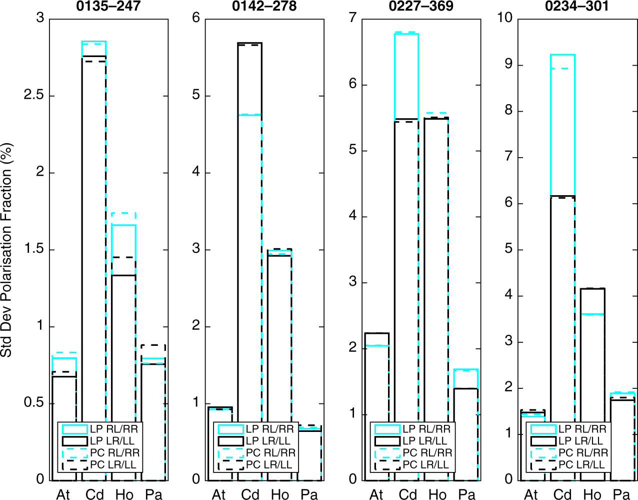
Note that the LPCAL task is based on a linear approximation of the exact expression as shown in Equation (C8) (Appendix C). As a result, the errors of the solved D-terms depend on how large the instrumental D-terms and how strong the polarisation fractions of the target sources are. Theoretically, for unpolarised sources, Equation (C8) still provides the exact D-term solutions comparable to Equation (C7) (Appendix C) even for large D-terms, but it cannot be used to correct LL and RR data because of the ignored terms. From the stable D-terms of all LBA telescopes (with small standard deviations of ∼1%), we expected that this method should work very well on solving and correcting D-terms for all antennas, even for Mp, for unpolarised or weakly polarised sources. In order to test this assumption, we calculate both RL/RR and LR/LL ratios after polarisation calibration using LPCAL task (representing the residual polarisation fraction) for four weakly polarised AGN sources from the experiment VT23A. However, we still found the same trend for all four AGN sources; i.e., that the residuals from Mp baselines are significantly larger than those for the other baselines (At–Pa, for an example, is less than ∼1%); the highest values are from large D-term baselines, i.e., Mp−Cd and Mp−Ho, and are up to ∼5% on average as illustrated in Figure 6.
Comparison of the standard deviations in the post-calibration residual polarisation fractions (RL/RR and LR/LL) for baseline visibilities from Mopra to the other antennas (At, Cd, Ho, and Pa), for all sources in VT23A. Solid lines and dashed lines are for calibration with LPCAL and PCAL, respectively. Cyan and black are for RL/RR and LR/LL fractions, respectively. There are significant non-zero values and differences between RL/RR and LR/LL, especially for Mp and Cd baselines. This indicates that the solutions for Mopra are poor. However, no significant differences can be seen between PCAL and LPCAL, showing that PCAL does not resolve the issues from the large Mopra D-terms.
The different D-terms for Mp in VT23B between IF1 and IF2 as shown in Figure 3 and Table 7 indicate the cause that these corrections change rapidly with frequency, limiting the effectiveness of a single solution per IF. Therefore, in cases where this issue is significant, one could simply exclude the Mp baselines or attempt to solve for D-terms in smaller frequency windows (see 5.3).
Absolute percentage values for four 8-MHz bandwidth D-terms (split from two 16-MHz IFs) from LPCAL and the standard deviation over the eight targets, from the pure circular polarisation of the experiment VT23B.

Table 6 lists the polarisation fractions of all sources from experiments VT23A and VT23B. The level of the fractional polarisation errors show that the LPCAL task can be applied to the LBA observations on very weak polarised AGN sources with polarisation fractions as low as ∼0.1%–0.2%, which can therefore be regarded as the residual polarisation fraction of LBA. In the case of strongly polarised sources, the residual instrumental polarisation fraction after polarisation correction is expected to be higher for baselines with large D-term antennas, in particular for Mp baselines. However, we believe LPCAL will still be suitable for strongly polarised sources, when limited to the small D-term baselines.
Use of PolConvert with the LBA: Simultaneous linear polarisation (X/Y) and circular polarisation (R/L) voltages were recorded at At, while other antennas observed in circular polarisation (R/L) only. Therefore, we could compare normal operations with that of observing with mixed polarisations, followed by conversion to pure circular polarisation using PolConvert (Martí-Vidal et al. Reference Martí-Vidal, Roy, Conway and Zensus2016). The correction was successful, with the previously linear polarisation antenna (At) now providing a near-perfect circular response. After the conversion, we applied the same calibration procedures as for the nominally R/L data. The D-term solutions for the PolConvert data were very stable between targets and robust against choosing different LPCAL settings (such as selecting the Stokes I model or assuming a point source, including or leaving out Mopra). The D-terms of At are slightly larger than those from nominally circular data; we believe this is entirely caused by the change in the reference source. In the first the polarisation calibration was during array configuration with 0823−500, and in the second the data were self-calibrated against 1921−238. The D-terms of the other antennas are the same for the two data sets; that is, this method still provides the similar residual polarisation results after correction. As a result, the Linear mixed method could be an alternative approach for LBA users. It will be very interesting to confirm whether the D-terms of Mp will be close to ideal if we recorded in linear polarisation and converted to circular post-correlation.
5.2. Ellipticity-Orientation model (PCAL)
We have also tested the PCAL task in AIPS, based on Ellipticity-Orientation model (see Appendix D), for its capability to solve the problem from the large D-term Mp.
Our PCAL results for the ellipticity and orientation of all antenna feeds derived using weakly polarised sources from the experiment VT23A are listed in Table 5. We found the corresponding trend between the D-terms from LPCAL and the deviations of the ellipticity from the perfect circular feeds for all antennas, showing the conceptual equivalence between these two models.
To test whether PCAL could be used with LBA data to correct for the highly elliptical polarisation of Mopra, we firstly confirmed that the resolving approximation solutions from PCAL based on Ellipticity-Orientation model were compatible with the results from LPCAL, based on Linear model. Then to compare the results from the two calibration tasks, we examined the standard deviation for the cross-hand to parallel-hand ratios (RL/RR and LR/LL) of the visibilities in the four AGN sources from the experiment VT23A, after polarisation calibration using the two different models. As illustrated in Figure 6, there are significant differences between RL/RR and LR/LL, especially for Mp and Cd baselines; however, the results from PCAL and LPCAL are virtually identical. We conclude that PCAL does not solve for the limitations of the linear approximation in LPCAL. Moreover, note that PCAL is not suitable for calibrators which are very resolved and/or have polarisation structure; in this case LPCAL are more appropriate. We suggest that the failure of the calibration arises because of the rapid variation in the frequency of the Mopra D-terms, as indicated by the very different D-term solutions for Mp in the different IFs.
5.3. Solving over smaller frequency windows
We have solved for the D-terms on narrower frequency windows to test the rapid variation in the frequency of the Mopra D-terms, with the D-term magnitudes listed in Table 7. This shows that while the values for most antennas are reasonably constant, for Mopra it rises dramatically with frequency, increasing by more than 10% over the frequency span. This underlines that solving for one D-term for Mp is not acceptable, and that if there is sufficient signal to noise from the calibrating source, using narrower bands could be a solution. However, we note that as there is nearly a 90° change between IF1 and IF2 (16 MHz apart), one would wish to be solving for D-terms on a 2-MHz spacing.
6. Conclusion
In summary, to test the capability of LBA for polarisation studies, we have observed known compact AGN sources and performed polarisation calibrations using Linear and Ellipticity-Orientation models. We confirmed that all LBA antennas except Mp are of acceptable quality and ready for polarisation observations. Additionally, we obtained similar results from nominally circular and Linear mixed data. For nominally circular data, we found high residual polarisation fractions from Mp baselines and both LPCAL and PCAL provide comparable solutions. We suggest that this is because the Mp D-terms are changing rapidly with frequency, which breaks the calibration assumptions. In this case we suggest that, for simplicity, baselines to Mp are not included to improve the accuracy of the polarisation fractions from polarisation images. Alternatively, with sufficiently high signal-to-noise calibrators, one could correlate the data with many narrow (2 MHz) IFs and solve for those independently. Finally, we find PolConvert holds great promise for solving the issue of antennas with poor circular feeds by recording those in linear polarisation and correcting post-correlation. This was demonstrated by recording linear polarisation at At and circular at all other antennas, but it is proposed for antennas such as Mp. This is the route we would suggest for any future high-precision polarisation experiments with the LBA.
Author ORCIDs
T. Chanapote https://orcid.org/0000-0002-6992-6755.
Acknowledgements
T. C. thanks the Science Achievement Scholarship of Thailand (SAST) and the International Centre for Radio Astronomy Research (ICRAR) for the financial support. K. A. acknowledges the financial support obtained from the National Astronomical Research Institute of Thailand (NARIT) in a fiscal year 2016–2017. We thank many of the staff at the CSIRO’s Australia Telescope National Facility (ATNF) associated with the LBA project VT23.
Appendix A. Steps for polarisation calibrations
ANTAB: Task ANTAB loads the measured system temperatures, and known gaincurves, and attaches them to the data set.
VLBACALA: Task runs ACCOR, to normalise the autocorrelations to one, and APCAL, to apply the system temperature and gain curve, into CL tables.
VLBAEOPS: Task runs CLCOR to apply the updated Earth Orientation Parameters, mainly important for phase referencing.
VLBATECR: Task runs TECOR to apply a model of the ionosphere to the data, mainly important for phase referencing at low frequencies.
VLBAPANG: Task runs CLCOR to correct for the different feed angle rotations for the different antennas.
FRING: Task finds the delay, rate, and phase by self-calibrating on the targets.
SETJY: Task sets nominal flux of prime calibrator, that is sets the flux scale. The source must be unresolved for this to work.
CALIB: Task uses nominal flux of prime calibrator to place amplitude calibration on a common scale.
VLBACPOL: Task removes the residual delays between left and right circular polarisations.
Imaging with Difmap: Generate best possible Stokes images for use in CALIB.
CALIB: Task uses Difmap models to self-calibrate for phase and amplitude.
LPCAL (Linear model) and PCAL (Ellipticity-Orientation model): Task finds D-terms for calibrated data sets. LPCAL is suitable for resolved sources, so is suitable for VLBI, but only solves for linear D-terms. PCAL can solve for nonlinear D-terms, but does not work on resolved sources, so is often unsuitable for VLBI.
SPLIT: Task applies all calibration terms to the data set and averages in frequency.
Imaging with Difmap: Generate final Stokes I, Q, and U images.
Appendix B. Stokes parameters
There are four Stokes parameters describing the polarisation state of electromagnetic radiation for x/y and R/L bases as follows: (Trippe Reference Trippe2014):
 \begin{eqnarray}
\begin{split}
I & \ = \left\langle {E_x^2} \right\rangle + \left\langle {E_y^2} \right\rangle {\rm{ }}\\[2pt]
Q & \ = \left\langle {E_x^2} \right\rangle - \left\langle {E_y^2} \right\rangle {\rm{ }}\\[2pt]
U &= 2\left\langle {{E_x}{E_y}{\rm cos}\delta } \right\rangle {\rm{ }}\\[2pt]
V &= 2\left\langle {{E_x}{E_y}{\rm sin}\delta } \right\rangle
\end{split}
\end{eqnarray}
\begin{eqnarray}
\begin{split}
I & \ = \left\langle {E_x^2} \right\rangle + \left\langle {E_y^2} \right\rangle {\rm{ }}\\[2pt]
Q & \ = \left\langle {E_x^2} \right\rangle - \left\langle {E_y^2} \right\rangle {\rm{ }}\\[2pt]
U &= 2\left\langle {{E_x}{E_y}{\rm cos}\delta } \right\rangle {\rm{ }}\\[2pt]
V &= 2\left\langle {{E_x}{E_y}{\rm sin}\delta } \right\rangle
\end{split}
\end{eqnarray}
and
 \begin{eqnarray}
\begin{split}
I &= \left\langle {E_R^2} \right\rangle + \left\langle {E_L^2} \right\rangle \\[2pt]
Q &= 2\left\langle {{E_R}{E_L}{\rm cos}\delta '} \right\rangle \\[2pt]
U &= 2\left\langle {{E_R}{E_L}{\rm sin}\delta '} \right\rangle \\[2pt]
V &= \left\langle {E_R^2} \right\rangle - \left\langle {E_L^2} \right\rangle
\end{split}
\end{eqnarray}
\begin{eqnarray}
\begin{split}
I &= \left\langle {E_R^2} \right\rangle + \left\langle {E_L^2} \right\rangle \\[2pt]
Q &= 2\left\langle {{E_R}{E_L}{\rm cos}\delta '} \right\rangle \\[2pt]
U &= 2\left\langle {{E_R}{E_L}{\rm sin}\delta '} \right\rangle \\[2pt]
V &= \left\langle {E_R^2} \right\rangle - \left\langle {E_L^2} \right\rangle
\end{split}
\end{eqnarray}
where 〈…〉 represents the time average of the parameters inside, Ex ,y and ER ,L are the electric field components of the linear and circular feeds with phase differences of δ (between Ey and Ex) and δ′ (between ER and EL), respectively, I is the wave intensity, Q and U correspond to the linear polarisation, and V probes the circular polarisation. The relation of Stokes parameters for macroscopic polarisation is
 \begin{equation}
{ {I^2} \geq I_{p}^2 = {Q^2} + {U^2} + {V^2}}
\end{equation}
\begin{equation}
{ {I^2} \geq I_{p}^2 = {Q^2} + {U^2} + {V^2}}
\end{equation}
where Ip is the polarised intensity and I = Ip for microscopic polarisation. The linear polarisation fraction and angle are calculated from the following equations:
 \begin{equation}
{p} = \frac{{\sqrt {{Q^2} + {U^2}} }}{I} \in \left[ {0,1} \right]
\end{equation}
\begin{equation}
{p} = \frac{{\sqrt {{Q^2} + {U^2}} }}{I} \in \left[ {0,1} \right]
\end{equation}
 \begin{equation}
\chi = \frac{1}{2}{\tan ^{ - 1}}\left( {\frac{U}{Q}} \right) \in \left[ {0,\pi } \right]
\end{equation}
\begin{equation}
\chi = \frac{1}{2}{\tan ^{ - 1}}\left( {\frac{U}{Q}} \right) \in \left[ {0,\pi } \right]
\end{equation}
Appendix C. Linear model
D-terms arise from crosstalk between RCP and LCP feeds from two telescopes of each baseline due to many causes, for example, elliptical feeds, impedance-matching, and pointing offsets, which can be expressed by a Linear model.
 \begin{eqnarray}
\begin{split}
V_{R} &= g_{R}(E_{R}e^{-i\alpha}+D_{R}E_{L}e^{i\alpha})\\[2pt]
V_{L} &= g_{L}(E_{L}e^{i\alpha}+D_{L}E_{R}e^{-i\alpha})
\end{split}
\end{eqnarray}
\begin{eqnarray}
\begin{split}
V_{R} &= g_{R}(E_{R}e^{-i\alpha}+D_{R}E_{L}e^{i\alpha})\\[2pt]
V_{L} &= g_{L}(E_{L}e^{i\alpha}+D_{L}E_{R}e^{-i\alpha})
\end{split}
\end{eqnarray}
where V is the antenna output voltage, g is the complex gain, E is the amplitude of the electric field component, α is the feed’s parallactic angle, and D (D-term) represents the level of the crosstalk (the leakage) between LCP and RCP feeds. Based on Roberts, Wardle, & Brown (Reference Roberts, Wardle and Brown1994), the exact expression of the D-terms for four complex cross-correlations from each baseline assuming V = 0 or RR = LL = I (zero circular polarisation) can be written as
 \begin{eqnarray}
\begin{split}
R_{k}R^{*}_{l} &= g_{R_{k}}g^{*}_{R_{l}}I\left[{\rm e}^{-i(\alpha_{k}-\alpha_{l})}+D_{R_{k}}D^{*}_{R_{l}}{\rm e}^{i(\alpha_{k}-\alpha_{l})}\right.\\[2pt]
&\quad\left. +D_{R_{k}}p^{*}{\rm e}^{i(\alpha_{k}+\alpha_{l})}+D^{*}_{R_{l}}p{\rm e}^{-i(\alpha_{k}+\alpha_{l})}\right]\!,\\[2pt]
L_{k}L^{*}_{l} &= g_{L_{k}}g^{*}_{L_{l}}I\left[{\rm e}^{i(\alpha_{k}-\alpha_{l})}+D_{L_{k}}D^{*}_{L_{l}}{\rm e}^{-i(\alpha_{k}-\alpha_{l})}\right.\\[2pt]
&\quad\left. +D_{L_{k}}p^{*}{\rm e}^{-i(\alpha_{k}+\alpha_{l})}+D^{*}_{L_{l}}p{\rm e}^{i(\alpha_{k}+\alpha_{l})}\right]\!,\\[2pt]
R_{k}L^{*}_{l} &= g_{R_{k}}g^{*}_{L_{l}}I\left[p{\rm e}^{-i(\alpha_{k}+\alpha_{l})}+D_{R_{k}}D^{*}_{L_{l}}p^{*}{\rm e}^{i(\alpha_{k}+\alpha_{l})}\right.\\[2pt]
&\quad\left. +D_{R_{k}}{\rm e}^{i(\alpha_{k}-\alpha_{l})}+D^{*}_{L_{l}}{\rm e}^{-i(\alpha_{k}-\alpha_{l})}\right]\!,\\[2pt]
L_{k}R^{*}_{l} &= g_{L_{k}}g^{*}_{R_{l}}I\left[p^{*}{\rm e}^{i(\alpha_{k}+\alpha_{l})}+D_{L_{k}}D^{*}_{R_{l}}p{\rm e}^{-i(\alpha_{k}+\alpha_{l})}\right.\\[2pt]
&\quad \left.+D_{L_{k}}{\rm e}^{-i(\alpha_{k}-\alpha_{l})}+D^{*}_{R_{l}}{\rm e}^{i(\alpha_{k}-\alpha_{l})}\right]
\end{split}
\end{eqnarray}
\begin{eqnarray}
\begin{split}
R_{k}R^{*}_{l} &= g_{R_{k}}g^{*}_{R_{l}}I\left[{\rm e}^{-i(\alpha_{k}-\alpha_{l})}+D_{R_{k}}D^{*}_{R_{l}}{\rm e}^{i(\alpha_{k}-\alpha_{l})}\right.\\[2pt]
&\quad\left. +D_{R_{k}}p^{*}{\rm e}^{i(\alpha_{k}+\alpha_{l})}+D^{*}_{R_{l}}p{\rm e}^{-i(\alpha_{k}+\alpha_{l})}\right]\!,\\[2pt]
L_{k}L^{*}_{l} &= g_{L_{k}}g^{*}_{L_{l}}I\left[{\rm e}^{i(\alpha_{k}-\alpha_{l})}+D_{L_{k}}D^{*}_{L_{l}}{\rm e}^{-i(\alpha_{k}-\alpha_{l})}\right.\\[2pt]
&\quad\left. +D_{L_{k}}p^{*}{\rm e}^{-i(\alpha_{k}+\alpha_{l})}+D^{*}_{L_{l}}p{\rm e}^{i(\alpha_{k}+\alpha_{l})}\right]\!,\\[2pt]
R_{k}L^{*}_{l} &= g_{R_{k}}g^{*}_{L_{l}}I\left[p{\rm e}^{-i(\alpha_{k}+\alpha_{l})}+D_{R_{k}}D^{*}_{L_{l}}p^{*}{\rm e}^{i(\alpha_{k}+\alpha_{l})}\right.\\[2pt]
&\quad\left. +D_{R_{k}}{\rm e}^{i(\alpha_{k}-\alpha_{l})}+D^{*}_{L_{l}}{\rm e}^{-i(\alpha_{k}-\alpha_{l})}\right]\!,\\[2pt]
L_{k}R^{*}_{l} &= g_{L_{k}}g^{*}_{R_{l}}I\left[p^{*}{\rm e}^{i(\alpha_{k}+\alpha_{l})}+D_{L_{k}}D^{*}_{R_{l}}p{\rm e}^{-i(\alpha_{k}+\alpha_{l})}\right.\\[2pt]
&\quad \left.+D_{L_{k}}{\rm e}^{-i(\alpha_{k}-\alpha_{l})}+D^{*}_{R_{l}}{\rm e}^{i(\alpha_{k}-\alpha_{l})}\right]
\end{split}
\end{eqnarray}
where k and l represent an individual pair of telescopes, I is Stoke I flux, p is linear polarisation fraction, and the asterisk (*) represents complex conjugation. In the case of small D-terms (a few per cent), we can simplify the Equation (C7) by dropping D 2 and Dp (for small p assumption) terms (for RR and LL) together with D 2p (for RL and LR) terms as follows:
 \begin{eqnarray}
\begin{split}
R_{k}R^{*}_{l} &= g_{R_{k}}g^{*}_{R_{l}}I{\rm e}^{-i(\alpha_{k}-\alpha_{l})},\\[2pt]
L_{k}L^{*}_{l} &=g_{L_{k}}g^{*}_{L_{l}}I{\rm e}^{i(\alpha_{k}-\alpha_{l})},\\[2pt]
R_{k}L^{*}_{l} &= g_{R_{k}}g^{*}_{L_{l}}I\left[p{\rm e}^{-i(\alpha_{k}+\alpha_{l})}+D_{R_{k}}{\rm e}^{i(\alpha_{k}-\alpha_{l})}\right.\\[2pt]
&\quad \left.+D^{*}_{L_{l}}{\rm e}^{-i(\alpha_{k}-\alpha_{l})}\right]\!,\\[2pt]
L_{k}R^{*}_{l} &= g_{L_{k}}g^{*}_{R_{l}}I\left[p^{*}{\rm e}^{i(\alpha_{k}+\alpha_{l})}+D_{L_{k}}{\rm e}^{-i(\alpha_{k}-\alpha_{l})}\right.\\[2pt]
&\quad \left.+D^{*}_{R_{2}}{\rm e}^{i(\chi_{1}-\chi_{2})}\right]
\end{split}
\end{eqnarray}
\begin{eqnarray}
\begin{split}
R_{k}R^{*}_{l} &= g_{R_{k}}g^{*}_{R_{l}}I{\rm e}^{-i(\alpha_{k}-\alpha_{l})},\\[2pt]
L_{k}L^{*}_{l} &=g_{L_{k}}g^{*}_{L_{l}}I{\rm e}^{i(\alpha_{k}-\alpha_{l})},\\[2pt]
R_{k}L^{*}_{l} &= g_{R_{k}}g^{*}_{L_{l}}I\left[p{\rm e}^{-i(\alpha_{k}+\alpha_{l})}+D_{R_{k}}{\rm e}^{i(\alpha_{k}-\alpha_{l})}\right.\\[2pt]
&\quad \left.+D^{*}_{L_{l}}{\rm e}^{-i(\alpha_{k}-\alpha_{l})}\right]\!,\\[2pt]
L_{k}R^{*}_{l} &= g_{L_{k}}g^{*}_{R_{l}}I\left[p^{*}{\rm e}^{i(\alpha_{k}+\alpha_{l})}+D_{L_{k}}{\rm e}^{-i(\alpha_{k}-\alpha_{l})}\right.\\[2pt]
&\quad \left.+D^{*}_{R_{2}}{\rm e}^{i(\chi_{1}-\chi_{2})}\right]
\end{split}
\end{eqnarray}
Equation (C8) are linear approximations of Equation (C7). Cross to parallel flux ratios can be obtained from Equation (C8) as follows:
 \begin{eqnarray}
\begin{split}
R_{k}L^{*}_{l}/R_{k}R^{*}_{l} &= \dfrac{g^{*}_{L_{l}}}{g^{*}_{R_{l}}}\left[p{\rm e}^{-2i\alpha_{l}}+D_{R_{k}}{\rm e}^{2i(\alpha_{k}-\alpha_{l})}+D^{*}_{L_{l}}\right]\!,\\[2pt]
L_{k}R^{*}_{l}/R_{k}R^{*}_{l} &= \dfrac{g_{L_{k}}}{g_{R_{k}}}\left[p^{*}{\rm e}^{2i\alpha_{l}}+D_{L_{k}}+D^{*}_{R_{l}}{\rm e}^{2i(\alpha_{k}-\alpha_{l})}\right]\!,\\[2pt]
R_{k}L^{*}_{l}/L_{k}L^{*}_{l} &= \dfrac{g_{R_{k}}}{g_{L_{k}}}\left[p{\rm e}^{-2i\alpha_{l}}+D_{R_{k}}+D^{*}_{L_{l}}{\rm e}^{-2i(\alpha_{k}-\alpha_{l})}\right]\!,\\[2pt]
L_{k}R^{*}_{l}/L_{k}L^{*}_{l} &= \dfrac{g^{*}_{R_{l}}}{g^{*}_{L_{l}}}\left[p^{*}{\rm e}^{2i\alpha_{l}}+D_{L_{k}}{\rm e}^{-2i(\alpha_{k}-\alpha_{l})}+D^{*}_{R_{l}}\right]
\end{split}
\end{eqnarray}
\begin{eqnarray}
\begin{split}
R_{k}L^{*}_{l}/R_{k}R^{*}_{l} &= \dfrac{g^{*}_{L_{l}}}{g^{*}_{R_{l}}}\left[p{\rm e}^{-2i\alpha_{l}}+D_{R_{k}}{\rm e}^{2i(\alpha_{k}-\alpha_{l})}+D^{*}_{L_{l}}\right]\!,\\[2pt]
L_{k}R^{*}_{l}/R_{k}R^{*}_{l} &= \dfrac{g_{L_{k}}}{g_{R_{k}}}\left[p^{*}{\rm e}^{2i\alpha_{l}}+D_{L_{k}}+D^{*}_{R_{l}}{\rm e}^{2i(\alpha_{k}-\alpha_{l})}\right]\!,\\[2pt]
R_{k}L^{*}_{l}/L_{k}L^{*}_{l} &= \dfrac{g_{R_{k}}}{g_{L_{k}}}\left[p{\rm e}^{-2i\alpha_{l}}+D_{R_{k}}+D^{*}_{L_{l}}{\rm e}^{-2i(\alpha_{k}-\alpha_{l})}\right]\!,\\[2pt]
L_{k}R^{*}_{l}/L_{k}L^{*}_{l} &= \dfrac{g^{*}_{R_{l}}}{g^{*}_{L_{l}}}\left[p^{*}{\rm e}^{2i\alpha_{l}}+D_{L_{k}}{\rm e}^{-2i(\alpha_{k}-\alpha_{l})}+D^{*}_{R_{l}}\right]
\end{split}
\end{eqnarray}
It is clear from Equations (C7)–(C9) that if D-terms are not corrected, the cross-hand correlations will be contaminated, while the parallel-hand correlations are less corrupted from D 2 and Dp terms, which are ignored.
Appendix D. Ellipticity-Orientationmodel
This model assumes the feeds respond to elliptical polarisation, which is characterised by an ellipticity and orientation. Following Cotton (Reference Cotton1993), the response of a given interferometer can be written as follows:
 \begin{eqnarray}
\begin{split}
F^{obs}_{kl} &= g_{k}g^{*}_{l}\left(RR_{kl}\left[({\rm cos}\theta_{k}+{\rm sin}\theta_{l}){\rm e}^{-j(\phi_{k}+\alpha_{k})}\right.\right.\\[2pt]
&\quad \left.\times({\rm cos}\theta_{l}+{\rm sin}\theta_{l}){\rm e}^{-j(\phi_{l}+\alpha_{l})}\right]\\[2pt]
&\quad + RL_{kl}\left[({\rm cos}\theta_{k}+{\rm sin}\theta_{k}){\rm e}^{-j(\phi_{k}+\alpha_{k})}\right.\\[2pt]
&\quad \left.\times({\rm cos}\theta_{l}-{\rm sin}\theta_{l}){\rm e}^{-j(\phi_{l}+\alpha_{l})}\right]\\[2pt]
&\quad + LR_{kl}\left[({\rm cos}\theta_{k}-{\rm sin}\theta_{k}){\rm e}^{-j(\phi_{k}+\alpha_{k})}\right.\\[2pt]
& \quad\left.\times({\rm cos}\theta_{l}+{\rm sin}\theta_{l}){\rm e}^{-j(\phi_{l}+\alpha_{l})}\right]\\[2pt]
&\quad + LL_{kl}\left[({\rm cos}\theta_{k}-{\rm sin}\theta_{k}){\rm e}^{-j(\phi_{k}+\alpha_{k})}\right.\\[2pt]
&\quad \left.\left.\times({\rm cos}\theta_{l}-{\rm sin}\theta_{l}){\rm e}^{-j(\phi_{l}+\alpha_{l})}\right]\right)
\end{split}
\end{eqnarray}
\begin{eqnarray}
\begin{split}
F^{obs}_{kl} &= g_{k}g^{*}_{l}\left(RR_{kl}\left[({\rm cos}\theta_{k}+{\rm sin}\theta_{l}){\rm e}^{-j(\phi_{k}+\alpha_{k})}\right.\right.\\[2pt]
&\quad \left.\times({\rm cos}\theta_{l}+{\rm sin}\theta_{l}){\rm e}^{-j(\phi_{l}+\alpha_{l})}\right]\\[2pt]
&\quad + RL_{kl}\left[({\rm cos}\theta_{k}+{\rm sin}\theta_{k}){\rm e}^{-j(\phi_{k}+\alpha_{k})}\right.\\[2pt]
&\quad \left.\times({\rm cos}\theta_{l}-{\rm sin}\theta_{l}){\rm e}^{-j(\phi_{l}+\alpha_{l})}\right]\\[2pt]
&\quad + LR_{kl}\left[({\rm cos}\theta_{k}-{\rm sin}\theta_{k}){\rm e}^{-j(\phi_{k}+\alpha_{k})}\right.\\[2pt]
& \quad\left.\times({\rm cos}\theta_{l}+{\rm sin}\theta_{l}){\rm e}^{-j(\phi_{l}+\alpha_{l})}\right]\\[2pt]
&\quad + LL_{kl}\left[({\rm cos}\theta_{k}-{\rm sin}\theta_{k}){\rm e}^{-j(\phi_{k}+\alpha_{k})}\right.\\[2pt]
&\quad \left.\left.\times({\rm cos}\theta_{l}-{\rm sin}\theta_{l}){\rm e}^{-j(\phi_{l}+\alpha_{l})}\right]\right)
\end{split}
\end{eqnarray}
where g is the phase calibration term, θ is the feed ellipticity, φ is the orientation of the ellipse, α is the parallactic angle, and RRkl, RLkl, LRkl, and LLkl are cross- and parallel-hand correlations after phase and amplitude calibration as that from the responses of perfect right and left circular feeds to the polarised sources. The above equation can be shortly written in matrix notation as
 \begin{eqnarray}
\begin{split}
F^{\rm obs}_{kl}=M_{kl}F^{\rm tru}_{kl}
\end{split}
\end{eqnarray}
\begin{eqnarray}
\begin{split}
F^{\rm obs}_{kl}=M_{kl}F^{\rm tru}_{kl}
\end{split}
\end{eqnarray}
where  $F^{\rm obs}_{kl}$ is the observed correlation vectors, $F^{\rm tru}_{kl}$ is the calibrated correlation vectors, and Mkl is the matrix with elements shown in the equation above. The inverse of this matrix can provide the corrected correlation vectors from the observed one with nonlinear solutions.
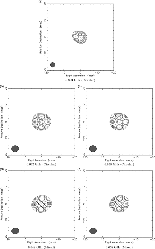
Appendix E. Polarisation images for all AGN target sources
The polarisation images created without Mp for all eight AGN target sources from the experiments VT23A and VT23B for two IFs of Circular and Mixed data are illustrated in Figures 7–14. In general, the same imaging parameters as in Figure 5 are used here; more appropriate parameters used for some particular images are mentioned within the parentheses in the captions.
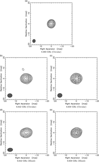
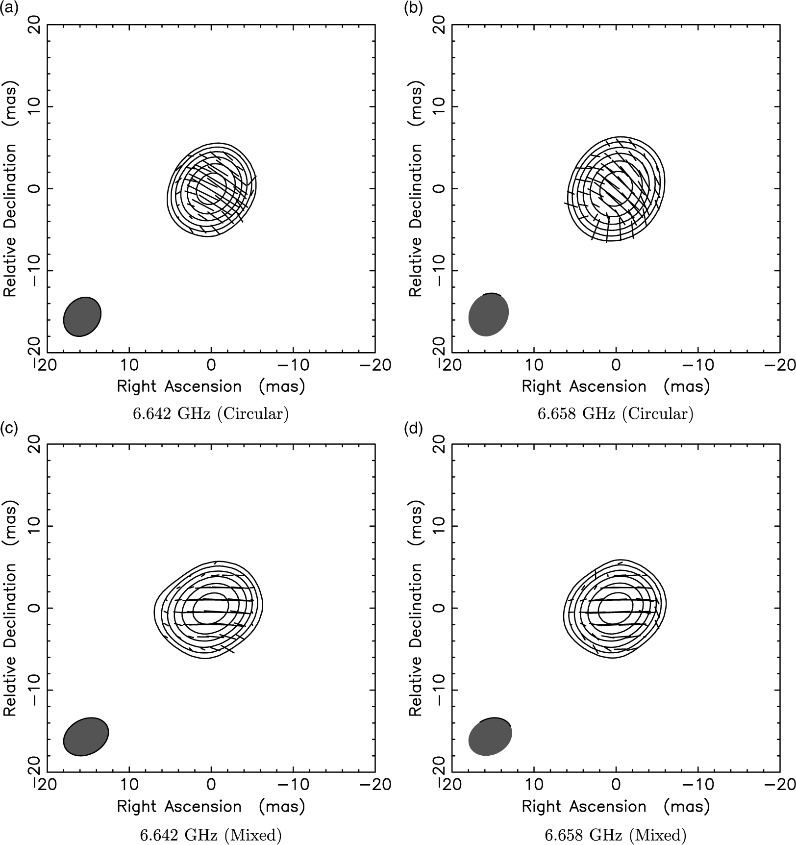
The 0135−247 polarisation maps for Circular data at 8.393 GHz (a), 6.642 GHz (b), and 6.658 GHz (c) and Mixed data at 6.642 GHz (d) and 6.658 GHz (e) [for (a), linear polarisation vectors are set to 1 asec/Jy].

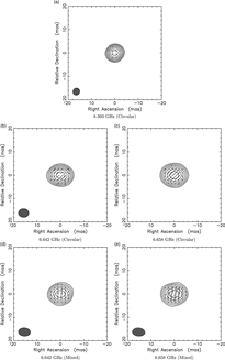
The 0142−278 polarisation maps for Circular data at 8.393 GHz (a), 6.642 GHz (b), and 6.658 GHz (c) and Mixed data at 6.642 GHz (d) and 6.658 GHz (e) [for all images, contour levels are set to −2%, 2%, 4%, 6%, 8%, 16%, 32%, and 64% and for (a), linear polarisation vectors are set to 1 asec/Jy].

The 0227−369 polarisation maps for Circular data at 8.393 GHz (a), 6.642 GHz (b), and 6.658 GHz (c) and Mixed data at 6.642 GHz (d) and 6.658 GHz (e) (for all images, linear polarisation vectors are set to 1 asec/Jy).

The 0234−301 polarisation maps for Circular data at 8.393 GHz (a), 6.642 GHz (b), and 6.658 GHz (c) and Mixed data at 6.642 GHz (d) and 6.658 GHz (e) [for (d) and (e), contour levels are set to −2%, 2%, 4%, 6%, 8%, 16%, 32%, and 64% and for (a), linear polarisation vectors are set to 1 asec/Jy].

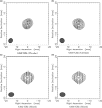
The 0146+056 polarisation maps for Circular data at 6.642 GHz (a) and 6.658 GHz (b) and Mixed data at 6.642 GHz (c) and 6.658 GHz (d) (for all images, contour levels are set to −2%, 2%, 4%, 6%, 8%, 16%, 32%, and 64%).
The 0237+040 polarisation maps for Circular data at 6.642 GHz (a) and 6.658 GHz (b) and Mixed data at 6.642 GHz (c) and 6.658 GHz (d) (for all images, contour levels are set to −3%, 3%, 6%, 12%, 24%, 48%, and 96%).

The 0426−380 polarisation maps for Circular data at 6.642 GHz (a) and 6.658 GHz (b) and Mixed data at 6.642 GHz (c) and 6.658 GHz (d) (for all images, linear polarisation vectors are set to 200 mas/Jy and for (c) and (d), contour levels are set to −3%, 3%, 6%, 12%, 24%, 48%, and 96%, and polarisation vectors are plotted where Stokes I fluxes are >200 mJy.

The 0451−282 polarisation maps for Circular data at 6.642 GHz (a) and 6.658 GHz (b) and Mixed data at 6.642 GHz (c) and 6.658 GHz (d) [for (c) and (d), contour levels are set to −2%, 2%, 4%, 6%, 8%, 16%, 32%, and 64% and for (d), polarisation vectors are plotted where Stokes I fluxes are >90 mJy.]