





1 Introduction
In the context of computerized testing, response times (RTs) have become widely used as an important auxiliary information for detecting various types of aberrant test-taking behaviors. Researchers have explored the use of RTs to identify test speededness (Schnipke & Scrams, Reference Schnipke and Scrams1997; van decr Linden et al., Reference van der Linden, Scrams and Schnipke1999), item pre-knowledge (van der Linden & Guo, Reference van der Linden and Guo2008), and low motivation or lack of effort (Wise & Kong, Reference Wise and Kong2005). Among these, test speededness is particularly noteworthy, as it occurs when time limits impact examinees’ performance, even though speed is not a construct that the test aims to measure (Shao et al., Reference Shao, Li and Cheng2016). Test speededness can lead to a decrease in response accuracy, particularly toward the end of the test, or result in missing responses (Goegebeur et al., Reference Goegebeur, De Boeck and Molenberghs2010). Additionally, it may distort the estimation of both item parameters and latent abilities (Douglas et al., Reference Douglas, Kim, Habing and Gao1998; Lu et al., Reference Lu, Wang, Zhang and Wang2024), thereby threatening the validity of the test results. Moreover, the presence of speededness can change or diminish the relationship between the test scores and other relevant factors (Cheng & Shao, Reference Cheng and Shao2022). To ensure the security and reliability of the test, it is therefore crucial to identify and address response patterns influenced by test speededness.
To address the challenges posed by test speededness, various methods have been proposed to detect test speededness using RTs. The first detection method is based on residual analysis. This method involves constructing a parametric model for RTs, such as the lognormal model proposed by van der Linden (Reference van der Linden2006). It then determines whether test speededness exists by comparing the differences between predicted RTs and observed RTs. Specifically, an examinee can be considered to exhibit test speededness if their observed RT significantly deviates from the model’s predicted value, which is typically indicated by large residuals that are statistically different from zero and exceed a predefined threshold, such as several standard deviations (van der Linden & van Krimpen-Stoop, Reference van der Linden and van Krimpen-Stoop2003).
The second method involves constructing a mixture hierarchical model or using a latent class model to detect test speededness, particularly rapid guessing behavior, which is a form of test speededness. Specifically, Wang and Xu (Reference Wang and Xu2015) adopted a mixture model to simultaneously consider RTs and response accuracy, aiming to distinguish between two primary behaviors that test-takers may exhibit during the test: solution behavior and rapid guessing behavior. Solution behavior typically occurs when test-takers carefully consider each question, whereas rapid guessing behavior typically arises under time pressure or lack of effort, resulting in hurriedly answering the remaining items, with their responses being close to random chance. In addition, Fox and Marianti (Reference Fox and Marianti2016) proposed another method by constructing a latent growth model to account for variable working speed. The premise of this model is that a test-taker’s response speed is not constant throughout the test. By introducing random effects to model each test-taker’s speed process, this model allows test-takers to adjust response speed during the test, which may manifest as linear or quadratic growth. The goal of this method is to capture changes in response speed at different stages of the test.
The third method for detecting test speededness is changepoint analysis (CPA). This approach identifies significant shifts in RT patterns, particularly changes in a test taker’s working speed. The main purpose of CPA is to determine whether a changepoint exists, which indicates a noticeable shift in working speed that is usually reflected in RTs. In the likelihood ratio test (LRT) version of CPA, the LRT compares the likelihoods of two models. The null hypothesis assumes constant speed (no changepoint), and the alternative hypothesis assumes a speed change at a certain point. A significant likelihood ratio indicates a change in speed, and the changepoint location can be estimated by selecting the point that maximizes the LRT statistic (Cheng & Shao, Reference Cheng and Shao2022; Shao et al., Reference Shao, Li and Cheng2016; Sinharay, Reference Sinharay2016). The Wald test directly compares the estimated working speeds before and after the changepoint to evaluate whether the difference is significant (Cheng & Shao, Reference Cheng and Shao2022; Sinharay, Reference Sinharay2016). The score test evaluates whether working speed differs across stages by examining the ratio of the first derivative of the log likelihood function with respect to the speed parameter to the corresponding Fisher information (Sinharay, Reference Sinharay2017). More recently, Lu et al. (Reference Lu, Wang, Zhang and Liu2026) proposed three Schwarz information criterion (SIC)-based CPA procedures using responses only, RTs only, or both jointly, and showed that the joint procedure generally achieved the best overall performance for detecting test speededness, while the SIC-based CPA procedures were also computationally more efficient than the likelihood ratio and Wald tests.
Within the general CPA framework, the cumulative sum (CUSUM) procedure is one of the most widely used methods. Originally proposed by Page (Reference Page1954), CUSUM has been extensively applied in statistical process control and CPA, where it has proven particularly effective for detecting small shifts in the mean of measured variables. Its sensitivity to small changes has made CUSUM an important tool in many statistical applications. Over time, both the theoretical foundations and practical implementations of CUSUM have been further developed in recent studies (Ciuperca, Reference Ciuperca2017; Gao et al., Reference Gao, Yang, Li and Yao2025; Sinharay, Reference Sinharay2016; Wang & Ning, Reference Wang and Ning2025; Yu & Cheng, Reference Yu and Cheng2022). In the field of educational and psychological measurement, the CUSUM method has also demonstrated strong potential when applied to item response data. For example, Sinharay (Reference Sinharay2016) proposed three CPA-based statistics and compared them with four CUSUM-based indices. Yu and Cheng (Reference Yu and Cheng2022) later conducted a systematic evaluation of 12 CUSUM-based statistics and 3 CPA-based procedures for detecting test speededness.
In CUSUM-based changepoint detection, the choice of critical value is critical, as it directly affects the sensitivity and specificity of the test. Several methods have been proposed for calculating critical values to infer test speededness. For instance, Shao et al. (Reference Shao, Li and Cheng2016) derived critical values for the LRT statistic through data permutation, while Sinharay (Reference Sinharay2016) relied on asymptotic results (Andrews, Reference Andrews1993), and Worsley (Reference Worsley1979) and Yu and Cheng (Reference Yu and Cheng2022) employed Monte Carlo simulations. However, these traditional methods have notable limitations in practice. Permutation methods can be computationally intensive for long tests or large samples, and they require that the null hypothesis holds when estimating critical values; if the data actually contain a changepoint, the method may fail. In contrast, asymptotic methods and Monte Carlo simulations require a priori assumptions about the underlying data distribution, and critical values are estimated based on these assumed distributions. Asymptotic critical values may also be inaccurate when changepoints occur near boundaries (Andrews, Reference Andrews1993; Sinharay, Reference Sinharay2016), while Monte Carlo simulations, though flexible, are less efficient near critical points, making it difficult to obtain precise thresholds (Singha et al., Reference Singha, Chakrabarti and Arora2023).
To address these limitations, the Bootstrap method has been increasingly adopted to estimate the empirical distribution of the CUSUM statistic, thereby obtaining the critical value for the test. Unlike traditional methods, Bootstrap does not require any assumptions about the data distribution. Moreover, even when the null hypothesis is not strictly valid, the multiplier Bootstrap can still be used to estimate the empirical distribution of the CUSUM statistic, providing a robust and flexible way to determine critical values. For example, Yu and Chen (Reference Yu and Chen2021) applied the multiplier Bootstrap to a high-dimensional mean-change model, ensuring theoretical validity and consistency when detecting single or multiple changepoints. Similarly, Horowitz and Savin (Reference Horowitz and Savin2000) demonstrated that the multiplier Bootstrap can substantially reduce bias in finite samples, improving the accuracy of critical value estimation.
Building on existing research, our study proposes an innovative Bootstrap-CUSUM CPA method for detecting test speededness in examinees’ RT data. We construct an individual-level CUSUM statistic based on RT data and employ the multiplier Bootstrap method to estimate its empirical distribution. This makes it possible to determine the critical value based on the empirical distribution, without relying on specific distributional assumptions for RTs or on the asymptotic normality of the CUSUM statistic. The procedure is applied to each examinee to obtain an individual-specific critical value, and the averaged critical value across examinees is then computed. When an examinee’s CUSUM statistic exceeds this averaged critical value, they are identified as exhibiting test speededness, and the specific item at which this behavior begins can be pinpointed. Our method enables the simultaneous detection of test speededness for each examinee and the estimation of changepoint locations. This approach not only allows for a more detailed and flexible analysis of test speededness, but also provides a methodologically rigorous and empirically grounded tool for studying test-taking behavior.
Strengths of the Bootstrap-CUSUM method in detecting test speededness
Bootstrap-CUSUM offers several key advantages over residual analysis, mixture models, latent growth models, and CPA methods (including LRT, Wald, and score tests) when detecting test speededness. These advantages arise not only from its data-driven nature but also from its ability to effectively control false positives, provide accurate changepoint estimation, ensure theoretical consistency, and adapt to the complexities of real-world data.
Traditionally, residual analysis and CPA methods typically require a pre-specified RT distribution model (e.g., the lognormal model) or a joint response and RT model. While these methods allow for interpretability through model parameters, their performance is highly sensitive to the correctness of distributional and structural assumptions. If the true data distribution deviates from these assumptions, the statistical properties may be distorted, leading to inflated Type I error rates, reduced statistical power, or even misclassification of results (Berk, Reference Berk1966; Box, Reference Box1953). Furthermore, mixture models and latent growth models are explicit modeling methods used to detect test speededness. Their primary advantage is their direct ability to model and interpret changes in response speed. However, these models are heavily dependent on accurate model specification. For instance, the number of latent classes, the functional form of growth curves, and the covariance structure must either be pre-specified or determined through complex model selection procedures. Misspecification in any of these areas can lead to poor model fit, incorrect classifications, or biased test-taking behavior trajectory estimates (Nylund et al., Reference Nylund, Asparouhov and Muthen2007). Moreover, these methods often require large sample sizes for stable estimation; when the number of examinees or items is small, model convergence can be unstable, and parameter estimates may exhibit large variances.
Compared to the methods discussed above, the Bootstrap-CUSUM method offers several distinct advantages. First, the Bootstrap-CUSUM method does not require specifying a particular parametric distribution on RTs, although it does require the item time intensity parameters to be relatively homogeneous so that changes in observed RTs can interpreted as changes in speed. More importantly, its critical values are not derived from a parametric reference distribution or from the asymptotic normality of the CUSUM statistic. Instead, they are obtained through a multiplier bootstrap that directly approximates the empirical sampling distribution of the extreme-value statistic $K_{i}$
conditional on the observed sequence. This allows the procedure to avoid relying on asymptotic normal approximations and to adapt, to some extent, to irregular tail behavior and data fluctuations in practice. Second, unlike traditional methods, it does not require explicit specification of latent speed classes or functional forms, which enhances its adaptability to diverse data characteristics. This flexibility allows the method to be applied to RT data under broader distributional conditions, including complex or misspecified distributions, making it a more robust tool in practical settings where distributional assumptions are often violated. Furthermore, the method avoids parameter estimation, which mitigates the risk of inference errors due to parameter misspecification. Traditional methods typically rely on parameter estimates based on predefined models, which can lead to inaccurate conclusions if the model assumptions are not fully satisfied. In contrast, the Bootstrap-CUSUM method is entirely data-driven: for each examinee, RTs (typically log-transformed to stabilize variance) are analyzed using a mean-shift changepoint model to compute the maximum CUSUM statistic. This method allows for a more adaptive and accurate representation of the data. Given that the null distribution of the CUSUM statistic is analytically intractable, the Bootstrap-CUSUM method employs the multiplier bootstrap to empirically approximate its distribution and estimate the critical value. This resampling-based approach avoids reliance on closed-form distributional assumptions and is less sensitive to non-normality in log-RTs. The ability to obtain critical values empirically further enhances the robustness of the method, particularly in complex real-world settings.
$K_{i}$
conditional on the observed sequence. This allows the procedure to avoid relying on asymptotic normal approximations and to adapt, to some extent, to irregular tail behavior and data fluctuations in practice. Second, unlike traditional methods, it does not require explicit specification of latent speed classes or functional forms, which enhances its adaptability to diverse data characteristics. This flexibility allows the method to be applied to RT data under broader distributional conditions, including complex or misspecified distributions, making it a more robust tool in practical settings where distributional assumptions are often violated. Furthermore, the method avoids parameter estimation, which mitigates the risk of inference errors due to parameter misspecification. Traditional methods typically rely on parameter estimates based on predefined models, which can lead to inaccurate conclusions if the model assumptions are not fully satisfied. In contrast, the Bootstrap-CUSUM method is entirely data-driven: for each examinee, RTs (typically log-transformed to stabilize variance) are analyzed using a mean-shift changepoint model to compute the maximum CUSUM statistic. This method allows for a more adaptive and accurate representation of the data. Given that the null distribution of the CUSUM statistic is analytically intractable, the Bootstrap-CUSUM method employs the multiplier bootstrap to empirically approximate its distribution and estimate the critical value. This resampling-based approach avoids reliance on closed-form distributional assumptions and is less sensitive to non-normality in log-RTs. The ability to obtain critical values empirically further enhances the robustness of the method, particularly in complex real-world settings.
In addition, the proposed Bootstrap-CUSUM method offers several notable advantages in theoretical properties, the detection of test speededness, and changepoint estimation. First, in terms of the theoretical properties, the Bootstrap-CUSUM method provides separate consistency guarantees for its two inference steps. Under the null hypothesis, the multiplier bootstrap distribution converges to the true sampling distribution in large samples, thereby ensuring accurate control of the significance level. Under the alternative hypothesis, we establish that the changepoint estimator obtained by maximizing the CUSUM statistic converges in probability to the true changepoint location, thus providing rigorous theoretical guarantees for localization accuracy. Second, in terms of detecting test speededness, comprehensive performance comparisons based on simulation studies conducted under multiple distributional conditions, as well as varying test lengths and proportions of speededness, indicate that the Bootstrap-CUSUM method consistently achieves the highest correct classification rate (CCR), the lowest false positive rate (FPR), and a true detection rate (TDR) comparable to or superior to that of competing methods. This demonstrates a well-balanced performance characterized by high accuracy and low false alarm rates. Moreover, the Bootstrap-CUSUM method avoids reliance on complex latent structures (e.g., the number of classes or the form of growth trajectories), requiring only the observed RT sequence for analysis. This substantially reduces the impact of model misspecification on inference results, while its computation remains straightforward. This method not only maintains broad applicability across different distributional forms of RT data, but also accounts for heteroscedasticity in the error term. In contrast, traditional approaches, such as model-based residual analysis, mixture models, latent growth models, as well as LRTs, score tests, and Wald tests, often require additional steps or adjustments to ensure that the data satisfy their underlying statistical assumptions. Finally, with respect to changepoint estimation, the Bootstrap-CUSUM method can also pinpoint the location of the changepoints. When examinee is identified as exhibiting test speededness, the location of the changepoint can be estimated by maximizing the test statistic. This feature enables the method not only to detect test speededness at individual level but also to accurately pinpoint the item location at which it occurs.
The remainder of this article is organized as follows. In Section 2, changepoint detection models are introduced. Section 3 introduces the proposed Bootstrap-CUSUM method, detailing the formulation of the CUSUM statistic, the computation of critical values via the multiplier bootstrap, and the estimation of changepoint locations in log-RTs. Section 4 establishes the consistency of the Bootstrap-CUSUM method for estimating both the critical value and the changepoint location under the null and alternative hypotheses. Section 5 presents four simulation studies assessing the detection performance of the proposed method under three RT distributions: multivariate normal, multivariate t, and contaminated Gaussian, including gradual and abrupt changepoint scenarios, heterogeneity in item time-intensity parameters, and different critical value selection strategies. Section 6 provides an empirical data analysis. Finally, Section 7 concludes with a summary of the findings, a discussion of strengths and limitations, and future research directions.
2 Changepoint analysis models
In this section, we introduce the generalized heteroskedastic mean-shift log-RT (GHMS-LRT) model for detecting test speededness. Before formally presenting this model, we first provide a brief review of the log-normal RT model.
2.1 Log-normal response time model
van der Linden (Reference van der Linden2006) proposed a lognormal model for RTs. Let $T_{ij}$
represent the RT of examinee i (i = 1, …, n) on item j (j = 1, …, J).
$T_{ij}$
represent the RT of examinee i (i = 1, …, n) on item j (j = 1, …, J). $T_{ij}$
is assumed to follow a lognormal distribution:
$T_{ij}$
is assumed to follow a lognormal distribution:
 $$ \begin{align} \log(T_{ij})=\beta_{j}-\tau_{i}+\epsilon_{ij},\quad\epsilon_{ij}\sim N\left( 0,\sigma_{j}^{2}\right) , \end{align} $$
where $\tau _{i}$
denotes the latent speed parameter of the ith examinee, with larger values corresponding to faster responses. The parameter
$\tau _{i}$
denotes the latent speed parameter of the ith examinee, with larger values corresponding to faster responses. The parameter $\beta _{j}$
characterizes the time intensity of item j, where a greater
$\beta _{j}$
characterizes the time intensity of item j, where a greater $\beta _{j}$
indicates that the item requires more time to complete.
$\beta _{j}$
indicates that the item requires more time to complete. $\sigma _{j}^{2}$
quantifies the dispersion of the lognormal distribution.
$\sigma _{j}^{2}$
quantifies the dispersion of the lognormal distribution.
2.2 Generalized heteroskedastic mean-shift log-RT model
Within the framework of van der Linden’s (Reference van der Linden2006) lognormal RT model, the GHMS-LRT model is used to detect test speededness. The GHMS-LRT model extends the traditional lognormal RT model by embedding it into a heteroskedastic mean-shift structure, thereby enabling flexible distributional assumptions while explicitly modeling test speededness through changepoint detection.
For a given examinee i, the GHMS-LRT model is specified as
 $$ \begin{align} \log(T_{ij}) = \beta_j - \tau_i + \delta_i I(j> m_i) + \epsilon_{ij}, \quad i=1, \ldots , n;\quad j = 1, \ldots, J, \end{align} $$
where $m_i \in \{2, 3, \ldots , J-2\}$
denotes the changepoint location for examinee i, and
$m_i \in \{2, 3, \ldots , J-2\}$
denotes the changepoint location for examinee i, and $\delta _i$
is an individual-level shift parameter indicating whether examinee i exhibits test speededness. If
$\delta _i$
is an individual-level shift parameter indicating whether examinee i exhibits test speededness. If $\delta _i = 0$
, the RT sequence contains no changepoint, indicating stable responding, and we set
$\delta _i = 0$
, the RT sequence contains no changepoint, indicating stable responding, and we set $m_i = J$
. If
$m_i = J$
. If $\delta _i < 0$
, the mean log-RT decreases after
$\delta _i < 0$
, the mean log-RT decreases after $m_i$
, implying acceleration and thus the presence of test speededness. In this case, the examinee is assumed to respond at a normal speed to items
$m_i$
, implying acceleration and thus the presence of test speededness. In this case, the examinee is assumed to respond at a normal speed to items $1,\ldots ,m_i$
, and to exhibit test speededness from item
$1,\ldots ,m_i$
, and to exhibit test speededness from item $m_i + 1$
to item J.
$m_i + 1$
to item J.
Accordingly, the hypotheses for detecting test speededness in examinee i are formulated as
 $$ \begin{align} \mathcal{H}_0: \delta_i = 0 \quad \text{(no test speededness)} \qquad \text{vs.} \qquad \mathcal{H}_1: \delta_i < 0 \quad \text{(test speededness present)}. \end{align} $$
Remark. In model (2), we assume that the item time intensity parameters $\beta _j$
are relatively homogeneous across items. That is, item time intensities fluctuate only slightly to moderately around a common mean and do not, by themselves, induce noticeable changes in the RT sequence. In other words, although
$\beta _j$
are relatively homogeneous across items. That is, item time intensities fluctuate only slightly to moderately around a common mean and do not, by themselves, induce noticeable changes in the RT sequence. In other words, although $ \beta _j $
may vary within a certain range across items, such variation should not be large enough to create essentially shift in response speed described in model (2), such as the two distinct speed levels between the first
$ \beta _j $
may vary within a certain range across items, such variation should not be large enough to create essentially shift in response speed described in model (2), such as the two distinct speed levels between the first $ m_i $
items (i.e.,
$ m_i $
items (i.e., $\tau _i$
) and the remaining
$\tau _i$
) and the remaining $J - m_i$
items when
$J - m_i$
items when $\delta _i < 0 $
(i.e.,
$\delta _i < 0 $
(i.e., $\tau _i-\delta _i$
). Thus, when the time intensities
$\tau _i-\delta _i$
). Thus, when the time intensities $\beta _j$
are relatively homogeneous, changepoint detection for the log RT sequence in the changepoint model (2) can be approximately reduced to detecting changes in the individual speed parameter
$\beta _j$
are relatively homogeneous, changepoint detection for the log RT sequence in the changepoint model (2) can be approximately reduced to detecting changes in the individual speed parameter $\tau _i$
.
$\tau _i$
.
This assumption is also consistent with common simulation designs in the existing literature, researchers typically generate $\beta _j$
from distributions with small variance, yielding homogeneous time intensity parameters. For example, Lu et al. (Reference Lu, Wang, Zhang and Tao2020) set the variance of
$\beta _j$
from distributions with small variance, yielding homogeneous time intensity parameters. For example, Lu et al. (Reference Lu, Wang, Zhang and Tao2020) set the variance of $\beta _j $
to 0.2. Cheng and Shao (Reference Cheng and Shao2022), when constructing likelihood ratio and Wald tests based on RTs to detect test speededness, followed previous work and further fixed the variance strictly at
$\beta _j $
to 0.2. Cheng and Shao (Reference Cheng and Shao2022), when constructing likelihood ratio and Wald tests based on RTs to detect test speededness, followed previous work and further fixed the variance strictly at $ 1/9\approx 0.111 $
. In addition, Wang and Xu (Reference Wang and Xu2015) assess the performance of mixture model under different levels of time intensity parameters, they generated
$ 1/9\approx 0.111 $
. In addition, Wang and Xu (Reference Wang and Xu2015) assess the performance of mixture model under different levels of time intensity parameters, they generated $\beta _j$
from the three uniform distributions
$\beta _j$
from the three uniform distributions $U(-0.25,0.25) $
,
$U(-0.25,0.25) $
, $ U(0,0.5) $
, and
$ U(0,0.5) $
, and $ U(0.25,0.75) $
, each with variance
$ U(0.25,0.75) $
, each with variance $1/48\approx 0.021$
. In this study, to evaluate the effectiveness of the proposed method and the feasibility of the homogeneous assumption on
$1/48\approx 0.021$
. In this study, to evaluate the effectiveness of the proposed method and the feasibility of the homogeneous assumption on $ \beta _j $
, we consider two fluctuation scenarios: Simulation Study I sets the variance of
$ \beta _j $
, we consider two fluctuation scenarios: Simulation Study I sets the variance of $ \beta _j $
to 0.2, whereas Simulation Study II follows Wang and Xu (Reference Wang and Xu2015) and draws
$ \beta _j $
to 0.2, whereas Simulation Study II follows Wang and Xu (Reference Wang and Xu2015) and draws $ \beta _j $
from the three uniform distributions described above, each with variance
$ \beta _j $
from the three uniform distributions described above, each with variance $1/48\approx 0.021$
.
$1/48\approx 0.021$
.
Note that the relative homogeneity condition does not require $\beta _j$
to be exactly equal across all items or to have an extremely small variance. Instead, the key requirement is that
$\beta _j$
to be exactly equal across all items or to have an extremely small variance. Instead, the key requirement is that $\beta _j$
should not exhibit pronounced ordered or segmented structural changes along the item sequence; otherwise, item characteristics may induce a systematic drift that resembles a changepoint, thereby confounding item-driven changes with speed-change signals. Before applying our method, users may conduct simple diagnostics of the data and test structure to assess whether structural heterogeneity in item time intensity is likely. Specifically, (1) checking whether item types are highly consistent (e.g., all multiple-choice or all constructed-response items); (2) checking whether item types or reading passages appear in “blocks” or in an obviously segmented order along the test; and (3) if a substantial risk of structural segmentation exists, considering stratified analyses by item type or adjusting for item-order effects.
$\beta _j$
should not exhibit pronounced ordered or segmented structural changes along the item sequence; otherwise, item characteristics may induce a systematic drift that resembles a changepoint, thereby confounding item-driven changes with speed-change signals. Before applying our method, users may conduct simple diagnostics of the data and test structure to assess whether structural heterogeneity in item time intensity is likely. Specifically, (1) checking whether item types are highly consistent (e.g., all multiple-choice or all constructed-response items); (2) checking whether item types or reading passages appear in “blocks” or in an obviously segmented order along the test; and (3) if a substantial risk of structural segmentation exists, considering stratified analyses by item type or adjusting for item-order effects.
The error term $\epsilon _{ij}$
is introduced to capture random variation in log-RTs. Our model does not assume any specific distribution for
$\epsilon _{ij}$
is introduced to capture random variation in log-RTs. Our model does not assume any specific distribution for $\epsilon _{ij}$
; it only requires that
$\epsilon _{ij}$
; it only requires that $E(\epsilon _{ij})=0$
and
$E(\epsilon _{ij})=0$
and $Var(\epsilon _{ij})={\sigma _{j}}$
. Nevertheless, because RT data are typically positive, right-skewed, and heterogeneous across items, adopting flexible and robust distributional forms can better accommodate different data characteristics. Accordingly, we allow
$Var(\epsilon _{ij})={\sigma _{j}}$
. Nevertheless, because RT data are typically positive, right-skewed, and heterogeneous across items, adopting flexible and robust distributional forms can better accommodate different data characteristics. Accordingly, we allow $\boldsymbol {\epsilon }_{i}=\left (\epsilon _{i1}, \epsilon _{i2}, \dots , \epsilon _{iJ}\right )^{\text {T}}$
to follow one of the following distributions:
$\boldsymbol {\epsilon }_{i}=\left (\epsilon _{i1}, \epsilon _{i2}, \dots , \epsilon _{iJ}\right )^{\text {T}}$
to follow one of the following distributions:
-
1. Multivariate normal distribution: Appropriate when RTs are approximately symmetric after log-transformation, with moderate variability across items. Assume that the random error term $\boldsymbol {\epsilon }_{i}\sim MVN(\boldsymbol {0}, \boldsymbol {V})$
, where
$\boldsymbol {V}=diag(\sigma _{1}^2,\sigma _{2}^2,\ldots ,\sigma _{J}^2)$
.
$\boldsymbol {\epsilon }_{i}\sim MVN(\boldsymbol {0}, \boldsymbol {V})$
, where
$\boldsymbol {V}=diag(\sigma _{1}^2,\sigma _{2}^2,\ldots ,\sigma _{J}^2)$
. -
2. Multivariate t distribution: Suitable for heavy-tailed RT data, where some items or examinees may produce unusually long RTs that deviate from the bulk of the data. Assume that the random error term
$\boldsymbol {\epsilon }_{i}$
follows a J-dimensional multivariate t-distribution with degrees of freedom
$v>0$
and a positive-definite scale matrix
$\boldsymbol {V}$
, denoted as
$\boldsymbol {\epsilon }_{i} \sim t_{v}(\mathbf {0}, \boldsymbol {V})$
with the probability density function (4)
$$ \begin{align} f(\boldsymbol{x};v,\boldsymbol{V}) = \frac{\Gamma\left(\frac{v+J}{2}\right)}{\Gamma\left(\frac{v}{2}\right) (\pi v)^{J/2} \det(\boldsymbol{V})^{1/2}} \left( 1 + \frac{\boldsymbol{x}^{\top} \boldsymbol{V}^{-1} \boldsymbol{x}}{v} \right)^{-\frac{v+J}{2}}. \end{align} $$
When
$v>2$
, the covariance matrix of
$\boldsymbol {\epsilon }_{i}$
exists and is given by
$$\begin{align*}\boldsymbol{\Sigma} = \frac{v}{v-2} \, \boldsymbol{V}. \end{align*}$$
In practical applications, it is rare for data to conform strictly to normality. Compared with the multivariate normal distribution, the multivariate t distribution has heavier tails, meaning that its probability mass decays more slowly in the extremes. This heavy-tailed property reduces the influence of aberrant or extreme observations on CPA, thereby improving the accuracy of changepoint detection. In educational and psychological assessments, the test length for an individual examinee is often finite (referred to as finite-sample). The degrees-of-freedom parameter of the multivariate t distribution can be flexibly tuned, enabling it to more accurately approximate the true data distribution while maintaining high robustness under conditions of finite-sample and distributional uncertainty.
-
3. Contaminated Gaussian distribution: A flexible mixture model designed to represent situations in which normal and aberrant observations coexist within the data. Let the random error term
$\boldsymbol {\epsilon }_{i}$
follow a contaminated Gaussian distribution, denoted as
$\mathrm {ctm\mbox {-}Gaussian}(\varphi ,v,\boldsymbol {V})$
, with contamination proportion
$\varphi \in [0,1]$
, degrees of freedom v, and scale matrix
$\boldsymbol {V}$
. Its probability density function is given by (5)
$$ \begin{align} f(\boldsymbol{x};\varphi,v,\boldsymbol{V})=(1-\varphi)\frac{\exp\!\left( -\tfrac{1} {2}\boldsymbol{x}^{\top}\boldsymbol{V}^{-1}\boldsymbol{x}\right) } {(2\pi)^{J/2}\det(\boldsymbol{V})^{1/2}}+\varphi\,\frac{\Gamma\!\left( \tfrac{v+J}{2}\right) }{\Gamma\!\left( \tfrac{v}{2}\right) (\pi v)^{J/2}\det(\boldsymbol{V})^{1/2}}\left( 1+\frac{\boldsymbol{x}^{\top }\boldsymbol{V}^{-1}\boldsymbol{x}}{v}\right) ^{-\tfrac{v+J}{2}}. \end{align} $$
Equation (5) shows that contaminated Gaussian distribution is a convex combination of the multivariate normal distribution
$\mathit {MVN} (\mathbf {0},\boldsymbol {V})$
and the multivariate t distribution
$t_{v}(\boldsymbol {V})$
, with
$\varphi $
governing the contamination proportion. The covariance matrix of
$\boldsymbol {\epsilon }_{i}$
is ensuring a finite covariance structure when
$$\begin{align*}\boldsymbol{\Sigma}=\Big[(1-\varphi)+\varphi\tfrac{v}{v-2}\Big]\boldsymbol{V},\quad v>2, \end{align*}$$
$v>2$
.
The contaminated Gaussian distribution is an extension of the multivariate normal distribution that more effectively accommodates the non-standard scenarios commonly encountered in practice. It can be broadly applied across various statistical contexts, including clustering, detection of aberrant observations, and latent variable modeling (Punzo & Tortora, Reference Punzo and Tortora2021; Tomarchio et al., Reference Tomarchio, Gallaugher, Punzo and McNicholas2022). This distribution is particularly well-suited to situations where data contain aberrant or noisy observations, allowing for a more accurate representation of the underlying data distribution.


It should be noted that the three distributions mentioned in this article for the error term, namely, the multivariate normal distribution, the multivariate t distribution, and the contaminated Gaussian distribution, are not intended as distributional assumptions for parametric inference. Instead, they are used to construct simulated data scenarios with different tail properties and variability, to systematically evaluate the performance and robustness of the proposed method under various data-generating mechanisms. In other words, the proposed method does not rely on any specific form of data distribution. These distributions are used solely for data generation in simulation studies and are not distributional assumptions required for applying the proposed method. Accordingly, the method does not require recovering these distributions. This distinguishes the proposed method from traditional parametric approaches and constitutes one of its main advantages.
3 Bootstrap-CUSUM method
To determine whether a changepoint exists in an examinee’s log-RTs under the GHMS-LRT model (Equation (2)), this section introduces the CUSUM statistic to measure changes in response speed across the examinee’s RT sequence and presents the implementation of the multiplier Bootstrap method for estimating the critical value for the test.
3.1 CUSUM statistic
To investigate potential changes in the RT characteristics of examinees, we partition the RT sequence of the i-th examinee at the s-th item location. The resulting subsets are defined as Subset 1 $\left (T_{i1}, T_{i2}, \ldots , T_{is}\right )$
and Subset 2
$\left (T_{i1}, T_{i2}, \ldots , T_{is}\right )$
and Subset 2 $\left (T_{i\left (s+1\right )}, T_{i\left (s+2\right )}, \ldots , T_{iJ}\right )$
, as illustrated in Figure 1.
$\left (T_{i\left (s+1\right )}, T_{i\left (s+2\right )}, \ldots , T_{iJ}\right )$
, as illustrated in Figure 1.
Response time segmentation for the i-th examinee, illustrating the partition between subset 1 and subset 2 at the item location s (i.e., partition point).

If examinee i does not exhibit test speededness, then after partitioning at any location s, the means of the two resulting subsets should remain approximately equal. To conduct the hypothesis testing, we construct a CUSUM statistic. For examinee i, given the log RT sequence $\left \{\log T_{i1},\log T_{i2},\ldots ,\log T_{iJ}\right \}$
, define the cumulative deviation up to item location s as
$\left \{\log T_{i1},\log T_{i2},\ldots ,\log T_{iJ}\right \}$
, define the cumulative deviation up to item location s as
 $$ \begin{align} {\Delta}_{i}(s)=\sum_{j=1}^{s}\left( \log (T_{ij})-\overline{T_{i}}\right) ,\text{ where }\overline{T_{i}}=\frac{1}{J}\sum_{j=1}^{J}\log (T_{ij}). \end{align} $$
Normalizing by segment length yields the standardized CUSUM statistic:
 $$ \begin{align} Z_{i}(s) = \sqrt{\frac{J}{s(J-s)}} \, {\Delta}_{i}(s). \end{align} $$
Substituting the terms in Equation (7) by Equation (6) gives
 $$ \begin{align} Z_{i}(s)=\sqrt{\frac{J-s}{Js}}\sum_{j=1}^{s}\log (T_{ij})-\sqrt{\frac{s}{{J(J-s)}}}\sum_{j=s+1}^{J}\log (T_{ij}), \end{align} $$
which corresponds to Equation (8). Under $\mathcal {H}_{0}$
,
$\mathcal {H}_{0}$
, $Z_{i}(s)$
fluctuates around 0. A systematic departure of
$Z_{i}(s)$
fluctuates around 0. A systematic departure of $Z_{i}(s)$
from 0 indicates a significant difference between the means of the two subsets, suggesting a structural change in the log-transformed RT sequence.
$Z_{i}(s)$
from 0 indicates a significant difference between the means of the two subsets, suggesting a structural change in the log-transformed RT sequence.
Since the exact changepoint location s is unknown, it is necessary to evaluate all possible locations $s \in \{2,3,\ldots ,J-2\}$
. A localized deviation in
$s \in \{2,3,\ldots ,J-2\}$
. A localized deviation in $Z_i(s)$
may occur due to random noise; however, if a true changepoint exists, the deviation will be maximized near the actual shift. Therefore, the test statistic for the i-th examinee is defined as the maximum absolute value of the CUSUM statistic:
$Z_i(s)$
may occur due to random noise; however, if a true changepoint exists, the deviation will be maximized near the actual shift. Therefore, the test statistic for the i-th examinee is defined as the maximum absolute value of the CUSUM statistic:
 $$ \begin{align} {K}_i = \max_{s \in \{2,\ldots,J-2\}} |Z_i(s)|. \end{align} $$
This definition is supported by several reasons. First, because the changepoint location is unknown, taking the maximum across all s ensures that the strongest evidence of departure is captured without assuming prior knowledge of the changepoint. Second, the use of the absolute value allows the method to detect both acceleration (faster responses) and deceleration (slower responses) in RTs. Finally, in changepoint detection theory, the maximum of standardized CUSUM statistics is recognized as a well-established and powerful method for identifying structural breaks (Csörgö & Horváth, Reference Csörgö and Horváth1997; Page, Reference Page1954).
3.2 Multiplier bootstrap method
The key issue is how to determine the magnitude of the statistic $K_i$
and use it to assess whether an examinee exhibits test speededness. A common method is to set a critical value that distinguishes normal examinees from aberrant ones. In hypothesis testing, several methods have been proposed for obtaining critical values. For example, Shao et al. (Reference Shao, Li and Cheng2016) suggested deriving critical values for the LRT statistic through data permutation; Sinharay (Reference Sinharay2016) recommended using the asymptotic critical values provided by Andrews (Reference Andrews1993); and Worsley (Reference Worsley1979) and Yu and Cheng (Reference Yu and Cheng2022) employed Monte Carlo simulations to estimate critical values. However, these traditional methods have certain limitations in practice. Permutation methods are often computationally inefficient in the context of long tests; the applicability of asymptotic critical values may be restricted when the changepoint occurs at the beginning or the end of a test (Andrews, Reference Andrews1993; Sinharay, Reference Sinharay2016); and the efficiency of MCMC methods can decrease significantly near critical points, resulting in slow simulations (Singha et al., Reference Singha, Chakrabarti and Arora2023).
$K_i$
and use it to assess whether an examinee exhibits test speededness. A common method is to set a critical value that distinguishes normal examinees from aberrant ones. In hypothesis testing, several methods have been proposed for obtaining critical values. For example, Shao et al. (Reference Shao, Li and Cheng2016) suggested deriving critical values for the LRT statistic through data permutation; Sinharay (Reference Sinharay2016) recommended using the asymptotic critical values provided by Andrews (Reference Andrews1993); and Worsley (Reference Worsley1979) and Yu and Cheng (Reference Yu and Cheng2022) employed Monte Carlo simulations to estimate critical values. However, these traditional methods have certain limitations in practice. Permutation methods are often computationally inefficient in the context of long tests; the applicability of asymptotic critical values may be restricted when the changepoint occurs at the beginning or the end of a test (Andrews, Reference Andrews1993; Sinharay, Reference Sinharay2016); and the efficiency of MCMC methods can decrease significantly near critical points, resulting in slow simulations (Singha et al., Reference Singha, Chakrabarti and Arora2023).
To overcome these drawbacks, this study introduces the multiplier Bootstrap method to estimate critical values. Compared with traditional methods, this method offers several notable advantages. First, it can provide more accurate finite-sample critical values, which is particularly important for complex statistical models or finite-sample data. For instance, Horowitz and Savin (Reference Horowitz and Savin2000) demonstrated that the multiplier Bootstrap method substantially reduces finite-sample bias in obtaining critical values for hypothesis testing, thereby improving test accuracy. Second, traditional statistical inference methods often rely on assumptions that the data follow standard distributions, such as the normal or t-distribution. In contrast, the multiplier bootstrap method employs resampling techniques to construct the empirical distribution of a statistic directly from the observed sample, thereby avoiding inference bias that may arise when the population distribution deviates from traditional assumptions. This approach is particularly valuable for handling complex or non-standard data distributions and has been successfully applied to various sophisticated models, including U-processes and multivariate time series (Chen & Kato, Reference Chen and Kato2020; Kojadinovic & Yi, Reference Kojadinovic and Yi2024). Therefore, compared with traditional methods, the multiplier Bootstrap method exhibits greater flexibility and accuracy in determining critical values and is particularly suitable for the purposes of this study.
Let $Y_{i1}, Y_{i2}, \ldots , Y_{iJ}$
be independent random variables from the standard normal distribution
$Y_{i1}, Y_{i2}, \ldots , Y_{iJ}$
be independent random variables from the standard normal distribution $N(0,1)$
and independent of
$N(0,1)$
and independent of $\log (T_{i1}), \log (T_{i2}), \ldots , \log (T_{iJ})$
. Define the left and right means at the partition point
$\log (T_{i1}), \log (T_{i2}), \ldots , \log (T_{iJ})$
. Define the left and right means at the partition point
 $$\begin{align*}\bar{L}_{is}^{-}=\frac{1}{s}\sum_{j=1}^{s}\log(T_{ij})\quad \text{and}\quad \bar{L}_{is}^{+}=\frac{1}{J-s}\sum_{j=s+1}^{J}\log(T_{ij}). \end{align*}$$
Therefore, to construct the test statistic under the null hypothesis, we follow the approach of Yu and Chen (Reference Yu and Chen2021) and introduce the following multiplier Bootstrap-CUSUM statistic:
 $$ \begin{align} Z_{i}^{\ast}(s)=\sqrt{\frac{J-s}{Js}}\sum_{j=1}^{s}Y_{ij}\Big[\log (T_{ij})-\bar{L}_{is}^{-}\Big]-\sqrt{\frac{s}{J(J-s)}}\sum_{j=s+1}^{J} Y_{ij}\Big[\log(T_{ij})-\bar{L}_{is}^{+}\Big], \end{align} $$
and the corresponding maximum statistic is defined as $K_{i}^{*} = \max _{s \in \{2, \ldots , J-2\}} |Z_{i}^{*}(s)|$
. The implementation of the multiplier Bootstrap for estimating the critical value of the CUSUM statistic proceeds is as follows:
$K_{i}^{*} = \max _{s \in \{2, \ldots , J-2\}} |Z_{i}^{*}(s)|$
. The implementation of the multiplier Bootstrap for estimating the critical value of the CUSUM statistic proceeds is as follows:
Generate multipliers: For a given examinee i, in each bootstrap replication $b \in \{1, \ldots , B\}$
, we generate J independent random variables
$b \in \{1, \ldots , B\}$
, we generate J independent random variables $Y_{i1}^{(b)}, Y_{i2}^{(b)}, \ldots , Y_{iJ}^{(b)} \sim N(0,1)$
. These serve as multipliers to re-weight the centered log-RTs.
$Y_{i1}^{(b)}, Y_{i2}^{(b)}, \ldots , Y_{iJ}^{(b)} \sim N(0,1)$
. These serve as multipliers to re-weight the centered log-RTs.
Construct Bootstrap-CUSUM statistics: Using Equation (10), compute the Bootstrap-CUSUM statistic $Z_{i}^{*(b)}(s)$
for all partition points
$Z_{i}^{*(b)}(s)$
for all partition points $s \in \{2, \ldots , J-2\}$
and obtain the corresponding maximum
$s \in \{2, \ldots , J-2\}$
and obtain the corresponding maximum
 $$ \begin{align} K_{i}^{*(b)} = \max_{s \in \{2, \ldots, J-2\}} \big|Z_{i}^{*(b)}(s)\big|. \end{align} $$
Repeat Bootstrap resampling: Repeat the above two steps B times, producing a sequence $\{K_{i}^{*(1)}, K_{i}^{*(2)}, \ldots , K_{i}^{*(B)}\}$
that approximates the sampling distribution of
$\{K_{i}^{*(1)}, K_{i}^{*(2)}, \ldots , K_{i}^{*(B)}\}$
that approximates the sampling distribution of $K_i$
under the null hypothesis of no test speededness.
$K_i$
under the null hypothesis of no test speededness.
Estimate empirical critical values: For each examinee i, the empirical $(1-\alpha )$
quantile of
$(1-\alpha )$
quantile of $\{K_{i}^{*(1)}, \ldots , K_{i}^{*(B)}\}$
is denoted as
$\{K_{i}^{*(1)}, \ldots , K_{i}^{*(B)}\}$
is denoted as $q_{i}(1-\alpha )$
. To obtain a general critical value across examinees, define the average empirical quantile as
$q_{i}(1-\alpha )$
. To obtain a general critical value across examinees, define the average empirical quantile as
 $$ \begin{align} q^{*}(1-\alpha) = \frac{1}{n} \sum_{i=1}^{n} q_{i}(1-\alpha). \end{align} $$
Decision rule: For examinee i, if $K_{i}> q^{*}(1-\alpha )$
, then the null hypothesis of no test speededness is rejected, and examinee i is classified as exhibiting test speededness; otherwise, the examinee is regarded as responding at a normal pace.
$K_{i}> q^{*}(1-\alpha )$
, then the null hypothesis of no test speededness is rejected, and examinee i is classified as exhibiting test speededness; otherwise, the examinee is regarded as responding at a normal pace.
Figure 2 shows the specific process of generating critical values.
Bootstrap critical value generation flowchart.

Figure 2 Long description
From left to right, Step 1 applies the multiplier bootstrap to each examinee’s C U S U M statistic B times. For Examinee 1, the outputs are K sub 1 star super 1, K sub 1 star super 2, up to K sub 1 star super B. This pattern repeats for Examinee i and Examinee n, with corresponding K sub i and K sub n values. Step 2 calculates the one minus alpha quantile for each examinee, resulting in q sub 1 open parenthesis one minus alpha close parenthesis, q sub i open parenthesis one minus alpha close parenthesis, and q sub n open parenthesis one minus alpha close parenthesis, listed vertically. Step 3 computes the mean one minus alpha quantile across all examinees, shown as q star open parenthesis one minus alpha close parenthesis equals one over n summation from i equals one to n of q sub i open parenthesis one minus alpha close parenthesis. Each step is enclosed in a dashed box and connected by rightward arrows.
4 Theoretical properties
This section provides theoretical support for the proposed method of first determining whether speededness exists and then detecting the changepoint. First, we demonstrate that the distribution of the maximum CUSUM statistic constructed via the multiplier Bootstrap can consistently approximate the sampling distribution of the original statistic under the null hypothesis, thereby ensuring that the selected critical values are statistically valid and capable of correctly controlling the type I error rate. Second, conditional on an examinee being identified as speeded, we further show that estimating the changepoint location by maximizing the CUSUM statistic is consistent in large samples, meaning that as the number of items J increases, the estimator converges to the true changepoint location.
4.1 Validity of multiplier bootstrap critical values
Under the null hypothesis $\mathcal {H}_0$
(no test speededness), our goal is to prove that the distribution of the maximum statistic
$\mathcal {H}_0$
(no test speededness), our goal is to prove that the distribution of the maximum statistic $K_i^{*}$
constructed via the multiplier Bootstrap consistently approximates the distribution of the original maximum statistic
$K_i^{*}$
constructed via the multiplier Bootstrap consistently approximates the distribution of the original maximum statistic $K_i$
. If this holds, then the empirical quantiles of
$K_i$
. If this holds, then the empirical quantiles of $K_i^{*}$
can serve as valid critical values for
$K_i^{*}$
can serve as valid critical values for $K_i$
, thereby guaranteeing correct control of the significance level in large samples.
$K_i$
, thereby guaranteeing correct control of the significance level in large samples.
Assumption 1. There exist constants $C> 0$
and
$C> 0$
and $\underline {b}> 0$
such that
$\underline {b}> 0$
such that
-
1.
$|\log (T_{ij})| \leq C$
, that is, the log-RTs are bounded; -
2.
$\mathrm {Var}(\epsilon _{ij})= \sigma _{j}^{2} \geq \underline {b}$
, and under
$\mathcal {H}_0,$
we can write
$\log (T_{ij}) = \beta _j - \tau _i+ \epsilon _{ij}$
with
$\mathbb {E}(\epsilon _{ij}) = 0$
.


Assumption 1 prevents the CUSUM statistic from diverging by ensuring boundedness of the log-RTs, and it avoids degeneracy by requiring a strictly positive error variance. In practice, this is natural because examinees’ RTs are finite in time-limited tests, and the variance of such data cannot be zero.
Theorem 1. Suppose that $\mathcal {H}_0$
and Assumption 1 hold. If there exists
$\mathcal {H}_0$
and Assumption 1 hold. If there exists $ \upsilon> 0$
such that
$ \upsilon> 0$
such that
 $$\begin{align*}\upsilon^{-3} J^{-1/2} (\log J)^2 = o_p(1), \end{align*}$$
then
 $$\begin{align*}\sup_{t \in \mathbb{R}} \big| \mathbb{P}(K_i \leq t) - \mathbb{P}(K_i^{*} \leq t) \big| \to 0. \end{align*}$$
Theorem 1 establishes that the multiplier Bootstrap statistic $K_i^{*}$
consistently reproduces the distribution of
$K_i^{*}$
consistently reproduces the distribution of $K_i$
under the null hypothesis. Consequently, the empirical
$K_i$
under the null hypothesis. Consequently, the empirical $(1-\alpha )$
quantile of
$(1-\alpha )$
quantile of $K_i^{*}$
can be used as a valid critical value
$K_i^{*}$
can be used as a valid critical value $q(1-\alpha )$
for
$q(1-\alpha )$
for $K_i$
. In other words, applying the multiplier Bootstrap critical values to determine whether an examinee exhibits test speededness guarantees correct control of the significance level in large samples, thereby avoiding systematic false alarms.
$K_i$
. In other words, applying the multiplier Bootstrap critical values to determine whether an examinee exhibits test speededness guarantees correct control of the significance level in large samples, thereby avoiding systematic false alarms.
4.2 Consistency of changepoint estimation
Conditional on an examinee being identified as speeded, the next task is to estimate the changepoint location for test speededness, that is, the index at which the acceleration in RTs begins. We aim to prove that the estimator
 $$\begin{align*}\hat{m}_{i} = \underset{s \in \{2,\ldots,J-2\}}{\arg\max} |Z_i(s)| \end{align*}$$
is consistent for the true changepoint location $m_i^{*}$
. For ease of interpretation, we normalize the location indices by defining
$m_i^{*}$
. For ease of interpretation, we normalize the location indices by defining $\hat {\varrho }_i = \hat {m}_i/J$
and
$\hat {\varrho }_i = \hat {m}_i/J$
and $\varrho _i^{*} = m_i^{*}/J$
.
$\varrho _i^{*} = m_i^{*}/J$
.
Assumption 2. For the log-RT sequence $\{\log (T_{ij}): 1 \leq j \leq J\}$
of examinee i, there exists a constant
$\{\log (T_{ij}): 1 \leq j \leq J\}$
of examinee i, there exists a constant $C> 0$
such that
$C> 0$
such that
 $$ \begin{align} Var\bigg\{\sum_{j=s}^{d} \log (T_{ij})\bigg\} \leq C \end{align} $$
holds uniformly for all $1 \leq s \leq d \leq J$
.
$1 \leq s \leq d \leq J$
.
Assumption 2 ensures that the cumulative variability of log-RTs over any interval remains bounded, thereby preventing extreme local fluctuations from dominating the CUSUM process. Similar conditions appear in Kokoszka and Leipus (Reference Kokoszka and Leipus1998), who propose the more general requirement
 $$ \begin{align} Var\bigg\{\sum_{j=s}^{d} \log (T_{ij})\bigg\} \leq C(d - s + 1)^{\kappa}, \quad 0 \leq \kappa < 2, \end{align} $$
with Assumption 2 corresponding to the special case $\kappa =0$
.
$\kappa =0$
.
Theorem 2. Suppose that $\mathcal {H}_1$
(test speededness exists) and Assumption 2 hold. Then, for the i-th aberrant examinee and any
$\mathcal {H}_1$
(test speededness exists) and Assumption 2 hold. Then, for the i-th aberrant examinee and any $\varepsilon> 0$
, we have
$\varepsilon> 0$
, we have
 $$\begin{align*}\mathbb{P}\big(|\hat{\varrho}_i - \varrho_i^{*}|> \varepsilon\big) \leq \frac{C \log J}{\varepsilon^2 J}. \end{align*}$$
Theorem 2 establishes that the estimated changepoint location $\hat {\varrho }_i$
is consistent for the true location
$\hat {\varrho }_i$
is consistent for the true location $\varrho _i^{*}$
, with the probability of deviation greater than
$\varrho _i^{*}$
, with the probability of deviation greater than $\varepsilon $
shrinking at a near
$\varepsilon $
shrinking at a near $1/J$
rate (up to a logarithmic factor). This guarantees that once an examinee is classified as test speededness, the changepoint estimate will converge to the true changepoint as the test length increases, thereby ensuring the reliability of the localization procedure. The detailed proofs of Theorems 1 and 2 are provided in the Supplementary Material.
$1/J$
rate (up to a logarithmic factor). This guarantees that once an examinee is classified as test speededness, the changepoint estimate will converge to the true changepoint as the test length increases, thereby ensuring the reliability of the localization procedure. The detailed proofs of Theorems 1 and 2 are provided in the Supplementary Material.
5 Simulation studies
In this section, we conduct four simulation studies. Simulation Studies I and II are designed to evaluate the effectiveness and robustness of the proposed Bootstrap-CUSUM method in detecting test speededness under gradual and abrupt changepoint scenarios, respectively. Simulation Study III extends these baseline settings by introducing heterogeneity in the item time intensity parameters ${\beta }_{j}(j=1,2,\ldots ,J)$
, to examine the performance of the method when the relative homogeneity condition is violated. Simulation Study IV further investigates how different critical value selection strategies affect the detection performance of the proposed procedure. Across all four studies, the method is examined under a range of conditions, including different data-generating mechanisms for test speededness, proportions of speeded examinees, and RT distributions, so as to reflect complex settings commonly encountered in educational and psychological assessments.
${\beta }_{j}(j=1,2,\ldots ,J)$
, to examine the performance of the method when the relative homogeneity condition is violated. Simulation Study IV further investigates how different critical value selection strategies affect the detection performance of the proposed procedure. Across all four studies, the method is examined under a range of conditions, including different data-generating mechanisms for test speededness, proportions of speeded examinees, and RT distributions, so as to reflect complex settings commonly encountered in educational and psychological assessments.
We also assess the method’s performance under various RT distributions. Specifically, we model the random errors as multivariate normal, multivariate t, and contaminated Gaussian distributions, allowing us to examine sensitivity to departures from normality. These scenarios reflect complex, realistic conditions where errors are often non-normal in real data, thereby providing a more comprehensive assessment of the Bootstrap-CUSUM method.
Additionally, by comparing the Bootstrap-CUSUM method with three commonly used CPA-based tests (LRT, Wald test, and score test), as well as the person-fit statistic $ \chi _{pf} $
method proposed by Sinharay (Reference Sinharay2018) for RTs, the simulation study provides a benchmark for evaluating the strengths and limitations of the proposed method. It should be noted that the LRT, Wald test, score test, as well as the method of Sinharay (Reference Sinharay2018), all assume that the item parameters
$ \chi _{pf} $
method proposed by Sinharay (Reference Sinharay2018) for RTs, the simulation study provides a benchmark for evaluating the strengths and limitations of the proposed method. It should be noted that the LRT, Wald test, score test, as well as the method of Sinharay (Reference Sinharay2018), all assume that the item parameters $\beta _{j}$
and
$\beta _{j}$
and $\alpha _j$
are known, while the speed parameter
$\alpha _j$
are known, while the speed parameter $\tau _{i}$
needs to be estimated. Following Sinharay (Reference Sinharay2018), we use maximum likelihood estimation to estimate
$\tau _{i}$
needs to be estimated. Following Sinharay (Reference Sinharay2018), we use maximum likelihood estimation to estimate $ \tau _i $
. Moreover, the method of Sinharay (Reference Sinharay2018) is designed only to detect aberrant behavior at individual level and does not provide an estimate of the changepoint location. Therefore, for the method of Sinharay (Reference Sinharay2018), we restrict the comparison to its detection performance at individual level. Detailed descriptions of the four comparative methods and the estimation of parameter
$ \tau _i $
. Moreover, the method of Sinharay (Reference Sinharay2018) is designed only to detect aberrant behavior at individual level and does not provide an estimate of the changepoint location. Therefore, for the method of Sinharay (Reference Sinharay2018), we restrict the comparison to its detection performance at individual level. Detailed descriptions of the four comparative methods and the estimation of parameter $ \tau _i $
are provided in ’Section 2.1 of the Supplementary Material.
$ \tau _i $
are provided in ’Section 2.1 of the Supplementary Material.
5.1 Evaluation criteria
The following evaluation criteria were calculated to show the detection results.
Individual level: We use the CCR, TDR, and FPR to evaluate the performance of the methods in determining examinees whether exhibit changepoints. Specifically, CCR represents the correct classification rate for examinees with or without changepoints, TDR denotes the proportion of examinees with changepoints that were correctly flagged, and FPR was the ratio between incorrectly flagged examinees with changepoints and the total examinees without changepoints. Let $ \gamma _i = 1 $
indicate that the examinee
$ \gamma _i = 1 $
indicate that the examinee $ i $
has changepoint (exhibiting test speededness), and
$ i $
has changepoint (exhibiting test speededness), and $ \gamma _i = 0 $
indicate that the examinee does not have changepoint (exhibiting normal behavior);
$ \gamma _i = 0 $
indicate that the examinee does not have changepoint (exhibiting normal behavior); $ \hat {\gamma }_i = 1 $
and
$ \hat {\gamma }_i = 1 $
and $ \hat {\gamma }_i = 0 $
indicate that the examinee flagged as speeding or normal behavior. The CCR, TDR, and FPR at individual level can be expressed as
$ \hat {\gamma }_i = 0 $
indicate that the examinee flagged as speeding or normal behavior. The CCR, TDR, and FPR at individual level can be expressed as
 $$\begin{align*}CCR = \frac{\sum_{i=1}^{n} I\left( \{ \gamma_i = 1 \} \& \{ \hat{\gamma}_i = 1 \} \right) + \sum_{i=1}^{n} I\left( \{ \gamma_i = 0 \} \& \{ \hat{\gamma}_i = 0 \} \right)}{n}, \end{align*}$$
 $$\begin{align*}TDR = \frac{\sum_{i=1}^{n} I\left( \{ \gamma_i = 1 \} \& \{ \hat{\gamma}_i = 1 \} \right)}{\sum_{i=1}^{n} I\{ \gamma_i = 1 \}}, \end{align*}$$
 $$\begin{align*}FPR = \frac{\sum_{i=1}^{n} I\left( \{ \gamma_i = 0 \} \& \{ \hat{\gamma}_i = 1 \} \right)}{\sum_{i=1}^{n} I\{ \gamma_i = 0 \}}. \end{align*}$$
Changepoint estimation recovery: To evaluate the accuracy of the Bootstrap-CUSUM method in estimating the changepoint locations, we employ the mean and SD of the absolute lag for changepoint estimation (i.e., $Mean(|lag|)$
and
$Mean(|lag|)$
and $SD(|lag|)$
). The absolute lag is defined as the absolute difference between the estimated and true changepoint locations, that is,
$SD(|lag|)$
). The absolute lag is defined as the absolute difference between the estimated and true changepoint locations, that is, $|lag_{r}| = |\hat {m}_{r} - m_{r}|$
, where
$|lag_{r}| = |\hat {m}_{r} - m_{r}|$
, where $\hat {m}_{r}$
and
$\hat {m}_{r}$
and $m_{r}$
denote the estimated and true locations of the rth changepoint, respectively. The
$m_{r}$
denote the estimated and true locations of the rth changepoint, respectively. The $Mean(|lag|)$
and
$Mean(|lag|)$
and $SD(|lag|)$
can be represented as
$SD(|lag|)$
can be represented as
 $$ \begin{align*}Mean(|lag|) = \frac{1}{R} \sum_{r=1}^{R} |lag_r|,\end{align*} $$
 $$ \begin{align*}SD(|lag|) = \sqrt{\frac{1}{R-1} \sum_{r=1}^{R} \bigg(|lag_r| - \frac{1}{R} \sum_{r=1}^{R} |lag_r|\bigg)^2 },\end{align*} $$
where R represents the total number of true changepoints.
5.2 Simulation Study I
This simulation evaluates the effectiveness of the Bootstrap-CUSUM method in detecting gradual shifts in test speededness, compared to several CPA-based tests, that is, the LRT, Wald test, and score test, as well as the person-fit statistic $ \chi _{pf} $
method proposed by Sinharay (Reference Sinharay2018) for RTs. We use the gradual change RT model (Cheng & Shao, Reference Cheng and Shao2022) to simulate subtle shifts in RTs, which allows to assess the method’s sensitivity to small deviations in RTs. Additionally, we evaluate the robustness of the Bootstrap-CUSUM method under different RT distributional assumptions, that is, multivariate normal, multivariate t, and contaminated Gaussian distributions to reflect real-world scenarios.
$ \chi _{pf} $
method proposed by Sinharay (Reference Sinharay2018) for RTs. We use the gradual change RT model (Cheng & Shao, Reference Cheng and Shao2022) to simulate subtle shifts in RTs, which allows to assess the method’s sensitivity to small deviations in RTs. Additionally, we evaluate the robustness of the Bootstrap-CUSUM method under different RT distributional assumptions, that is, multivariate normal, multivariate t, and contaminated Gaussian distributions to reflect real-world scenarios.
5.2.1 Simulation design
We consider several varying factors, including the number of items, changepoint locations, speededness parameters, and different error distributions. We adopt the gradual change model of Cheng and Shao (Reference Cheng and Shao2022) to generate RT data. Specifically, the RT of examinee i for item j, denoted as $T_{ij}$
, is given by
$T_{ij}$
, is given by
 $$ \begin{align} \log(T_{ij}) = (\beta_{j} - \tau_{i} + \epsilon_{ij}) \times \min\left( 1, \left[1 - \left(\frac{j}{J} - \eta_{i}\right)\right]^{\lambda_{i}} \right), \quad i \in \{1, \ldots, n\} \text{ and } j \in \{1, \ldots, J\}, \end{align} $$
where $\eta _i$
(
$\eta _i$
( $0 \leq \eta _i \leq 1$
) indicates the stage of the test at which examinee i begins to speed up. For example,
$0 \leq \eta _i \leq 1$
) indicates the stage of the test at which examinee i begins to speed up. For example, $\eta _i = 0.6$
means that examinee i speeds up during the last 40% of the test. The speededness rate parameter
$\eta _i = 0.6$
means that examinee i speeds up during the last 40% of the test. The speededness rate parameter $\lambda _i$
controls the rate at which the
$\lambda _i$
controls the rate at which the $\log (T_{ij})$
decreases after the speeding point. A larger
$\log (T_{ij})$
decreases after the speeding point. A larger $\lambda _i$
results in a faster decrease in RT for examinee i.
$\lambda _i$
results in a faster decrease in RT for examinee i.
We fixed the sample size at $n = 500$
and set the number of multiplier Bootstrap samples to
$n = 500$
and set the number of multiplier Bootstrap samples to $B = 1{,}000$
. The number of items was
$B = 1{,}000$
. The number of items was $J = 20$
,
$J = 20$
, $J = 50$
, and
$J = 50$
, and $J = 80$
, with corresponding time limits of 50, 75, and 120 minutes, respectively. Following Shao et al. (Reference Shao, Li and Cheng2016), the parameter
$J = 80$
, with corresponding time limits of 50, 75, and 120 minutes, respectively. Following Shao et al. (Reference Shao, Li and Cheng2016), the parameter $\eta _i$
was generated from a Beta distribution with mean values (
$\eta _i$
was generated from a Beta distribution with mean values ( $\mathrm {Mean}(\eta _i) = 0.6$
and
$\mathrm {Mean}(\eta _i) = 0.6$
and $0.7$
) and variance values (
$0.7$
) and variance values ( $\mathrm {Var}(\eta _i) = 0.01$
and
$\mathrm {Var}(\eta _i) = 0.01$
and $0.04$
). To simulate more extreme forms of speededness, we further considered
$0.04$
). To simulate more extreme forms of speededness, we further considered $\mathrm {Mean}(\eta _i) = 0.5$
,
$\mathrm {Mean}(\eta _i) = 0.5$
, $0.6$
,
$0.6$
, $0.7$
, and
$0.7$
, and $0.8$
, combined with variance parameters
$0.8$
, combined with variance parameters $\mathrm {Var}(\eta _i) = 0.001$
,
$\mathrm {Var}(\eta _i) = 0.001$
, $0.01$
, and
$0.01$
, and $0.04$
. Accordingly, the changepoint location was defined as
$0.04$
. Accordingly, the changepoint location was defined as $m_i = \lceil J \times \eta _i \rceil $
, where
$m_i = \lceil J \times \eta _i \rceil $
, where $\lceil \cdot \rceil $
denotes the ceiling function. The proportions of speededness were set to 10% and 30%. For the speededness rate parameter, we follow Shao et al. (Reference Shao, Li and Cheng2016) and generate
$\lceil \cdot \rceil $
denotes the ceiling function. The proportions of speededness were set to 10% and 30%. For the speededness rate parameter, we follow Shao et al. (Reference Shao, Li and Cheng2016) and generate ${\lambda }_{i}\sim logN(3.912,1)$
. The item and individual parameters follow the respective multivariate normal distributions
${\lambda }_{i}\sim logN(3.912,1)$
. The item and individual parameters follow the respective multivariate normal distributions
 $$ \begin{align*}\left( \begin{matrix} b_{j} \\ {\beta}_{j} \\ \end{matrix} \right) \sim MVN \left({\begin{pmatrix} 0 \\ 3.6 \end{pmatrix}}, {\begin{pmatrix} 1 & 0.15 \\ 0.15 & 0.2 \end{pmatrix}} \right) ,\quad \left( \begin{matrix} {\theta}_{i} \\ {\tau}_{i} \\ \end{matrix} \right) \sim MVN \left({\begin{pmatrix} 0 \\ 0 \end{pmatrix}}, {\begin{pmatrix} 1 & 0.4 \\ 0.4 & 0.25 \end{pmatrix}} \right),\end{align*} $$
where $b_j$
and
$b_j$
and $\beta _j$
represent the item difficulty and time intensity parameters, respectively, and
$\beta _j$
represent the item difficulty and time intensity parameters, respectively, and $\theta _i$
and
$\theta _i$
and $\tau _i$
represent the individual ability and speed parameters.
$\tau _i$
represent the individual ability and speed parameters.
Scenario 1: The random error term $\boldsymbol {\epsilon }_i = ({\epsilon }_{i1}, \dots , {\epsilon }_{iJ})$
follows a multivariate normal distribution, that is,
$\boldsymbol {\epsilon }_i = ({\epsilon }_{i1}, \dots , {\epsilon }_{iJ})$
follows a multivariate normal distribution, that is, $\boldsymbol {\epsilon }_{i} \sim MVN(\boldsymbol {0},\boldsymbol {V})$
, where
$\boldsymbol {\epsilon }_{i} \sim MVN(\boldsymbol {0},\boldsymbol {V})$
, where $\boldsymbol {V} = \text {diag}(\alpha _1^{-2}, \alpha _2^{-2}, \dots , \alpha _J^{-2})$
, and
$\boldsymbol {V} = \text {diag}(\alpha _1^{-2}, \alpha _2^{-2}, \dots , \alpha _J^{-2})$
, and ${\alpha _j} \sim U(1.75, 3.25)$
(Lu et al., Reference Lu, Wang, Zhang and Tao2020, Reference Lu, Wang, Zhang and Wang2024).
${\alpha _j} \sim U(1.75, 3.25)$
(Lu et al., Reference Lu, Wang, Zhang and Tao2020, Reference Lu, Wang, Zhang and Wang2024).
Scenario 2: The random error term $\boldsymbol {\epsilon }_i = ({\epsilon }_{i1}, \dots , {\epsilon }_{iJ})$
follows a multivariate t distribution with degrees of freedom v and covariance matrix
$\boldsymbol {\epsilon }_i = ({\epsilon }_{i1}, \dots , {\epsilon }_{iJ})$
follows a multivariate t distribution with degrees of freedom v and covariance matrix $\boldsymbol {V}$
, that is,
$\boldsymbol {V}$
, that is, $\boldsymbol {\epsilon }_i \sim t_{v}(\boldsymbol {V})$
, and the probability density function of
$\boldsymbol {\epsilon }_i \sim t_{v}(\boldsymbol {V})$
, and the probability density function of $\boldsymbol {\epsilon }_i$
is given in Equation (4). We take
$\boldsymbol {\epsilon }_i$
is given in Equation (4). We take $v = 6$
,
$v = 6$
, $\boldsymbol {V} = \text {diag}(\alpha _1^{-2}, \alpha _2^{-2}, \dots , \alpha _J^{-2})$
, where
$\boldsymbol {V} = \text {diag}(\alpha _1^{-2}, \alpha _2^{-2}, \dots , \alpha _J^{-2})$
, where ${\alpha _j} \sim U(1.75, 3.25)$
.
${\alpha _j} \sim U(1.75, 3.25)$
.
Scenario 3: The random error term $\boldsymbol {\epsilon }_i$
follows a contaminated Gaussian distribution, that is,
$\boldsymbol {\epsilon }_i$
follows a contaminated Gaussian distribution, that is, $\boldsymbol {\epsilon }_{i}\sim ctmGaussian({\varphi },v,\boldsymbol {V})$
, with a density function as shown in Equation (5). We take
$\boldsymbol {\epsilon }_{i}\sim ctmGaussian({\varphi },v,\boldsymbol {V})$
, with a density function as shown in Equation (5). We take $v = 2$
, and
$v = 2$
, and $\boldsymbol {V}$
as in Scenario 2.
$\boldsymbol {V}$
as in Scenario 2.
Seventy-two simulation conditions with different proportions of speeded examinees, numbers of items, and the means and variances of $\eta $

Table 1 Long description
The table is organized in 36 rows, each with two sets of five columns. The first set covers conditions 1 to 36 for 10 percent speeded examinees, the second set covers conditions 37 to 72 for 30 percent speeded examinees. Each set includes columns for Condition number, Proportion of speeded examinees, Item count, Mean of eta, and Variance of eta. For example, row 1 shows Condition 1 with 10 percent speeded examinees, 20 items, mean eta 0.5, variance 0.001; Condition 37 with 30 percent speeded examinees, 20 items, mean eta 0.5, variance 0.001. The table systematically varies item count (20, 50, 80), mean eta (0.5, 0.6, 0.7, 0.8), and variance of eta (0.001, 0.010, 0.040) across all combinations for both proportions. Each unique combination is assigned a condition number. The structure allows direct comparison of parameter effects between 10 percent and 30 percent speeded examinee groups.
5.2.2 Results
To evaluate the effectiveness of critical value estimation for the proposed Bootstrap-CUSUM method, we generated RT data distributions under the null hypothesis ( $\mathcal {H}_0$
) for Scenarios 1–3 and employed the multiplier bootstrap method to estimate the distribution of the maximum CUSUM statistic
$\mathcal {H}_0$
) for Scenarios 1–3 and employed the multiplier bootstrap method to estimate the distribution of the maximum CUSUM statistic $K_i$
for each examinee. We visualized the recovery performance of the bootstrap approximations of significance level
$K_i$
for each examinee. We visualized the recovery performance of the bootstrap approximations of significance level $\alpha $
. Figure 3 shows the true
$\alpha $
. Figure 3 shows the true $\alpha $
values on the horizontal axis against their bootstrap approximations on the vertical axis, with the red dashed line representing the
$\alpha $
values on the horizontal axis against their bootstrap approximations on the vertical axis, with the red dashed line representing the $y=x$
diagonal. The closer the observed data points are to this diagonal, the more accurate the distribution estimation by the multiplier bootstrap method. From Figure 3, it is evident that across all three simulation scenarios, the bootstrap estimates increase with
$y=x$
diagonal. The closer the observed data points are to this diagonal, the more accurate the distribution estimation by the multiplier bootstrap method. From Figure 3, it is evident that across all three simulation scenarios, the bootstrap estimates increase with $\alpha $
while fluctuating around the diagonal, demonstrating good recovery performance. Figure 4 displays the quantile–quantile (Q–Q) plots comparing the statistics
$\alpha $
while fluctuating around the diagonal, demonstrating good recovery performance. Figure 4 displays the quantile–quantile (Q–Q) plots comparing the statistics $K_i$
and
$K_i$
and $K_i^*$
. It should be noted that for the observed RT sequence of examinee i,
$K_i^*$
. It should be noted that for the observed RT sequence of examinee i, $\log (t_{i1}), \dots , \log (t_{iJ})$
, we can compute only a single value of
$\log (t_{i1}), \dots , \log (t_{iJ})$
, we can compute only a single value of $K_i$
. To approximate the distribution of
$K_i$
. To approximate the distribution of $K_i$
and assess how its quantiles relate to those of the Bootstrap statistic
$K_i$
and assess how its quantiles relate to those of the Bootstrap statistic $K_i^*$
, we repeatedly generate B simulated RT sequences using the true values of item parameters and examinee i’s true speed parameter, and then compute B values of
$K_i^*$
, we repeatedly generate B simulated RT sequences using the true values of item parameters and examinee i’s true speed parameter, and then compute B values of $K_i$
to construct its empirical distribution. In Figure 4, the horizontal axis represents the empirical quantiles of
$K_i$
to construct its empirical distribution. In Figure 4, the horizontal axis represents the empirical quantiles of $K_i$
derived from B simulated RT sequences under the true parameter values, while the vertical axis shows the Bootstrap quantiles of
$K_i$
derived from B simulated RT sequences under the true parameter values, while the vertical axis shows the Bootstrap quantiles of $K_i^*$
obtained from the B Bootstrap resamples of the observed RT sequence. It further demonstrates that the multiplier bootstrap method can accurately estimate the distribution of
$K_i^*$
obtained from the B Bootstrap resamples of the observed RT sequence. It further demonstrates that the multiplier bootstrap method can accurately estimate the distribution of $K_i$
across different distributional scenarios, with the highest estimation accuracy achieved in Scenario 1, followed by Scenarios 2 and 3. It should be noted that some deviations from the fitted line appear in the tail regions of all three subplots in Figure 4. This occurs due to the heavy-tailed nature of the maximum value distribution, and given the characteristics of the data generation process, minor deviations in the tails of extreme values are considered acceptable.
$K_i$
across different distributional scenarios, with the highest estimation accuracy achieved in Scenario 1, followed by Scenarios 2 and 3. It should be noted that some deviations from the fitted line appear in the tail regions of all three subplots in Figure 4. This occurs due to the heavy-tailed nature of the maximum value distribution, and given the characteristics of the data generation process, minor deviations in the tails of extreme values are considered acceptable.
Q–Q plot comparing the true significance level $\alpha $
and bootstrap approximations of significance level
$\alpha $
and bootstrap approximations of significance level $\alpha $
in Scenarios 1–3 under
$\alpha $
in Scenarios 1–3 under $H_{0}$
for J=80 and B=1,000.
$H_{0}$
for J=80 and B=1,000.

Figure 3 Long description
From left to right, the panels are labeled Scenario 1, Scenario 2, and Scenario 3. In each panel, the x-axis is labeled alpha, ranging from 0.0 to 1.0, and the y-axis is labeled bootstrap approximation, also ranging from 0.0 to 1.0. Each panel contains a black solid line representing the bootstrap approximation and a red dashed line representing the reference where bootstrap approximation equals alpha. In Scenario 1, the black line closely follows the red dashed line with minor deviations. In Scenario 2, the black line again tracks the red dashed line but shows slightly larger deviations, especially at lower and higher alpha values. In Scenario 3, the black line deviates more noticeably from the red dashed line, particularly in the mid-range of alpha, but still generally follows the reference trend. All panels demonstrate the relationship under H sub 0 for J equals 80 and B equals 1,000.
Q–Q plot comparing the empirical quantiles of $K_i$
and bootstrap quantiles of
$K_i$
and bootstrap quantiles of $K_i^*$
in Scenarios 1–3 under
$K_i^*$
in Scenarios 1–3 under $\mathcal {H}_{0}$
for J=80 and B=1,000.
$\mathcal {H}_{0}$
for J=80 and B=1,000.

Figure 4 Long description
From left to right, each panel is labeled Scenario 1, Scenario 2, and Scenario 3. All panels plot empirical quantiles of K sub i on the x axis and bootstrap quantiles of K sub i super star on the y axis. In Scenario 1, points closely follow the red dashed diagonal line from lower left to upper right, with slight upward deviation at the upper end. In Scenario 2, points generally follow the diagonal but deviate upward at higher quantiles. In Scenario 3, points initially follow the diagonal but quickly curve upward, with extreme deviation at high empirical quantiles. All axes are labeled from 0.5 to 3.0 except Scenario 3, where the x axis extends to 15 and the y axis to 2.5. The red dashed line in each panel represents the y equals x reference.
Figure 5 presents the line plot of the CCR at individual level, with different colors corresponding to different methods. It can be observed that the Bootstrap-CUSUM method consistently achieves CCR values closest to 1 across all three scenarios, clearly outperforming the other methods. Bootstrap-CUSUM exhibits stable and excellent performance under all three RT distribution assumptions, whereas the other methods perform well only in Scenario 1 under the normal distribution. Compared with Scenario 1, in Scenarios 2 and 3, where the data deviate from normality, the CCR of the remaining methods decreases substantially.
Line plot of CCRs for Scenarios 1–3 across different detection methods under different simulation conditions. The specific condition numbers in the x-axis are provided in Table 1.
Note: Sinharay (Reference Sinharay2018) refers to the person-fit statistic $ \chi _{pf} $
method for RTs proposed by Sinharay (Reference Sinharay2018). The x-axis represents 72 conditions with different proportions of speeded examinees, numbers of items, and the medians and variances of
$ \chi _{pf} $
method for RTs proposed by Sinharay (Reference Sinharay2018). The x-axis represents 72 conditions with different proportions of speeded examinees, numbers of items, and the medians and variances of $\eta $
, while the y-axis shows the values of CCR. The two vertical dashed lines indicate the 37th condition: in the first 36 conditions, the proportion of speeded examinees is 10%, whereas in the latter 36 conditions, it is 30%.
$\eta $
, while the y-axis shows the values of CCR. The two vertical dashed lines indicate the 37th condition: in the first 36 conditions, the proportion of speeded examinees is 10%, whereas in the latter 36 conditions, it is 30%.

Figure 5 Long description
From top to bottom, the panels represent Scenario 1, Scenario 2, and Scenario 3. The x-axis in each panel is labeled Condition numbers, ranging from 1 to 72, with a vertical dashed line at condition 37. The y-axis is labeled C C R at the individual level, ranging from 0.7 to 1.0. The legend at the top identifies five methods: Bootstrap–C U S U M (red), Likelihood ratio test (blue), Score test (green), Sinharay Reference Sinharay2018 (purple), and Wald test (yellow). In all scenarios, the red line (Bootstrap–C U S U M) remains near 1.0 across all conditions, showing the highest C C R. The purple line (Sinharay Reference Sinharay2018) drops sharply below 0.8 in Scenario 2 for conditions 19 to 36, then rises after condition 37. The yellow line (Wald test) stays around 0.85 to 0.9 in Scenarios 2 and 3. The blue (Likelihood ratio test) and green (Score test) lines are not visible, suggesting overlap or omission. The vertical dashed line at condition 37 marks a change in the proportion of speeded examinees from 10 percent to 30 percent. Across all scenarios, Bootstrap–C U S U M consistently achieves the highest C C R, with Sinharay Reference Sinharay2018 showing the lowest in Scenario 2 before condition 37.
FPRs in Scenarios 1–3 for the three detection methods.
Note: 10% and 30% speededness indicate the proportions of speeded examinees.

Figure 6 Long description
There are nine panels in total, organized in three horizontal blocks for Scenario 1, Scenario 2, and Scenario 3. Each block contains two rows for 10 percent and 30 percent speededness, and three columns for 20, 50, and 80 items. In each panel, the x-axis is labeled Condition numbers with values 1, 3, 5, 7, 9, 11. The y-axis is labeled F P R for the respective scenario. Three lines are plotted: Bootstrap dash C U S U M in pink, Likelihood ratio test in blue, and Sinharay Reference Sinharay2018 in yellow. In all scenarios and item counts, Sinharay Reference Sinharay2018 yields the highest F P R, followed by Likelihood ratio test, with Bootstrap dash C U S U M consistently lowest. F P R values for Sinharay Reference Sinharay2018 are stable across all panels, while Likelihood ratio test and Bootstrap dash C U S U M show minor fluctuations but maintain their relative positions. Increasing speededness from 10 percent to 30 percent does not change the ranking but slightly lowers F P R for Bootstrap dash C U S U M. Legends and axis labels are consistent across all panels.
The LRT, score test, Wald test, and the method of Sinharay (2008) display an increasing trend in CCR after the 37th condition, whereas the Bootstrap-CUSUM method is much less affected by this change and consistently maintains the highest CCR. Since Conditions 1–36 correspond to speeded examinee proportion of 10% and Conditions 37–72 correspond to speeded examinee proportion of 30%, this comparison indicates that methods, such as the LRT, are more sensitive to variations in the proportion of speeded examinees, while the Bootstrap-CUSUM method is less influenced and thus demonstrates stronger stability. Overall, the Bootstrap-CUSUM method exhibits the best performance in terms of both the accuracy of test speededness identification and robustness across different RT distributions.
Additionally, Figure 5 shows that the LRT, score test, and Wald test yield nearly identical CCR values across different distributions and parameter settings, indicating high consistency among these three methods. This consistency arises due to their asymptotic equivalence under large sample sizes, as also confirmed in the simulation study by Cheng and Shao (Reference Cheng and Shao2022). Consequently, in presenting the consistent findings, we focus on the LRT and omit separate results for the Wald and score tests due to page limit.
Figure 6 presents the FPR values for the different methods across various conditions. In Scenario 1, under the normal distribution, the Bootstrap-CUSUM method achieves the lowest FPR across all test lengths and proportions of speeded examinees. More importantly, in Scenarios 2 and 3, where the data follow a multivariate t-distribution and a contaminated Gaussian distribution, the FPR for the Bootstrap-CUSUM method remains around 0.05 or lower, while the FPR for the methods of Sinharay (Reference Sinharay2018) and the LRT reaches a minimum of approximately 0.1, with maximum values up to 0.4. This indicates that the Bootstrap-CUSUM method not only performs well under normality but also maintains a low FPR under non-normal distributions. In contrast, when the distribution deviates even slightly from normality, the performance of Sinharay’s (Reference Sinharay2018) method and the LRT significantly deteriorates. This limitation arises from the reliance of these methods on known distribution assumptions, which impacts their performance when the true distribution is unknown.
It is important to distinguish between the nominal significance level used in the proposed method and the FPR reported in the simulation results. In our procedure, the significance level $\alpha = 0.05$
is calibrated at the individual level through the multiplier bootstrap, so that the probability of falsely flagging a truly normal examinee is controlled at approximately 0.05 for the individual-level hypothesis test. By contrast, the FPR is not the Type I error rate of a single hypothesis test. Rather, it is a population-level classification measure, defined as the proportion of truly normal examinees who are incorrectly classified after all examinees are evaluated using an average critical value. As an empirical proportion aggregated over the all examinees, the FPR is not statistically equivalent to either the nominal significance level or the Type I error rate of an individual-level hypothesis test. The validity of the individual-level Type I error calibration has already been directly verified in Figure 3. Therefore, even if the individual-level hypothesis test is well controlled around
$\alpha = 0.05$
is calibrated at the individual level through the multiplier bootstrap, so that the probability of falsely flagging a truly normal examinee is controlled at approximately 0.05 for the individual-level hypothesis test. By contrast, the FPR is not the Type I error rate of a single hypothesis test. Rather, it is a population-level classification measure, defined as the proportion of truly normal examinees who are incorrectly classified after all examinees are evaluated using an average critical value. As an empirical proportion aggregated over the all examinees, the FPR is not statistically equivalent to either the nominal significance level or the Type I error rate of an individual-level hypothesis test. The validity of the individual-level Type I error calibration has already been directly verified in Figure 3. Therefore, even if the individual-level hypothesis test is well controlled around $\alpha = 0.05$
, it does not follow that the overall FPR must also be close to 0.05. In addition, the overall FPR may be further reduced because the proposed procedure uses a common averaged critical value across examinees, which can be more conservative than individual-specific critical values under heterogeneity. Mild conservatism may also arise from finite-sample bootstrap calibration of the upper tail of the maximum CUSUM statistic.
$\alpha = 0.05$
, it does not follow that the overall FPR must also be close to 0.05. In addition, the overall FPR may be further reduced because the proposed procedure uses a common averaged critical value across examinees, which can be more conservative than individual-specific critical values under heterogeneity. Mild conservatism may also arise from finite-sample bootstrap calibration of the upper tail of the maximum CUSUM statistic.
Table 2 presents the TDR values for the different methods under 10% and 30% speeded examinees across Scenarios 1–3. The results show that, under all conditions in these three scenarios, the TDRs of the Bootstrap-CUSUM method are close to 1, comparable to the other methods. However, when combined with the FPRs from Figure 6, it is clear that the Bootstrap-CUSUM method effectively minimizes the FPRs while maintaining high TDRs. This allows for more accurate classification between speeded and normal examinees. In contrast, although the other methods achieve relatively high TDRs for aberrant examinees, they are less effective in controlling the FPRs.
TDRs in Scenarios 1–3 for the three detection methods

Table 2 Long description
The table presents T D R values for combinations of M open parenthesis eta close parenthesis and V open parenthesis eta close parenthesis across three scenarios, each with columns for B dash C, L R T, and Sinharay Reference Sinharay2018 methods at 10 percent and 30 percent. For M open parenthesis eta close parenthesis equals 0.5 and V open parenthesis eta close parenthesis equals 0.001, all T D R values are 1.000 across scenarios and methods. As V open parenthesis eta close parenthesis increases to 0.010 and 0.040, T D R values remain high but show slight decreases, especially at V open parenthesis eta close parenthesis equals 0.040 and higher M open parenthesis eta close parenthesis. For example, at M open parenthesis eta close parenthesis equals 0.8 and V open parenthesis eta close parenthesis equals 0.040, T D R values drop to 0.798 for B dash C at 10 percent in Scenario 1, and similar decreases are seen for other methods and scenarios. The lowest T D R values occur at the highest V open parenthesis eta close parenthesis and M open parenthesis eta close parenthesis, with values ranging from 0.766 to 0.919 depending on method and scenario. All other cells are at or near 1.000.
Note: Sinharay2018 refers to the person-fit statistic $ \chi _{pf} $
method for RTs proposed by Sinharay (Reference Sinharay2018). 10% and 30% represent the proportions of speeded examinees; B-C refers to the Bootstrap-CUSUM method, and LRT denotes the likelihood ratio test method.
$ \chi _{pf} $
method for RTs proposed by Sinharay (Reference Sinharay2018). 10% and 30% represent the proportions of speeded examinees; B-C refers to the Bootstrap-CUSUM method, and LRT denotes the likelihood ratio test method.
Figures 7 and 8 present line graphs of the mean and SD of the absolute lag across Scenarios 1–3. The results show that both the Bootstrap-CUSUM method and the LRT yield absolute lag values within the range of 0–1.2 items in all scenarios. Notably, the Bootstrap-CUSUM method exhibits lower mean absolute lag and smaller SD values in most conditions. This indicates that the Bootstrap-CUSUM method not only achieves greater precision in changepoint estimation but also demonstrates more stable detection performance.
5.3 Simulation Study II
This simulation is to evaluate the effectiveness of the Bootstrap-CUSUM method in detecting abrupt changes in test speededness and pinpointing changepoints across various data distributions. We adopt the RT generation manner of Wang and Xu (Reference Wang and Xu2015), which incorporates an abrupt-change model, to investigate the performance of the Bootstrap-CUSUM method to identify rapid and distinct shifts in test speededness.
5.3.1 Simulation design
The number of examinees is fixed at $n = 500$
. The following settings were applied across all scenarios: (1) the number of test items is set to
$n = 500$
. The following settings were applied across all scenarios: (1) the number of test items is set to $J = 20$
,
$J = 20$
, $J = 50$
, and
$J = 50$
, and $J = 80$
, corresponding to time limits of 40, 100, and 160 minutes, respectively and (2) following the RT data generation manner of Wang and Xu (Reference Wang and Xu2015), the time intensity parameter
$J = 80$
, corresponding to time limits of 40, 100, and 160 minutes, respectively and (2) following the RT data generation manner of Wang and Xu (Reference Wang and Xu2015), the time intensity parameter $\beta _j$
is simulated from three different uniform distributions to represent different levels of speededness:
$\beta _j$
is simulated from three different uniform distributions to represent different levels of speededness: $\beta _j \sim U(-0.25, 0.25)$
(low speededness),
$\beta _j \sim U(-0.25, 0.25)$
(low speededness), $\beta _j \sim U(0, 0.5)$
(medium speededness), and
$\beta _j \sim U(0, 0.5)$
(medium speededness), and $\beta _j \sim U(0.25, 0.75)$
(high speededness); The speed parameter
$\beta _j \sim U(0.25, 0.75)$
(high speededness); The speed parameter $\tau _i$
is generated from a normal distribution with a mean of 0 and a variance of 0.25. The distribution of RTs resulting from test speededness
$\tau _i$
is generated from a normal distribution with a mean of 0 and a variance of 0.25. The distribution of RTs resulting from test speededness $C_{ij}$
follows a lognormal distribution
$C_{ij}$
follows a lognormal distribution
 $$\begin{align*}log(C_{ij}) \sim N(-2, 0.5^2), \end{align*}$$
where the mean and variance of the lognormal distribution are chosen to simulate the natural variability in RTs under normal test conditions.
Mean of absolute lag in Scenarios 1–3 for the Bootstrap-CUSUM and likelihood ratio test methods.

Figure 7 Long description
From left to right, the graph is divided into three scenario blocks, each with six panels. Each block has two rows for 10 percent and 30 percent speededness, and three columns for 20, 50, and 80 items. The x axis in all panels is labeled Condition numbers with values 1, 3, 5, 7, 9, 11. The y axis is labeled Mean of absolute lag for Scenario 1, 2, or 3, with ranges from 0.6 to 1.2 for Scenarios 1 and 3, and 0.5 to 2.5 for Scenario 2. Each panel contains two lines: a pink line for Bootstrap dash C U S U M and a blue line for Likelihood ratio test. In general, both methods show low mean lag for lower condition numbers and a sharp increase at the highest condition number, especially for 80 items and higher speededness. The Likelihood ratio test line often rises more steeply at high condition numbers, particularly in Scenario 2. Legends for both methods are shown above each block.
SD of absolute lag in Scenarios 1–3 for the Bootstrap-CUSUM and likelihood ratio test methods.

Figure 8 Long description
There are three main columns for Scenario 1, Scenario 2, and Scenario 3, each with six panels arranged in two rows and three columns. Each column represents a scenario, each row represents a speededness level (top is 10 percent, bottom is 30 percent), and each sub-column represents item counts (20, 50, 80 items). The x axis in all panels is labeled Condition numbers with values 1, 3, 5, 7, 9, 11. The y axis is S D of absolute lag for the respective scenario, with scales varying by scenario. Two methods are plotted: Bootstrap dash C U S U M in pink and Likelihood ratio test in blue. In Scenario 1, both methods show low S D at lower condition numbers, with sharp increases at the highest condition numbers, especially for higher item counts and speededness. Scenario 2 shows generally low S D for both methods, with a spike at the highest condition number, more pronounced for the Likelihood ratio test at 80 items and 30 percent speededness. Scenario 3 shows similar trends, with S D remaining low until the highest condition number, where the Likelihood ratio test spikes sharply, especially at higher item counts and speededness. Legends for both methods are shown above each scenario panel set.
We assume that examinees speed up from the item at the end of the test due to time limit, resulting in a single changepoint for each examinee. Following the data generation manner of Wang and Xu (Reference Wang and Xu2015), we first assumed that there was no time limit and generated all examinees’ RTs according to Equation (1). Then, based on each examinee’s total RT, we classified them into two categories: (1) normal examinees whose total RT was less than or equal to the time limit and (2) examinees whose total RT exceeded the time limit, labeled as exhibiting test speededness. We replaced $T_{ij}$
with
$T_{ij}$
with $C_{ij}$
, starting from the last item and moving backward until the total RT was less than or equal to the time limit. The item location j of the last unreplaced item for each examinee labeled as examinee’s speed changepoint, that is, the changepoint location of test speededness.
$C_{ij}$
, starting from the last item and moving backward until the total RT was less than or equal to the time limit. The item location j of the last unreplaced item for each examinee labeled as examinee’s speed changepoint, that is, the changepoint location of test speededness.
For the random error term $\epsilon _i$
, we considered the following three different types of distributions:
$\epsilon _i$
, we considered the following three different types of distributions:
Scenario 1: The random error term ${\epsilon }_{i}$
follows a multivariate normal distribution, that is,
${\epsilon }_{i}$
follows a multivariate normal distribution, that is, $\boldsymbol {\epsilon }_{i} \sim MVN(\boldsymbol {0}, \boldsymbol {V})$
, where
$\boldsymbol {\epsilon }_{i} \sim MVN(\boldsymbol {0}, \boldsymbol {V})$
, where $\boldsymbol {V} = {\sigma }^2_j \mathbf {I}_{J}$
, with
$\boldsymbol {V} = {\sigma }^2_j \mathbf {I}_{J}$
, with ${\sigma }_j = 0.5$
and
${\sigma }_j = 0.5$
and $\mathbf {I}_{J}$
denoting the J-dimensional identity matrix.
$\mathbf {I}_{J}$
denoting the J-dimensional identity matrix.
Scenario 2: The random error term $\boldsymbol {\epsilon }_{i}$
follows a multivariate t-distribution, that is,
$\boldsymbol {\epsilon }_{i}$
follows a multivariate t-distribution, that is, $\boldsymbol {\epsilon }_{i} \sim t_{v}(\boldsymbol {V})$
, where
$\boldsymbol {\epsilon }_{i} \sim t_{v}(\boldsymbol {V})$
, where $v = 6$
and
$v = 6$
and $\boldsymbol {V} = {\sigma }^2_j \mathbf {I}_{J}$
with
$\boldsymbol {V} = {\sigma }^2_j \mathbf {I}_{J}$
with ${\sigma }_j = 0.5$
.
${\sigma }_j = 0.5$
.
Scenario 3: The random error term $\boldsymbol {\epsilon }_{i}$
follows a contaminated Gaussian distribution, that is,
$\boldsymbol {\epsilon }_{i}$
follows a contaminated Gaussian distribution, that is, $\boldsymbol {\epsilon }_{i} \sim ctm\text {-}Gaussian({\varphi }, v, \boldsymbol {V})$
, its density function is given in Equation (5). In this case,
$\boldsymbol {\epsilon }_{i} \sim ctm\text {-}Gaussian({\varphi }, v, \boldsymbol {V})$
, its density function is given in Equation (5). In this case, $v = 6$
and
$v = 6$
and $\boldsymbol {V}$
was specified identically to Scenario 2.
$\boldsymbol {V}$
was specified identically to Scenario 2.
Detection results of test speededness in Scenario 1 for the three methods

Table 3 Long description
The table presents detection results of test speededness in Scenario 1 for three methods: B-C (Bootstrap-CUSUM), LRT (likelihood ratio test), and Sinharay2018 (person-fit statistic chi sub p f for response times). Rows are grouped by item counts: 20, 50, and 80. For each item count, results are shown for three beta distributions: U minus 0.25, 0.25, U 0, 0.5, and U 0.25, 0.75. Within each beta, results are listed for B-C, LRT, and Sinharay2018. Columns are: Item, beta, Method, CCR (correct classification rate), TDR (true detection rate), FPR (false positive rate), Mean absolute lag, and SD absolute lag. For item count 20, under U minus 0.25, 0.25, B-C yields CCR 0.969, TDR 1.000, FPR 0.036, mean lag 0.014, SD lag 0.084; LRT yields CCR 0.953, TDR 1.000, FPR 0.053, mean lag 0.009, SD lag 0.055; Sinharay2018 yields CCR 0.959, TDR 1.000, FPR 0.047, mean and SD lag not reported. Under U 0, 0.5, B-C yields CCR 0.990, TDR 1.000, FPR 0.014, mean lag 0.014, SD lag 0.098; LRT yields CCR 0.964, TDR 1.000, FPR 0.049, mean lag 0.009, SD lag 0.073; Sinharay2018 yields CCR 0.966, TDR 1.000, FPR 0.046, mean and SD lag not reported. Under U 0.25, 0.75, B-C yields CCR 0.998, TDR 1.000, FPR 0.003, mean lag 0.006, SD lag 0.066; LRT yields CCR 0.975, TDR 1.000, FPR 0.044, mean lag 0.005, SD lag 0.051; Sinharay2018 yields CCR 0.975, TDR 1.000, FPR 0.044, mean and SD lag not reported. For item count 50, under U minus 0.25, 0.25, B-C yields CCR 0.981, TDR 1.000, FPR 0.022, mean lag 0.005, SD lag 0.039; LRT yields CCR 0.958, TDR 1.000, FPR 0.048, mean lag 0.007, SD lag 0.043; Sinharay2018 yields CCR 0.960, TDR 0.999, FPR 0.045, mean and SD lag not reported. Under U 0, 0.5, B-C yields CCR 0.995, TDR 1.000, FPR 0.007, mean lag 0.007, SD lag 0.064; LRT yields CCR 0.965, TDR 1.000, FPR 0.048, mean lag 0.006, SD lag 0.059; Sinharay2018 yields CCR 0.965, TDR 1.000, FPR 0.048, mean and SD lag not reported. Under U 0.25, 0.75, B-C yields CCR 0.999, TDR 1.000, FPR 0.001, mean lag 0.006, SD lag 0.065; LRT yields CCR 0.973, TDR 1.000, FPR 0.049, mean lag 0.005, SD lag 0.059; Sinharay2018 yields CCR 0.973, TDR 1.000, FPR 0.048, mean and SD lag not reported. For item count 80, under U minus 0.25, 0.25, B-C yields CCR 0.981, TDR 1.000, FPR 0.022, mean lag 0.008, SD lag 0.052; LRT yields CCR 0.954, TDR 1.000, FPR 0.053, mean lag 0.008, SD lag 0.053; Sinharay2018 yields CCR 0.958, TDR 1.000, FPR 0.048, mean and SD lag not reported. Under U 0, 0.5, B-C yields CCR 0.993, TDR 1.000, FPR 0.009, mean lag 0.007, SD lag 0.066; LRT yields CCR 0.961, TDR 1.000, FPR 0.053, mean lag 0.009, SD lag 0.070; Sinharay2018 yields CCR 0.964, TDR 1.000, FPR 0.048, mean and SD lag not reported. Under U 0.25, 0.75, B-C yields CCR 0.999, TDR 1.000, FPR 0.001, mean lag 0.006, SD lag 0.066; LRT yields CCR 0.969, TDR 1.000, FPR 0.055, mean lag 0.006, SD lag 0.061; Sinharay2018 yields CCR 0.975, TDR 0.999, FPR 0.045, mean and SD lag not reported. Across all item counts and beta distributions, B-C generally achieves the highest CCR and lowest FPR, with TDR near 1.000 for all methods. Mean and SD of absolute lag are lowest for B-C. Dashes indicate missing values for Sinharay2018 in lag columns.
Note: B-C refers to the Bootstrap-CUSUM method, LRT denotes the likelihood ratio test method, and Sinharay2018 refers to the person-fit statistic $ \chi _{pf} $
method for RTs proposed by Sinharay (Reference Sinharay2018).
$ \chi _{pf} $
method for RTs proposed by Sinharay (Reference Sinharay2018).
5.3.2 Results
Tables 3 and 4 and Table A1 in the Supplementary Material present the performance of three methods, the Bootstrap-CUSUM method, the LRT, and the method of Sinharay (Reference Sinharay2018), in detecting test speededness and estimating changepoint locations under different RT distribution conditions. Since the LRT, Wald test, and score test yield almost identical results across all evaluation criteria, as also confirmed in Simulation Study I, only the results of the LRT are reported in the subsequent analysis. As shown in Table 3, the proposed Bootstrap-CUSUM method outperforms the other methods across all evaluation criteria. At individual level, compared with the LRT and the method of Sinharay (Reference Sinharay2018), the Bootstrap-CUSUM method achieves the highest CCRs and TDRs, as well as the lowest FPR. Specifically, under all conditions, its CCR reaches up to 99.9%, and its TDR attains 100%. In addition, with respect to the recovery of changepoint estimation, that is, $Mean(|lag|)$
and
$Mean(|lag|)$
and $SD(|lag|)$
, the Bootstrap-CUSUM method exhibits minimal estimation bias, with values as low as 0.5%, further confirming its high precision in estimating changepoint locations. The results also show that the performance of all methods improves as the time intensity parameter (
$SD(|lag|)$
, the Bootstrap-CUSUM method exhibits minimal estimation bias, with values as low as 0.5%, further confirming its high precision in estimating changepoint locations. The results also show that the performance of all methods improves as the time intensity parameter ( $\beta _{j}$
) increases and as the number of items grows.
$\beta _{j}$
) increases and as the number of items grows.
Detection results of test speededness in Scenario 2 for the three detection methods

Table 4 Long description
The table is structured with item counts as primary row anchors: 20, 50, and 80. For each item count, three beta distributions are listed: U minus 0.25, 0.25, U 0, 0.5, and U 0.25, 0.75. Under each beta, results are shown for three detection methods: B-C, LRT, and Sinharay2018. Columns are: CCR, TDR, FPR, mean absolute lag, and standard deviation of absolute lag. For item count 20, under U minus 0.25, 0.25, B-C yields CCR 0.939, TDR 0.997, FPR 0.071, mean lag 0.154, SD lag 0.638; LRT yields CCR 0.868, TDR 0.997, FPR 0.157, mean lag 0.160, SD lag 0.689; Sinharay2018 yields CCR 0.775, TDR 0.996, FPR 0.267, mean lag and SD lag not reported. Under U 0, 0.5, B-C yields CCR 0.968, TDR 0.997, FPR 0.044, mean lag 0.101, SD lag 0.532; LRT yields CCR 0.899, TDR 0.998, FPR 0.142, mean lag 0.092, SD lag 0.488; Sinharay2018 yields CCR 0.824, TDR 0.997, FPR 0.249, mean lag and SD lag not reported. Under U 0.25, 0.75, B-C yields CCR 0.988, TDR 0.997, FPR 0.019, mean lag 0.059, SD lag 0.382; LRT yields CCR 0.930, TDR 0.998, FPR 0.129, mean lag 0.059, SD lag 0.402; Sinharay2018 yields CCR 0.875, TDR 0.998, FPR 0.232, mean lag and SD lag not reported. For item count 50, under U minus 0.25, 0.25, B-C yields CCR 0.945, TDR 0.999, FPR 0.065, mean lag 0.150, SD lag 0.843; LRT yields CCR 0.860, TDR 1.000, FPR 0.167, mean lag 0.213, SD lag 1.301; Sinharay2018 yields CCR 0.703, TDR 0.998, FPR 0.353, mean lag and SD lag not reported. Under U 0, 0.5, B-C yields CCR 0.972, TDR 0.999, FPR 0.039, mean lag 0.096, SD lag 0.586; LRT yields CCR 0.892, TDR 0.999, FPR 0.155, mean lag 0.103, SD lag 0.735; Sinharay2018 yields CCR 0.767, TDR 0.996, FPR 0.333, mean lag and SD lag not reported. Under U 0.25, 0.75, B-C yields CCR 0.989, TDR 0.999, FPR 0.019, mean lag 0.067, SD lag 0.492; LRT yields CCR 0.926, TDR 1.000, FPR 0.142, mean lag 0.058, SD lag 0.385; Sinharay2018 yields CCR 0.836, TDR 0.998, FPR 0.313, mean lag and SD lag not reported. For item count 80, under U minus 0.25, 0.25, B-C yields CCR 0.944, TDR 1.000, FPR 0.067, mean lag 0.225, SD lag 1.565; LRT yields CCR 0.853, TDR 1.000, FPR 0.177, mean lag 0.284, SD lag 1.982; Sinharay2018 yields CCR 0.680, TDR 0.996, FPR 0.383, mean lag and SD lag not reported. Under U 0, 0.5, B-C yields CCR 0.973, TDR 1.000, FPR 0.039, mean lag 0.118, SD lag 0.850; LRT yields CCR 0.888, TDR 1.000, FPR 0.161, mean lag 0.117, SD lag 0.783; Sinharay2018 yields CCR 0.744, TDR 0.998, FPR 0.366, mean lag and SD lag not reported. Under U 0.25, 0.75, B-C yields CCR 0.991, TDR 1.000, FPR 0.016, mean lag 0.051, SD lag 0.402; LRT yields CCR 0.926, TDR 1.000, FPR 0.142, mean lag 0.071, SD lag 0.667; Sinharay2018 yields CCR 0.822, TDR 0.996, FPR 0.340, mean lag and SD lag not reported. Note: B-C is Bootstrap-CUSUM, LRT is likelihood ratio test, Sinharay2018 is the person-fit statistic chi sub p f method for response times.
Note: B-C refers to the Bootstrap-CUSUM method, LRT denotes the likelihood ratio test method, and Sinharay Reference Sinharay2018 refers to the person-fit statistic $ \chi _{pf} $
method for RTs proposed by Sinharay (Reference Sinharay2018).
$ \chi _{pf} $
method for RTs proposed by Sinharay (Reference Sinharay2018).
Table 4 and Table A1 in the Supplementary Material show that the Bootstrap-CUSUM method not only performs well under the normal distribution assumption as shown in Table 3, but also maintains stable performance when the RT distribution follows a multivariate t distribution or a contaminated normal distribution. In contrast, the performance of the LRT and the method proposed by Sinharay (Reference Sinharay2018) is clearly affected by the RT distributions. Specifically, under non-normal distribution conditions, both methods exhibit a noticeable decrease in CCR, accompanied by a significant increase in FPR.
5.4 Simulation Study III
Simulation Study III extends Simulation Study I (gradual-change scenario) and Simulation Study II (abrupt-change scenario) by further incorporating heterogeneity in the item time intensity parameters ${\beta }_{j}(j=1,2,\ldots ,J)$
. The aim is to systematically examine the performance and robustness of the proposed Bootstrap-CUSUM method in detecting test speededness under two types of item time intensity heterogeneity, namely, random heterogeneity and structural heterogeneity.
${\beta }_{j}(j=1,2,\ldots ,J)$
. The aim is to systematically examine the performance and robustness of the proposed Bootstrap-CUSUM method in detecting test speededness under two types of item time intensity heterogeneity, namely, random heterogeneity and structural heterogeneity.
5.4.1 Simulation design
To examine the effect of heterogeneity in the time intensity parameters, we consider three heterogeneous scenarios for generating $\beta _j$
. In the first two scenarios, denoted as Mix 1 and Mix 2, random heterogeneity is introduced by randomly assigning
$\beta _j$
. In the first two scenarios, denoted as Mix 1 and Mix 2, random heterogeneity is introduced by randomly assigning $\frac {J}{2}$
of the items to have
$\frac {J}{2}$
of the items to have $\beta _j$
generated from Distribution 1 and the remaining
$\beta _j$
generated from Distribution 1 and the remaining $\frac {J}{2}$
from Distribution 2, thereby forming a heterogeneous mixture distribution. The two scenarios differ in the magnitude of the discrepancy between the two component distributions. To further investigate the impact of structural heterogeneity with a fixed ordered pattern, we consider a third scenario, Mix 3. Under this setting, the time intensity parameters for items
$\frac {J}{2}$
from Distribution 2, thereby forming a heterogeneous mixture distribution. The two scenarios differ in the magnitude of the discrepancy between the two component distributions. To further investigate the impact of structural heterogeneity with a fixed ordered pattern, we consider a third scenario, Mix 3. Under this setting, the time intensity parameters for items $1,\ldots ,\frac {J}{2}$
are generated from Distribution 1, whereas those for items
$1,\ldots ,\frac {J}{2}$
are generated from Distribution 1, whereas those for items $\frac {J}{2}+1,\ldots ,J$
are generated from Distribution 2. That is,
$\frac {J}{2}+1,\ldots ,J$
are generated from Distribution 2. That is, $\beta _j \sim \text {Distribution 1}$
for
$\beta _j \sim \text {Distribution 1}$
for $j=1,2,\dots ,\frac {J}{2}$
, and
$j=1,2,\dots ,\frac {J}{2}$
, and $\beta _j \sim \text {Distribution 2}$
for
$\beta _j \sim \text {Distribution 2}$
for $j=\frac {J}{2}+1,\frac {J}{2}+2,\ldots ,J$
. The heterogeneous mixture distributions used to generate
$j=\frac {J}{2}+1,\frac {J}{2}+2,\ldots ,J$
. The heterogeneous mixture distributions used to generate $\beta _j$
are summarized in Table 5.
$\beta _j$
are summarized in Table 5.
Mixture distribution settings of three heterogeneous item time intensity parameter $\beta _{j}$
under the framework of Simulation Study I (gradual-change scenario) and the framework of Simulation Study II (abrupt-change scenario)
$\beta _{j}$
under the framework of Simulation Study I (gradual-change scenario) and the framework of Simulation Study II (abrupt-change scenario)

Table 5 Long description
The table has five columns. The first column lists mixture types: Mix 1, Mix 2, Mix 3. The next two columns show the gradual-change scenario: Distribution 1 and Distribution 2. The final two columns show the abrupt-change scenario: Distribution 1 and Distribution 2. For Mix 1, gradual-change distributions are N open parenthesis 3.6 comma 0.25 close parenthesis and N open parenthesis 4 comma 0.16 close parenthesis; abrupt-change distributions are U open parenthesis negative 0.25 comma 0.25 close parenthesis and U open parenthesis 0.25 comma 0.75 close parenthesis. For Mix 2, gradual-change distributions are N open parenthesis 3.2 comma 0.09 close parenthesis and N open parenthesis 4 comma 0.25 close parenthesis; abrupt-change distributions are U open parenthesis negative 0.5 comma 0 close parenthesis and U open parenthesis 0.75 comma 1 close parenthesis. For Mix 3, gradual-change distributions are N open parenthesis 3.6 comma 0.25 close parenthesis and N open parenthesis 4 comma 0.16 close parenthesis; abrupt-change distributions are U open parenthesis negative 0.25 comma 0.25 close parenthesis and U open parenthesis 0.25 comma 0.75 close parenthesis. The note below the table states that Mix 1 and Mix 2 differ in parameter heterogeneity, while Mix 1 and Mix 3 differ in whether the parameter distributions are generated with an ordered structure.
Note: The difference between Mix 1 and Mix 2 lies in the degree of parameter heterogeneity; the difference between Mix 1 and Mix 3 lies in whether the parameter distributions are generated with an ordered structure.
Simulation Study III is conducted within the general frameworks of Simulation Studies I and II. Therefore, except for the specification of the time intensity parameters $\beta _j$
, all other design settings remain the same as those in the corresponding baseline studies. The purpose of Simulation Study III is to evaluate how heterogeneity in
$\beta _j$
, all other design settings remain the same as those in the corresponding baseline studies. The purpose of Simulation Study III is to evaluate how heterogeneity in $\beta _j$
affects the performance of the proposed Bootstrap-CUSUM method.
$\beta _j$
affects the performance of the proposed Bootstrap-CUSUM method.
Because changepoint location is not the primary focus of this study, under the framework of Simulation Study I (gradual-change scenario), we consider the representative setting $M(\eta )=0.7$
, together with
$M(\eta )=0.7$
, together with $V(\eta )=0.01$
and
$V(\eta )=0.01$
and $0.04$
. These settings provide a relatively stringent evaluation, since a later changepoint combined with a larger variance makes detection more difficult. All remaining parameter settings and data generation procedures are identical to those used in Simulation Study I. Under the framework of Simulation Study II (abrupt-change scenario), only the heterogeneous specification of
$0.04$
. These settings provide a relatively stringent evaluation, since a later changepoint combined with a larger variance makes detection more difficult. All remaining parameter settings and data generation procedures are identical to those used in Simulation Study I. Under the framework of Simulation Study II (abrupt-change scenario), only the heterogeneous specification of $\beta _j$
is modified (see Table 5), while all other parameter settings and data generation mechanisms remain unchanged.
$\beta _j$
is modified (see Table 5), while all other parameter settings and data generation mechanisms remain unchanged.
Detection results of test speededness for Bootstrap-CUSUM method in Simulation Study III under the framework of Simulation Study I (gradual-change scenario)

Table 6 Long description
The table is organized with columns from left to right as follows: Proportion of speeded examinees, Item, V open parenthesis eta close parenthesis, Mixture, then for each of three scenarios (Scenario 1, Scenario 2, Scenario 3), four subcolumns labeled CCR, TDR, FPR, and Mean open parenthesis absolute value lag close parenthesis. For each block of rows, the proportion of speeded examinees is listed first (10 percent, then blank for subsequent rows in the block), followed by item count (20, 50, 80), V open parenthesis eta close parenthesis (0.01 or 0.04), and then three mixtures (Mix 1, Mix 2, Mix 3). For each mixture, detection results are given for each scenario. For example, for 10 percent speeded examinees, 20 items, V open parenthesis eta close parenthesis 0.01, Mix 1, Scenario 1: CCR 0.980, TDR 1.000, FPR 0.022, Mean absolute lag 0.738; Scenario 2: CCR 0.961, TDR 1.000, FPR 0.043, Mean absolute lag 0.735; Scenario 3: CCR 0.969, TDR 0.999, FPR 0.034, Mean absolute lag 0.755. This pattern repeats for each mixture and for each combination of item count and V open parenthesis eta close parenthesis. Across all conditions, Mix 1 and Mix 2 generally show higher CCR and TDR and lower FPR than Mix 3, with performance decreasing as the mixture number increases, especially for higher item counts and V open parenthesis eta close parenthesis values. Mean absolute lag is lowest for Mix 1 and Mix 2, and highest for Mix 3, particularly at higher item counts. The table allows comparison of detection accuracy and lag across simulation conditions for the Bootstrap-CUSUM method.
Detection results of test speededness for Bootstrap-CUSUM method in Simulation Study III under the framework of Simulation Study II (abrupt-change scenario)

Table 7 Long description
The table is organized with item count in the first column and mixture in the second. For each item count (20, 50, 80), three mixtures (Mix 1, Mix 2, Mix 3) are listed. Each scenario (1, 2, 3) spans four columns: C C R, T D R, F P R, and Mean absolute lag. For item count 20: Mix 1 under Scenario 1 shows C C R 0.982, T D R 1.000, F P R 0.024, Mean absolute lag 0.012; Scenario 2: 0.966, 0.996, 0.046, 0.098; Scenario 3: 0.979, 0.998, 0.028, 0.026. Mix 2 under Scenario 1: 0.983, 0.998, 0.026, 0.047; Scenario 2: 0.976, 0.989, 0.033, 0.126; Scenario 3: 0.982, 0.996, 0.028, 0.075. Mix 3 under Scenario 1: 0.878, 1.000, 0.165, 0.003; Scenario 2: 0.903, 0.999, 0.138, 0.095; Scenario 3: 0.881, 0.999, 0.161, 0.015. For item count 50: Mix 1 under Scenario 1: 0.994, 1.000, 0.009, 0.015; Scenario 2: 0.975, 0.998, 0.036, 0.138; Scenario 3: 0.989, 1.000, 0.015, 0.036. Mix 2 under Scenario 1: 0.989, 0.999, 0.018, 0.049; Scenario 2: 0.984, 0.998, 0.028, 0.169; Scenario 3: 0.990, 0.999, 0.017, 0.072. Mix 3 under Scenario 1: 0.669, 1.000, 0.460, 0.002; Scenario 2: 0.765, 0.999, 0.346, 0.099; Scenario 3: 0.693, 1.000, 0.430, 0.024. For item count 80: Mix 1 under Scenario 1: 0.994, 1.000, 0.008, 0.011; Scenario 2: 0.977, 1.000, 0.033, 0.129; Scenario 3: 0.991, 1.000, 0.013, 0.044. Mix 2 under Scenario 1: 0.992, 0.999, 0.013, 0.050; Scenario 2: 0.983, 0.998, 0.030, 0.170; Scenario 3: 0.990, 0.998, 0.017, 0.063. Mix 3 under Scenario 1: 0.471, 1.000, 0.732, 0.004; Scenario 2: 0.571, 1.000, 0.627, 0.141; Scenario 3: 0.492, 1.000, 0.710, 0.036. C C R and T D R are generally highest for Mix 1 and Mix 2, with Mix 3 showing lower C C R and higher F P R, especially as item count increases. Mean absolute lag values are lowest for Mix 1, higher for Mix 2, and variable for Mix 3 across scenarios.
5.4.2 Result
Tables 6 and 7 present the results of Simulation Study III for the proposed Bootstrap-CUSUM method. Table 6, which corresponds to the gradual-change scenario, reveals two main patterns. First, across most parameter settings, Mix 1 shows the best detection performance, whereas Mix 3 performs the worst. Second, as the heterogeneity in $\beta _j$
becomes more pronounced from Mix 1 to Mix 3, the CCR tends to decrease, while the FPR tends to increase. A further comparison between Mix 1 and Mix 2 shows that the differences in CCR, TDR, FPR, and
$\beta _j$
becomes more pronounced from Mix 1 to Mix 3, the CCR tends to decrease, while the FPR tends to increase. A further comparison between Mix 1 and Mix 2 shows that the differences in CCR, TDR, FPR, and $Mean(|lag|)$
are generally small. This suggests that when heterogeneity in the time intensity parameters
$Mean(|lag|)$
are generally small. This suggests that when heterogeneity in the time intensity parameters $\beta _j$
is randomly distributed across items, as in Mix 1 and Mix 2, its impact on the detection performance of the proposed method is limited. In other words, the Bootstrap-CUSUM procedure appears reasonably robust to random heterogeneity in item time intensity.
$\beta _j$
is randomly distributed across items, as in Mix 1 and Mix 2, its impact on the detection performance of the proposed method is limited. In other words, the Bootstrap-CUSUM procedure appears reasonably robust to random heterogeneity in item time intensity.
However, when the heterogeneity follows a fixed ordered structure, as in Mix 3, detection performance deteriorates substantially. In this case, the first and second halves of the test differ systematically in their time intensity parameters, creating an ordered structural shift in the RT sequence. This pattern can interfere with the CUSUM-based changepoint statistic, which is designed to detect changes in the sequence mean under a relative homogeneity condition. When the item time intensity parameters themselves exhibit stepwise or trend-like structural variation along the test sequence, the resulting RT sequence may exhibit systematic shifts that resemble genuine speed changes. As a consequence, the procedure may incorrectly interpret such structural heterogeneity as evidence of test speededness, leading to an increase in FPR and a reduction in TDR. Therefore, in practical applications, we suggest to conduct preliminary diagnostic analyses to assess whether pronounced structural heterogeneity is present before applying the proposed method.
A similar pattern is observed in Table 7, which reports the results under the abrupt-change scenario. The main difference is that the absolute lag bias of the changepoint estimator, measured by $Mean(|lag|)$
, is substantially smaller in Table 7 than in Table 6. This result is consistent with the findings from Simulation Studies I and II, namely, that changepoint localization is generally more accurate under abrupt-change scenarios than under gradual-change scenarios.
$Mean(|lag|)$
, is substantially smaller in Table 7 than in Table 6. This result is consistent with the findings from Simulation Studies I and II, namely, that changepoint localization is generally more accurate under abrupt-change scenarios than under gradual-change scenarios.
In summary, the results clearly distinguish between two types of heterogeneity. Random heterogeneity in the time intensity parameters, as represented by Mix 1 and Mix 2, has little effect on overall detection performance and does not lead to systematic inflation of the FPR. In contrast, structural heterogeneity, as represented by Mix 3, introduces systematic patterns along the item sequence that confound with the CUSUM-based detection mechanism. These findings suggest that the proposed method does not require strict homogeneity of the time intensity parameters; instead, it requires that the parameter sequence not contain pronounced ordered structural discontinuities in order to maintain reliable control of false positives.
5.5 Simulation Study IV
To investigate the impact of different critical value selection strategies on the performance of the proposed Bootstrap-CUSUM method in detecting examinee speeded behavior, we further designed Simulation Study IV based on Simulation Study I (gradual-change scenario) and Simulation Study II (abrupt-change scenario).
5.5.1 Simulation design
As illustrated in Figure 2, suppose there are n examinees, and for each examinee, B multiplier Bootstrap samples are generated, resulting in a total of $n \times B$
statistics. Under the significance level
$n \times B$
statistics. Under the significance level $\alpha = 0.05$
, we consider the following three cases to compare the effects of different critical value selection strategies:
$\alpha = 0.05$
, we consider the following three cases to compare the effects of different critical value selection strategies:
Case 1: Per-person critical values. Each examinee is tested using an individual-level critical value, that is, the critical value for the ith examinee is $q_{i}(1-\alpha )$
.
$q_{i}(1-\alpha )$
.
Case 2: Averaged critical value. All examinees share a common averaged critical value $q^{*}(1-\alpha )$
, which is the thresholding strategy used in this article. Please see Figure 2 for details of its computation.
$q^{*}(1-\alpha )$
, which is the thresholding strategy used in this article. Please see Figure 2 for details of its computation.
Case 3: Pooled critical value. The $95\%$
quantile of all Bootstrap statistics from all examinees is used as a common critical value. Denote
$95\%$
quantile of all Bootstrap statistics from all examinees is used as a common critical value. Denote $K^{*} =\{K_{1}^{*(1)}, \ldots , K_{1}^{*(B)}, K_{2}^{*(1)}, \ldots , K_{2}^{*(B)}, \ldots , K_{n}^{*(1)}, \ldots , K_{n}^{*(B)}\},$
then the pooled critical value is the
$K^{*} =\{K_{1}^{*(1)}, \ldots , K_{1}^{*(B)}, K_{2}^{*(1)}, \ldots , K_{2}^{*(B)}, \ldots , K_{n}^{*(1)}, \ldots , K_{n}^{*(B)}\},$
then the pooled critical value is the $95\%$
quantile of
$95\%$
quantile of $K^{*}$
.
$K^{*}$
.
In this simulation study, except for the differences in critical value selection strategies and the setting of time intensity parameters, all other parameters, such as the number of examinees, remain consistent with those in Simulation Study III. Specifically, under the framework of Simulation Study I (gradual-change scenario), the time intensity parameters are the same as those in Simulation Study I. Under the framework of Simulation Study II (abrupt-change scenario), lower time intensity parameters, that is, $\beta _{j}\sim U(-0.25,0.25)$
, are adopted, because lower time intensity makes the detection of changepoints more difficult.
$\beta _{j}\sim U(-0.25,0.25)$
, are adopted, because lower time intensity makes the detection of changepoints more difficult.
5.5.2 Result
Tables 8 and 9 present the detection results of test speededness for the Bootstrap-CUSUM method in Simulation Study IV. Table 8, which corresponds to the gradual-change scenario setting of Simulation Study I, shows that all three critical-value selection strategies achieve generally good detection performance. Among them, the per-person critical values method (Case 1) performs worst overall, whereas the averaged critical values method (Case 2) and the pooled critical values method (Case 3) produce very similar results across most conditions. More specifically, Case 2 tends to yield a slightly higher TDR than Case 3, whereas Case 3 tends to produce a slightly lower FPR than Case 2; as a result, the overall difference in CCR between these two strategies is small. This similarity becomes even more evident as the number of items increases or the proportion of speeded examinees becomes larger, suggesting that Cases 2 and 3 have comparable stability in overall classification performance. Furthermore, Table 9 shows that under the abrupt-change scenario of Simulation Study II follow a pattern similar to that observed under the gradual-change scenario of Simulation Study I, indicating that the above conclusions are stable across different simulation conditions.
Detection results of test speededness for Bootstrap-CUSUM method in Simulation Study IV under the framework of Simulation Study I (gradual-change scenario)

Table 8 Long description
Column headers from left to right are Proportion of speeded examinees, Item, V open parenthesis eta close parenthesis, Case, then for each of Scenario 1, Scenario 2, and Scenario 3, four columns labeled CCR, TDR, FPR, and Mean all over absolute value lag. For each proportion of speeded examinees (10 percent, 50, 80), and for each item count (20, 50, 80), rows are grouped by Case 1, Case 2, and Case 3. Within each group, V open parenthesis eta close parenthesis is either 0.01 or 0.04. For example, for 10 percent speeded examinees, 20 items, V open parenthesis eta close parenthesis 0.01, Case 1, Scenario 1 values are CCR 0.919, TDR 0.997, FPR 0.090, Mean all over absolute value lag 0.709. Scenario 2 values are CCR 0.923, TDR 0.998, FPR 0.085, Mean all over absolute value lag 0.701. Scenario 3 values are CCR 0.918, TDR 0.997, FPR 0.091, Mean all over absolute value lag 0.719. This pattern repeats for each case and scenario, with detection metrics generally increasing with higher item counts and lower V open parenthesis eta close parenthesis. CCR and TDR are highest for Case 3 and lowest for Case 1 across all scenarios, while FPR decreases and Mean all over absolute value lag increases with higher item counts. The table continues with similar structure for other proportions and item counts.
To further compare Cases 2 and 3, Tables 10 and 11 report their corresponding critical values under each condition. Across all settings, the critical values in Case 2 are consistently lower than those in Case 3, indicating that Case 3 adopts a more conservative decision rule. This pattern has a straightforward statistical explanation. Case 2 is based on the average of individual-level quantiles, whereas Case 3 uses the overall $95\%$
quantile calculated from all Bootstrap samples combined. Because the latter is taken from the pooled empirical distribution and lies further in the right tail, it is generally larger than the averaged quantile in Case 2. This difference also explains the performance pattern observed in Tables 8 and 9: the averaged critical value strategy tends to yield a higher TDR, whereas the pooled critical value strategy tends to produce a lower FPR, although the overall difference in classification performance between the two strategies remains limited.
$95\%$
quantile calculated from all Bootstrap samples combined. Because the latter is taken from the pooled empirical distribution and lies further in the right tail, it is generally larger than the averaged quantile in Case 2. This difference also explains the performance pattern observed in Tables 8 and 9: the averaged critical value strategy tends to yield a higher TDR, whereas the pooled critical value strategy tends to produce a lower FPR, although the overall difference in classification performance between the two strategies remains limited.
It should also be noted that, although per-person critical values are theoretically appealing because they can achieve significance control at the individual level, they have several practical limitations. First, using different critical values for different examinees makes it difficult to implement a unified operational decision rule and may introduce seemingly unfairness in high stakes settings. Second, these critical values are more sensitive to individual random fluctuations, which may reduce classification stability. Third, the simulation results show that their overall detection performance is weaker than that of the two unified-threshold strategies. Therefore, although the per-person critical value approach is theoretically feasible, it is not well suited for practical use as a common decision rule.
Detection results of test speededness for Bootstrap-CUSUM method in Simulation Study IV under the framework of Simulation Study II (abrupt-change scenario)

Table 9 Long description
The table has rows grouped by item counts of 20, 50, and 80, each subdivided into Case 1, Case 2, and Case 3. Columns are: Item, Case, then for each of Scenario 1, Scenario 2, and Scenario 3, the metrics are C C R, T D R, F P R, and Mean absolute lag. For item 20, Case 1 under Scenario 1, C C R is 0.924, T D R is 0.998, F P R is 0.086, Mean absolute lag is 0.014. Scenario 2 for the same case: C C R 0.919, T D R 0.960, F P R 0.088, Mean absolute lag 0.118. Scenario 3: C C R 0.924, T D R 0.991, F P R 0.086, Mean absolute lag 0.028. For Case 2, Scenario 1: C C R 0.973, T D R 1.000, F P R 0.031, Mean absolute lag 0.014. Scenario 2: C C R 0.944, T D R 0.997, F P R 0.066, Mean absolute lag 0.154. Scenario 3: C C R 0.965, T D R 0.999, F P R 0.040, Mean absolute lag 0.029. For Case 3, Scenario 1: C C R 0.992, T D R 1.000, F P R 0.009, Mean absolute lag 0.014. Scenario 2: C C R 0.979, T D R 0.995, F P R 0.024, Mean absolute lag 0.151. Scenario 3: C C R 0.987, T D R 0.999, F P R 0.015, Mean absolute lag 0.029. For item 50, Case 1, Scenario 1: C C R 0.945, T D R 0.998, F P R 0.063, Mean absolute lag 0.005. Scenario 2: C C R 0.945, T D R 0.986, F P R 0.063, Mean absolute lag 0.144. Scenario 3: C C R 0.946, T D R 0.996, F P R 0.061, Mean absolute lag 0.023. Case 2, Scenario 1: C C R 0.981, T D R 1.000, F P R 0.022, Mean absolute lag 0.005. Scenario 2: C C R 0.945, T D R 0.999, F P R 0.065, Mean absolute lag 0.150. Scenario 3: C C R 0.972, T D R 1.000, F P R 0.032, Mean absolute lag 0.027. Case 3, Scenario 1: C C R 0.995, T D R 1.000, F P R 0.006, Mean absolute lag 0.005. Scenario 2: C C R 0.982, T D R 0.999, F P R 0.021, Mean absolute lag 0.150. Scenario 3: C C R 0.990, T D R 1.000, F P R 0.012, Mean absolute lag 0.027. For item 80, Case 1, Scenario 1: C C R 0.950, T D R 1.000, F P R 0.057, Mean absolute lag 0.008. Scenario 2: C C R 0.950, T D R 0.990, F P R 0.058, Mean absolute lag 0.182. Scenario 3: C C R 0.949, T D R 0.996, F P R 0.059, Mean absolute lag 0.033. Case 2, Scenario 1: C C R 0.981, T D R 1.000, F P R 0.022, Mean absolute lag 0.008. Scenario 2: C C R 0.944, T D R 1.000, F P R 0.067, Mean absolute lag 0.225. Scenario 3: C C R 0.972, T D R 1.000, F P R 0.032, Mean absolute lag 0.034. Case 3, Scenario 1: C C R 0.995, T D R 1.000, F P R 0.006, Mean absolute lag 0.008. Scenario 2: C C R 0.985, T D R 0.999, F P R 0.018, Mean absolute lag 0.225. Scenario 3: C C R 0.990, T D R 1.000, F P R 0.012, Mean absolute lag 0.034.
The pooled critical value approach implicitly assumes that the null distributions of the test statistics are the same across examinees. When individual heterogeneity is present, pooling all Bootstrap samples produces a quantile from a mixture distribution rather than from a common homogeneous distribution. Such a pooled quantile is typically larger than the average of the individual quantiles and therefore leads to a more conservative decision threshold. As the degree of heterogeneity increases, this conservatism may become more pronounced. In extreme cases, the pooled critical value may be disproportionately influenced by individuals with larger variability, which can reduce the sensitivity of the procedure to genuine test speededness.
In contrast, the averaged critical value strategy adopted in this article first calibrates the critical values at the individual level and then aggregates them into a common threshold at the population level. This design avoids the excessive conservatism that can arise from mixture distribution quantiles, while still preserving a unified decision rule for practical use. The simulation results show that this strategy achieves higher, or at least comparable, detection power while maintaining acceptable FPR control, thereby providing a more desirable balance between statistical validity and practical applicability.
Averaged critical values (Case 2) and pooled critical values (Case 3) in Simulation Study IV under the framework of Simulation Study I (gradual-change scenario)

Table 10 Long description
The table has nine columns. The first column is Item, followed by V open parenthesis eta close parenthesis, Case, then three columns for 10 percent speeded examinees labeled Scenario 1, Scenario 2, Scenario 3, and three columns for 30 percent speeded examinees with the same scenario labels. For Item values 20, 50, and 80, and V open parenthesis eta close parenthesis values 0.01 and 0.04, each is split into Case 2 and Case 3. For Item 20, V open parenthesis eta close parenthesis 0.01, Case 2, critical values are 1.704, 1.824, 1.763 for 10 percent speeded examinees and 1.980, 2.087, 2.039 for 30 percent. Case 3 values are 1.878, 2.085, 2.004 and 2.300, 2.437, 2.408. For V open parenthesis eta close parenthesis 0.04, Case 2 values are 1.649, 1.767, 1.707 and 1.928, 2.038, 1.981; Case 3 values are 1.821, 2.029, 1.953 and 2.278, 2.420, 2.378. For Item 50, V open parenthesis eta close parenthesis 0.01, Case 2 values are 1.898, 2.027, 1.946 and 2.192, 2.300, 2.241; Case 3 values are 2.043, 2.280, 2.156 and 2.505, 2.641, 2.592. For V open parenthesis eta close parenthesis 0.04, Case 2 values are 1.883, 2.005, 1.932 and 2.186, 2.294, 2.229; Case 3 values are 2.020, 2.246, 2.137 and 2.484, 2.632, 2.569. For Item 80, V open parenthesis eta close parenthesis 0.01, Case 2 values are 1.952, 2.074, 2.006 and 2.203, 2.314, 2.250; Case 3 values are 2.090, 2.327, 2.229 and 2.521, 2.674, 2.616. For V open parenthesis eta close parenthesis 0.04, Case 2 values are 1.970, 2.092, 2.023 and 2.225, 2.338, 2.275; Case 3 values are 2.099, 2.331, 2.234 and 2.545, 2.700, 2.646. Across all items and V open parenthesis eta close parenthesis, Case 3 values are consistently higher than Case 2, and values increase with higher percentages of speeded examinees and higher item numbers.
Averaged critical values (Case 2) and pooled critical values (Case 3) in Simulation Study IV under the framework of Simulation Study II (abrupt-change scenario)

Table 11 Long description
Starting from the top row, the table has five columns labeled Item, Case, Scenario 1, Scenario 2, and Scenario 3. For Item 20, Case 2 has critical values 1.527 for Scenario 1, 1.710 for Scenario 2, and 1.560 for Scenario 3. Case 3 for Item 20 shows 1.742, 2.100, and 1.817 respectively. For Item 50, Case 2 values are 1.667, 1.869, and 1.709; Case 3 values are 1.866, 2.292, and 1.968. For Item 80, Case 2 values are 1.736, 1.936, and 1.772; Case 3 values are 1.940, 2.375, and 2.037. Each Item value groups two rows, one for Case 2 and one for Case 3, with critical values increasing from Case 2 to Case 3 and generally rising across scenarios.
6 Empirical example
6.1 Data description
The proposed Bootstrap-CUSUM method was used to evaluate its practical efficacy for an operational dataset from the 2012–2013 10th-grade English/Language Arts (ELA) test. This assessment is relatively low-stakes, and its item development followed standard principles of standardized testing, namely, maintaining consistency in item format, response mode, and task requirements within a single test form, in order to reduce systematic time variation induced by changes in item type or administration procedures. The dataset includes 1,776 students, each with responses and RTs for 35 items. All 35 items are of the same format, multiple-choice, and are scored dichotomously (correct/incorrect). Therefore, it is clear that all 35 items are of the same item type (i.e., multiple-choice questions) and are consistent in terms of item format, which satisfies the assumption of relative homogeneity of item time intensity parameters for the proposed method. Previous analyses revealed that the distribution of RTs across all items and examinees is bimodal, implying the coexistence of at least two behavioral patterns: solution behavior and aberrant behavior (Wang et al., Reference Wang, Xu and Shang2018). For data preprocessing, we excluded examinees with RTs equal to zero and those with a total log-transformed RT less than $-2$
(equivalent to a total RT shorter than 4.736 minutes). Such cases are likely to reflect unmotivated test-taking behavior across the entire assessment. After cleaning, the final sample size consisted of 1,682 examinees.
$-2$
(equivalent to a total RT shorter than 4.736 minutes). Such cases are likely to reflect unmotivated test-taking behavior across the entire assessment. After cleaning, the final sample size consisted of 1,682 examinees.
6.2 Results
We applied the Bootstrap-CUSUM method to detect test speededness among 1,682 examinees. The significance level was set at $\alpha = 0.05$
, with
$\alpha = 0.05$
, with $B = 1,000$
bootstrap samples. Specifically, a critical value was first computed for each examinee, and the average of these values was then used as the final decision threshold. The following findings are obtained. First, the Bootstrap-CUSUM method identified 634 examinees as exhibiting test speededness, while the remaining 1,048 examinees showing normal test-taking behavior. Second, the estimated changepoints were primarily located in the middle-to-late portion of the test, particularly between Items 15 and 28. Among all items, item 21 was associated with the largest number of examinees showing a changepoint (68 examinees), followed by item 22 (63 examinees). This pattern suggests that test speededness tends to emerge during the middle and later stages of the test.
$B = 1,000$
bootstrap samples. Specifically, a critical value was first computed for each examinee, and the average of these values was then used as the final decision threshold. The following findings are obtained. First, the Bootstrap-CUSUM method identified 634 examinees as exhibiting test speededness, while the remaining 1,048 examinees showing normal test-taking behavior. Second, the estimated changepoints were primarily located in the middle-to-late portion of the test, particularly between Items 15 and 28. Among all items, item 21 was associated with the largest number of examinees showing a changepoint (68 examinees), followed by item 22 (63 examinees). This pattern suggests that test speededness tends to emerge during the middle and later stages of the test.
To provide an intuitive comparison of RT patterns between examinees classified as normal and those classified as speeded, Figure 9 displays the item-level average log-RTs for the two groups identified by the detection procedure. The average log-RTs of the normal group exhibit only minor fluctuations across items, with a variance of $0.026$
, and remain stable overall. In contrast, the average log-RTs of speeded group show a clear downward trend, becoming especially pronounced after item 15. This provides the empirical support for the effectiveness of the proposed Bootstrap-CUSUM method in detecting test speededness.
$0.026$
, and remain stable overall. In contrast, the average log-RTs of speeded group show a clear downward trend, becoming especially pronounced after item 15. This provides the empirical support for the effectiveness of the proposed Bootstrap-CUSUM method in detecting test speededness.
Line chart of the item-level average log RTs for 1,408 examinees flagged as normal and 634 examinees flagged as speeded.

Figure 9 Long description
The x-axis is labeled Item position, ranging from 1 to 35. The y-axis is labeled Average log response times, ranging from negative 2.5 to 0. Two lines are plotted: a blue line with triangles for examinees flagged as normal n equals 1,408 and a pink line with diamonds for examinees flagged as speeded n equals 634. Both groups start near negative 0.7 at item 1. The normal group’s line fluctuates between negative 0.5 and negative 1.0 across all items, with small peaks at items 9 and 32. The speeded group’s line closely follows the normal group until item 15, then drops steadily, reaching below negative 2.0 by item 25, and remains low with minor fluctuations through item 35. The largest divergence between groups occurs after item 15, where the speeded group’s response times decrease much more rapidly than the normal group.
Figure 10 presents the number of examinees exhibiting test speededness across the 35 items after the changepoint. The results show that, as the item location increases, the frequency of examinees identified as exhibiting test speededness also gradually increases, suggesting that more examinees display test speededness behavior in the later stages of the test. Figure 11 presents the log-RTs for three randomly selected examinees (the 55th, 229th, and 243rd), where the black asterisks “*” indicate the estimated changepoint locations. Noticeable changes in log-RTs occur before and after these estimated changepoints, demonstrating that the proposed Bootstrap-CUSUM method can effectively identify examinees exhibiting test speededness.
Number of examinees identified as exhibiting test speededness for each of the 35 items.

Figure 10 Long description
The x-axis is labeled Item position, ranging from 3 to 35 in increments of 4. The y-axis is labeled Number of individuals, ranging from 0 to 600 in increments of 200. A red line with black error bars connects data points for each item position. The line starts near zero at item 3, rises gradually to about 200 by item 15, then increases steeply between items 15 and 23, reaching about 500. After item 27, the curve flattens, approaching 600 by item 35. Error bars are present at each data point, indicating variability.
Changepoint estimated locations for the 55th, 229th, and 243rd examinees.

Figure 11 Long description
The top panel is titled The 55th examinee. The x-axis is labeled Item position, ranging from 1 to 35. The y-axis is labeled Log response time, ranging from approximately minus 3 to 1. The red line with data points fluctuates above zero until item 22, where a vertical dashed line labeled Estimated changepoint location appears. After this point, the line drops and stabilizes below zero. The middle panel, titled The 229th examinee, has the same axes. The red line fluctuates above zero until item 17, where the vertical dashed line and label appear. After the changepoint, the line drops sharply below minus 2, then rises and fluctuates below zero. The bottom panel, titled The 243th examinee, also uses the same axes. The red line fluctuates above zero until item 22, where the changepoint is marked. After this, the line drops below minus 2 and then stabilizes below zero. All panels use dashed horizontal lines at y equals zero for reference.
7 Conclusion
This article proposes a Bootstrap-CUSUM CPA method for detecting test speededness using examinees’ RT data. Specifically, we construct an individual-level CUSUM statistic based on log-RTs data and employ the multiplier Bootstrap method to estimate its empirical distribution. This makes it possible to determine the critical value based on the empirical distribution, without relying on specific distributional assumptions for log-RTs or on the asymptotic normality of the CUSUM statistic. The procedure is applied to each examinee to obtain an individual-specific critical value, and the averaged critical value across examinees is then computed. When an examinee’s CUSUM statistic exceeds this averaged critical value, they are identified as exhibiting test speededness; otherwise, the examinee is regarded as responding normally. For those examinees identified as speeded, the changepoint, that is, the item at which speeded responding begins, is further estimated by maximizing the CUSUM statistic. In theory, under the null hypothesis, we establish the consistency between the multiplier bootstrap CUSUM statistic and the original CUSUM statistic. Under the alternative hypothesis, we establish that the changepoint estimator obtained by maximizing the CUSUM statistic is consistent with the true changepoint. Based on two simulation studies, we find that the proposed method performs well across multiple evaluation criteria and achieves clear advantages over several commonly used methods for detecting test speededness. The analyses of real data further confirm the effectiveness of the proposed method.
Compared with the LRT, Wald test, score test, and the RTs-based aberrant behavior detection method proposed by Sinharay (Reference Sinharay2018), the proposed method has the following advantages. First, at individual level, it achieves the best performance in terms of CCR, TDR, and FPR, thereby effectively distinguishing between normal and speeded examinees. Second, the method can more accurately estimate the changepoint locations, as reflected in the smaller mean and SD of absolute lag in changepoint estimation. Third, our method is robust to non-normality in log-RTs. It can conduct testing and threshold calibration under weaker distributional conditions, thereby offering greater applicability and robustness in the presence of skewness, heavy tails, and related deviations from normality. In contrast, the LRT, Wald test, score test, and the method of Sinharay (Reference Sinharay2018) show a noticeable increase in FPR and a significant decline in CCR when the distribution deviates from normality. Finally, this study not only demonstrates the effectiveness of the method through simulation and empirical analyses but also systematically investigates its theoretical properties, thereby providing solid theoretical support for its validity and large-sample statistical properties.
Although this study has obtained encouraging results in both theoretical properties and simulation validation, several issues remain worthy of further investigation. First, in real testing contexts, examinees’ response sequences may involve multiple types of aberrant behaviors. The present study focuses on test speededness, future study could investigate the performance of identifying the other aberrant behaviors, such as warm-up effects and cheating behavior.
Second, the proposed method is currently designed primarily for detecting test speededness characterized by a single changepoint. In real testing settings, however, examinees may exhibit more complex, multi-stage speededness patterns, such as speeding up, returning to normal performance, and then speeding up again. Such response behavior may produce multiple changepoints within a single response sequence, which is not fully accommodated by the current framework. A possible extension for future research is to first use a BIC-based model selection procedure to estimate the number of changepoints for each examinee and then combine binary segmentation with the proposed Bootstrap-CUSUM procedure to locate them more precisely. Such an extension would improve the applicability of the method in more realistic testing contexts.
Third, although the proposed method outperforms all comparison methods in detection accuracy, it computationally more demanding. For example, in a testing scenario with 50 items under Simulation Study I, our method requires approximately 16–19 seconds, whereas the LRT, Wald, and score tests each take about 1.8 seconds. Detailed runtime comparisons are provided in the Supplementary Material. This difference is expected because the proposed method performs multiplier bootstrap calibration separately for each examinee, with B resampling iterations required for every examinee. As a result, it is naturally slower than conventional methods that compute test statistics directly. Nevertheless, from a practical perspective, the overall runtime remains within an acceptable range, especially given the substantial improvement in detection accuracy. In this sense, the method trades a moderate increase in computational cost for more reliable statistical inference. When faster computation is needed, the procedure may be further accelerated by moderately reducing B while retaining acceptable accuracy, or by adopting early-stopping or adaptive-B strategies. In addition, because the bootstrap computations for different examinees are independent, the procedure is naturally parallel and can be substantially accelerated in multi-core CPU or cluster computing environments.
Fourth, the proposed method is developed under an independence assumption across items. However, in real assessment settings, RT sequences may exhibit local dependence, for example, due to shared influences, such as reading speed, short-term fatigue, or continuity in interface operations. The method can accommodate mild dependence through bootstrap calibration, which empirically absorbs such effects. Nevertheless, when item correlations become strong, the detection performance of the Bootstrap-CUSUM method may deteriorate. Developing changepoint inference procedures that are more robust to strong item dependence therefore remains an important direction for future research.
Supplementary material
The supplementary material for this article can be found at https://doi.org/10.1017/psy.2026.10115.
Data availability statement
The real data set is subject to a confidentiality agreement with the data provider and thereforecannot be made publicly available.
Funding statement
This research was supported by the National Social Science Fund of China on Statistics (Grant No. 25CTJ030).
Ethical standards
The authors affirm having followed professional ethical guidelines in preparing this work. These guidelines include obtaining informed consent from human participants, maintaining ethical treatment and respect for the rights of human or animal participants, and ensuring the privacy of participants and their data, such as ensuring that individual participants cannot be identified in reported results or from publicly available original or archival data.
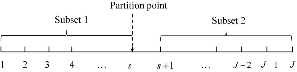
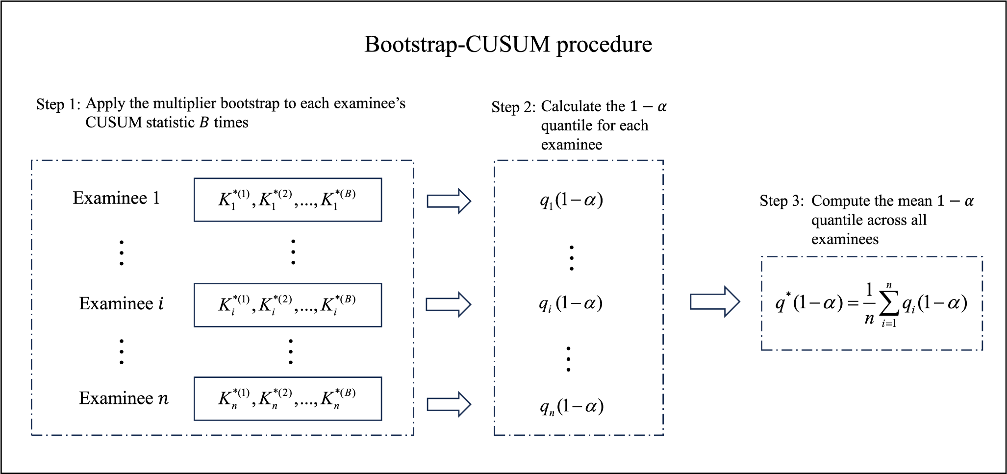
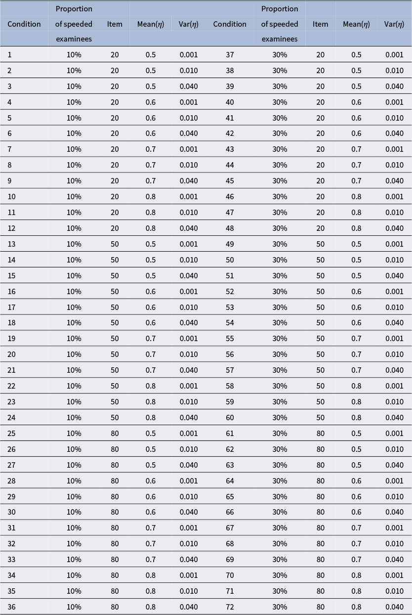

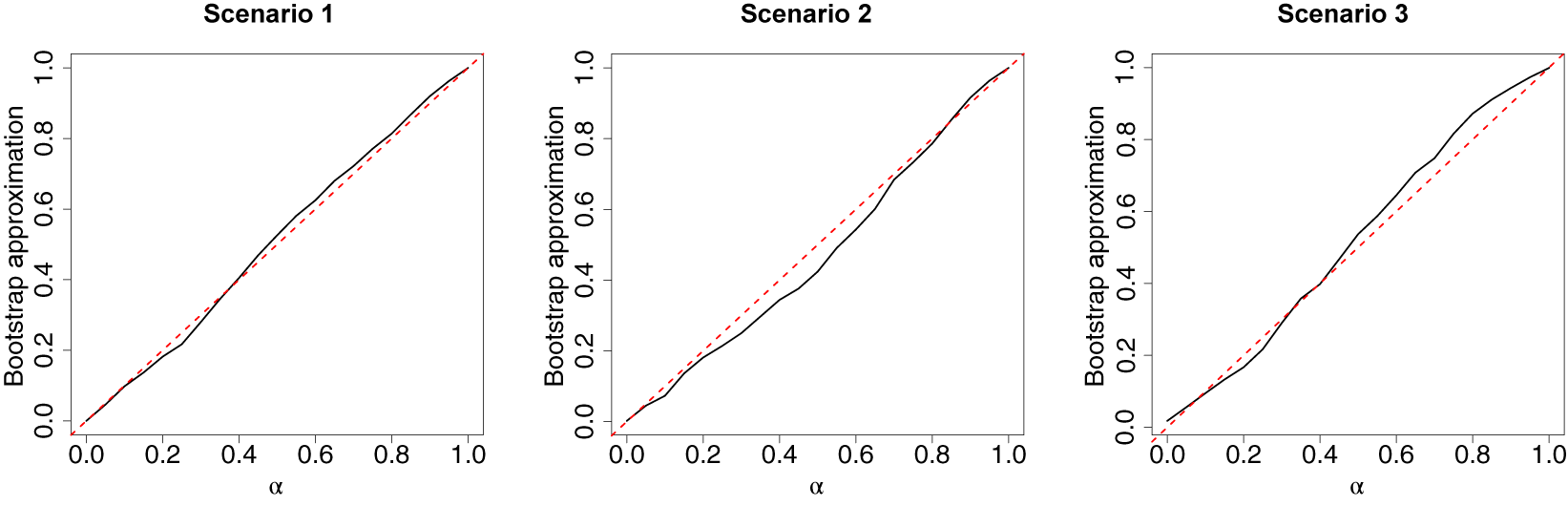


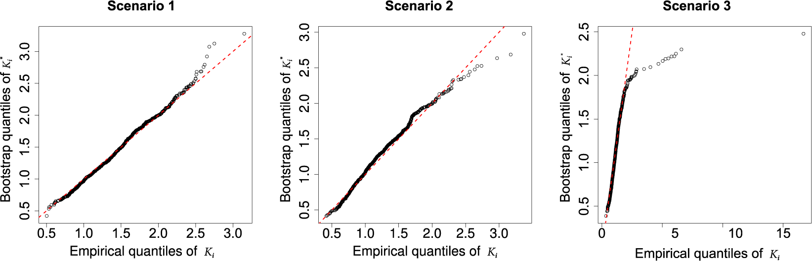


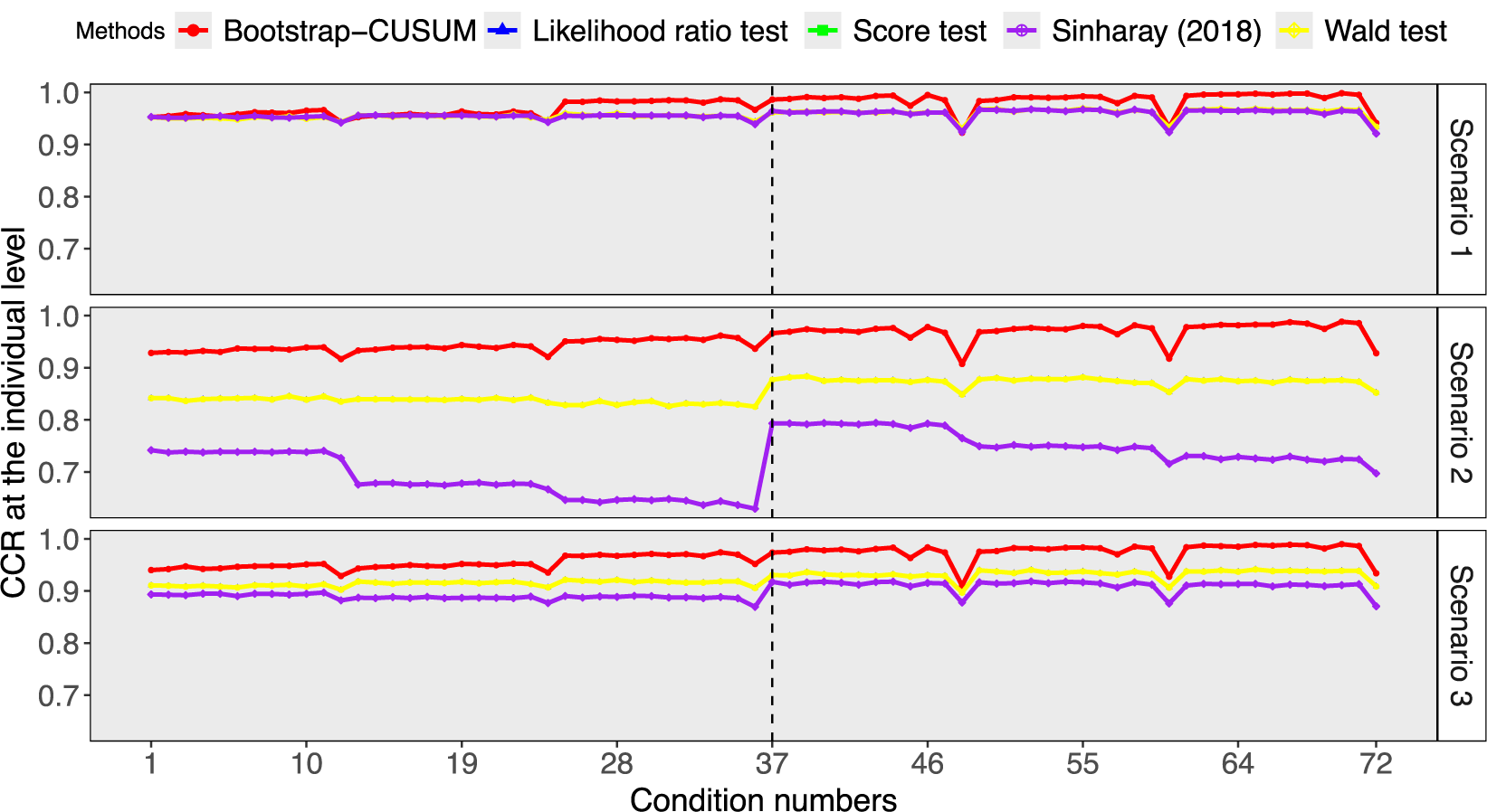


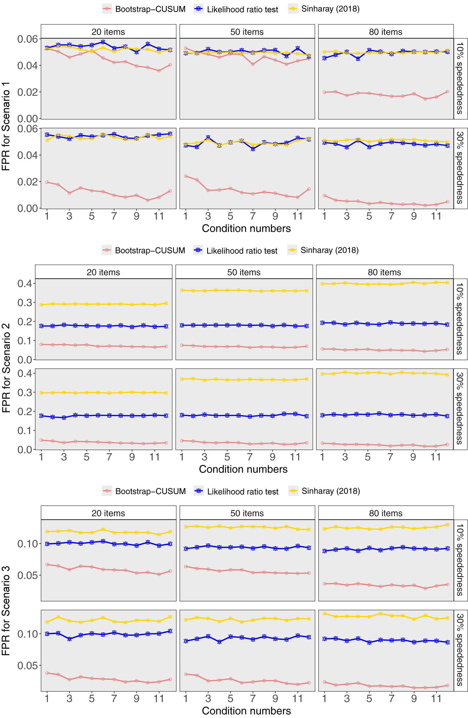
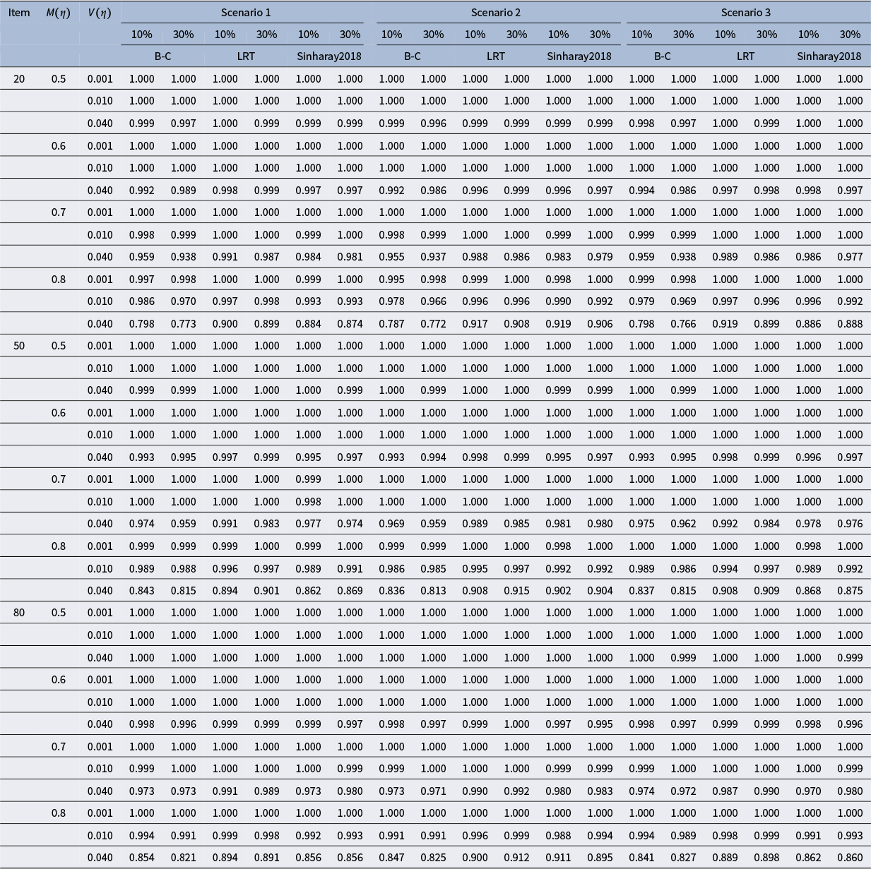
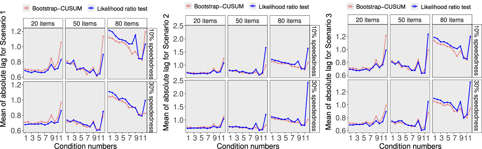
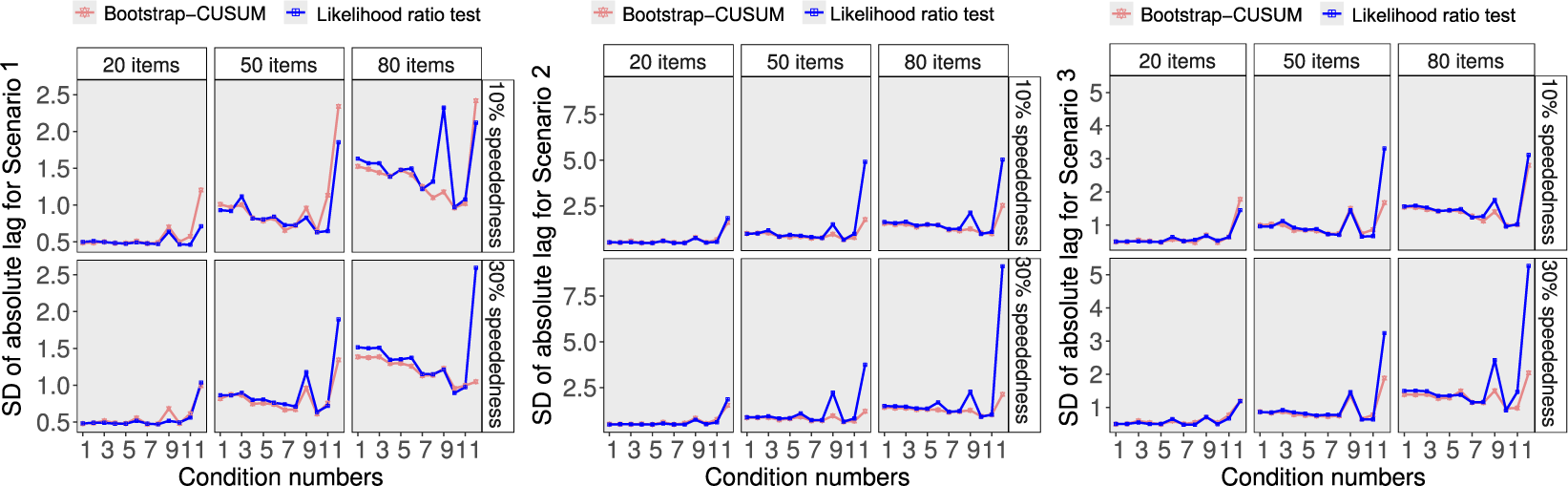
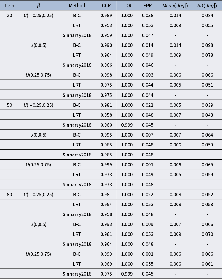
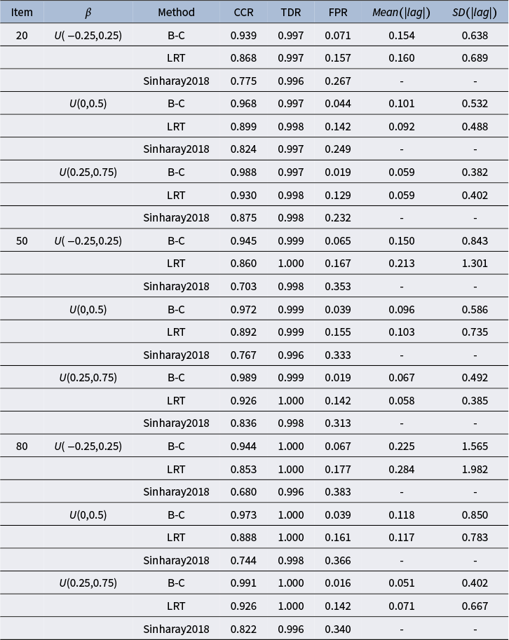
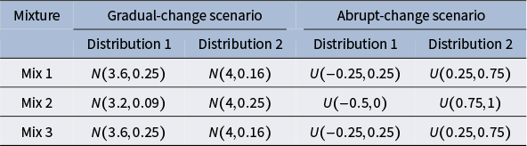

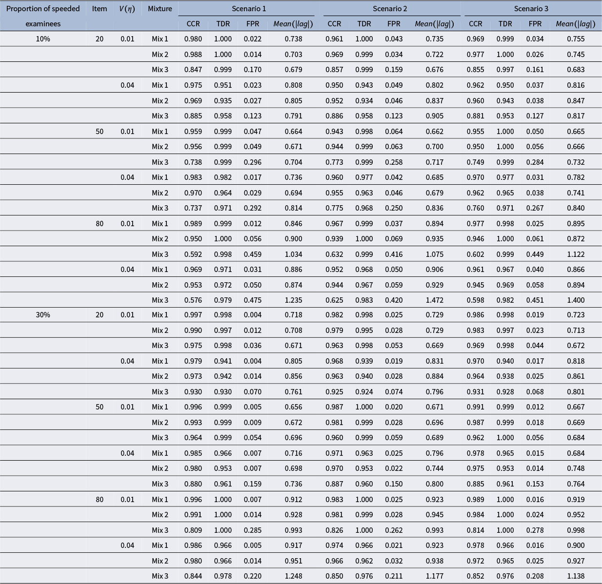
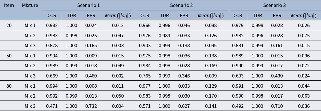
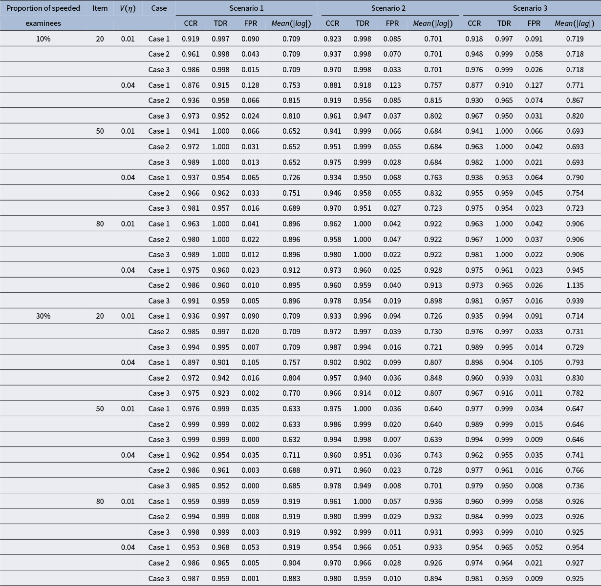
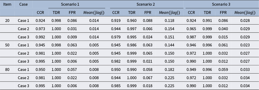
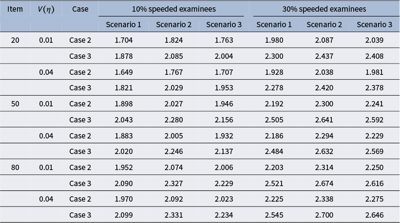
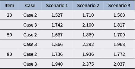
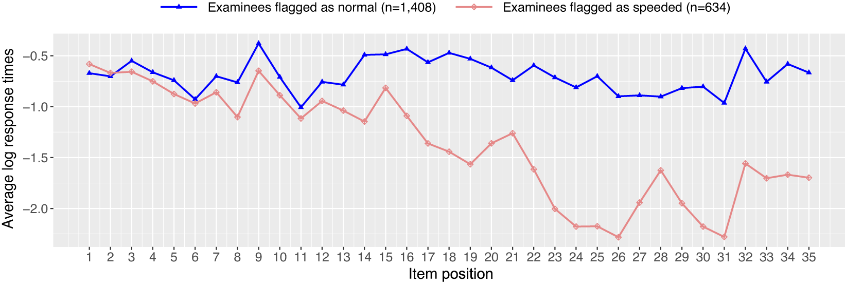
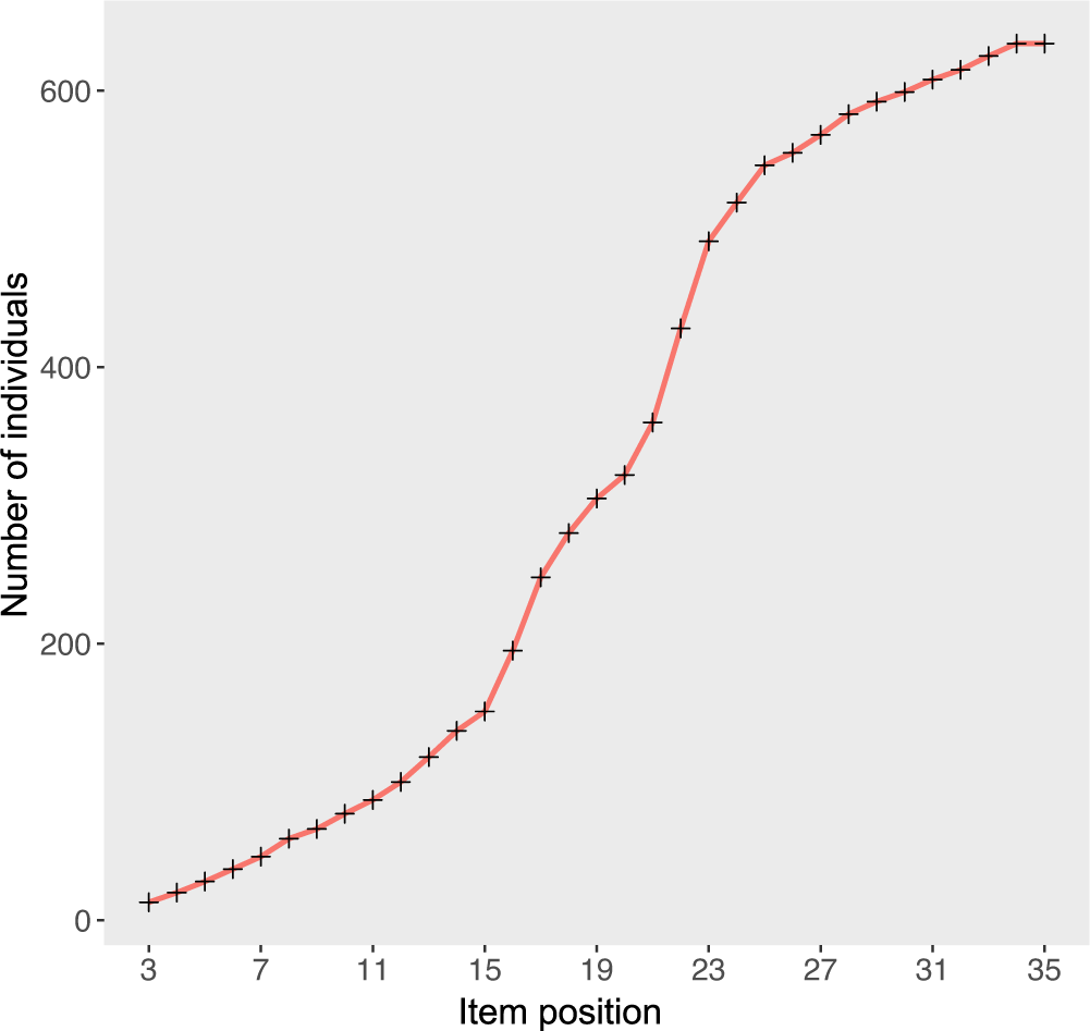
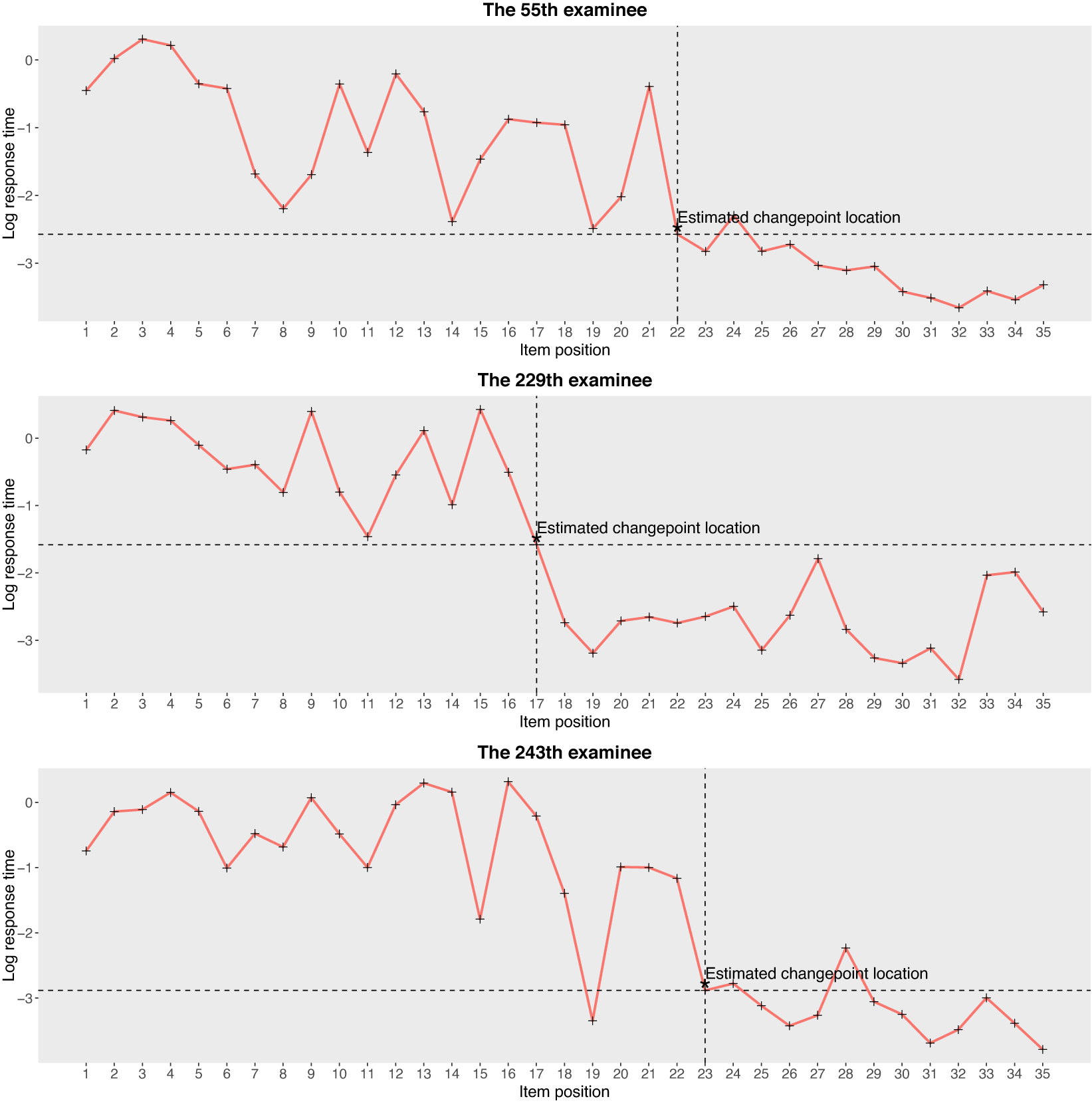


 Open access

