


1. Introduction
Over the past decades, glacial shrinkage and permafrost warming have been identified as drivers for the physical and socio-economical changes observed in high mountain areas. Numerous geomorphological processes acting on landscape dynamics are indeed related to changes in the mechanical stability of recently deglaciated rockwalls/slopes (Deline and others, Reference Deline, Gardent, Magnin and Ravanel2012, Reference Deline, Shroder, Haeberli and Whiteman2015; McColl, Reference McColl2012; Ravanel and others, Reference Ravanel, Deline, Lambiel and Vincent2013). Among them, the greatest sensitivity of deglaciated rock masses to variations in hydrological and thermal stresses is a well-documented preparatory and triggering mechanism for paraglacial rock mass failure (Ballantyne, Reference Ballantyne2002; Mercier and Etienne, Reference Mercier and Etienne2008; Slaymaker, Reference Slaymaker2009). In the latter, fatigue of the rock mass, driven by long-term addition of diurnal to seasonal stress modifications, is the main driver for fracture development and growth (Krautblatter and Leith, Reference Krautblatter and Leith2015; McColl and Draebing, Reference McColl, Draebing, Heckmann and Morche2019). For example, climate change-related permafrost warming has been documented as a preparatory and triggering phenomenon for an increasing number of high mountain rock mass failures (Gruber and others, Reference Gruber, Hoelzle and Haeberli2004; Fischer and others, Reference Fischer, Kääb, Huggel and Noetzli2006; Gruber and Haeberli, Reference Gruber and Haeberli2007; Caplan-Auerbach and others, Reference Caplan-Auerbach, Gruber, Molnia, Huggel and Wessels2008; Gruber, Reference Gruber2012; Deline and others, Reference Deline, Shroder, Haeberli and Whiteman2015; Ravanel and others, Reference Ravanel, Magnin and Deline2017; Duvillard and others, Reference Duvillard, Ravanel, Marcer and Schoeneich2019). The continued glacial shrinkage (Beniston and others, Reference Beniston2018; Jouvet and Huss, Reference Jouvet and Huss2019; Zekollari and others, Reference Zekollari, Huss and Farinotti2019), rising of the snowline elevation (Gobiet and others, Reference Gobiet2014; Radić and others, Reference Radić2014), reduction in frost frequency (Pohl and others, Reference Pohl2019) and overall snowfall (Klein and others, Reference Klein, Vitasse, Rixen, Marty and Rebetez2016) expected in the near future spark concern over the integrity of high mountain cryospheric bodies, and the stability of the underlying rockwalls (Krautblatter and others, Reference Krautblatter2010; Kenner and others, Reference Kenner2011; Stoffel and Huggel, Reference Stoffel and Huggel2012; Deline and others, Reference Deline, Shroder, Haeberli and Whiteman2015; Phillips and others, Reference Phillips2017).
While considerable efforts have been deployed to document and model the conditions leading to high mountain cryosphere-related failures (avalanching glaciers and permafrost; see Pralong and Funk, Reference Pralong and Funk2006; Huggel, Reference Huggel2009; Hasler, Reference Hasler2011; Faillettaz and others, Reference Faillettaz, Funk and Vincent2015; Krautblatter and Leith, Reference Krautblatter and Leith2015), very few studies have focused on the ice of currently deglaciating rockwalls. Ice-covered rockfaces have received hardly any attention but are likely undergoing drastic changes in thermal and mechanical conditions as the ice cover disappears. To our knowledge, only the studies of Galibert (Reference Galibert1960, Reference Galibert1964) provided qualitative descriptions of steep and thin ice covering high mountain rockfaces. As part of the mountain cryosphere, ice aprons are thought to have a negligible impact on sea-level rise and water resource availability. Nonetheless, as small-sized ice bodies, ice aprons are likely to be reliable indicators of climate change (Kuhn, Reference Kuhn1995; Dyurgerov and Meier, Reference Dyurgerov and Meier2000; Huss and Fischer, Reference Huss and Fischer2016) and to locally affect the stability of rockwalls (Kenner and others, Reference Kenner2011). Furthermore, ice aprons are mandatory passing points for numerous mountaineering routes (Mourey and others, Reference Mourey, Marcuzzi, Ravanel and Pallandre2019). Their change with time and climate as well as their relationships with other cryospheric objects in their vicinity (glaciers and permafrost) are still poorly understood. Ice apron/climate interactions and their relation to high mountain rockwall deglaciation need to be further investigated.
Our paper first aims at quantifying variations in surface area of six ice aprons located in the Mont-Blanc massif (France) since the end of the latest Little Ice Age (LIA) Alpine glaciers highstand (i.e. ≈1850, Matthews and Briffa, Reference Matthews and Briffa2005). In a second step, we assess potential relationships between the studied ice aprons and ongoing climate change. Section 2 reviews existing ice apron definitions. In Section 3, we detail the different study sites before further describing materials and methods used to quantify past variations in surface area in Section 4. According to the reported variations in surface area and with regards to meteorological data, we analyze the relationships between the studied ice aprons and climate in Section 5. A summary of the paper is presented in Section 6.
2. Definition and terminology
The definition of ice apron is not straightforward. According to Armstrong and others (Reference Armstrong, Roberts and Swithinbank1969), Benn and Evans (Reference Benn and Evans2010) and Bhutiyani (Reference Bhutiyani, Singh, Singh and Haritashya2011), ice aprons represent ‘small accumulations of snow and ice masses that stick to the topography of the glacierized basin’ and are ‘usually found above the equilibrium line’. Conversely, Cogley and others (Reference Cogley2011) state that the term ‘ice apron’ is synonymous to ‘mountain apron glacier’ and defined as ‘a small glacier of irregular outline, elongate along slope, in mountainous terrain’. While the definitions proposed by Armstrong and others (Reference Armstrong, Roberts and Swithinbank1969), Benn and Evans (Reference Benn and Evans2010) and Bhutiyani (Reference Bhutiyani, Singh, Singh and Haritashya2011) imply low, if any, flow of the ice mass, Cogley and others (Reference Cogley2011) explicitly state the existence of a past or present active ice motion in ice aprons. These two conflicting definitions reflect the lack of consensus on how to define ice aprons and the knowledge gap existing over the dynamics of such ice masses.
In the present study, we use the term ice apron to define very small (typically smaller than 0.1 km2 in extent) ice bodies of irregular outline, lying on slopes >40°, regardless of whether they are thick enough to deform under their own weight. To qualify as an ice apron, an ice body must persist for at least two consecutive years. We do not use the widespread maximum extent threshold for very small glaciers of 0.5 km2 (see Leigh and others (Reference Leigh2019) for more details) as we believe ice aprons of such dimension are very unlikely. Nonetheless, we doubt the studied sites (see Sections 3 and 5 for more) to be representative of the spectrum of possible ice apron extent and do not exclude the possibility of ice aprons with greater dimensions in other mountain ranges. The chosen slope angle is a common threshold in the material sciences community. It corresponds to the upper boundary limit of the stability angle for granular material (see e.g. Perla, Reference Perla and Voight1978; Barabási and others, Reference Barabási, Albert and Schiffer1999). Our adopted definition for ice apron covers ice masses from different settings such as entirely glaciated rockfaces (e.g. north face of Obergabelhorn, Pennine Alps), isolated massive ice patches on rockwalls (e.g. north face of Mt. Alberta, Canadian Rocky Mountains) and any steep ice body lying over a glacial bergschrund (Mair and Kuhn, Reference Mair and Kuhn1994), among others. Our study sites typically fall within the latter two settings ( see Section 3).
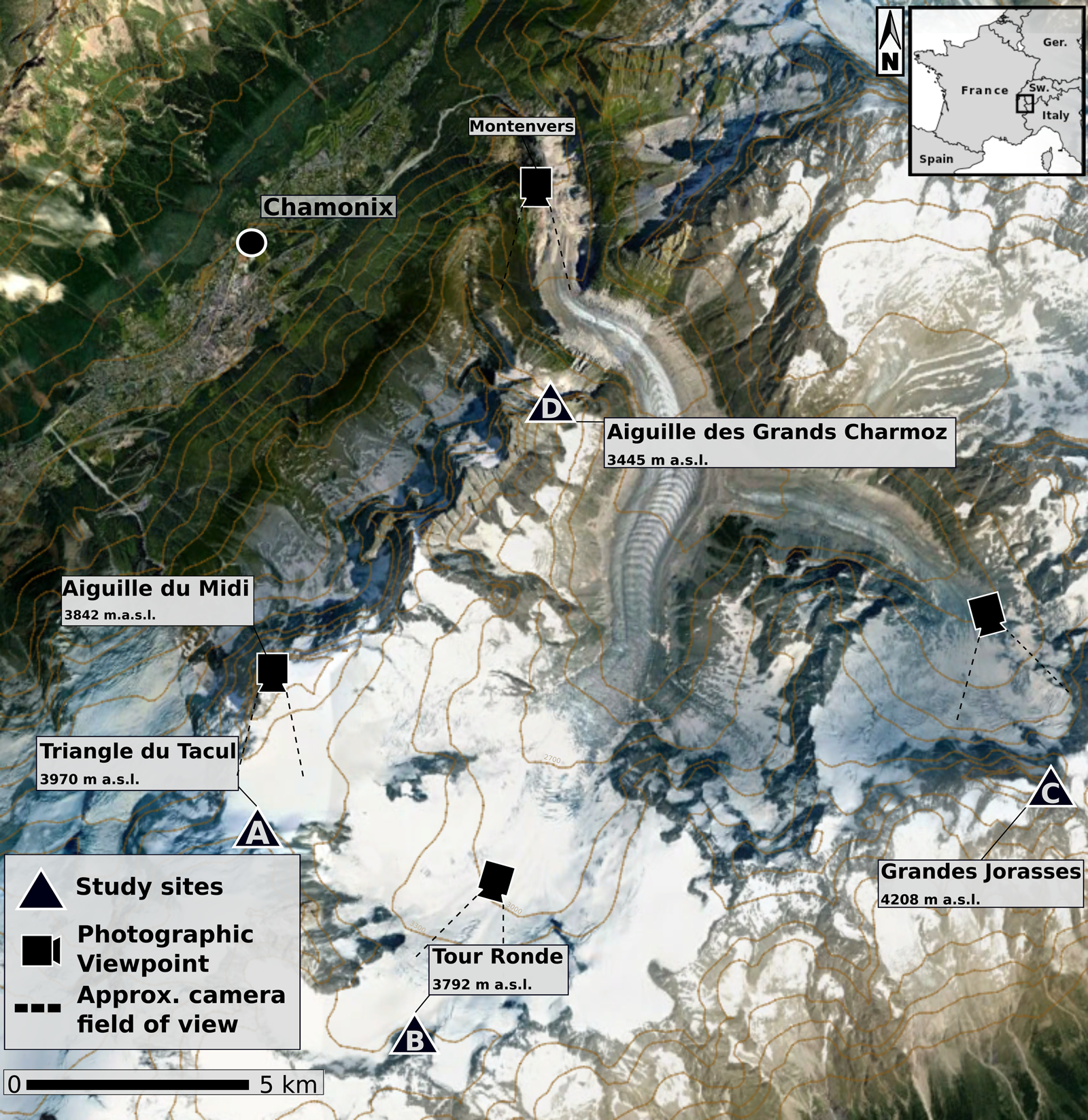
Localization map of the Mont Blanc massif and the study sites.
3. Study sites
The Mont Blanc massif forms the border between Italy, France and Switzerland. Spanning 550 km2, the Mont Blanc massif concentrates the highest peaks in the Western European Alps and displays very irregular terrain, with altitudes ranging from 581 m a.s.l. (town of Saint-Gervais-les-Bains) to 4809 m a.s.l. (summit of Mont Blanc). This terrain irregularity provides favorable conditions for the development of steep glacial bodies such as avalanching glaciers (Pralong and Funk, Reference Pralong and Funk2006) or ice aprons on north-facing bedrock slopes.
This study focuses on six ice aprons located on north-oriented steep rockwalls within the Mont Blanc massif (see Fig. 1):
(1) the north face of Triangle du Tacul (3970 m a.s.l.)
(2) the north face of Tour Ronde (3792 m a.s.l.)
(3) the north face of Grandes Jorasses (4208 m a.s.l.)
(4) the north face of Aiguille des Grands Charmoz (3445 m a.s.l.)
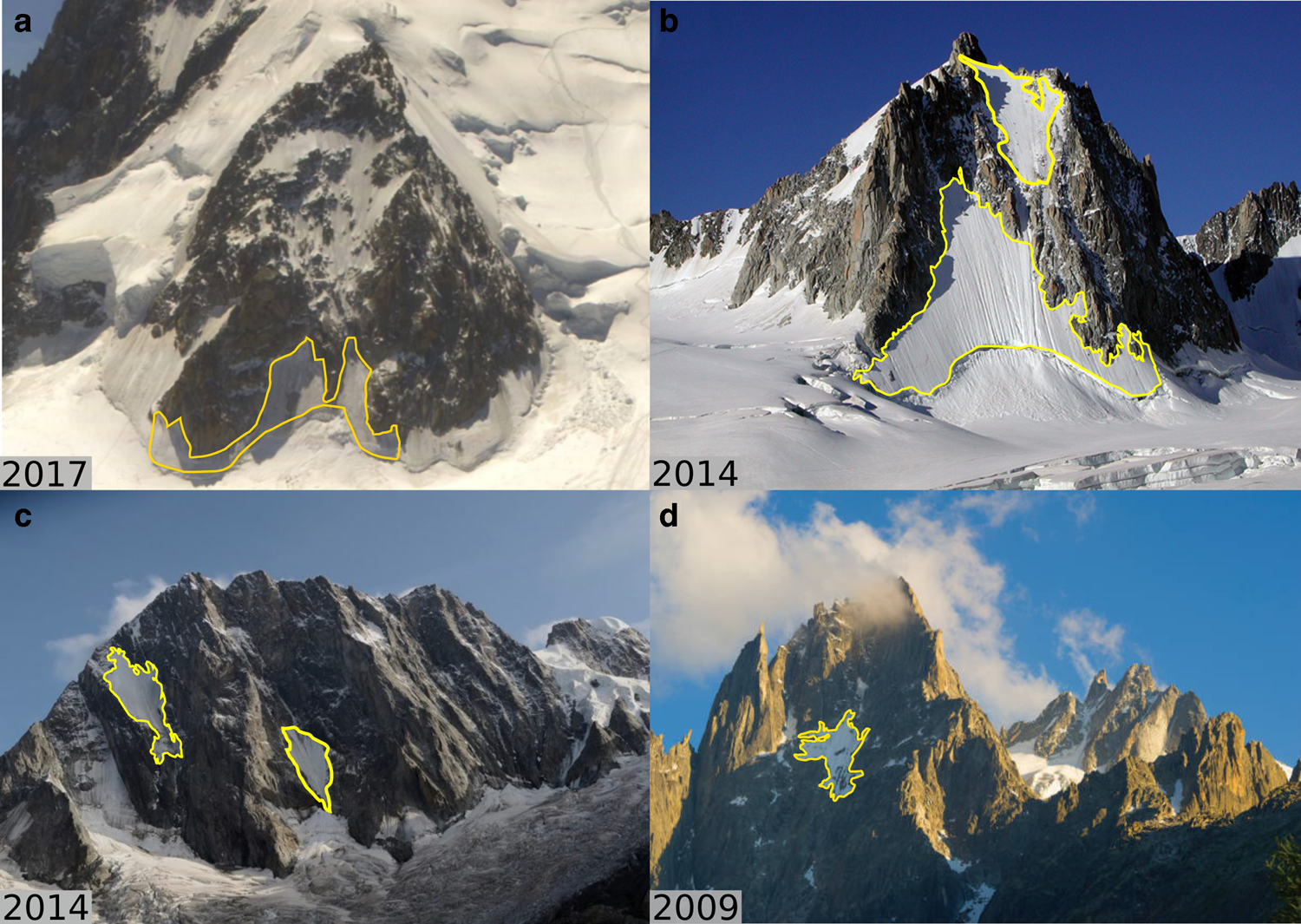
The studied ice aprons. Yellow outline represents the ice apron boundary. (a) Triangle du Tacul (3970 m a.s.l.). (b) Tour Ronde (3792 m a.s.l.). (c) Grandes Jorasses (4208 m a.s.l.). (d) Aiguille des Grands Charmoz (3445 m a.s.l.). None of these pictures were used to produce surface area estimates.
As our study relies heavily on the use of oblique historical imagery for extracting physical landscape measurements (see Section 4.1.1 for more details), the choice was made to select the most accessible ice aprons, as they are likely the best represented in mountain photography. The north faces of Grandes Jorasses and Aiguille des Grands Charmoz are easily observable from the Montenvers (Fig. 1), a panoramic viewpoint on the whole Mer-de-Glace basin, where the first hotel was opened in 1840 (Ballu, Reference Ballu2002). This broadens the studied time range as we were able to include photographs taken in the 1850s. The north faces of Triangle du Tacul and Tour Ronde are mainly documented since the 1950s, as the construction of the Aiguille du Midi cable-car enabled easy access to these remote sites. They have since become classical routes for mountaineers and are thus regularly documented.
The north face of Triangle du Tacul (Fig. 2a) lies in the accumulation zone of the Géant glacier. The mountain face is divided into two different ice aprons. We will hereafter focus on the lower one which extends from 3570 to 3690 m a.s.l. of elevation (0.004 km2 in 2018) and shows a mean slope of 59 ± 2°.
Similarly situated in the accumulation zone of the Géant glacier, Tour Ronde (Fig. 2b) forms the border between France and Italy. Its north face displays two ice aprons separated by a gully. The lower one, ranging from 3343 m a.s.l. at the bergschrund to 3594 m a.s.l. at its top (2015), will hereafter be called Lower Tour Ronde. The upper one, ranging from 3600 to 3750 m a.s.l. (2015), will be referred to as Upper Tour Ronde (0.005 km2 in 2012). Both ice aprons exhibit a mean slope of 55 ± 2°.
The north face of Grandes Jorasses (Fig. 2c), is a 1200 m-high rock face located in the Mont Mallet basin, in the accumulation zone of the eponymous glacier. Most of the rockwall, up to an elevation of 4000 m a.s.l., is covered by a 500 m-high and 170 m-wide ice apron (0.028 km2 in 2017). Overall, the Upper Grandes Jorasses ice apron displays a mean slope close to 63 ± 3°. The second studied ice apron located in the north face of Grandes Jorasses lies at the bottom of the face, between 3220 and 3650 m a.s.l., and will be further referred to as Lower Grandes Jorasses. Its average slope is similar to that of Upper Grandes Jorasses.
The north face of Aiguille des Grands Charmoz lies over the Mer-de-Glace basin (Fig. 2d). The ice apron lies between 2907 and 3185 m a.s.l. of elevation (2015). Contrary to the other studied ice aprons, the Grands Charmoz ice apron is not located within the accumulation zone of a large valley glacier. The ice apron shows a mean slope of ~52 ± 2°.
4. Materials and methods
In the present study, we estimate the evolution of surface area for six different ice aprons from photographs taken between 1854 and 2018. To this end, we rely on a photogrammetric inverse perspective method, presented in detail in Guillet and others (Reference Guillet, Guillet and Ravanel2020). This particular technique aims at extracting referenced landscape feature measurements from a single image by estimating the parameters of the imaging camera using ground control points (GCPs), such as peaks or noticeable buildings (e.g. Förstner and Wrobel, Reference Förstner and Wrobel2016). Extracted measurements are then back-projected onto a Digital Elevation Model (DEM), thus providing an estimate of the ice apron surface area. Similar methods have already been used to document and reconstruct changes in glacier states in the Himalayas (Byers, Reference Byers2007), the Swiss (Wiesmann and others, Reference Wiesmann2012) and Julian Alps (Triglav-Čekada and Gabrovec, Reference Triglav-Čekada and Gabrovec2013), among others.
In this section, we start by detailing the data used for this study (Section 4.1). We then briefly describe our inverse perspective method, which provides our surface area estimates and uncertainties (Section 4.2). We finally derive a model of surface area evolution based on meteorological data (Sections 4.3 and 4.4).
4.1 Data description
4.1.1 Photographs
This study relies on the joint use of terrestrial oblique photographs and aerial single images for extracting discrete ice apron surface area estimates. Working with single photographs allows one to tap into a wealth of available data readily accessible from the Internet such as aerial surveys, historical records or user-contributed photographs. Ice apron surface area estimates can hence be extracted from photographs taken with no prior scientific intention and in this instance allowing us to cover a 164-year time range.
For this study, we used photographs from diverse sources:
• Aerial photographs come from various photographic surveys carried out by the IGN (Institut Géographique National, French National Geographic Institute) and are publicly available (Institut Géographique National, 2019). Such photographs cover a time span of 64 years, from 1949 to 2012. The list of aerial photographs used in this study is provided in the Appendix.
• Terrestrial oblique photographs originate from private collections. Photographs originating from the 19th and 20th centuries were taken by professional photographers. Photographs taken after that period originate from the authors' and their relatives' private collections.
Seasonal variations in snow cover are likely to impact the estimated ice apron surface area. To ensure comparable estimates, we selected only photographs taken in late summer, and preferably, in September. All IGN aerial photographs provide accurate timestamps. Most recent terrestrial digital photographs provide date and time information, for example, in embedded EXIF metadata. For historical photographs, while generally only the year is known, the season in the year can easily be identified by the presence of seasonal snow at low- to mid-altitudes (winter and spring or fall), and we exclude any photograph shot in the winter or spring. Finally, all photographs taken in summer which show evidence of recent snowfall are rejected. In this process, we are typically looking for sparse snow patches on nearby rockfaces, and recent avalanche activity overlaying the bergschrunds. After the selection process, our final corpus is composed of a total of 55 photographs.
4.1.2 Digital elevation model
The DEM used is provided by a regional French agency (Régie de Gestion des Données des Pays de Savoie). It was constructed from 1998 aerial photographs, revised in 2004 through photogrammetric GCPs, and further updated in 2008 and 2010. The DEM is provided to us as rectilinear gridded data with 4 m node spacing (horizontal resolution) in both easting and northing, in the Lambert-93 projection. The documentation reports an estimated vertical root mean square error (RMSE) ranging from 1 m in plains to 4 m in rugged and alpine high altitude areas. The back-projection model accounts for errors in the DEM based on an RMSE comparable to published specifications; our uncertainty model accounts for spatially correlated vertical errors which can easily exceed 4 m in steep terrain (see Guillet and others (Reference Guillet, Guillet and Ravanel2020) for details). It should be noted that the DEM is likely to change in time, as a consequence of variations in ice apron volume. Considering the small dimensions of the studied objects, we assume such changes in the DEM to be in the same order of magnitude as the DEM resolution.
4.1.3 Ground control points
We manually determine 2D/3D control point matches. We proceed by identifying well-defined features on the photograph, such as road crossings, mountain peaks, corners of noticeable buildings, and match them to their known position in 3D world coordinates. 3D world positions are determined by detailed topographical maps and completed, if needed, with planimetric and altimetric databases such as OpenStreetMap (OpenStreetMap contributors, 2019). As 3D GCPs coordinates do not come from high-precision geodetic surveys, their typical accuracy is of the order of a few meters.
4.2 From single photographs to ice apron surface area: camera calibration and inverse perspective with uncertainties
For this study, we use the Bayesian framework developed in Guillet and others (Reference Guillet, Guillet and Ravanel2020) to reconstruct the surface areas and their uncertainties from individual photographs.
In photogrammetric applications, measurements are usually extracted from single photographs using camera models with known camera parameters. In our study, photographs come from various sources; for most photographs, the camera parameters and the imaging system used are unknown. It is therefore necessary to compute an estimate of the camera parameters used to take each picture.
This process, called camera calibration, aims at finding a set of admissible camera parameters that can reproduce the observed 2D control points by projection of the 3D points, given a chosen camera projection model (Fig. 3). Once the camera is calibrated, the outline of the ice apron is manually traced on the picture as a polygon. Using the estimated camera parameters, we finally invert the perspective of the calibrated camera and project the 2D polygon onto the DEM.
Overview of the inverse perspective problem. 2D control points (blue) are defined on the picture and matched with their corresponding 3D world coordinates (red). The matches are used to estimate the parameters of the imaging camera. The 2D polygon (blue) is then backprojected onto the DEM in order to obtain the surface area estimate (red). Shaded areas typically illustrate the uncertainties on true location (see text for further details). Modified from Guillet and others (Reference Guillet, Guillet and Ravanel2020).

There are four main sources of uncertainties that we account for in our reconstruction of the surface area:
(1) Finding the 2D location of a control point on the image involves some level of uncertainty. The accuracy of 2D point picking depends on several factors such as image resolution, blurriness, contrast or perspective among others. For low-resolution imagery, we can expect uncertainties of <5 pixels, while high-resolution aerial pictures typically allow for lower GCP location uncertainties, typically between 1 and 2 pixels.
(2) The positions of the GCPs in 3D world coordinates are known up to a certain level of accuracy. The uncertainty over the true 3D GCP location varies with surveying method. While GPS-surveyed GCPs could be located with centimetric accuracy, coordinates derived from maps typically only provide an accuracy of a few meters, at best.
(3) Similarly to 2D GCPs, the manual polygon tracing step introduces systematic errors originating from the precision with which ice apron margins can be identified.
(4) Finally, errors arise from the accuracy of the DEM itself.
The method proposed in Guillet and others (Reference Guillet, Guillet and Ravanel2020) allows one to compute the camera parameters as a probability distribution of admissible camera parameters, rather than a single value estimate. From the probability distribution on camera parameters, a number N of samples is randomly drawn. Each of the samples is then used to back-project the polygon onto the DEM. Here, we typically use N = 5000. For each photograph, the extracted ice apron surface area thus corresponds to a probability distribution, originating from 5000 different back-projections of the polygon.
4.3 Meteorological data
In our study, our goal is to correlate variations in surface area estimates with accumulation and ablation proxies. For our study sites, the closest permanent weather station is the MeteoFrance Aiguille du Midi station (3842 m a.s.l., abbreviated AdM, see Fig. 1). However, no precipitation records are available for the AdM station. We thus consider monthly temperature and precipitation records from the Col du Grand-Saint-Bernard (2469 m a.s.l., abbreviated GSB) weather station (MeteoSwiss), over the 1860–2018 period. Located 15 km eastward from Grandes Jorasses (4208 m a.s.l.) and Aiguille du Midi, the Col du Grand-Saint-Bernard presents a similar climatological regime.
With the aim of modeling the monthly averaged temperature at elevations closer to our study sites, we study the correlation between AdM and GSB datasets. Because of the strong correlation between monthly averaged AdM and GSB temperature records (Pearson'sr = 0.98, p-value < 0.001, see Fig. 4), we model the monthly averaged AdM temperature from the GSB temperature using a linear model:

where a = 0.87, b = −7.7°C, r are, respectively, the slope, intercept and residuals with zero mean.
Correlation (Pearson's r = 0.98, p < 0.001) between the monthly averaged temperature measurements at the Aiguille du Midi (AdM) and the Col du Grand Saint Bernard (GSB) for the 2007–2018 period.

From the AdM data reconstructed using 1, we estimate an annual sum of positive degree-days (PDD), using the method proposed by Calov and Greve (Reference Calov and Greve2005). This method, based on the ideas of Reeh (Reference Reeh1991) and Braithwaite (Reference Braithwaite1995), proposes a probabilistic approach to the computation of the PDD. The annual sum of PDD is thus computed from the normal probability distribution centered on the mean monthly temperature. Calov and Greve (Reference Calov and Greve2005) also account for stochastic variations in temperature in the computation of the PDD. We then calculate the cumulative PDD and use it as a proxy for ablation (Braithwaite and Olesen, Reference Braithwaite, Olesen and Oerlemans1989; Vincent and Vallon, Reference Vincent and Vallon1997).
Accumulation is approximated as the yearly sum of precipitation occurring at a temperature between −5 and 0°C, as only snowfall within this temperature range is believed to accumulate in steep terrain (Kuroiwa and others, Reference Kuroiwa, Mizuno and Takeuchi1967). Other local mass-balance drivers such as wind redistribution and erosion, gravitational transport and probable feedback – positive or negative – between surface slope variations and accumulation or ablation, among others, are neglected.
4.4 Surface area model
We finally derive the surface area model for the studied ice aprons. We propose to model the differences between surface area measurements at different time steps, as the result of time-integrated changes in climatic forcing. Here, we are typically looking for a potential linear relationship between variations in ice apron surface area and the defined climate forcing by using a multivariate regression model. More formally, it can be written as follows:

where S m(t) corresponds to the modeled surface area at time t. Similarly, CPDD(t)and A(t) represent our proxies for ablation and accumulation. S(t = 0) is the first measurement available for each individual ice apron. α 1 and α 2 are the coefficients of linear regression, β is the intercept, and ε the residuals. χ(T, t) accounts for precipitation occurring in the [ − 5°C, 0°C] temperature range. It is written as the temperature-dependent indicator function of the form:

5. Results and discussion
In this section, we first present the time series of surface area estimates. We then review the potential correlation between extracted and modeled ice apron surface areas. Finally, we discuss the sensitivity of the studied ice aprons to small-scale processes and local mass-balance drivers.
5.1 Changes in ice apron extent: the decrease in surface area
Time series of surface area estimates are presented in Figure 5, and summarized in Table 1. The studied sites show similar trends in surface area evolution, with details varying between individual ice aprons. Despite significant data gaps, results indicate that the largest ice aprons expansion occurs at the end of the 19th century. We observe a decrease in relative surface area from the beginning of the 20th century to the end of the 1960s. The Grands Charmoz ice apron shows the most substantial surface loss, decreasing 40% (≈−13000 m2) between 1900 and 1966. Lower Tour Ronde and Lower Grandes Jorasses exhibit similar trends, with a relative surface area loss ~30% (≈−6100 m2) for the 1880–1966 period. Relative surface losses are lower for the Triangle du Tacul and Upper Grandes Jorasses ice aprons, with 18% (≈770 m2) and 13% (≈−5000 m2) observed shrinkage, respectively. Overall decrease (1850s to late 1960s) is followed by a period of ~20 years of expansion, reaching its maximum by the end of the 1980s for the Grands Charmoz, Tour Ronde (upper and lower) and Triangle du Tacul ice aprons. In 1988, the Upper Grandes Jorasses ice apron attains a surface area close to its 1854 extent. Between 1988 and 1993, we observe an important decrease in the Grands Charmoz and Upper Tour Ronde time series. The ice apron was fragmented in smaller ice bodies as the steepest parts of the ice apron are separated from the underlying main body (Fig. 6). Since the 1990s, shrinkage is observed over all the investigated ice aprons.
Evolution of surface area for the six studied ice aprons of the Mont Blanc massif. Error bars represent the 90% confidence interval obtained from the polygon back projection process.

Evolution of the Grand Charmoz ice apron between 1989 and 2017. Between 1989 and 1993, the lower part of the ice apron (blue) is fragmented from the two ice gullies (red). As often observed, the ice apron is successively fragmented in smaller ice bodies before total melt in 2017.

Summary of the variations of surface area for the six study sites. S(t)/S(t0) represents normalization of the surface area measurement at time t by the first estimate

Both Lower Tour Ronde and Triangle du Tacul exhibit an average shrinking rate in surface area of 1%a−1 between 1984 and 2018. Over the same period, the decrease for Upper Grandes Jorasses is close to 0.7%a−1. Again, the Lower Grandes Jorasses, Upper Tour Ronde and Grands Charmoz ice aprons record the highest decrease rates, with2.6%a−1, 3.6%a−1 and 4.8%a−1, respectively. Ice apron shrinkage from the 19th and 20th centuries to 2018 is further illustrated in Figure 7.
Comparison of photographs for: (a) Triangle du Tacul (upper and lower), (b) Tour Ronde (upper and lower) and (c) Grandes Jorasses. Yellow dashed line represents ice apron outlines from the left picture. The steepest sections of the ice aprons are the first parts to display shrinkage. Note that the presented Tour Ronde pictures were not used to extract surface area measurement of the Upper Tour Ronde ice apron hence, the black outline of Upper Tour Ronde (b) is a crude representation of 1880 ice apron extent.

Overall, our records of surface area and of their estimated shrinking rates of a total of ~90 000 m2 over the period 1854–2018 are consistent with previous results from similar studies (Hoffman and others, Reference Hoffman, Fountain and Achuff2007; Andreassen and others, Reference Andreassen, Paul, Kääb and Hausberg2008; Bolch and others, Reference Bolch, Pieczonka and Benn2011; Serrano and others, Reference Serrano, González-trueba, Sanjosé and Del río2011; Shahgedanova and others, Reference Shahgedanova, Nosenko, Bushueva and Ivanov2012; Marti and others, Reference Marti2015; Zemp and others, Reference Zemp2015).
5.2 Climate change as a driver for ice apron shrinkage
Figure 8 illustrates the correlation between measured and modeled normalized surface area estimates for all the studied ice aprons. We observe a strong linear correlation (Pearson's r = 0.92, p-value = 0.001) between the mean normalized surface area estimates extracted from the photographs and the modeled normalized surface areas (Fig. 8). The best-fitting line presents a slope of 1.0 and an intercept of 0.0. These results demonstrate the proficiency of the proposed surface area model in computing new ice apron states from the accumulation and ablation proxies. It is, however, important to note that we observe substantial scatter in the data, with a std dev. of 0.23.
Correlation between the mean normalized surface area estimates and the modeled surface areas. S(t)/S(t0) represents normalization of the surface area measurement at time t by the first estimate. Similarly, S m(t)/S(t 0) represents normalization of the modeled surface area at time t. The dashed lines represent the best fit line of equation y = x (see text for further details).

We will now review site-specific ice apron/climate relationships for each individual ice apron. Table 2 summarizes regression parameters and correlation metrics for each study site. Figure 9 illustrates the correlation between measured and modeled normalized surface area estimates for each independent ice apron. As before, we observed linear relationships between modeled and extracted surface areas. Our results however show discrepancies between the different ice aprons. The most notable one is the Upper Grandes Jorasses ice apron for which the linear relationship is the weakest (Table 2). Due to their small dimensions, all the studied ice aprons do not display standard accumulation and ablation zones. Mass gain and loss mainly occur across the ice apron in its entirety, with a major impact near the ice margins (Fig. 7). No evidence of ice flow at the surface could be observed between photographs. The latter suggests that downward mass transfer has very small, if any, impact on the ice aprons and that such ice masses should respond rapidly to climate change (Kuhn, Reference Kuhn1995). A simple approach to modeling surface area variations, based exclusively on PDD and precipitation as proxies for ablation and accumulation, appears suitable for the study of ice aprons over several study sites. However, the proposed model failed to constrain site-specific surface area variations, especially for the Upper Grandes Jorasses ice apron.
Correlation between the mean normalized surface area estimates and the modeled surface areas for each individual study site. Shaded areas represent 95% confidence interval of the linear fit. S(t)/S(t 0) represents normalization of the surface area measurement at time t by the first estimate. Similarly, S m(t)/S(t 0) represents similar normalization of the modeled surface area at time t. Pearson's correlation coefficient and other regression metrics are further detailed in Table 2.

Linear regression parameters and correlation metrics for each individual study site

5.3 The importance of local mass-balance drivers
Discrepancies in surface area evolution between individual ice aprons can primarily be related to elevation differences. The works of Hantel and others (Reference Hantel, Maurer and Mayer2012) documented the median summer snowline (snow probability 0.50) of the Alps 1961–2010 to be 3083 ± 121 m a.s.l. Similarly, Rabatel and others (Reference Rabatel, Letréguilly, Dedieu and Eckert2013) proposed a regional equilibrium line altitude (ELA) of 3035 ± 120 m a.s.l. for the western Alps (1984–2010). As mentioned above, ice aprons do not display standard accumulation and ablation zones. ELA approaches are therefore not well-suited to study the mass balance of ice aprons. Nonetheless, in the present case, both the ELA and the snowline are mentioned as reference altitudes at which we are to expect conservation of snow cover during summer. With altitudes ranging from 2900 to 3200 m a.s.l., a substantial part of the Grand Charmoz ice apron lies below the ELA and the snowline. In addition, Rabatel and others (Reference Rabatel, Letréguilly, Dedieu and Eckert2013) describe rising of the ELA to 3250 ± 135 m a.s.l. during the 2003 heat wave, bringing the ELA higher than the upper margin of the ice apron (3200 m a.s.l.). Similar scenarios likely happened during the subsequent heat waves of 2006, 2015 and 2017 (Della-Marta and others, Reference Della-Marta, Haylock, Luterbacher and Wanner2007; Hoy and others, Reference Hoy, Hänsel, Skalak, Ustrnul and Bochníček2017), leading to complete melting of the Grands Charmoz ice apron in August 2017 (Fig. 6).
Differences in elevation between ice aprons cannot however explain the rates of yearly loss recorded by the Lower Grandes Jorasses and Upper Tour Ronde ice aprons since the end of the 1990s. Hoffman and others (Reference Hoffman, Fountain and Achuff2007) and DeBeer and Sharp (Reference DeBeer and Sharp2009), among others, demonstrated the importance of accounting for local mass-balance drivers in variations of ice masses. Local topography is a documented factor contributing to the persistence of small glaciers lying under the regional ELA (Florentine and others, Reference Florentine, Harper, Fagre, Moore and Peitzsch2018). Here, we suggest that local topography mitigates ice apron persistence, especially for Lower Grandes Jorasses and Upper Tour Ronde. Figure 7 shows that for these two ice aprons, most of the recorded loss occurs on a topographical ridge. Ridge-like topographies lead to unobstructed surfaces and introduce local changes in slope aspect, altering the energy balance of ice masses lying on the ridge (Gratton and others, Reference Gratton, Howarth and Marceau1993; Evans, Reference Evans2006). Furthermore, it can be inferred that thermal radiation emitted from recently deglaciated zones will further accelerate the melt of nearby ice aprons (Paul and others, Reference Paul, Kääb, Maisch, Kellenberger and Haeberli2004). It is also worth noting that the Upper Tour Ronde ice apron lies on the summit ridge; therefore, we believe that summer horizontal (south to north) heat fluxes likely affect the energy balance of the summital part of Upper Tour Ronde ice apron (Noetzli and others, Reference Noetzli, Gruber, Kohl, Salzmann and Haeberli2007). We further suggest that the steepness of the studied ice aprons is severely limiting accumulation. In this type of complex topography, avalanching will scour snow away from the ice apron, exposing the bare ice and the same is to be expected from wind, which can relocate or sublimate snow (Vionnet and others, Reference Vionnet2014).
Several studies discussed the need to account for decadal variations in radiation (secondary to changes in cloudiness or solar dimming/brightening) in mass-balance modeling (Gerbaux and others, Reference Gerbaux, Genthon, Etchevers, Vincent and Dedieu2005; Huss and others, Reference Huss, Funk and Ohmura2009; Thibert and others, Reference Thibert, Dkengne Sielenou, Vionnet, Eckert and Vincent2018). Here, we chose to use a simple temperature-index model as a first approach to simulate surface area variations of the studied ice aprons (Reveillet and others, Reference Reveillet, Vincent, Six and Rabatel2017). While our results demonstrate the importance of air temperature and precipitation on the observed surface area variations, we expect global radiation to play a role in the mass and energy balance of ice aprons. Clarifying the sensitivity of ice aprons to long-term changes in global radiation is of importance to allow meaningful projections of ice aprons evolution during the 21st century, and should be addressed in future studies.
Our results show that ice aprons react rapidly to changes in climate forcing (see Figs 8, 9 and Table 2). Most local mass-balance drivers mitigate the accumulation of snow and thus enhance the impact of air temperature on ice aprons. This poses the question of the sensitivity of ice aprons to extreme weather events. Given the sampling rate of our surface area measurements, it is not possible to quantify the contribution of individual extreme weather events, such as the 2003 heat wave. Yet, we believe that heat waves occurring when the ice apron is free of snow (in winter and midsummer) will have the greatest effect. With regards to the foreseeable increase in intensity, frequency and length of heat waves in the 21st century (Meehl and Tebaldi, Reference Meehl and Tebaldi2004), there is a pressing need for a better understanding of ice apron sensitivity to extreme weather events.
6. Conclusions and outlooks
In this paper, we presented time series of surface area estimates for six ice aprons located in the Mont Blanc massif over the period 1854–2018 using 55 terrestrial and aerial oblique photographs to produce estimates of end-of-summer surface area (Table 1).
The studied ice aprons shrank between the end of 1850s and the mid- to late-1960s. While a short period of ice apron expansion occurred from the early 1970s to the early 1990s, we observe an accelerated recession of all ice aprons since the beginning of the 21st century. Over the studied time period (e.g. 1850s–2018), the Upper Grandes Jorasses display shrinkage ~20% (−7400 ± 200 m2, see Table 1) while the Triangle du Tacul, Upper Tour Ronde and Lower Tour Ronde ice aprons lost 35% (−1940 ± 158 m2), 40% (−3500 ± 147 m2) and 50% (−1100 ± 127 m2, see Fig. 5 and Table 1). The Lower Grandes Jorasses ice apron exhibits shrinkage ~60% (−28440 ± 550 m2, see Fig. 5 and Table 1). The most dramatic example of ice apron shrinkage is the Grands Charmoz ice apron which melted completely during the summer of 2017.
In parallel, we derived an ice apron surface area model based on meteorological data. We used the precipitation record, focusing on snowfall occurring between −5 and 0°C, and a simple PDD approach, as proxies for accumulation and ablation, respectively. Combining time-integrated accumulation with a temperature-index, the model consistently estimated variations in ice apron surface area. Applied to our sites of interest, our study showed discrepancies in surface area variations between individual ice aprons. While discrepancies in surface area variations could primarily be related to differences in elevation, we also noted the importance of local topography on both the energy and mass balances of ice aprons.
Ice aprons stand out as an important component of the high-alpine cryospheric system; given the observed shrinking rates and existing climate scenarios, severe concerns exist over the fate of the studied ice aprons. Climate change-related modifications in ice aprons are likely to alter the whole high mountain environment; most notably, the loss of ice aprons is thought to have major consequences over the mechanical and thermodynamical stability of the underlying steep rockfaces. We believe the impact of ice apron loss over the underlying steep high mountain rockwalls needs to be further addressed.
Acknowledgements
This study is part of the ANR 14-CE03-0006 VIP Mont Blanc and the ALCOTRA n342 PrevRisk Haute Montagne projects. We thank the editor and two anonymous reviewers for their constructive remarks on the manuscript.
Appendix
Table of aerial IGN photographs used in this study

Table of terrestrial oblique photographs used in this study


 Open access