


1. Introduction
Fairness in networked systems is often defined using population-level statistics, while individuals experience and evaluate fairness through local social comparisons. In many social, economic, and algorithmic contexts, agents observe only the outcomes of their neighbors and infer fairness from this limited information. As a result, perceived fairness may differ substantially from objective fairness defined at the population level.
Network structure plays a central role in this discrepancy. Homophily, degree heterogeneity, and clustering shape who observes whom and therefore how outcomes are locally compared. Even when a decision rule satisfies standard fairness criteria globally, network topology may distort local exposure and generate systematic differences in perceived fairness across groups.
This paper develops a concise analytical framework to study perceived fairness on networks. We model perceived fairness as a local comparison between an individual’s outcome (or acceptance probability) and the average outcome observed in their network neighborhood. We then analyze how topological features affect the gap between objective and perceived fairness.
Our results show that perceived fairness converges to objective fairness only when individuals observe the entire population. At finite visibility, homophily and degree heterogeneity amplify perceived discrimination, while clustering mitigates dispersion by stabilizing local averages. These effects are structural and arise independently of any intentional bias in the decision rule.
1.1 Contributions
The paper makes four main contributions: (i) it formalizes perceived fairness as a network-dependent operator; (ii) it establishes convergence to population-level fairness as visibility grows; (iii) it characterizes how homophily, degree bias, and clustering shape perceived discrimination; (iv) it provides numerical illustrations highlighting these mechanisms.
1.2 Organization of the paper
The remainder of the paper is organized as follows. Section 2 reviews the related literature and positions our contribution within the algorithmic fairness and network science strands. Sections 3 and 4 introduce the model, define our perception-based fairness operators, and establish the main convergence results as visibility increases. Section 5 analyzes how network topology (e.g., homophily, degree heterogeneity, and clustering) shapes perceived discrimination at finite visibility. Section 6 presents numerical illustrations, discusses the mechanisms highlighted by the theory, and draws policy implications for algorithmic governance in networked settings. Finally, Section 7 concludes and outlines directions for future work.
2. Related literature
2.1 Group and individual fairness
The algorithmic fairness literature traditionally distinguishes between group fairness and individual fairness. Group fairness criteria, such as demographic parity (DP) or equalized odds, impose constraints on outcome distributions across protected groups (Hardt et al., Reference Hardt, Price and Srebro2016; Barocas et al., Reference Barocas, Hardt and Narayanan2023). Individual fairness, initially proposed by Dwork et al. (Reference Dwork, Hardt, Pitassi, Reingold and Zemel2012), requires that similar individuals be treated similarly. Recent work has extended individual fairness using counterfactual and causal frameworks, focusing on invariance to hypothetical changes in sensitive attributes (Kusner et al., Reference Kusner, Loftus, Russell and Silva2017; De Lara et al., Reference De Lara, González-Sanz, Asher, Risser and Loubes2024; Zhou et al., Reference Zhou, Liu, Bai, Gao, Kocaoglu and Inouye2024; Fernandes Machado et al., Reference Fernandes Machado, Charpentier and Gallic2025). While these approaches address important normative concerns, they do not model how fairness is perceived in social contexts. Perceived fairness is inherently relational and group-based: individuals assess their outcomes by comparing them to those of peers, often within socially defined categories. Our framework complements individual fairness by focusing on exposure and local comparison rather than counterfactual perturbations.
2.2 Networks, exposure bias, and topology
Network structure is known to bias local observations. A classical example is the friendship paradox, whereby individuals tend to observe neighbors with higher degree or attribute values than themselves. Generalizations of this phenomenon show that any positively correlated attribute is overrepresented in local neighborhoods (Wu et al., Reference Wu, Percus and Lerman2017; Cantwell et al., Reference Cantwell, Kirkley, Newman and Estrada2021). These exposure biases distort inference and perception in networked systems. Recent work shows that network topology can also distort standard operations performed on networks. Charpentier and Ratz (Reference Charpentier and Ratz2025) demonstrate that decentralized operations may lead to systematic biases driven purely by structure. Our results extend this insight to fairness metrics, showing how homophily, degree heterogeneity, and clustering shape perceived fairness independently of population-level parity.
2.3 Perceived discrimination and social comparison
In sociology and social psychology, perceived discrimination has long been recognized as a key determinant of behavior and well-being. Empirical studies show that perceived unfairness affects trust, motivation, and social cohesion (Pascoe & Richman, Reference Pascoe and Richman2009; Schmitt et al., Reference Schmitt, Branscombe, Postmes and Garcia2014; Brown et al., Reference Brown, Matthews, Bromberger and Chang2006; Gonzalez et al., Reference Gonzalez, McDaniel, Kenney and Skopec2021). These perceptions arise through social comparison, typically based on local observations. Homophily and assortative mixing (McPherson et al., Reference McPherson, Smith-Lovin and Cook2001; Newman, Reference Newman2003) create segregated local environments in which perceived fairness may diverge from population-level parity. Recent work studies alternative notions of homophily based on similarity in continuous attributes, such as income, rather than group membership (Mayerhoffer & Schulz, Reference Mayerhoffer and Schulz2022). We focus on categorical homophily relevant to discrimination across protected groups, while viewing attribute-based homophily as an important extension. Our contribution is to formalize perceived discrimination within a graph-theoretic framework, linking social comparison, exposure bias, and network topology.
3. Model of perceived fairness
3.1 Setup and notation
Let
 $G=(V,E,S)$
be a finite, simple, undirected graph with
$G=(V,E,S)$
be a finite, simple, undirected graph with
 $|V|=n$
, adjacency matrix
$|V|=n$
, adjacency matrix
 $\boldsymbol{A}\in \{0,1\}^{n\times n}$
, and degrees
$\boldsymbol{A}\in \{0,1\}^{n\times n}$
, and degrees
 $d_i=\sum _j A_{ij}$
. The sensitive attribute
$d_i=\sum _j A_{ij}$
. The sensitive attribute
 $S_i\in \{A,B\}$
induces a partition
$S_i\in \{A,B\}$
induces a partition
 $V=V_A\cup V_B$
.
$V=V_A\cup V_B$
.
A (possibly randomized) decision rule is represented by a map
 $h\,:\,V\to [0,1]$
, where
$h\,:\,V\to [0,1]$
, where
 $h(i)$
denotes the acceptance probability of node
$h(i)$
denotes the acceptance probability of node
 $i$
.
$i$
.
Given
 $h$
, realized decisions are modeled by independent draws
$h$
, realized decisions are modeled by independent draws
 \begin{equation*} {H(i)\mid h \ \sim \ \mathrm{Bernoulli}(h(i)),\qquad i\in V,} \end{equation*}
and we write
 $H\in \{0,1\}^V$
for the realized decision vector. This allows us to distinguish (i) fairness notions defined at the level of probabilities (
$H\in \{0,1\}^V$
for the realized decision vector. This allows us to distinguish (i) fairness notions defined at the level of probabilities (
 $h$
) and (ii) fairness notions defined at the level of realized outcomes (
$h$
) and (ii) fairness notions defined at the level of realized outcomes (
 $H$
).
$H$
).
For
 $i\in V$
, denote the
$i\in V$
, denote the
 $1$
-neighborhood
$1$
-neighborhood
 $N(i)=\{\,j\,:\,A_{ij}=1\}$
and its
$N(i)=\{\,j\,:\,A_{ij}=1\}$
and its
 $r$
-hop expansion
$r$
-hop expansion
 \begin{equation*} N^{(r)}(i) \,:\!=\, \big\{j\in V \,:\, \exists k\le r \text{ with } (\boldsymbol{A}^k)_{ij}\gt 0\big\}, \qquad r\in \mathbb{N}. \end{equation*}
3.1.1 Running example (job-market screening)
Think of
 $A/B$
as two demographic groups applying to a program (or job), and let
$A/B$
as two demographic groups applying to a program (or job), and let
 $h(i)\in [0,1]$
denote the (possibly biased) probability that applicant
$h(i)\in [0,1]$
denote the (possibly biased) probability that applicant
 $i$
is accepted. The realized outcome is
$i$
is accepted. The realized outcome is
 $H(i)\in \{0,1\}$
with
$H(i)\in \{0,1\}$
with
 $H(i)\mid h\sim \mathrm{Bernoulli}(h(i))$
. Individuals compare their own outcome (or acceptance probability) to what they observe in their
$H(i)\mid h\sim \mathrm{Bernoulli}(h(i))$
. Individuals compare their own outcome (or acceptance probability) to what they observe in their
 $r$
-hop neighborhood, so network structure shapes perceived fairness even when global acceptance rates are unchanged.
$r$
-hop neighborhood, so network structure shapes perceived fairness even when global acceptance rates are unchanged.
3.1.2 Objective (global) fairness
DP can be imposed either ex ante (on acceptance probabilities) or ex post (on realized outcomes):
 \begin{align} {\text{DP}_{\text{prob}}\ :\quad } & {\mathbb{E}[h(i)\mid S_i=A]=\mathbb{E}[h(i)\mid S_i=B]},\\[-10pt]\nonumber \end{align}
 \begin{align} {\text{DP}_{\text{real}}\ :\quad } & {\mathbb{P}[H(i)=1\mid S_i=A]=\mathbb{P}[H(i)=1\mid S_i=B].} \end{align}
When
 $H(i)\mid h\sim \mathrm{Bernoulli}(h(i))$
and
$H(i)\mid h\sim \mathrm{Bernoulli}(h(i))$
and
 $h$
is deterministic, (1) implies (2). We keep both notations because the paper studies perceived fairness both at the probability level (
$h$
is deterministic, (1) implies (2). We keep both notations because the paper studies perceived fairness both at the probability level (
 $h$
) and at the realized level (
$h$
) and at the realized level (
 $H$
).
$H$
).
3.2 Local observation and perceived fairness
Individuals do not observe population averages; they observe outcomes in their
 $r$
-neighborhood. Define the
$r$
-neighborhood. Define the
 $r$
-neighborhood averaging operator for any vector
$r$
-neighborhood averaging operator for any vector
 $x\in \mathbb{R}^V$
by
$x\in \mathbb{R}^V$
by
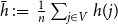
 \begin{equation} \mathcal{E}^{(r)}_i[x] \,:\!=\, \frac {1}{|N^{(r)}(i)|}\sum _{j\in N^{(r)}(i)} x(j), \qquad r\in \mathbb{N}. \end{equation}
(For
 $r=1$
we write
$r=1$
we write
 $\mathcal{E}_i[x]$
.)
$\mathcal{E}_i[x]$
.)
3.2.1 Two notions of perceived fairness
We consider two closely related perception indicators.
(i) Perception based on acceptance probabilities.
 \begin{equation} F^{(r)}_{\text{prob}}(i;\,h) \,:\!=\, \mathbf{1}\big \{\, h(i)\ \ge \ \mathcal{E}^{(r)}_i[h]\,\big \}. \end{equation}
This captures the idea that an individual evaluates whether their chance of being accepted is at least as high as the average chance observed among peers. In the running example,
 $F^{(r)}_{\mathrm{prob}}(i;\,h)$
indicates whether individual
$F^{(r)}_{\mathrm{prob}}(i;\,h)$
indicates whether individual
 $i$
perceives their acceptance probability as at least the average acceptance probability in their
$i$
perceives their acceptance probability as at least the average acceptance probability in their
 $r$
-hop neighborhood.
$r$
-hop neighborhood.
(ii) Perception based on realized outcomes.
 \begin{equation} F^{(r)}_{\text{real}}(i;\,H) \,:\!=\, \mathbf{1}\big \{\, H(i)\ \ge \ \mathcal{E}^{(r)}_i[H]\,\big \}. \end{equation}
This is the literal “I was accepted vs my neighbors” comparison, and it is random even when
 $h$
is fixed. In the running example,
$h$
is fixed. In the running example,
 $F^{(r)}_{\mathrm{real}}(i;\,H)$
captures whether the realized outcome of
$F^{(r)}_{\mathrm{real}}(i;\,H)$
captures whether the realized outcome of
 $i$
(accepted or not) compares favorably to the realized outcomes observed in their
$i$
(accepted or not) compares favorably to the realized outcomes observed in their
 $r$
-hop neighborhood.
$r$
-hop neighborhood.
Equations (4)–(5) clarify which object is being compared (probabilities vs realizations); this distinction matters for convergence statements when
 $h$
is randomized.
$h$
is randomized.
3.2.2 Fairness visibility (group-level perceived fairness)
For
 $s\in \{A,B\}$
define
$s\in \{A,B\}$
define
 \begin{equation*} \mathrm{Vis}^{\text{prob}}_r(s;\,h) \,:\!=\,\frac {1}{|V_s|}\sum _{i\in V_s} F^{(r)}_{\text{prob}}(i;\,h), \text{ and } \mathrm{Vis}^{\text{real}}_r(s;\,H) \,:\!=\,\frac {1}{|V_s|}\sum _{i\in V_s} F^{(r)}_{\text{real}}(i;\,H), \end{equation*}
 \begin{equation} \begin{cases} \Delta ^{\text{prob}}_r(h)\,:\!=\,\mathrm{Vis}^{\text{prob}}_r(A;\,h)-\mathrm{Vis}^{\text{prob}}_r(B;\,h), \\[4pt] \Delta ^{\text{real}}_r(H)\,:\!=\,\mathrm{Vis}^{\text{real}}_r(A;\,H)-\mathrm{Vis}^{\text{real}}_r(B;\,H). \end{cases} \end{equation}
We say visibility parity holds at depth
 $r$
if
$r$
if
 $\Delta _r=0$
.
$\Delta _r=0$
.
3.3 Exposure operators and degree-weighting
Besides the node-average (3), it is useful to recall the edge-weighted mean
 \begin{equation} \bar h_{\text{edge}} \,:\!=\, \frac {1}{2m}\sum _{i\in V} d_i h(i),\text{ where } m\,:\!=\,|E|. \end{equation}
This identity will be the source of classical exposure biases (friendship-paradox-type effects) in our perceived fairness gap: neighborhoods may over-sample high-degree nodes, hence over-sample high-
 $h$
nodes when
$h$
nodes when
 $h$
correlates with degree (see Proposition 5.2).
$h$
correlates with degree (see Proposition 5.2).
3.4 Asymptotics in neighborhood radius
We now formalize the idea that, on a connected graph, sufficiently large neighborhoods eventually recover population-level information.
Proposition 3.1 (Visibility convergence). Assume
 $G$
is connected and
$G$
is connected and
 $|V_s|\ge 1$
for
$|V_s|\ge 1$
for
 $s\in \{A,B\}$
. Fix a map
$s\in \{A,B\}$
. Fix a map
 $h\,:\,V\to [0,1]$
.
$h\,:\,V\to [0,1]$
.
(a) Probability-based perception.
For each
 $s\in \{A,B\}$
,
$s\in \{A,B\}$
,
 \begin{equation*} \mathrm{Vis}^{\mathrm{prob}}_r(s;\,h) \ \longrightarrow \ \mathbb{P}\big(h(i)\ge \bar h\ \big |\ S_i=s\big) \qquad \text{as } r\to \infty , \end{equation*}
where
 $\bar h\,:\!=\,\displaystyle \frac {1}{|V|}\sum _{j\in V} h(j)$
. In particular, if
$\bar h\,:\!=\,\displaystyle \frac {1}{|V|}\sum _{j\in V} h(j)$
. In particular, if
 $h$
depends only on the group (i.e.,
$h$
depends only on the group (i.e.,
 $h(i)=h_A$
on
$h(i)=h_A$
on
 $V_A$
and
$V_A$
and
 $h(i)=h_B$
on
$h(i)=h_B$
on
 $V_B$
), then
$V_B$
), then
 \begin{equation*} \mathrm{Vis}^{\mathrm{prob}}_r(s;\,h)\ \longrightarrow \ \mathbf{1}\{h_s\ge \bar h\}, \qquad \text{with } \bar h=\frac {|V_A|h_A+|V_B|h_B}{|V|}. \end{equation*}
(b) Realized-outcome perception.
Let
 $H(i)\mid h\sim \mathrm{Bernoulli}(h(i))$
independently over
$H(i)\mid h\sim \mathrm{Bernoulli}(h(i))$
independently over
 $i\in V$
. Then, conditionally on
$i\in V$
. Then, conditionally on
 $h$
, for each
$h$
, for each
 $s\in \{A,B\}$
,
$s\in \{A,B\}$
,
 \begin{equation*} \mathbb{E}\big [\mathrm{Vis}^{\mathrm{real}}_r(s;\,H)\mid h\big ] \ \longrightarrow \ \mu _s(h) + p_0(h) \qquad \text{as } r\to \infty , \end{equation*}
where
 $\mu _s(h)\,:\!=\,\displaystyle \frac {1}{|V_s|}\sum _{i\in V_s} h(i)$
and
$\mu _s(h)\,:\!=\,\displaystyle \frac {1}{|V_s|}\sum _{i\in V_s} h(i)$
and
 $p_0(h)\,:\!=\,\displaystyle \mathbb{P}(\bar H = 0 \mid h)=\prod _{j\in V}\bigl (1-h(j)\bigr )$
. In particular, if
$p_0(h)\,:\!=\,\displaystyle \mathbb{P}(\bar H = 0 \mid h)=\prod _{j\in V}\bigl (1-h(j)\bigr )$
. In particular, if
 $p_0(h)=0$
(e.g., if
$p_0(h)=0$
(e.g., if
 $\max _{j\in V} h(j)=1$
), then
$\max _{j\in V} h(j)=1$
), then
 $\mathbb{E}[\mathrm{Vis}^{\mathrm{real}}_r(s;\,H)\mid h]\to \mu _s(h)$
.
$\mathbb{E}[\mathrm{Vis}^{\mathrm{real}}_r(s;\,H)\mid h]\to \mu _s(h)$
.
Remark 3.1. The limit in (a) compares decision probabilities
 $h(i)$
to the corresponding local average and is therefore deterministic once
$h(i)$
to the corresponding local average and is therefore deterministic once
 $h$
is fixed. By contrast, (b) compares realized outcomes
$h$
is fixed. By contrast, (b) compares realized outcomes
 $H(i)$
to a realized local average, hence remains random even when
$H(i)$
to a realized local average, hence remains random even when
 $h$
is fixed; it is thus most naturally stated conditionally on
$h$
is fixed; it is thus most naturally stated conditionally on
 $h$
(and, in particular, in conditional expectation). The two notions coincide for deterministic rules (when
$h$
(and, in particular, in conditional expectation). The two notions coincide for deterministic rules (when
 $H=h$
), while for randomized rules they may differ due to global realization effects such as the event
$H=h$
), while for randomized rules they may differ due to global realization effects such as the event
 $\{\bar H=0\}$
.
$\{\bar H=0\}$
.
The proof is deferred to Section 4. On a connected finite graph, neighborhoods saturate:
 $N^{(r)}(i)=V$
for all
$N^{(r)}(i)=V$
for all
 $r\ge \mathrm{diam}(G)$
, so both visibility scores stabilize beyond the diameter. In the realized case, the conditional expectation is obtained by a direct decomposition that isolates the edge event
$r\ge \mathrm{diam}(G)$
, so both visibility scores stabilize beyond the diameter. In the realized case, the conditional expectation is obtained by a direct decomposition that isolates the edge event
 $\{\bar H=0\}$
(rather than an asymptotic law-of-large-numbers argument).
$\{\bar H=0\}$
(rather than an asymptotic law-of-large-numbers argument).
4. Analytical results and proofs
This section gathers the analytical arguments underlying the results stated in Section 3. In particular, it provides the proof of the convergence of perceived fairness as the visibility radius grows.
4.1 Convergence of perceived fairness at large visibility radius
We start by recalling a simple but fundamental topological observation.
Lemma 4.1 (Neighborhood saturation). If
 $G$
is a finite connected graph with diameter
$G$
is a finite connected graph with diameter
 $\mathrm{diam}(G)$
, then for every node
$\mathrm{diam}(G)$
, then for every node
 $i\in V$
and every
$i\in V$
and every
 $r\ge \mathrm{diam}(G)$
,
$r\ge \mathrm{diam}(G)$
,
 \begin{equation*} N^{(r)}(i)=V. \end{equation*}
Proof.
Since
 $G$
is connected, any node
$G$
is connected, any node
 $j\in V$
can be reached from
$j\in V$
can be reached from
 $i$
by a path of length at most
$i$
by a path of length at most
 $\mathrm{diam}(G)$
. Hence
$\mathrm{diam}(G)$
. Hence
 $j\in N^{(r)}(i)$
for all
$j\in N^{(r)}(i)$
for all
 $r\ge \mathrm{diam}(G)$
.
$r\ge \mathrm{diam}(G)$
.
Lemma 4.1 implies that, beyond a finite radius, all agents observe the same population-level information. This observation underlies the proof of Proposition 3.1.
4.2 Proof of Proposition 3.1
4.2.1 Probability-based perception
Recall that
 \begin{equation*} F^{(r)}_{\text{prob}}(i;\,h) =\mathbf{1}\big \{ h(i)\ge \mathcal{E}^{(r)}_i[h]\big \}. \end{equation*}
By Lemma 4.1, for all
 $r\ge \mathrm{diam}(G)$
,
$r\ge \mathrm{diam}(G)$
,
 \begin{equation*} \mathcal{E}^{(r)}_i[h] =\frac {1}{|V|}\sum _{j\in V} h(j) \,=\!:\, \bar h, \, \forall i\in V. \end{equation*}
Therefore, for all sufficiently large
 $r$
,
$r$
,
 \begin{equation*} F^{(r)}_{\text{prob}}(i;\,h) =\mathbf{1}\{\bar h\le h(i)\}. \end{equation*}
Averaging over nodes with
 $S_i=s$
yields
$S_i=s$
yields
 \begin{equation*} \mathrm{Vis}^{\text{prob}}_r(s) =\frac {1}{|V_s|}\sum _{i\in V_s}\mathbf{1}\{\bar h\le h(i)\}, \end{equation*}
which coincides with
 $\mathbb{P}\big (h(i)\ge \bar h\mid S_i=s\big )$
. This proves the convergence claim for probability-based perception.
$\mathbb{P}\big (h(i)\ge \bar h\mid S_i=s\big )$
. This proves the convergence claim for probability-based perception.
4.2.2 Realized-outcome perception
We now consider the case where realized decisions satisfy
 \begin{equation*} H(i)\mid h \sim \mathrm{Bernoulli}(h(i)),\qquad i\in V, \end{equation*}
conditionally independent given
 $h$
. By Lemma 4.1, for all
$h$
. By Lemma 4.1, for all
 $r\ge \mathrm{diam}(G)$
,
$r\ge \mathrm{diam}(G)$
,
 \begin{equation*} F^{(r)}_{\text{real}}(i;\,H) =\mathbf{1}\big \{ H(i)\ge \bar H \big \}, \qquad \bar H\,:\!=\,\frac {1}{|V|}\sum _{j\in V} H(j). \end{equation*}
Since
 $H(i)\in \{0,1\}$
and
$H(i)\in \{0,1\}$
and
 $\bar H\in [0,1]$
, we have the identity
$\bar H\in [0,1]$
, we have the identity
 \begin{equation*} \mathbf{1}\{H(i)\ge \bar H\} = H(i)+\mathbf{1}\{\bar H=0\}. \end{equation*}
Indeed, if
 $\bar H\gt 0$
then
$\bar H\gt 0$
then
 $\{H(i)\ge \bar H\}=\{H(i)=1\}$
, whereas if
$\{H(i)\ge \bar H\}=\{H(i)=1\}$
, whereas if
 $\bar H=0$
then
$\bar H=0$
then
 $\{H(i)\ge \bar H\}$
holds for all
$\{H(i)\ge \bar H\}$
holds for all
 $i$
. Therefore, for all
$i$
. Therefore, for all
 $r\ge \mathrm{diam}(G)$
,
$r\ge \mathrm{diam}(G)$
,
 \begin{equation*} F^{(r)}_{\text{real}}(i;\,H)=H(i)+\mathbf{1}\{\bar H=0\}. \end{equation*}
Taking conditional expectation given
 $h$
yields
$h$
yields
 \begin{equation*} \mathbb{E}\big[F^{(r)}_{\text{real}}(i;\,H)\mid h\big] = \mathbb{E}[H(i)\mid h]+\mathbb{P}(\bar H=0\mid h) = h(i)+p_0(h), \end{equation*}
where
 $\{\bar H=0\}=\{H(j)=0\ \forall j\in V\}$
and hence
$\{\bar H=0\}=\{H(j)=0\ \forall j\in V\}$
and hence
 \begin{equation*} p_0(h)=\mathbb{P}(H(j)=0\ \forall j\in V \mid h)=\prod _{j\in V}(1-h(j)). \end{equation*}
Averaging over
 $i\in V_s$
gives, for all
$i\in V_s$
gives, for all
 $r\ge \mathrm{diam}(G)$
,
$r\ge \mathrm{diam}(G)$
,
 \begin{equation*} \mathbb{E}\big[\mathrm{Vis}^{\text{real}}_r(s;\,H)\mid h\big] = \frac {1}{|V_s|}\sum _{i\in V_s} \bigl (h(i)+p_0(h)\bigr ) = \mu _s(h)+p_0(h), \end{equation*}
which proves the claimed convergence as
 $r\to \infty$
(the left-hand side is in fact constant for all
$r\to \infty$
(the left-hand side is in fact constant for all
 $r\ge \mathrm{diam}(G)$
).
$r\ge \mathrm{diam}(G)$
).
4.3 Extension and discussion
4.3.1 Asymptotic regimes
Proposition 3.1(b) makes explicit a subtle but important “edge case” of realized-outcome perception: when
 $\bar H=0$
(i.e., when all realized outcomes are
$\bar H=0$
(i.e., when all realized outcomes are
 $0$
), every node satisfies
$0$
), every node satisfies
 $H(i)\ge \bar H$
and hence
$H(i)\ge \bar H$
and hence
 $F^{(r)}_{\mathrm{real}}(i;\,H)=1$
for all
$F^{(r)}_{\mathrm{real}}(i;\,H)=1$
for all
 $i$
. This event contributes an additive term
$i$
. This event contributes an additive term
 $p_0(h)=\mathbb{P}(\bar H=0\mid h)=\prod _{j\in V}(1-h(j))$
to the conditional expectation of the visibility score. On a fixed finite graph, this contribution need not be negligible in general, and it is therefore natural to state the limit in terms of
$p_0(h)=\mathbb{P}(\bar H=0\mid h)=\prod _{j\in V}(1-h(j))$
to the conditional expectation of the visibility score. On a fixed finite graph, this contribution need not be negligible in general, and it is therefore natural to state the limit in terms of
 $\mu _s(h)+p_0(h)$
.
$\mu _s(h)+p_0(h)$
.
In many network settings, however, the graph size is large and the mean approval rate is bounded away from
 $0$
in the sense that
$0$
in the sense that
 $\frac {1}{|V|}\sum _{j\in V} h(j)\ge \varepsilon$
for some
$\frac {1}{|V|}\sum _{j\in V} h(j)\ge \varepsilon$
for some
 $\varepsilon \gt 0$
. In that regime, the event
$\varepsilon \gt 0$
. In that regime, the event
 $\{\bar H=0\}$
becomes exponentially unlikely since
$\{\bar H=0\}$
becomes exponentially unlikely since
 $p_0(h)=\prod _{j\in V}(1-h(j))\le \exp \!\big ({-}\sum _{j\in V} h(j)\big )\le e^{-|V|\varepsilon }$
. Consequently, the conditional expectation of realized visibility is well approximated by
$p_0(h)=\prod _{j\in V}(1-h(j))\le \exp \!\big ({-}\sum _{j\in V} h(j)\big )\le e^{-|V|\varepsilon }$
. Consequently, the conditional expectation of realized visibility is well approximated by
 $\mu _s(h)$
, which is the group-average decision probability.
$\mu _s(h)$
, which is the group-average decision probability.
The following corollary formalizes this approximation in a large-network regime.
Corollary 4.2 (Vanishing edge case). Assume we are in a regime where
 $|V|\to \infty$
and there exists
$|V|\to \infty$
and there exists
 $\varepsilon \gt 0$
such that
$\varepsilon \gt 0$
such that
 $\frac {1}{|V|}\sum _{j\in V} h(j)\ge \varepsilon$
for all graphs. Then
$\frac {1}{|V|}\sum _{j\in V} h(j)\ge \varepsilon$
for all graphs. Then
 $p_0(h)\le e^{-|V|\varepsilon }\to 0$
, and thus
$p_0(h)\le e^{-|V|\varepsilon }\to 0$
, and thus
 \begin{equation*} \mathbb{E}\big [\mathrm{Vis}^{\mathrm{real}}_r(s)\mid h\big ] \ \longrightarrow \ \mu _s(h) \quad \text{as } r\to \infty \text{ and } |V|\to \infty . \end{equation*}
4.3.2 Discussion
Corollary 4.2 shows that the discrepancy between probability-based and realized-outcome visibility is driven by a rare global event (all outcomes equal to
 $0$
). Thus, once the overall approval probability does not vanish, realized perception concentrates around the underlying probability model, and the two notions of visibility become asymptotically aligned. Conversely, when approvals are extremely sparse, the realized notion can be dominated by global randomness, which motivates treating the
$0$
). Thus, once the overall approval probability does not vanish, realized perception concentrates around the underlying probability model, and the two notions of visibility become asymptotically aligned. Conversely, when approvals are extremely sparse, the realized notion can be dominated by global randomness, which motivates treating the
 $\bar H=0$
event separately (or, in applications, adopting a small regularization of the threshold).
$\bar H=0$
event separately (or, in applications, adopting a small regularization of the threshold).
5. Topology and perceived discrimination
This section studies how network topology shapes perceived fairness at finite visibility radius. While Section 3 shows that perceived fairness converges to objective fairness as
 $r\to \infty$
, the present section focuses on the structural mechanisms that generate systematic gaps at small or moderate visibility.
$r\to \infty$
, the present section focuses on the structural mechanisms that generate systematic gaps at small or moderate visibility.
5.1 Homophily amplifies perceived discrimination
We begin with the effect of homophily. Intuitively, when individuals are more likely to connect to others from the same group, their local observations become less representative of the population, which can amplify perceived differences even under global parity.
5.1.1 Setup
We consider a
 $K$
-group stochastic block model (SBM) with group proportions
$K$
-group stochastic block model (SBM) with group proportions
 $(\pi _1,\ldots ,\pi _K)$
. Conditional on group labels, edges are independent and satisfy
$(\pi _1,\ldots ,\pi _K)$
. Conditional on group labels, edges are independent and satisfy
 \begin{equation*} \mathbb{P}[A_{ij}=1\mid S_i=S_j]=p_{\mathrm{in}}\text{ and } \mathbb{P}[A_{ij}=1\mid S_i\ne S_j]=p_{\mathrm{out}}, \end{equation*}
with
 $p_{\mathrm{in}}\gt p_{\mathrm{out}}$
(assortative mixing). We define the edge-level homophily index
$p_{\mathrm{in}}\gt p_{\mathrm{out}}$
(assortative mixing). We define the edge-level homophily index
 \begin{equation} \rho \,:\!=\,\frac {p_{\mathrm{in}}-p_{\mathrm{out}}}{p_{\mathrm{in}}+(K-1)p_{\mathrm{out}}}\in (0,1). \end{equation}
In the two-group case (
 $K=2$
), this reduces to
$K=2$
), this reduces to
 $\rho =({p_{\mathrm{in}}-p_{\mathrm{out}}})/({p_{\mathrm{in}}+p_{\mathrm{out}}})$
, and one may equivalently parameterize
$\rho =({p_{\mathrm{in}}-p_{\mathrm{out}}})/({p_{\mathrm{in}}+p_{\mathrm{out}}})$
, and one may equivalently parameterize
 $p_{\mathrm{in}}=p(1+\rho )$
and
$p_{\mathrm{in}}=p(1+\rho )$
and
 $p_{\mathrm{out}}=p(1-\rho )$
for some
$p_{\mathrm{out}}=p(1-\rho )$
for some
 $p\gt 0$
.
$p\gt 0$
.
Our homophily index (8) is a normalized within–between contrast that coincides, in the symmetric
 $K$
-SBM with
$K$
-SBM with
 $p_{\mathrm{in}}=a/n$
and
$p_{\mathrm{in}}=a/n$
and
 $p_{\mathrm{out}}=b/n$
, with the spectral ratio
$p_{\mathrm{out}}=b/n$
, with the spectral ratio
 $(a-b)/(a+(K-1)b)$
(equivalently
$(a-b)/(a+(K-1)b)$
(equivalently
 $\lambda _2/\lambda _1$
of the SBM connectivity matrix), which is standard in the community-detection literature (Abbe, Reference Abbe2017, Reference Abbe2018). Note that assortative mixing with respect to categorical labels is classically quantified via mixing matrices and assortativity coefficients (Newman, Reference Newman2002, Reference Newman2003). Here we use the normalized SBM contrast (8) as a convenient edge-level homophily index.
$\lambda _2/\lambda _1$
of the SBM connectivity matrix), which is standard in the community-detection literature (Abbe, Reference Abbe2017, Reference Abbe2018). Note that assortative mixing with respect to categorical labels is classically quantified via mixing matrices and assortativity coefficients (Newman, Reference Newman2002, Reference Newman2003). Here we use the normalized SBM contrast (8) as a convenient edge-level homophily index.
Proposition 5.1 (Homophily and perceived fairness). Assume DP holds at the population level,
 $\mathbb{E}[h(i)\mid S_i=A]=\mathbb{E}[h(i)\mid S_i=B]$
. Then, for small
$\mathbb{E}[h(i)\mid S_i=A]=\mathbb{E}[h(i)\mid S_i=B]$
. Then, for small
 $\rho$
, the group-level perceived fairness gap at depth
$\rho$
, the group-level perceived fairness gap at depth
 $r=1$
, from Equation (6), satisfies
$r=1$
, from Equation (6), satisfies
 \begin{equation*} \Delta ^{\mathrm{prob}}_1 = C\,\rho \,\Gamma (h) + o(\rho ), \end{equation*}
where
 $C\gt 0$
depends only on
$C\gt 0$
depends only on
 $(\pi _A,\pi _B)$
and
$(\pi _A,\pi _B)$
and
 $\Gamma (h)$
captures differences in local exposure across groups.
$\Gamma (h)$
captures differences in local exposure across groups.
5.1.2 Explicit form of
 $\Gamma (h)$
(neighbor-exposure contrast)
$\Gamma (h)$
(neighbor-exposure contrast)

Write
 $\mu _s \,:\!=\, \mathbb{E}[h(i)\mid S_i=s]$
for
$\mu _s \,:\!=\, \mathbb{E}[h(i)\mid S_i=s]$
for
 $s\in \{A,B\}$
and define the (depth-1) neighbor exposure
$s\in \{A,B\}$
and define the (depth-1) neighbor exposure
 \begin{equation*} h_{\mathrm{nbr}}(i) \;\,:\!=\,\; \mathcal{E}_i[h] \;=\; \frac {1}{|N(i)|}\sum _{j\in N(i)} h(j) \;=\; \frac {1}{d_i}\sum _{j\in N(i)} h(j). \end{equation*}
Let
 $\mu ^{\mathrm{nbr}}_s \,:\!=\, \mathbb{E}[h_{\mathrm{nbr}}(i)\mid S_i=s]$
. The quantity appearing in Proposition 5.1 can be written as
$\mu ^{\mathrm{nbr}}_s \,:\!=\, \mathbb{E}[h_{\mathrm{nbr}}(i)\mid S_i=s]$
. The quantity appearing in Proposition 5.1 can be written as
 \begin{equation} \Gamma (h) \;\,:\!=\, (\mu _A-\mu _B) \;-\; \big (\mu ^{\mathrm{nbr}}_A-\mu ^{\mathrm{nbr}}_B\big ). \end{equation}
In particular, under
 $\mathrm{DP}_{\mathrm{prob}}$
we have
$\mathrm{DP}_{\mathrm{prob}}$
we have
 $\mu _A=\mu _B$
, hence
$\mu _A=\mu _B$
, hence
 $\Gamma (h)=-(\mu ^{\mathrm{nbr}}_A-\mu ^{\mathrm{nbr}}_B)$
: the first-order amplification is entirely driven by differential neighborhood exposure.
$\Gamma (h)=-(\mu ^{\mathrm{nbr}}_A-\mu ^{\mathrm{nbr}}_B)$
: the first-order amplification is entirely driven by differential neighborhood exposure.
5.1.3 Remark (DP edge cases)
When DP is imposed in a way that forces
 $\mu _A=\mu _B$
exactly, the mean-shift component of the linear response cancels. A nonzero perceived gap at
$\mu _A=\mu _B$
exactly, the mean-shift component of the linear response cancels. A nonzero perceived gap at
 $r=1$
may then arise from higher-order terms and/or degree-weighted exposure effects (friendship-paradox-type sampling).
$r=1$
may then arise from higher-order terms and/or degree-weighted exposure effects (friendship-paradox-type sampling).
5.1.4 A general assortativity/modularity bound (depth
$r=1$
)

Let
 $\boldsymbol{d}\in \mathbb{R}^n$
be the degree vector,
$\boldsymbol{d}\in \mathbb{R}^n$
be the degree vector,
 $m\,:\!=\,|E|$
, and define the modularity matrix
$m\,:\!=\,|E|$
, and define the modularity matrix
 \begin{equation*} B \;\,:\!=\,\; A - \frac {\boldsymbol{d}\boldsymbol{d}^\top }{2m}. \end{equation*}
Let
 $\boldsymbol{s}\in \{\pm 1\}^n$
encode group membership (
$\boldsymbol{s}\in \{\pm 1\}^n$
encode group membership (
 $+1$
for
$+1$
for
 $\boldsymbol{A}$
,
$\boldsymbol{A}$
,
 $-1$
for
$-1$
for
 $\boldsymbol{B}$
), and define the (normalized) assortativity/modularity
$\boldsymbol{B}$
), and define the (normalized) assortativity/modularity
 \begin{equation*} Q \;\,:\!=\,\; \frac {1}{4m}\, \boldsymbol{s}^\top \boldsymbol{B} \boldsymbol{s} . \end{equation*}
Under
 $\mathrm{DP}_{\mathrm{prob}}$
and mild smoothness assumptions (implemented via a Lipschitz surrogate of the threshold map in
$\mathrm{DP}_{\mathrm{prob}}$
and mild smoothness assumptions (implemented via a Lipschitz surrogate of the threshold map in
 $F^{(1)}_{\mathrm{prob}}$
), there exists a constant
$F^{(1)}_{\mathrm{prob}}$
), there exists a constant
 $C\gt 0$
such that
$C\gt 0$
such that
 \begin{equation} \Big |\mathbb{E}\big [\Delta ^{\mathrm{prob}}_1\big ]\Big | \;\le \; C\, |Q|\, \mathrm{Lip}(h). \end{equation}
Hence, higher assortativity/modularity amplifies perceived disparity even when population-level parity holds.
5.1.5 Interpretation
Proposition 5.1 shows that homophily generates a first-order amplification of perceived unfairness, even when DP holds globally. The mechanism is purely structural: homophily changes the composition of neighborhoods, thereby distorting local comparisons without affecting population averages.
5.2 Degree bias and exposure effects
Homophily is not the only source of perceptual distortion. Even in the absence of assortative mixing, degree heterogeneity can bias local observations.
Proposition 5.2 (Degree bias at depth
 $r=1$
(edge-weighted exposure)). Assume
$r=1$
(edge-weighted exposure)). Assume
 $r=1$
and define
$r=1$
and define
 $\mathcal{E}_i[h]=\frac {1}{d_i}\sum _{j\in N(i)} h(j)$
. Then the edge-weighted average neighborhood exposure satisfies
$\mathcal{E}_i[h]=\frac {1}{d_i}\sum _{j\in N(i)} h(j)$
. Then the edge-weighted average neighborhood exposure satisfies
 \begin{equation*} \overline {\mathcal{E}}[h] \,:\!=\,\frac {1}{2m}\sum _{i\in V} d_i\,\mathcal{E}_i[h] =\frac {1}{2m}\sum _{i\in V} d_i\,h(i) =\bar h+\frac {\mathrm{Cov}(d,h)}{\mathbb{E}[d]}, \end{equation*}
where
 $\bar h\,:\!=\,\frac {1}{n}\sum _{i\in V} h(i)$
,
$\bar h\,:\!=\,\frac {1}{n}\sum _{i\in V} h(i)$
,
 $n\,:\!=\,|V|$
,
$n\,:\!=\,|V|$
,
 $2m\,:\!=\,\sum _{i\in V} d_i$
, and
$2m\,:\!=\,\sum _{i\in V} d_i$
, and
 $\mathbb{E}[d]=2m/n$
denotes the average degree (for
$\mathbb{E}[d]=2m/n$
denotes the average degree (for
 $I\sim \mathrm{Unif}(V)$
). In particular,
$I\sim \mathrm{Unif}(V)$
). In particular,
 $\overline {\mathcal{E}}[h]\gt \bar h$
iff
$\overline {\mathcal{E}}[h]\gt \bar h$
iff
 $\mathrm{Cov}(d,h)\gt 0$
.
$\mathrm{Cov}(d,h)\gt 0$
.
5.2.1 Interpretation
This is a fairness analog of the friendship paradox: when
 $h$
is positively correlated with degree, individuals are on average exposed to neighbors with higher acceptance probabilities. As a result, groups that are overrepresented among high-degree nodes may appear advantaged even under objective parity.
$h$
is positively correlated with degree, individuals are on average exposed to neighbors with higher acceptance probabilities. As a result, groups that are overrepresented among high-degree nodes may appear advantaged even under objective parity.
5.3 Clustering and variance reduction
We now turn to the role of clustering. While homophily and degree bias amplify perceived gaps, clustering has an opposite effect.
Proposition 5.3 (Clustering dampens perceived dispersion). Fix a function
 $h\,:\,V\to \mathbb{R}$
and consider depth
$h\,:\,V\to \mathbb{R}$
and consider depth
 $r=1$
neighborhood exposure
$r=1$
neighborhood exposure
 \begin{equation*} \mathcal{E}_i[h]=\frac {1}{d_i}\sum _{j\in N(i)} h(j),\qquad i\in V. \end{equation*}
Let
 $G$
and
$G$
and
 $G'$
be two graphs on the same vertex set
$G'$
be two graphs on the same vertex set
 $V$
with the same degree sequence
$V$
with the same degree sequence
 $(d_i)_{i\in V}$
, and define the exposure vectors
$(d_i)_{i\in V}$
, and define the exposure vectors
 \begin{equation*} e(G)\,:\!=\,\bigl (\mathcal{E}_i^{G}[h]\bigr )_{i\in V},\qquad e(G')\,:\!=\,\bigl (\mathcal{E}_i^{G'}[h]\bigr )_{i\in V}. \end{equation*}
Assume that there exists a doubly stochastic matrix
 $C\in \mathbb{R}^{|V|\times |V|}$
(i.e.,
$C\in \mathbb{R}^{|V|\times |V|}$
(i.e.,
 $C\mathbf{1}=\mathbf{1}$
and
$C\mathbf{1}=\mathbf{1}$
and
 $\mathbf{1}^\top C=\mathbf{1}^\top$
) such that
$\mathbf{1}^\top C=\mathbf{1}^\top$
) such that
 \begin{equation*} e(G') = C\,e(G). \end{equation*}
Then:
-
(1) The mean exposure is preserved:
$\displaystyle \frac {1}{|V|}\sum _{i\in V} e_i(G')=\frac {1}{|V|}\sum _{i\in V} e_i(G)$
. -
(2) For every convex function
$\varphi \,:\,\mathbb{R}\to \mathbb{R}$
,In particular, the dispersion of exposures cannot increase:
\begin{equation*} \frac {1}{|V|}\sum _{i\in V}\varphi \bigl (e_i(G')\bigr )\ \le \ \frac {1}{|V|}\sum _{i\in V}\varphi \bigl (e_i(G)\bigr ). \end{equation*}
\begin{equation*} \mathrm{Var}\bigl (e(G')\bigr )\ \le \ \mathrm{Var}\bigl (e(G)\bigr ). \end{equation*}


The assumption
 $e(G')=Ce(G)$
formalizes the idea that increased local clustering/overlap makes neighborhood averages more similar by turning them into convex combinations of one another.
$e(G')=Ce(G)$
formalizes the idea that increased local clustering/overlap makes neighborhood averages more similar by turning them into convex combinations of one another.
5.3.1 Interpretation
Clustering creates overlapping neighborhoods, which stabilizes local averages. As a result, individuals receive more similar signals about fairness, reducing extreme perceptions even when mean differences persist. This highlights that not all forms of segregation have the same perceptual impact: assortativity amplifies perceived gaps, whereas clustering smooths them.
5.4 Proof of Proposition 5.2
Recall that at depth
 $r=1$
,
$r=1$
,
 \begin{equation*} \mathcal{E}_i[h]=\frac {1}{d_i}\sum _{j\in N(i)} h(j), \qquad d_i\,:\!=\,|N(i)|, \qquad 2m=\sum _{i\in V} d_i. \end{equation*}
Consider the edge-weighted average neighborhood exposure (equivalently, the average over all directed neighbor observations):
 \begin{equation*} \overline {\mathcal{E}}[h] \,:\!=\,\frac {1}{2m}\sum _{i\in V} d_i\,\mathcal{E}_i[h] =\frac {1}{2m}\sum _{i\in V}\sum _{j\in N(i)} h(j). \end{equation*}
Swapping the order of summation,
 \begin{equation*} \sum _{i\in V}\sum _{j\in N(i)} h(j) =\sum _{j\in V} h(j)\,|\{i\in V:\ j\in N(i)\}| =\sum _{j\in V} h(j)\,d_j, \end{equation*}
since in an undirected graph node
 $j$
appears in exactly
$j$
appears in exactly
 $d_j$
neighborhoods. Therefore,
$d_j$
neighborhoods. Therefore,
 \begin{equation*} \overline {\mathcal{E}}[h] =\frac {1}{2m}\sum _{j\in V} d_j\,h(j). \end{equation*}
To relate this to the node-average
 $\bar h\,:\!=\,\frac 1n\sum _{j\in V} h(j)$
, note that with uniformly random
$\bar h\,:\!=\,\frac 1n\sum _{j\in V} h(j)$
, note that with uniformly random
 $I\sim \mathrm{Unif}(V)$
we have
$I\sim \mathrm{Unif}(V)$
we have
 $\mathbb{E}[d_I]=\frac {2m}{n}$
and
$\mathbb{E}[d_I]=\frac {2m}{n}$
and
 \begin{equation*} \overline {\mathcal{E}}[h] =\frac {\mathbb{E}[d_I h(I)]}{\mathbb{E}[d_I]} =\mathbb{E}[h(I)] + \frac {\mathrm{Cov}(d_I,h(I))}{\mathbb{E}[d_I]} =\bar h + \frac {\mathrm{Cov}(d,h)}{2m/n}. \end{equation*}
Hence
 $\overline {\mathcal{E}}[h]\neq \bar h$
whenever
$\overline {\mathcal{E}}[h]\neq \bar h$
whenever
 $\mathrm{Cov}(d,h)\neq 0$
, which is the claimed degree-bias (friendship-paradox-type) effect.
$\mathrm{Cov}(d,h)\neq 0$
, which is the claimed degree-bias (friendship-paradox-type) effect.
5.5 Proof of Proposition 5.3
At depth
 $r=1$
, write the vector of neighborhood averages as
$r=1$
, write the vector of neighborhood averages as
 \begin{equation*} e \,:\!=\, \bigl (\mathcal{E}_i[h]\bigr )_{i\in V} = D^{-1}A\,h, \end{equation*}
where
 $A$
is the adjacency matrix and
$A$
is the adjacency matrix and
 $D=\mathrm{diag}(d_i)$
. Let
$D=\mathrm{diag}(d_i)$
. Let
 $\mathrm{Var}(e)\,:\!=\,\frac 1n\sum _{i\in V}(e_i-\bar e)^2$
with
$\mathrm{Var}(e)\,:\!=\,\frac 1n\sum _{i\in V}(e_i-\bar e)^2$
with
 $\bar e=\frac 1n\sum _i e_i$
.
$\bar e=\frac 1n\sum _i e_i$
.
We formalize the effect of increased local clustering (with degrees held fixed) through the following sufficient condition: the new neighborhood-average vector
 $e'$
can be written as a mixing of the previous one,
$e'$
can be written as a mixing of the previous one,
 \begin{equation*} e' = C e, \end{equation*}
for some doubly stochastic matrix
 $C$
(i.e.,
$C$
(i.e.,
 $C\mathbf{1}=\mathbf{1}$
and
$C\mathbf{1}=\mathbf{1}$
and
 $\mathbf{1}^\top C=\mathbf{1}^\top$
). This captures the idea that overlapping neighborhoods (stemming from triadic closure / increased clustering) make individuals’ local averages more similar, as each
$\mathbf{1}^\top C=\mathbf{1}^\top$
). This captures the idea that overlapping neighborhoods (stemming from triadic closure / increased clustering) make individuals’ local averages more similar, as each
 $e'_i$
becomes a convex combination of nearby
$e'_i$
becomes a convex combination of nearby
 $e_j$
’s.
$e_j$
’s.
Let
 $P\,:\!=\,I-\frac 1n\mathbf{1}\mathbf{1}^\top$
be the centering projection. Since
$P\,:\!=\,I-\frac 1n\mathbf{1}\mathbf{1}^\top$
be the centering projection. Since
 $C\mathbf{1}=\mathbf{1}$
and
$C\mathbf{1}=\mathbf{1}$
and
 $\mathbf{1}^\top C=\mathbf{1}^\top$
, we have
$\mathbf{1}^\top C=\mathbf{1}^\top$
, we have
 $PC=CP$
and
$PC=CP$
and
 $Pe'=PCe=CPe$
. Moreover, any doubly stochastic matrix is a convex combination of permutation matrices (Birkhoff–von Neumann theorem), hence it is a contraction in
$Pe'=PCe=CPe$
. Moreover, any doubly stochastic matrix is a convex combination of permutation matrices (Birkhoff–von Neumann theorem), hence it is a contraction in
 $\ell _2$
on the subspace
$\ell _2$
on the subspace
 $\{\mathbf{1}\}^\perp$
:
$\{\mathbf{1}\}^\perp$
:
 \begin{equation*} \|C x\|_2 \le \|x\|_2 \quad \text{for all } x \text{ such that } \mathbf{1}^\top x=0. \end{equation*}
Applying this to
 $x=Pe$
gives
$x=Pe$
gives
 \begin{equation*} \|Pe'\|_2 = \|C(Pe)\|_2 \le \|Pe\|_2. \end{equation*}
Finally, since
 $\mathrm{Var}(e)=\frac 1n\|Pe\|_2^2$
, we obtain
$\mathrm{Var}(e)=\frac 1n\|Pe\|_2^2$
, we obtain
 \begin{equation*} \mathrm{Var}(e') \le \mathrm{Var}(e), \end{equation*}
that is, the dispersion of neighborhood averages cannot increase under such mixing. This formalizes the variance-reduction intuition: higher clustering creates overlapping neighborhoods, which stabilizes local averages and attenuates extreme perceived deviations.
5.6 Discussion
Taken together, these results show that perceived discrimination is shaped by multiple, distinct topological features. Homophily and degree heterogeneity amplify perceived unfairness by distorting local exposure, while clustering mitigates dispersion by stabilizing neighborhood-level observations. These mechanisms operate independently of population-level fairness and explain why objective parity may coexist with persistent perceived discrimination.
6. Numerical illustration and discussion
This section provides a numerical illustration of the mechanisms identified in Sections 3–5 and discusses their interpretation and implications. The simulations are intended as qualitative illustrations rather than exact tests of the theoretical results.
6.1 Numerical illustration
We simulate networks with
 $n$
nodes partitioned into two groups
$n$
nodes partitioned into two groups
 $A$
and
$A$
and
 $B$
with proportions
$B$
with proportions
 $(\pi _A,\pi _B)$
. Edges are generated according to a two-group SBM: conditional on group labels, pairs
$(\pi _A,\pi _B)$
. Edges are generated according to a two-group SBM: conditional on group labels, pairs
 $(i,j)$
are connected independently with probability
$(i,j)$
are connected independently with probability
 $p_{\mathrm{in}}$
if
$p_{\mathrm{in}}$
if
 $S_i=S_j$
and
$S_i=S_j$
and
 $p_{\mathrm{out}}$
if
$p_{\mathrm{out}}$
if
 $S_i\neq S_j$
. We parameterize homophily by
$S_i\neq S_j$
. We parameterize homophily by
 $\rho \in [0,1)$
by setting
$\rho \in [0,1)$
by setting
 $p_{\mathrm{in}}=p(1+\rho )$
and
$p_{\mathrm{in}}=p(1+\rho )$
and
 $p_{\mathrm{out}}=p(1-\rho )$
(Section 5), where
$p_{\mathrm{out}}=p(1-\rho )$
(Section 5), where
 $p\gt 0$
controls the overall density. We vary
$p\gt 0$
controls the overall density. We vary
 $\rho$
on a grid in
$\rho$
on a grid in
 $[0,\rho _{\max }]$
and generate multiple independent graph realizations for each value. Unless stated otherwise, we fix
$[0,\rho _{\max }]$
and generate multiple independent graph realizations for each value. Unless stated otherwise, we fix
 $n=400$
and
$n=400$
and
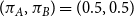 $(\pi _A,\pi _B)=(0.5,0.5)$
, and we use
$(\pi _A,\pi _B)=(0.5,0.5)$
, and we use
 $R$
independent graph realizations per value of
$R$
independent graph realizations per value of
 $\rho$
.
$\rho$
.
6.1.1 Assigning acceptance probabilities
For each simulated graph, each node
 $i$
is assigned an acceptance probability
$i$
is assigned an acceptance probability
 $h(i)\in [0,1]$
according to one of the following scenarios:
$h(i)\in [0,1]$
according to one of the following scenarios:
-
• Group-based rule:
$h(i)$
depends only on
$S_i$
(e.g.,
$h(i)=h_A$
on
$V_A$
and
$h(i)=h_B$
on
$V_B$
). -
• Degree-based rule:
$h(i)$
depends only on the node degree
$d_i$
through a monotone mapping (e.g., a normalized degree score in
$[0,1]$
). -
• Mixed rule:
$h(i)$
combines a group component and a degree component. Specifically, we set(11)where
\begin{equation} h(i)=\Pi (\alpha \,h^{\mathrm{grp}}(i) + (1-\alpha )\,h^{\mathrm{deg}}(i) + \varepsilon _i), \end{equation}
$\alpha \in (0,1)$
,
$\Pi (x)=\min \{1,\max \{0,x\}\}$
clips to
$[0,1]$
, and
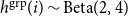
$\varepsilon _i$
is a small mean-zero noise term. In the experiments we take
$\alpha =0.7$
. We instantiate the group component by drawing
$h^{\mathrm{grp}}(i)\sim \mathrm{Beta}(4,2)$
if
$S_i=A$
and
$h^{\mathrm{grp}}(i)\sim \mathrm{Beta}(2,4)$
if
$S_i=B$
, and we set
$h^{\mathrm{deg}}(i)$
to be an increasing normalized function of
$d_i$
(e.g., rescaled ranks or
$d_i/\max _j d_j$
).


Unless stated otherwise, DP is not imposed exactly in these simulations (so the global gap may be nonzero).
6.1.2 Quantities reported
For each simulated network we compute: (i) the global (probability-based) fairness gap
 \begin{equation*} \Delta _{\mathrm{global}}(h)\,:\!=\,\frac {1}{|V_A|}\sum _{i\in V_A}h(i)-\frac {1}{|V_B|}\sum _{i\in V_B}h(i), \end{equation*}
and (ii) the perceived fairness gap at visibility radius
 $r=1$
,
$r=1$
,
 $\Delta ^{\mathrm{prob}}_1(h)=\mathrm{Vis}^{\mathrm{prob}}_1(A;\,h)-\mathrm{Vis}^{\mathrm{prob}}_1(B;\,h)$
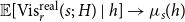
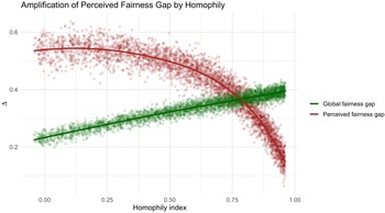
(Equation (6)). Results are displayed across realizations; in Figure 1, each point corresponds to one network realization and the solid line is a LOESS smoother.
$\Delta ^{\mathrm{prob}}_1(h)=\mathrm{Vis}^{\mathrm{prob}}_1(A;\,h)-\mathrm{Vis}^{\mathrm{prob}}_1(B;\,h)$
(Equation (6)). Results are displayed across realizations; in Figure 1, each point corresponds to one network realization and the solid line is a LOESS smoother.
6.1.3 Main observation
Figure 1 plots the perceived and global fairness gaps as functions of the homophily index
 $\rho$
. For small to moderate values of
$\rho$
. For small to moderate values of
 $\rho$
, perceived unfairness increases approximately linearly with homophily, consistent with the first-order expansion in Proposition 5.1. At larger values of
$\rho$
, perceived unfairness increases approximately linearly with homophily, consistent with the first-order expansion in Proposition 5.1. At larger values of
 $\rho$
, the perceived gap may decrease as neighborhoods become nearly homogeneous, reducing cross-group comparisons. This non-monotonic behavior does not contradict the theoretical results, which characterize local behavior around
$\rho$
, the perceived gap may decrease as neighborhoods become nearly homogeneous, reducing cross-group comparisons. This non-monotonic behavior does not contradict the theoretical results, which characterize local behavior around
 $\rho =0$
.
$\rho =0$
.
Perceived and global fairness gaps as functions of the homophily index
 $\rho$
. Each point corresponds to one network realization; solid lines show LOESS smoothing. For small to moderate homophily, perceived unfairness increases approximately linearly, while non-monotonic behavior may arise at high homophily due to neighborhood homogenization.
$\rho$
. Each point corresponds to one network realization; solid lines show LOESS smoothing. For small to moderate homophily, perceived unfairness increases approximately linearly, while non-monotonic behavior may arise at high homophily due to neighborhood homogenization.

In summary, the simulations are consistent with a positive local dependence on
 $\rho$
(as captured by Proposition 5.1), but also show that at high homophily the perceived gap may saturate or decrease.
$\rho$
(as captured by Proposition 5.1), but also show that at high homophily the perceived gap may saturate or decrease.
6.2 Interpretation and policy implications
We now discuss how the proposed framework should be interpreted and how it may inform policy analysis.
6.2.1 Perceived versus objective fairness
Perceived unfairness is not a substitute for objective fairness criteria such as DP or equality of outcomes. Rather, it captures how individuals experience fairness through local social comparisons. As shown in Sections 4 and 5, objective parity may coexist with substantial perceived unfairness when network structure distorts local exposure, and conversely low perceived unfairness may arise in highly segregated settings despite persistent demographic disparities.
6.2.2 Why perceptions matter
Perceptions of fairness influence behavior, trust, and participation in social and economic systems. Even when decisions satisfy formal fairness constraints, persistent perceived unfairness may undermine legitimacy or compliance. Our results provide a structural explanation for such mismatches by showing how network topology shapes local observations.
6.2.3 Policy objectives
Policy objectives concerning outcomes and perceptions are conceptually distinct. For realized outcomes, the goal is to reduce disparities in expected values while improving outcomes for all groups. For perceptions, the goal is to reduce systematic differences in how fairness is experienced locally. Our framework is intended to inform the latter objective by identifying how network features such as homophily, degree heterogeneity, and clustering affect perceived fairness. It does not advocate relaxing outcome-based fairness constraints.
6.2.4 Limits and extensions
Finally, we emphasize that reducing perceived unfairness through segregation or information restriction is not a desirable policy solution. While such mechanisms may mechanically reduce perceived gaps, they do so by limiting exposure rather than addressing underlying inequalities. Future work could extend the present framework to attribute-based homophily, dynamic networks, or learning processes, and study how perception and behavior co-evolve over time.
7. Discussion and extensions
This paper studies perceived fairness as a network-dependent phenomenon. While objective fairness criteria are defined at the population level, individuals evaluate fairness through local comparisons shaped by network structure. Our results show that these two perspectives may diverge systematically.
7.1 Interpretation
Perceived unfairness is not a substitute for objective fairness. Low perceived unfairness may coexist with substantial demographic disparities in segregated networks, while perceived unfairness may persist even under DP. The framework highlights this potential misalignment without advocating any normative trade-off.
7.2 Policy implications
Policy objectives concerning outcomes and perceptions are distinct. Reducing disparities in expected outcomes remains essential, but addressing persistent perceived unfairness may require complementary interventions that modify exposure or information aggregation. Network structure thus plays a critical role in how fairness is experienced.
7.3 Extensions
Several extensions are natural. Future work could study attribute-based homophily, dynamic or adaptive networks, and learning processes in which perceptions feed back into behavior. Another direction is to couple perceived fairness with endogenous network formation.
7.4 Conclusion
Perceived fairness is a structural property of networked systems. By formalizing how topology shapes local comparisons, this paper provides a unified framework to study the gap between objective and perceived fairness in social and algorithmic networks.
8. Conclusion
We proposed a mathematical framework linking network structure and perceived fairness. Our analysis highlights how local perception can deviate from global fairness even when algorithms are unbiased in aggregate. Future research will connect these theoretical insights with empirical data from collaborative or decentralized systems.
Acknowledgements
AC thanks the audience of the lecture at the at the “decentralized insurance and risk sharing” workshop at DePaul University, Chicago, in 2024. AC acknowledges the support of the Natural Sciences and Engineering Research Council of Canada (NSERC), [RGPIN-2019-07077], and the SCOR Foundation for Science.
Competing interests
None.


 Open access