


1. Introduction
Dong and Xia (Reference Dong and Xia2022), along with others, emphasize the crucial role of infrastructure investment in China’s economic growth and its function as a key tool in stabilization policy. They note that a significant portion of China’s GDP comes from infrastructure investment, which has been central to the nation’s economic expansion for decades. During downturns, infrastructure investment has consistently served as a key countercyclical measure, with the government using fiscal expansion, particularly through local government bonds, to boost investment and mitigate economic fluctuations. Between 2007 and 2016, China’s infrastructure investment saw annual double-digit growth, leading to the Chinese business cycle often being described as an “infrastructure cycle” during these years, underscoring its pivotal role in shaping the country’s economic trajectory.
Song et al. (Reference Song, Storesletten and Zilibotti2011), in an influential paper, find that the notable patterns of recent Chinese economic experience include sustained high returns on investment despite significant capital accumulation. However, they also find that state-owned enterprises (SOEs) exhibit low productivity but survive due to their preferential access to credit markets. Ansar et al. (Reference Ansar, Flyvbjerg, Budzier and Lunn2016) challenge the belief that high levels of infrastructure investment drive economic growth, arguing that such investment does not inherently create economic value and that China lacks a distinct advantage in delivering infrastructure compared to rich democracies. Dinlersoz and Fu (Reference Dinlersoz and Fu2022) find that China’s public investments have been excessive relative to the socially optimal level of investment. Rogoff and Yang (Reference Rogoff and Yang2024) find that China’s heavy reliance on real estate and infrastructure construction has led to diminishing returns, significantly contributing to local government debt vulnerabilities.
This study examines the cyclical effects of China’s deficit-financed public investments, including those in real estate and infrastructure, using a Bayesian Dynamic Stochastic General Equilibrium (DSGE) model. The model accounts for public investment inefficiency, where each dollar spent does not fully translate into an equivalent increase in public capital. Ganelli and Tervala (Reference Ganelli and Tervala2020) highlighted that the impact of public investment is significantly shaped by both its efficiency and the productivity (output elasticity) of public capital. A key finding, supported by IMF (2023) data, indicates notably low public investment efficiency in China. The Bayesian DSGE model is then used to estimate critical economic parameters, particularly the productivity of public capital, for the Chinese economy. With these estimates, the model simulates the impact of public investment on GDP and public debt in China.
We calculate that the efficiency of public investment in China is 43%, with more than half of investment expenditures failing to increase public capital. Berg et al. (Reference Berg, Buffie, Pattillo, Portillo, Presbitero and Zanna2019) attribute inefficiencies to high project costs, corruption, and poor project selection. Ansar et al. (Reference Ansar, Flyvbjerg, Budzier and Lunn2016) found that 75% of transport projects in China exceed their budgets, with costs averaging 30.6% over estimates. McMahon (Reference McMahon2018) highlights issues with unproductive state projects and empty cities, known as “white elephants.” Wedeman (Reference Wedeman2012) links public investment to rising corruption during China’s transition to a market economy, arguing that while reforms spurred growth, they also fostered corruption, undermining investment efficiency.
This study employs a Bayesian DSGE model with two key features: endogenous total factor productivity (TFP) and incomplete efficiency of public investment. TFP is highly procyclical (Fernald and Wang Reference Fernald and Wang2016; Hsu et al. Reference Hsu, Lee and Zhao2020), and the empirical literature (Brandt and Rawski Reference Brandt, Hsieh, Zhu, Brandt, Hsieh and Zhu2008; Rodrik, Reference Rodrik2014) highlights labor reallocation, scale effects, and industrial learning as the main drivers of productivity growth in China. A learning-by-doing (LBD) mechanism provides a realistic way to model endogenous TFP: higher employment generates more experience and skills, which in turn raise TFP. The model also assesses the short- and medium-term productivity effects of public investment, with efficiency set at 43% based on previous evidence.
The study’s first key finding is that the estimated output elasticity of public capital in China is only 3%, significantly lower than the 8% average found in other countries, including emerging economies, as reported by Calderón et al. (Reference Calderón, Moral-Benito and Servén2015). This indicates that the productivity of public capital in China is remarkably low. Our results directly contradict the theoretical findings of Berg et al. (Reference Berg, Buffie, Pattillo, Portillo, Presbitero and Zanna2019), who suggest that low efficiency in public investment leads to a smaller public capital stock, which in turn results in higher output elasticity. In addition, we show that the output elasticity of public capital was around 4% in 1995Q1–2008Q4 but fell to around 2% in the post-2008 period. Our findings suggest that the extensive scale of public investment in China, including real estate, may have resulted in an excess public capital stock, thereby contributing to low productivity. These findings align with Dinlersoz and Fu’s (Reference Dinlersoz and Fu2022) and Rogoff and Yang’s (Reference Rogoff and Yang2024) results, which demonstrate that excessive public investment in real estate and infrastructure has led to diminishing returns.
The DSGE model simulates the effects of fiscal policy with an efficiency parameter of 43% and an output elasticity of public capital at 3%. The second key finding is that the cumulative output multiplier of public investments over five years is 0.7, which is notably lower than empirical and theoretical estimates for advanced economies. The IMF (2015) and Gechert and Rannenberg (Reference Gechert and Rannenberg2018) report a multiplier range of 1.5–1.6 for advanced economies. Our results align with the IMF’s (2014) findings that in low-efficiency advanced countries, the five-year multiplier is 0.7. While data scarcity has limited empirical studies on public investments in emerging economies, the IMF (2014) suggests that the medium-term multiplier ranges between 0.5 and 0.9. Thus, our findings are consistent with empirical data, particularly when compared to emerging economies or those with low public investment efficiency. Our macroeconomic results support the microeconomic perspective of Ansar et al. (Reference Ansar, Flyvbjerg, Budzier and Lunn2016), who challenge the notion that China has a distinct advantage in delivering public investment compared to wealthy democracies.
A DSGE model with endogenous TFP, distortionary taxes, and private investments effectively evaluates the medium-term effects of debt-financed public investments. In the short term, these investments boost employment through increased demand, which, according to the LBD mechanism, enhances TFP. However, due to low investment efficiency and the small output elasticity of public capital, the impact on aggregate supply is minimal. Over time, the rise in public debt necessitates higher distortionary taxes, reducing employment and, consequently, TFP. Additionally, public investments crowd out more productive private investments. As a result, public investments reduce both output and TFP in the medium term, while public debt increases relative to GDP. This supports Ansar et al.’s (Reference Ansar, Flyvbjerg, Budzier and Lunn2016) assertion that while public investments may initially stimulate growth, they often fail to deliver expected benefits and instead contribute to rising debt. Our findings align with Lam and Moreno-Badia’s (Reference Lam and Moreno-Badia2023) view that China’s fiscal stimulus leads to adverse long-term effects on TFP and private investments, highlighting the complex trade-offs of such investments.
Song et al. (Reference Song, Storesletten and Zilibotti2011) discuss high returns on investment at a macro level and explore how structural imperfections, such as state interventions, shape the investment landscape in China. Our focus is narrower, analyzing specifically public investments. While Song et al. (Reference Song, Storesletten and Zilibotti2011) find that China has maintained high investment returns despite significant capital accumulation, attributing this to the reallocation from low- to high-productivity firms, even amid structural imperfections, particularly within low-productivity SOEs, our research highlights the macroeconomic challenges associated with public investments. Specifically, we find that public sector investment returns are low, and that excessive public investments are detrimental in the long term, leading to increased public debt and a decline in TFP. Our study presents a more pessimistic view of the macroeconomic effects of China’s investment-led approach.
Section 2 examines the efficiency of public investment in China, Section 3 introduces the DSGE model, and Section 4 discusses the selection and estimation of model parameters. Section 5 applies the DSGE model to analyze the effects of public investment in China, while Section 6 explores the economic policy implications.
2. Public capital stock in China
The accumulation equation for public capital, in line with Pritchett (Reference Pritchett2000) and Ganelli and Tervala (Reference Ganelli and Tervala2020), indicates that only a fraction of the total accounting cost of public investment contributes to the actual value of public capital:
 \begin{equation} K_{G,t+1}^{{}}=(1-\delta _{G})K_{G,t}^{{}}+\upsilon I_{t}^{G}, \end{equation}
where $K_{G,t}^{{}}$
represents public capital,
$K_{G,t}^{{}}$
represents public capital, $\delta _{G}$
is the depreciation rate of public capital,
$\delta _{G}$
is the depreciation rate of public capital, $I_{t}^{G}$
denotes public investment, and
$I_{t}^{G}$
denotes public investment, and $\upsilon$
(ranging between 0 and 1) reflects the efficiency of public investment. For instance, if
$\upsilon$
(ranging between 0 and 1) reflects the efficiency of public investment. For instance, if $\upsilon$
is 0.75, a one dollar increase in public investment results in a 75 cents increase in public capital. In the steady state, indicated by the subscript zero, the public capital stock is
$\upsilon$
is 0.75, a one dollar increase in public investment results in a 75 cents increase in public capital. In the steady state, indicated by the subscript zero, the public capital stock is $K_{G,0}^{{}}=\upsilon I_{0}^{G}/\delta _{G}$
. This equation also depicts the ratio of public capital stock to GDP when the proportion of GDP is utilized for public investments. IMF (2015) developed the public investment efficiency indicator, that measures the quantity and/or quality of infrastructure as output. This metric can be effectively utilized to gauge the efficiency of public investments. For advanced economies, the IMF (2015) estimated an efficiency rate of 0.87, while for emerging economies, the rate was estimated at 0.73.
$K_{G,0}^{{}}=\upsilon I_{0}^{G}/\delta _{G}$
. This equation also depicts the ratio of public capital stock to GDP when the proportion of GDP is utilized for public investments. IMF (2015) developed the public investment efficiency indicator, that measures the quantity and/or quality of infrastructure as output. This metric can be effectively utilized to gauge the efficiency of public investments. For advanced economies, the IMF (2015) estimated an efficiency rate of 0.87, while for emerging economies, the rate was estimated at 0.73.
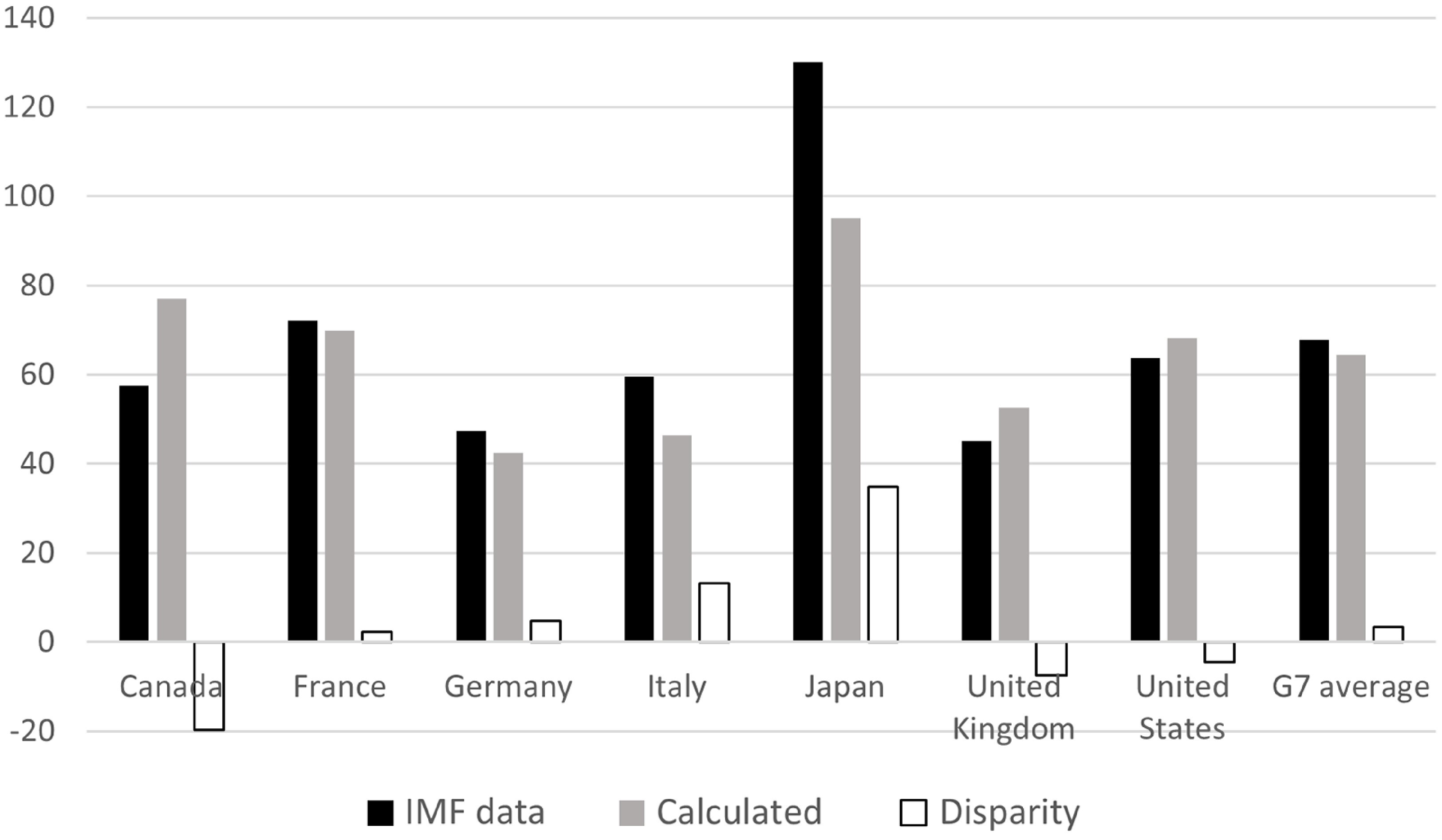
Figure 1 illustrates the level of public capital in G7 countries as a percentage of GDP, averaging data from 2010 to 2019 as provided by the IMF (2023). Additionally, it calculates the public capital stock using the public investment data for the same period (% of GDP) from the IMF (2023). This calculation applies a public investment efficiency rate of 0.87 and an estimated annual depreciation rate of public capital for advanced economies at 4.6% by the IMF (2015). According to the IMF (2023) data, the United States’ public capital amounts to 64% of its GDP. However, when calculated based on the investment rate, the figure for public capital stands at 68% of GDP ( $(0.87\times 0.035)/0.046=0.68$
). This minor discrepancy suggests that for G7 countries, Equation (1) provides an accurate depiction of the public capital stock.
$(0.87\times 0.035)/0.046=0.68$
). This minor discrepancy suggests that for G7 countries, Equation (1) provides an accurate depiction of the public capital stock.

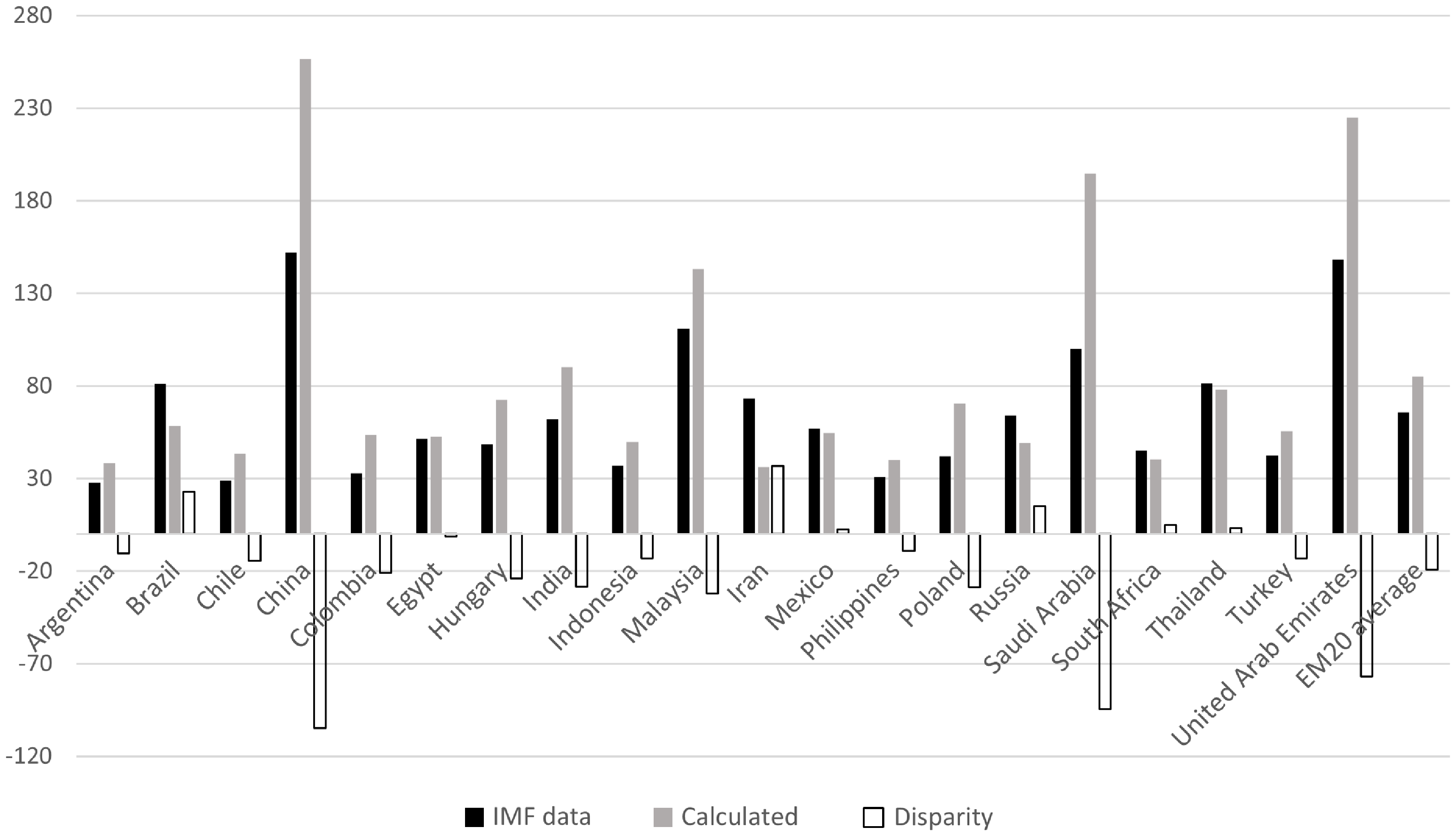
Public capital stock in EM20 countries, % of GDP.
Source: IMF (2023) and own calculations.

Figure 2 illustrates the public capital stock based on IMF (2023) data and the stock calculated from the investment rate, using IMF (2015) estimates for the efficiency of public investment in emerging economies (0.73) for the 20 most important emerging economies, defined by Duttagupta and Pazarbasioglu (Reference Duttagupta and Pazarbasioglu2021). China, Saudi Arabia, and the UAE stand out, showing significant disparities. In China, according to IMF (2023), public capital is 152% of GDP, whereas calculations based on investment rates suggest it should be 256% of GDP, leading to a disparity of 105% of GDP. Possible explanations include a very low efficiency of public investment, a higher depreciation rate of public capital relative to other countries, or measurement errors in the public capital or investment data reported by the IMF (2023). Assuming that the depreciation rate is consistent with other countries and the IMF (2023) data on public capital stock is accurate, we can calculate that the efficiency of public investment in China is 43%. Using this figure, the public capital stock in China, as derived from its investment rate (roughly 16.2%), aligns with the 152% of GDP reported by the IMF.
China’s investment inefficiency is closely tied to institutional features of its growth model. As Wedeman (Reference Wedeman2012) highlights, rapid growth has coexisted with intensifying corruption, a “double paradox” where expansion has been accompanied by systemic inefficiencies. Decentralization and interjurisdictional competition pushed local officials to prioritize large, visible projects to demonstrate growth, often causing duplication and waste. The promotion system, linking career advancement to GDP performance, further reinforced short-term investment strategies. Unlike the “developmental corruption” seen in some East Asian economies, corruption in China has been more predatory in nature, capturing rents from growth rather than supporting long-term efficiency. Local government financing vehicles added to these pressures by enabling rapid funding but reducing transparency, fostering cost overruns and misallocation. Together, these institutional drivers help explain why only 43% of public investment has translated into productive capital.
Our analysis indicates that the average efficiency of public investments is 91% in G7 countries and 64% in 20 emerging economies. If China could match these efficiency levels, it could reduce its public investment share of GDP from 16.2% to 7.7% or 11%, respectively, while still sustaining a public capital stock at 152% of GDP. Consequently, China currently wastes 8.5% or 5.2% of its GDP annually on inefficient public investments that do not contribute to the capital stock, compared to G7 or emerging countries.
3. Model
We develop a DSGE model featuring heterogeneous households, endogenous productivity, inefficiencies in public investment, and distortionary taxes. This model builds upon the framework established by Watson and Tervala (Reference Watson and Tervala2022), with modifications that incorporate inefficiency in public investment and a distinct rule for balancing the government’s finances.
3.1. Demand-side: households
Households are denoted by $z$
and are distributed uniformly along the interval between 0 and 1. Ricardian households, constituting
$z$
and are distributed uniformly along the interval between 0 and 1. Ricardian households, constituting $1-\lambda$
of the households, optimize their consumption over time. Non-Ricardian households, making up a proportion
$1-\lambda$
of the households, optimize their consumption over time. Non-Ricardian households, making up a proportion $\lambda$
, are liquidity-constrained and consume solely from their current income and endowments. All households share an identical utility function:
$\lambda$
, are liquidity-constrained and consume solely from their current income and endowments. All households share an identical utility function:
 \begin{equation*} U_{t}\left ( z\right ) =E_{t}\sum _{s=t}^{\infty }\beta ^{s-t}\epsilon _{s}^{TP} \left [ \log C_{s}-\frac {(N_{s}(z))^{1+1/\varphi }}{1+1/\varphi }\right ] , \end{equation*}
where $E$
represents the expectation operator,
$E$
represents the expectation operator, $\beta$
is the discount factor,
$\beta$
is the discount factor, $\epsilon _{t}^{TP}$
denotes time preference,
$\epsilon _{t}^{TP}$
denotes time preference, $C_{t}$
is a composite private consumption index, defined as
$C_{t}$
is a composite private consumption index, defined as $C_{t}=\left [ \int _{0}^{1}C_{t}^{{}}(z)^{\frac {\theta -1}{\theta }}dz\right ] ^{\frac {\theta }{\theta -1}}$
, where
$C_{t}=\left [ \int _{0}^{1}C_{t}^{{}}(z)^{\frac {\theta -1}{\theta }}dz\right ] ^{\frac {\theta }{\theta -1}}$
, where $C_{t}(z)$
is consumption of good
$C_{t}(z)$
is consumption of good $z$
and
$z$
and $\theta$
the elasticity of substitution between goods.
$\theta$
the elasticity of substitution between goods. $N_{t}(z)$
signifies the labor supplied in hours and
$N_{t}(z)$
signifies the labor supplied in hours and $\varphi$
denotes the Frisch elasticity of the labor supply. We posit that a time preference shock adheres to a a log-linear AR(1) process, expressed as
$\varphi$
denotes the Frisch elasticity of the labor supply. We posit that a time preference shock adheres to a a log-linear AR(1) process, expressed as $\hat {\epsilon }_{t}^{TP}=\rho ^{TP}\hat {\epsilon }_{t-1}+\hat {\varepsilon }_{t}^{TP}$
, where
$\hat {\epsilon }_{t}^{TP}=\rho ^{TP}\hat {\epsilon }_{t-1}+\hat {\varepsilon }_{t}^{TP}$
, where $\rho ^{TP}$
denotes the persistence parameter,
$\rho ^{TP}$
denotes the persistence parameter, $\hat {\varepsilon }_{t}^{TP}$
is an i.i.d. normal error term with mean zero. The hat notation indicates the percentage deviation of a variable from its steady state in a log-linearized framework. Ricardian households, which earn dividends from firms and are subject to income and consumption taxes imposed by the government, have the following resource constraint:
$\hat {\varepsilon }_{t}^{TP}$
is an i.i.d. normal error term with mean zero. The hat notation indicates the percentage deviation of a variable from its steady state in a log-linearized framework. Ricardian households, which earn dividends from firms and are subject to income and consumption taxes imposed by the government, have the following resource constraint:
 \begin{eqnarray*} \frac {R_{t}^{-1}B_{t+1}}{1-\lambda }& = &\frac {B_{t}}{1-\lambda }+\big(1-\tau _{t}^{y}\big)w_{t}N_{R,t}+\frac {\big(1-\tau _{t}^{y}\big)}{{}}\big(r_{t}^{K}K_{t}+v_{t}\big)\\[3pt]&& \big(1+\tau _{t}^{c}\big)P_{t}C_{R,t}+\frac {1}{1-\lambda }P_{t}I+\frac {\phi }{2}\Big(\frac {I_{t}}{K_{t}}-\delta \Big)^{2}, \end{eqnarray*}
where $N_{R,t}$
and
$N_{R,t}$
and $C_{R,t}$
represent the labor supply and consumption of Ricardian households, the model includes
$C_{R,t}$
represent the labor supply and consumption of Ricardian households, the model includes $B_{t}$
the nominal price of a government bond with a payoff of $1 maturing at
$B_{t}$
the nominal price of a government bond with a payoff of $1 maturing at $t+1$
and
$t+1$
and $r_{t}$
its nominal yield. The nominal wage is denoted as
$r_{t}$
its nominal yield. The nominal wage is denoted as $w_{t}$
,
$w_{t}$
, $v_{t}$
reflects the financial returns from fully dividend-imputed firms, taxed similarly to household income. Tax rates on income and consumption are represented by
$v_{t}$
reflects the financial returns from fully dividend-imputed firms, taxed similarly to household income. Tax rates on income and consumption are represented by $\tau ^{y}$
and
$\tau ^{y}$
and $\tau ^{c}$
, respectively. The return on private capital is
$\tau ^{c}$
, respectively. The return on private capital is $r_t^k$
, and
$r_t^k$
, and $P_t$
is the price index, defined as
$P_t$
is the price index, defined as $P_t = \left [ \int _{0}^{1} P_t(z)^{1-\theta }\, dz \right ]^{\frac {1}{1-\theta }}$
, where
$P_t = \left [ \int _{0}^{1} P_t(z)^{1-\theta }\, dz \right ]^{\frac {1}{1-\theta }}$
, where $P_t(z)$
is the price of good
$P_t(z)$
is the price of good $z$
. Private investment is
$z$
. Private investment is $I_{t}$
with quadratic adjustment costs expressed as
$I_{t}$
with quadratic adjustment costs expressed as $\phi (\cdot )=$ $\phi /2(I_{t}/K_{t}-\delta )^{2}$
, and
$\phi /2(I_{t}/K_{t}-\delta )^{2}$
, and $\delta$
is the depreciation rate of private capital. The accumulation of private capital is
$\delta$
is the depreciation rate of private capital. The accumulation of private capital is $K_{t+1}=(1-\delta )K_{t}+I_{t}$
.
$K_{t+1}=(1-\delta )K_{t}+I_{t}$
.
The conditions for optimal behavior of Ricardian households are as follows:
 \begin{equation} \beta R_{t}E_{t}\bigg (\frac {\epsilon _{t+1}^{TP}(1+\tau _{t}^{c})P_{t}C_{R,t}}{\epsilon _{t}^{TP}(1+\tau _{t+1}^{c})P_{t+1}C_{R,t+1}}\bigg )=1, \end{equation}
 \begin{equation} N_{R,t}(z)=\bigg (\frac {(1-\tau _{t}^{y})w_{t}}{C_{R,t}(1+\tau _{t}^{c})P_{t}}\bigg )^{\varphi }. \end{equation}
 \begin{equation} q_{t}=1+\phi \bigg (\frac {I_{t}}{K_{t}}-\delta \bigg ), \end{equation}
 \begin{equation} q_{t}=E_{t}\bigg \{\Lambda _{t,t+1}\bigg [\big(1-\tau _{t+1}^{y}\big)r_{t+1}^{K}+q_{t+1}(1-\delta )-\phi _{t+1}+\bigg (\frac {I_{t+1}}{K_{t+1}}\bigg )\phi _{t+1}^{^{\prime }}\bigg ]\bigg \}, \end{equation}
where $\Lambda _{t,t+1}=\beta \bigg (\frac {C_{R,t}}{C_{R,t+1}}\bigg )$
. Furthermore, we assume that the log-linearized version of the investment equation incorporates investment shocks (IS), which follow a similar AR(1) process as the other shocks in the model.
$\Lambda _{t,t+1}=\beta \bigg (\frac {C_{R,t}}{C_{R,t+1}}\bigg )$
. Furthermore, we assume that the log-linearized version of the investment equation incorporates investment shocks (IS), which follow a similar AR(1) process as the other shocks in the model.
Non-Ricardian households, receiving income from working in firms and public transfers while paying taxes, have these optimal conditions:
 \begin{equation} \big(1+\tau _{t}^{c}\big)P_{t}C_{N,t}=\big(1-\tau _{t}^{y}\big)w_{t}N_{N,t}+\omega \frac {G_{t}^{T}}{\lambda }, \end{equation}
 \begin{equation} N_{N,t}(z)=\bigg (\frac {(1-\tau _{t}^{y})w_{t}}{C_{N,t}(1+\tau _{t}^{c})P_{t}}\bigg )^{\varphi }, \end{equation}
Aggregate consumption and labor supply are then defined as $C_{t}=\lambda C_{N,t}+(1-\lambda )C_{R,t}$
and
$C_{t}=\lambda C_{N,t}+(1-\lambda )C_{R,t}$
and $N_{t}=\lambda N_{N,t}+(1-\lambda )N_{R,t}$
.
$N_{t}=\lambda N_{N,t}+(1-\lambda )N_{R,t}$
.
3.2. Supply-side: firms
China’s rapid growth from the 1990s to the 2010s was driven largely by industrialization and a massive reallocation of labor from agriculture to manufacturing, rather than by high-tech innovation. Empirical studies (Brandt et al. Reference Brandt, Hsieh, Zhu, Brandt, Hsieh and Zhu2008; Rodrik, Reference Rodrik2014) highlight labor reallocation, scale effects, and industrial learning as key drivers of productivity growth. A LBD mechanism therefore provides a natural way to model endogenous TFP: higher employment generates more experience and skills, which in turn raise TFP. By contrast, knowledge-capital models are more suitable for economies where R&D spending is the primary engine of growth, while variety-expansion models better capture innovation-driven growth in high-tech, open economies. Moreover, TFP strongly correlates with GDP, as shown in studies such as Fernald and Wang (Reference Fernald and Wang2016) and Hsu et al. (Reference Hsu, Lee and Zhao2020). To introduce endogenous and procyclical TFP in a DSGE model, a LBD equation can be used, as exemplified by Chang et al. (Reference Chang, Gomes and Schorfheide2002), Engler and Tervala (Reference Engler and Tervala2018), and Watson and Tervala (Reference Watson and Tervala2022):
 \begin{equation} Y_{t}(z)=K_{t}(z)^{\alpha }(N_{t}(z)X_{t})^{1-\alpha }K_{G,t}^{\phi _{kg}}. \end{equation} $Y_{t}(z)$
denotes the output of firm
$Y_{t}(z)$
denotes the output of firm $z$
,
$z$
, $K_{G,t}$
represents public capital,
$K_{G,t}$
represents public capital, $\phi _{kg}$
indicating the output elasticity of this public capital.
$\phi _{kg}$
indicating the output elasticity of this public capital. $X_{t}$
is defined as TFP, encapsulating the overall productivity level that includes the skill level of the average worker and other efficiency factors.
$X_{t}$
is defined as TFP, encapsulating the overall productivity level that includes the skill level of the average worker and other efficiency factors. $X_{t}$
is modeled to depend on past working hours, reflecting a LBD process, with its dynamics governed by the following law of motion:
$X_{t}$
is modeled to depend on past working hours, reflecting a LBD process, with its dynamics governed by the following law of motion:
 \begin{equation} X_{t}=X_{t-1}^{\rho _{x}}N_{t-1}^{\mu _{l}}(z), \end{equation}
where $\rho _{x}$
denotes the persistence of accumulated TFP stock, while
$\rho _{x}$
denotes the persistence of accumulated TFP stock, while $\mu _{l}$
denotes the elasticity of TFP relative to the hours of employment in the preceding period.
$\mu _{l}$
denotes the elasticity of TFP relative to the hours of employment in the preceding period.
Cost minimization leads to a ratio of capital to labor
 \begin{equation} \frac {K_{t}(z)}{N_{t}(z)}=\frac {\alpha }{1-\alpha }\frac {w_{t}}{r_{t}^{K}}. \end{equation}
Firms aim to maximize the present value of their profits, denoted as $v_{t}(z)$
 \begin{equation} \max _{p_{t}(z)}{v_{t}(z)}=E_{t}\sum _{s=t}^{\infty }\gamma ^{s-t}Q_{t,s}\frac {v_{s}(z)}{P_{s}}, \end{equation}
where $1-\gamma$
represents the likelihood of a firm being able to adjust its price in any given period. Given the stochastic discount factor
$1-\gamma$
represents the likelihood of a firm being able to adjust its price in any given period. Given the stochastic discount factor $\xi _{t,s}$
between periods
$\xi _{t,s}$
between periods $t$
and
$t$
and $s$
, the solution for
$s$
, the solution for $p_{t}(z)$
can be expressed as
$p_{t}(z)$
can be expressed as
 \begin{equation} p_{t}(z)=\frac {\theta }{\theta -1}\frac {E_{t}\sum _{s=t}^{\infty }\gamma ^{s-t}\xi _{t,s}Q_{s}MC_{s}(z)}{E_{t}\sum _{s=t}^{\infty }\gamma ^{s-t}\xi _{t,s}Q_{s}}, \end{equation}
where
 \begin{equation*} Q=\left ( \frac {C_{s}+I_{s}+\phi \big(\frac {I_{s}}{K_{s}}\big)K_{s}+G_{s}^{C}+I_{s}^{G}}{P_{s}}\right )\!. \end{equation*}
Log-linearizing equation (12) yields the pricing equation $\hat {p}_{t}(z)=\beta \gamma E_{t}(\hat {p}_{t+1}(z))$ $+(1-\beta \gamma )(\hat {mc}_{t}(z))+\epsilon _{t}^{CP}$
, where
$+(1-\beta \gamma )(\hat {mc}_{t}(z))+\epsilon _{t}^{CP}$
, where $\epsilon _{t}^{CP}$
represents a cost-push shock. It follows a similar AR(1) process as the other shocks within the framework. The overall price level is determined by
$\epsilon _{t}^{CP}$
represents a cost-push shock. It follows a similar AR(1) process as the other shocks within the framework. The overall price level is determined by $\hat {p}_{t}=\gamma \hat {p}_{t-1}+(1-\gamma )\hat {p}_{t}(z)$
.
$\hat {p}_{t}=\gamma \hat {p}_{t-1}+(1-\gamma )\hat {p}_{t}(z)$
.
3.3. Economic policy
The equation depicting the accumulation of public capital, Equation (1), is presented and elaborated upon in the introductory section. It is assumed that public consumption indices mirror those of private consumption, with public demand functions for domestic goods formulated similarly to private demand functions. The budget constraint for the government is as follows:
 \begin{equation} \tau _{t}^{y}\big(w_{t}N_{t}+r_{t}^{K}K_{t}+v_{t}\big)+\tau _{t}^{c}P_{t}C_{t}=B_{t}-R_{t}^{-1}B_{t+1}+P_{t}\big(G_{t}^{C}+I_{t}^{G}+G_{t}^{T}\big). \end{equation}
The Government responds to variations in the previous period’s public debt relative to its initial steady state level by adjusting the income tax burden:
 \begin{equation} \tau _{t}^{y}=\tau _{0}^{y}\bigg (B_{t-1}-B_{0}\bigg )^{\Phi _{d}}. \end{equation}
The tax elasticity in relation to public debt is denoted by is $\Phi _{d}.$
Each category of government expenditure, denoted as
$\Phi _{d}.$
Each category of government expenditure, denoted as $\hat {g}$
(where
$\hat {g}$
(where $g$
represents
$g$
represents $G^{C}$
,
$G^{C}$
, $I^{G}$
, and
$I^{G}$
, and $G^{T}$
) follows an AR(1) process:
$G^{T}$
) follows an AR(1) process: $\hat {g}_{g,t}=\rho ^{g}\hat {g}_{g,t-1}+\varepsilon _{g,t}^{g}$
. Here
$\hat {g}_{g,t}=\rho ^{g}\hat {g}_{g,t-1}+\varepsilon _{g,t}^{g}$
. Here $\rho ^{g}$
ranges from zero to one,
$\rho ^{g}$
ranges from zero to one, $\hat {g}_{g,t}$
is defined as
$\hat {g}_{g,t}$
is defined as $(G_{g,t}-G_{g,0})/Y_{0}$
,
$(G_{g,t}-G_{g,0})/Y_{0}$
, $\epsilon _{g,t}^{g}$
is an independent and identically distributed spending shock variable with a mean of zero.
$\epsilon _{g,t}^{g}$
is an independent and identically distributed spending shock variable with a mean of zero.
Monetary policy conforms to a Taylor (Reference Taylor1993) rule, incorporating interest rate smoothing. The log-linearized version of this monetary policy rule is as follows:
 \begin{equation*} \hat {\imath }_{t}=\mu _{s}\hat {\imath }_{t-1}+(1-\mu _{s})(\mu _{p}\Delta \hat {P}_{t}+\mu _{y}\hat {Y}_{t})+\hat {\varepsilon }_{t}^{r}, \end{equation*}
where $\Delta$
is the first difference operator and
$\Delta$
is the first difference operator and $\hat {\varepsilon }_{t}^{r}$
indicates a monetary policy shock characterized by a zero mean.
$\hat {\varepsilon }_{t}^{r}$
indicates a monetary policy shock characterized by a zero mean.
4. Parameter values
4.1. Parameterization
Consistent with conventional parameters in DSGE literature, the discount factor ( $\beta$
) is established at 0.995, and the elasticity of substitution between goods (
$\beta$
) is established at 0.995, and the elasticity of substitution between goods ( $\theta$
) is determined to be 6. The Frisch elasticity of labor supply (
$\theta$
) is determined to be 6. The Frisch elasticity of labor supply ( $\varphi$
) is established at 2, reflecting the perspective that the macro Frisch elasticity is high (Peterman, Reference Peterman2016). The proportion of Non-Ricardian households (
$\varphi$
) is established at 2, reflecting the perspective that the macro Frisch elasticity is high (Peterman, Reference Peterman2016). The proportion of Non-Ricardian households ( $\lambda$
) is 35%, based on the estimates for the Chinese economy by Liu and Ou (Reference Liu and Ou2020). The consumption tax rate (
$\lambda$
) is 35%, based on the estimates for the Chinese economy by Liu and Ou (Reference Liu and Ou2020). The consumption tax rate ( $\tau ^{c}$
) is established at 0.1, aligned with China’s standard value-added tax rates (6%, 9%, or 12%) and the effective consumption tax rate estimated by Miao et al. (Reference Miao and Bai2023). The tax rate (
$\tau ^{c}$
) is established at 0.1, aligned with China’s standard value-added tax rates (6%, 9%, or 12%) and the effective consumption tax rate estimated by Miao et al. (Reference Miao and Bai2023). The tax rate ( $\tau _{t}^{y}$
) is set at 0.4, exceeding the OECD’s (2021) estimate of the tax wedge. China’s public finances have seen chronic deficits, with a fiscal surplus occurring in only one year between 1995 and 2007. The model’s considerable public expenditures and the requirement for fiscal balance to ensure stability necessitate a tax rate higher than the OECD’s estimate.
$\tau _{t}^{y}$
) is set at 0.4, exceeding the OECD’s (2021) estimate of the tax wedge. China’s public finances have seen chronic deficits, with a fiscal surplus occurring in only one year between 1995 and 2007. The model’s considerable public expenditures and the requirement for fiscal balance to ensure stability necessitate a tax rate higher than the OECD’s estimate.
In macroeconomic models focused on China, the output elasticity of private capital ( $\alpha$
) is typically higher than in advanced economies, reflecting China’s more capital-intensive production and a labor share of GDP that has been just over 50% (United Nations, 2023). Li and Liu (Reference Li and Liu2017) use a figure of 0.4, while Fernandez-Villaverde et al. (Reference Fernandez-Villaverde, Ohanian and Yao2023) opt for 0.5. We set the share of private capital at 0.45, in line with Lei et al. (Reference Lei, Yao and Peng2023). The efficiency of public investment (
$\alpha$
) is typically higher than in advanced economies, reflecting China’s more capital-intensive production and a labor share of GDP that has been just over 50% (United Nations, 2023). Li and Liu (Reference Li and Liu2017) use a figure of 0.4, while Fernandez-Villaverde et al. (Reference Fernandez-Villaverde, Ohanian and Yao2023) opt for 0.5. We set the share of private capital at 0.45, in line with Lei et al. (Reference Lei, Yao and Peng2023). The efficiency of public investment ( $\upsilon$
) in China is set at 43%.
$\upsilon$
) in China is set at 43%.
The analysis employs data from “China’s Macroeconomy: Time Series Data” by Chang et al. (Reference Chang, Chen, Waggoner and Zha2015, Reference Chang, Chen, Waggoner and Zha2023), covering all relevant variables from 1995:Q1 to 2017:Q4. The ratio of public debt-to-annual GDP has averaged 32% over the entire period (Mbaye et al. Reference Mbaye, Moreno-Badia and Chae2018). In our model, the debt ratio is set to 128% relative to quarterly GDP. Public investments, including state-owned and holding enterprises, averaged 22% over the entire period, but reduced to 18% in the last decade after excluding net exports’ contribution to GDP. Public consumption expenditures remained steady at 16% throughout the entire period and the last ten years. We set the share of public investments at 18% and public consumption at 16%. In our model, the GDP shares of private consumption and investment are determined endogenously through the model’s parameters and are 47 and 19%, respectively. According to the data (Chang et al. Reference Chang, Chen, Waggoner and Zha2015, Reference Chang, Chen, Waggoner and Zha2023), the GDP share of private consumption (investment) has been 38% (27%) over the past decade and 43% (19%) over the entire period.
4.2. Prior distribution of the parameters
The remaining model parameters are estimated utilizing Bayesian techniques. The dataset for estimation encompasses quarterly real GDP, private consumption, private investment, public investment, and price level, sourced from Chang et al. (Reference Chang, Chen, Waggoner and Zha2015, Reference Chang, Chen, Waggoner and Zha2023). Their dataset aligns with U.S. national accounts definitions while retaining the specific features of Chinese data, making it well-suited for our Bayesian estimation. Additionally, the quarterly average interest rate is derived from monthly data (discount rate for China) obtained from the Fred Economic Data (2023).
Public investment is measured as the sum of gross fixed capital formation by the government and by SOEs, ensuring that the measure captures both direct government investment and investment undertaken through SOEs. Private investment is defined as total gross fixed capital formation excluding inventories, net of public investment. All data are represented in log-deviations from their Hodrick-Prescott (Reference Hodrick and Prescott1997) trends (using a smoothing parameter of 1600). The estimation process employs data spanning from 1995Q1 to 2017Q4, since investment series such as gross fixed capital formation by the government and SOEs are available at a quarterly frequency only for this period. The stochastic dynamics of the model are determined by seven exogenous disturbances: three kinds of public spending shocks (consumption, investment, and transfers), a monetary policy shock, a private IS, a time preference shock, and a cost-push shock.
Watson and Tervala (Reference Watson and Tervala2021) estimated a LBD equation using Australian data. They found the persistence of TFP to be 0.91, and the elasticity of TFP relative to employment averaged 0.25. The prior for the persistence of TFP ( $\rho _{x}$
) is set at 0.91 with a standard deviation of 0.05. The persistence of all AR(1) processes follows a beta distribution. The prior for the elasticity of TFP relative to employment (
$\rho _{x}$
) is set at 0.91 with a standard deviation of 0.05. The persistence of all AR(1) processes follows a beta distribution. The prior for the elasticity of TFP relative to employment ( $\mu _{l}$
) is assumed to be 0.25, characterized by a Normal distribution with a standard deviation of 0.1.
$\mu _{l}$
) is assumed to be 0.25, characterized by a Normal distribution with a standard deviation of 0.1.
The prior for the elasticity of taxes in relation to public debt ( $\Phi _{d}$
) is set at 0.075, reflecting the average of the values used by Lieberknecht and Wieland (Reference Lieberknecht and Wieland2019). Its standard deviation is 0.1. Furthermore, the parameter is assigned a lower bound of 0.0001 to guarantee long-term stability in the public debt level. Numerous studies have estimated the output elasticity of public capital (
$\Phi _{d}$
) is set at 0.075, reflecting the average of the values used by Lieberknecht and Wieland (Reference Lieberknecht and Wieland2019). Its standard deviation is 0.1. Furthermore, the parameter is assigned a lower bound of 0.0001 to guarantee long-term stability in the public debt level. Numerous studies have estimated the output elasticity of public capital ( $\phi _{kg}$
) in advanced economies, as outlined in a survey by Bom and Ligthart (Reference Bom and Ligthart2013). Calderón et al. (Reference Calderón, Moral-Benito and Servén2015) estimated the output elasticity of public capital across a sample of 88 countries spanning various income levels. Their findings (referenced in Tables 3 and 4) indicate an average productivity of public capital at 0.08, showing no significant variation in relation to a country’s per capita income, infrastructure endowment, or population size. Based on this, we have selected 8% as our parameter value, with an accompanying standard deviation of 0.1. Additionally, a lower bound of 0.0001 is assigned to the parameter.
$\phi _{kg}$
) in advanced economies, as outlined in a survey by Bom and Ligthart (Reference Bom and Ligthart2013). Calderón et al. (Reference Calderón, Moral-Benito and Servén2015) estimated the output elasticity of public capital across a sample of 88 countries spanning various income levels. Their findings (referenced in Tables 3 and 4) indicate an average productivity of public capital at 0.08, showing no significant variation in relation to a country’s per capita income, infrastructure endowment, or population size. Based on this, we have selected 8% as our parameter value, with an accompanying standard deviation of 0.1. Additionally, a lower bound of 0.0001 is assigned to the parameter.
The priors for the quarterly depreciation rates of private ( $\delta$
) and public capital are set at 0.025 and 0.0125, respectively, to align the annual depreciation rates with the estimates of 10% and roughly 5% as determined by the IMF (2015). The standard deviation for these rates is set at a low value of 0.05, reflecting the minimal uncertainty associated with these parameters.
$\delta$
) and public capital are set at 0.025 and 0.0125, respectively, to align the annual depreciation rates with the estimates of 10% and roughly 5% as determined by the IMF (2015). The standard deviation for these rates is set at a low value of 0.05, reflecting the minimal uncertainty associated with these parameters.
Smets and Wouters (Reference Smets and Wouters2007) initially set the priors for the persistence of all types of public spending shocks at 0.5. However, numerous studies have identified significantly higher values, reaching up to 0.94, as found by Sims and Wolff (Reference Sims and Wolff2018). As a compromise, we adopt a value of 0.75, similar to what Iwata (Reference Iwata2013) discovered for public consumption and investment. The standard deviation for these rates is set at 0.1. The priors for the persistence of other shocks, time preference, cost-push, and investment, are set at 0.5, following Smets and Wouters (Reference Smets and Wouters2007), with standard deviations assigned a value of 0.2. We select a gamma distribution for the standard deviation of all shocks, setting the mean at 0.5 and the standard deviation at 0.4.
The Calvo parameter ( $\gamma$
) is set at 0.75, a standard value in DSGE macro modeling, with its standard deviation fixed at 0.05. The priors for parameters characterizing monetary policy are in line with Smets and Wouters (Reference Smets and Wouters2007). The responses to inflation (
$\gamma$
) is set at 0.75, a standard value in DSGE macro modeling, with its standard deviation fixed at 0.05. The priors for parameters characterizing monetary policy are in line with Smets and Wouters (Reference Smets and Wouters2007). The responses to inflation ( $\mu _{p}$
) and output (
$\mu _{p}$
) and output ( $\mu _{y}$
) are described by a Normal distribution with means of 1.5 and 0.125 (a quarter of 0.5), and standard errors of 0.1 and 0.05, respectively. The smoothing parameter (
$\mu _{y}$
) are described by a Normal distribution with means of 1.5 and 0.125 (a quarter of 0.5), and standard errors of 0.1 and 0.05, respectively. The smoothing parameter ( $\mu _{s}$
) is set at 0.75, with a standard deviation of 0.05, following a Beta distribution. The prior for the investment adjustment cost parameter (
$\mu _{s}$
) is set at 0.75, with a standard deviation of 0.05, following a Beta distribution. The prior for the investment adjustment cost parameter ( $\phi$
) is set at 4, as per Smets and Wouters (Reference Smets and Wouters2007), with a standard deviation of 1.
$\phi$
) is set at 4, as per Smets and Wouters (Reference Smets and Wouters2007), with a standard deviation of 1.
4.3. Posterior Estimates of the Parameters
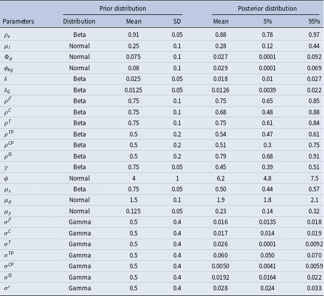
Table 1 presents the posterior means and credible intervals of the model parameters, determined using Bayesian Highest Density Intervals (HDI). Figure 3 illustrates the prior (in gray) and posterior (in black) distributions of key variables. The Metropolis-Hastings (MH) algorithm chain’s initial value is set at 0.3, and the scale parameter for the covariance matrix in the Random Walk MH algorithm is 0.4. This configuration results in an acceptance rate of 24%, aligning well with the optimal acceptance ratio of 23% as suggested by Roberts et al. (Reference Roberts, Gelman and Gilks1997). For the MH algorithm, five parallel chains are utilized. In accordance with Smets and Wouters (Reference Smets and Wouters2007), the MH algorithm runs through 250,000 Markov chain Monte Carlo replications. Additionally, we set the fraction of initially generated parameter vectors to be excluded at 0.5, thereby discarding the first 125,000 draws.
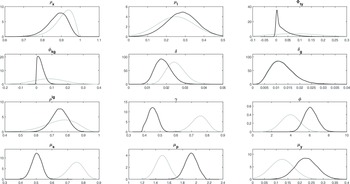
Prior and posterior distributions of model parameters

Prior (gray) and posterior (black) distributions of main variables.

The model lends support to the LBD equation: greater employment raises TFP. The posterior persistence of TFP is somewhat lower than both the prior estimate and the findings of Watson and Tervala (Reference Watson and Tervala2022) for Australia. By contrast, the elasticity of TFP with respect to employment is higher than both the prior and their results, indicating a significant role of employment in driving TFP. As Rodrik (Reference Rodrik2014) notes, rapid growth in developing economies is often driven by labor reallocation into modern, productivity-enhancing industries where workers accumulate know-how through production. Our model captures this process by linking TFP to employment, reflecting how structural transformation and industrialization boost productivity through experience-based gains.
For many variables, the mean of the posterior distribution is relatively close to the mean of the prior. However, the tax elasticity with respect to public debt is relatively small in China. In addition, the posterior estimate for the productivity of public capital is significantly lower, at 2.9%, compared to the prior of 8%. Additionally, the confidence interval for this estimate is quite narrow. The productivity of public capital may not be constant but has likely declined over time as the capital stock has accumulated. The likely cause of the low efficiency of public investment is the extensive scale of public investment, including real estate, which has resulted in an excess public capital stock, including housing. Lam and Moreno-Badia (Reference Lam and Moreno-Badia2023) find weak performance and returns of SOEs and declining infrastructure returns in China.
It is plausible that the productivity of public capital has declined over time as China has undertaken massive infrastructure development. The full-sample estimate of 3% likely reflects an average that masks a higher elasticity in the early years and a lower one more recently. To test this hypothesis, we re-estimated the model separately for 1995Q1–2008Q4 and 2009Q1–2017Q4. The results show that the output elasticity of public capital was nearly 4% (0.036) in the earlier period but fell to around 2% in the later period. These findings offer quantitative support for the view that the marginal productivity of public capital has declined as the scale of investment has expanded, consistent with the narrative of diminishing returns to China’s public investment boom.
While our model treats public investment as a single aggregate, in reality it consists of heterogeneous components, including infrastructure (transport, energy) and real estate, each with potentially different levels of productivity. As documented by Rogoff and Yang (Reference Rogoff and Yang2024), China’s investment boom has been heavily concentrated in real estate and infrastructure. Much of the new construction has taken place in lower-tier cities, where population growth and economic activity have been weak. This pattern may partly explain why we find a declining output elasticity of public capital over time: the earlier phase of investment likely delivered higher-return infrastructure, while the later phase has increasingly produced real estate projects with limited economic payoff, consistent with diminishing returns at the aggregate level.
The posterior estimate of the depreciation rate of public capital (1.26%) closely aligns with its prior estimate of 1.25%. This corresponds to an annual depreciation rate of 4.9% $(1-(1-0.0126) \,^{\hat {}}\, 4=0.049)$
, which is only slightly higher than the 4.6% annual rate used in the calculations in Section 2. As discussed in Section 2, possible explanations for the large disparity between the stock of public capital and the level implied by the investment rate include a very low efficiency of public investment, a higher depreciation rate of public capital, or measurement errors in the public capital or investment data. Hence, the bulk of the discrepancy is likely explained by the low efficiency of public investment. Using the estimated annual depreciation rate of 4.9%, we calculate that the efficiency of public investment in China is 46%, which represents only a very small change compared with the 43% reported in Section 2.
$(1-(1-0.0126) \,^{\hat {}}\, 4=0.049)$
, which is only slightly higher than the 4.6% annual rate used in the calculations in Section 2. As discussed in Section 2, possible explanations for the large disparity between the stock of public capital and the level implied by the investment rate include a very low efficiency of public investment, a higher depreciation rate of public capital, or measurement errors in the public capital or investment data. Hence, the bulk of the discrepancy is likely explained by the low efficiency of public investment. Using the estimated annual depreciation rate of 4.9%, we calculate that the efficiency of public investment in China is 46%, which represents only a very small change compared with the 43% reported in Section 2.
The annual depreciation rate of private capital is about 7%, which is fairly close to the IMF’s (2015) estimate for middle-income countries. The estimated persistence of public ISs is 0.75. The posterior estimate for the Calvo parameter is 0.45, indicating that the average age of prices is approximately two quarters. This value is quite typical and aligns closely with the result of 0.39 obtained by Liu and Ou (Reference Liu and Ou2020) for China. The posterior estimate for the investment adjustment cost parameter is 6.2, which is relatively close to the estimate of 5.7 provided by Smets and Wouters (Reference Smets and Wouters2007). The posterior estimates for the coefficients of the monetary policy rule imply relatively modest smoothing and a fairly strong response to inflation and output fluctuations.
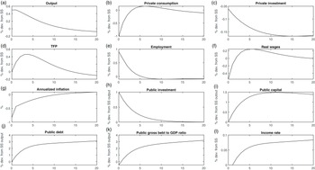
5. Fiscal multiplier of public investment
In this section, we examine the effects of public investments when the model’s parameters are set to match the calibrated and estimated values. Figure 4 displays the effects of public investments on key variables. The horizontal axis represents time periods, while the vertical axis typically illustrates the percentage change of a variable. However, inflation is represented as annual inflation, and public investments, debt, and capital are normalized to the initial GDP. The magnitude of the IS is set at 1% of initial GDP. The effect of fiscal policy on output is measured by the cumulative output multiplier (CM), which is defined as the cumulative change in output over the cumulative change in fiscal policy $CM=\sum \nolimits _{h}\hat {Y}_{t+h}/\sum \nolimits _{h}\hat {I}_{t+h}^{G}$
. The calculation of the multiplier spans 20 periods, as this duration is the most typical time frame used in empirical research.
$CM=\sum \nolimits _{h}\hat {Y}_{t+h}/\sum \nolimits _{h}\hat {I}_{t+h}^{G}$
. The calculation of the multiplier spans 20 periods, as this duration is the most typical time frame used in empirical research.
Simulated impacts of public investments on key variables.

Figure 4(a) shows that initially, output increases by 0.5% as aggregate demand rises. Employment grows alongside output, which boosts TFP in the short term (Panel d). The increase in public investments raises the public capital stock with a one-period lag (Panel j). However, it is important to note that due to low efficiency, the increase in public capital stock is modest relative to the rise in expenditures. Additionally, the productivity of public capital is very low, so the increase in public capital stock does not significantly enhance output growth. Public investments also crowd out private investments (Panel c), though the effect is reasonably small.
Public investments are financed through debt in the following period, leading to an increase in public debt from the second period onward. Notably, due to the modest increase in output, the ratio of public debt-to-GDP rises. The growth in public debt in the model leads to an endogenous increase in taxes (Panel l). In the medium term, real wages before taxes remain close to their initial level, but increased taxation reduces after-tax real wages. Consequently, employment decreases slightly, lowering TFP. This, combined with the decrease in private investments, overshadows the positive impact of public capital on output, resulting in a decline in output in the medium term. The effect, however, is relatively minor; for instance, by the 20th period, production decreases by 0.07%.
Lam and Moreno-Badia (Reference Lam and Moreno-Badia2023) note that China’s net financial worth has been steadily declining since its peak in 2007, primarily due to rising local government debt, underperforming SOEs, and diminishing returns from infrastructure. Furthermore, they argue that fiscal policy interventions may have created distortions with potentially damaging long-term effects on aggregate productivity. Our research aligns with this perspective, particularly in demonstrating that public investments increase output only modestly, attributable to low efficiency and productivity. Additionally, public investments escalate the public debt-to-GDP ratio and depress TFP in the medium term.
In the model, the fiscal multiplier for public investments is 0.7. Ganelli and Tervala (Reference Ganelli and Tervala2020) utilize a theoretical DSGE model and find that the fiscal multiplier greatly depends on efficiency and productivity. They vary efficiency between 0.57 and 1, discovering a multiplier of 0.7 when efficiency is 0.57 and productivity is 3%. In this study, a multiplier of 0.7 is identified even though efficiency is 0.43. This difference can be attributed to endogenous productivity, which elevates the multiplier, as noted by Engler and Tervala (Reference Engler and Tervala2018). Sims and Wolff (Reference Sims and Wolff2018) employ a Bayesian DSGE model calibrated with United States data. However, they set productivity at 5% without estimating it and find a multiplier of 0.9. Our study reveals a smaller multiplier, primarily due to lower efficiency and productivity.
Gechert and Rannenberg (Reference Gechert and Rannenberg2018) in their meta-analysis found that the cumulative fiscal multiplier for public investments in advanced economies is 1.6. Our research, along with Ganelli and Tervala (Reference Ganelli and Tervala2020), emphasize that fiscal multipliers in advanced and emerging economies can differ significantly due to variations in efficiency and productivity. Therefore, our results should be compared primarily with research focusing on emerging economies or countries with low efficiency. A challenge is that research on fiscal multipliers for public investments in emerging or developing countries has been scant. Fortunately, the IMF (2014) studied this topic and found that the estimated medium-term multiplier ranges between 0.5 and 0.9. Additionally, the IMF (2014) examined the dependency of the multiplier on efficiency in advanced economies and discovered that the cumulative multiplier of public investments over a five-year horizon in low-efficiency advanced countries is 0.7. Thus, our multiplier is well aligned with empirical studies, particularly when compared to research relevant to the subject matter.
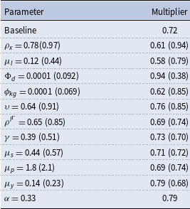
Finally, we conduct a sensitivity analysis. We typically examine how the fiscal multiplier changes when the value of one parameter is varied within the confidence intervals of its posterior estimates. For instance, the persistence of TFP is estimated to fall within the range of 0.78–0.97. Table 2 illustrates that the fiscal multiplier is 0.61 when persistence is at 0.78, and it increases to 0.94 when persistence reaches 0.97. As the persistence of TFP increases, changes in employment lead to more prolonged effects on TFP. With a persistence value of 0.97, changes in TFP become very persistent (hysteresis-like), leading to an increase in the multiplier. This result is identical to the findings of Engler and Tervala (Reference Engler and Tervala2018).
Sensitivity analysis

When the elasticity of TFP decreases, changes in employment cause a smaller impact on TFP, and the multiplier subsequently declines. This outcome is consistent with the findings of Engler and Tervala (Reference Engler and Tervala2018). When the elasticity of taxes with respect to public debt decreases, the tax rate hardly reacts to an increase in debt. Consequently, distortionary taxes do not rise in the short term, preventing adverse employment reactions to tax increases, thereby leading to an increase in the fiscal multiplier. The multiplier demonstrates considerable sensitivity to changes in the tax elasticity.
When productivity decreases (increases) to 0.001% (0.069%), the fiscal multiplier decreases (increases) to 0.62 (0.85). This outcome is well-established in previous research. Increasing the efficiency from 0.43 to 0.64 (the average in 20 emerging countries) raises the multiplier from 0.72 to 0.76. If efficiency reaches 0.91 (the average in G7 countries), the multiplier increases to 0.85. These results highlight the dependency on efficiency, aligning fully with Ganelli and Tervala (Reference Ganelli and Tervala2020). However, the magnitude of these changes underscores that merely enhancing efficiency alone cannot achieve miraculous results. When setting efficiency at 1 and productivity at 5%, akin to the parameters in Sims and Wolff (Reference Sims and Wolff2018), the multiplier reaches 1. This is close to the multiplier of 0.9 found by Sims and Wolff (Reference Sims and Wolff2018).
The multiplier remains unresponsive to changes in the duration of the public IS, the Calvo parameter, and the parameters of the monetary policy rule. Finally, reducing the output elasticity of private labor from 0.45 to 0.33 results in only a marginal increase in the fiscal multiplier. The sensitivity analysis indicates that the multiplier typically falls between 0.6 and 0.9, consistent with the IMF’s (2014) finding of a 0.5–0.9 range for multipliers in emerging economies.
6. Conclusions
The crucial role of public investment in China as a catalyst for economic growth and a primary instrument in stabilization policy is widely recognized. Berg et al. (Reference Berg, Buffie, Pattillo, Portillo, Presbitero and Zanna2019) argue in their theoretical study that when the efficiency of public investment is low, the resulting smaller stock of public capital has higher productivity, which compensates for the inefficiency. Therefore, in countries with low efficiency, increasing public investment can be beneficial, as the high productivity offsets the drawbacks of inefficiency.
Our study employs a Bayesian DSGE model that accounts for the inefficiency of public investment and enables the estimation of public capital productivity. We find that China faces a dual problem: both the efficiency of public investment and the productivity of public capital are remarkably low. The results directly contradict the theoretical findings of Berg et al. (Reference Berg, Buffie, Pattillo, Portillo, Presbitero and Zanna2019). When comparing the efficiency of public investment between China and other emerging economies, it is observed that China annually allocates 5.2% of its GDP to public investments that do not augment the capital stock. We estimate the output elasticity of public capital to be only 3%, compared to the 8% reported by Calderón et al. (Reference Calderón, Moral-Benito and Servén2015) for emerging economies. However, this estimate masks a higher elasticity of about 4% in the early years and a lower one of around 2% in the post-2008 sample, indicating a decline in the productivity of public capital over time.
This research provides macroeconomic support to the findings of Ansar et al. (Reference Ansar, Flyvbjerg, Budzier and Lunn2016), which suggest that China’s public investment scarcely creates economic value, and that China does not have a distinct advantage in their implementation. Low efficiency and productivity result in a modest fiscal multiplier (0.7). Our findings are consistent with empirical studies focusing on the impact of public investment in countries with low efficiency and emerging economies (IMF 2014). However, the fiscal multiplier for public investment in our model is approximately half that observed in advanced economies.
While Song et al. (Reference Song, Storesletten and Zilibotti2011) find that China has sustained high returns on investment despite significant capital accumulation, attributing these returns to the reallocation from low- to high-productivity firms, even amidst structural inefficiencies, particularly within SOEs, our research highlights the macroeconomic issues of public investments. We find that public investments yield low returns and create long-term economic challenges, presenting a more pessimistic view of China’s investment strategy. Lam and Moreno-Badia (Reference Lam and Moreno-Badia2023) similarly note a persistent decline in China’s public net financial worth since 2007, driven by rising local government debt, inefficiency in SOEs, and diminishing infrastructure returns. They argue that fiscal policies may have led to distortions, negatively impacting long-term TFP. Our findings support this, showing that China’s inefficient public investments contribute to reduced TFP, lower private investment, and a significant increase in the public debt-to-GDP ratio. A prudent economic policy would balance short-term stimulus with long-term fiscal sustainability, emphasizing the need to improve the efficiency and productivity of public investments.
Acknowledgements
We are grateful for the comments received from seminar participants at the Bank of Finland’s Institute for Economies in Transition (BOFIT), with special thanks to Zuzana Fungáčová, Risto Herrala, Riikka Nuutilainen, Iikka Korhonen, Michaela Elfsbacka Schmöller, and Matti Viren. We also thank an anonymous referee for valuable comments and suggestions that have significantly improved the paper.
Data availability
The data used in Figures 1 and 2 are available in the IMF’s investment and capital stock dataset (ICSD) at https://data.imf.org/?sk=1ce8a55f-cfa7-4bc0-bce2-256ee65ac0e4&sid=1441803350568. The data (real GDP, private consumption, private investment, public investment, and price level) used in Bayesian simulations is from “China’s Macroeconomy: Time Series Data” at https://www.atlantafed.org/cqer/research/china-macroeconomy and the quarterly average interest rate is derived from monthly data (discount rate for China) obtained from the Fred Economic Data at https://fred.stlouisfed.org/.

 Open access