
 K
K HNeKF2
 HNDKF2





1. Introduction
In equivariant stable homotopy theory, ordinary cohomology is represented by an equivariant Eilenberg–Mac Lane $G$
-spectrum
$G$
-spectrum $H\underline {M}$
, where
$H\underline {M}$
, where $\underline {M}$
is a Mackey functor for the group
$\underline {M}$
is a Mackey functor for the group $G$
. One may expect that the coefficients of an equivariant Eilenberg–Mac Lane spectrum are easy to understand, but this is more complicated than in the non-equivariant setting. The homotopy of a
$G$
. One may expect that the coefficients of an equivariant Eilenberg–Mac Lane spectrum are easy to understand, but this is more complicated than in the non-equivariant setting. The homotopy of a $G$
-spectrum
$G$
-spectrum $E$
can be considered as
$E$
can be considered as ${\textrm {RO}}(G)$
-graded, where
${\textrm {RO}}(G)$
-graded, where ${\textrm {RO}}(G)$
is the real representation ring of
${\textrm {RO}}(G)$
is the real representation ring of $G$
. In the case that
$G$
. In the case that $E=H\underline {M}$
for some
$E=H\underline {M}$
for some $G$
-Mackey functor
$G$
-Mackey functor $\underline {M}$
, the
$\underline {M}$
, the ${\textrm {RO}}(G)$
-graded coefficients of
${\textrm {RO}}(G)$
-graded coefficients of $E$
correspond to the Bredon homology of virtual real representation spheres of
$E$
correspond to the Bredon homology of virtual real representation spheres of $G$
with coefficients in
$G$
with coefficients in $\underline {M}$
.
$\underline {M}$
.
For $G=C_2$
, the
$G=C_2$
, the $RO(G)$
-graded coefficients of any equivariant Eilenberg–Mac Lane spectrum are quite well-understood [Reference Sikora18]. This is far from true for
$RO(G)$
-graded coefficients of any equivariant Eilenberg–Mac Lane spectrum are quite well-understood [Reference Sikora18]. This is far from true for $G = {\mathcal{K}} = C_2 \times C_2$
, the Klein-four group. One computational difficulty that arises in this context is that
$G = {\mathcal{K}} = C_2 \times C_2$
, the Klein-four group. One computational difficulty that arises in this context is that ${\textrm {RO}}({\mathcal{K}})$
is a free abelian group of rank four. Despite this, some computations of the
${\textrm {RO}}({\mathcal{K}})$
is a free abelian group of rank four. Despite this, some computations of the ${\textrm {RO}}({\mathcal{K}})$
-graded coefficients of
${\textrm {RO}}({\mathcal{K}})$
-graded coefficients of $H\underline {M}$
have been done [Reference Ellis-Bloor4, Reference Guillou and Yarnall5, Reference Holler and Kriz13, Reference Keyes15, Reference Slone19]. In this paper, we make further contributions to these computations. We compute a portion of the
$H\underline {M}$
have been done [Reference Ellis-Bloor4, Reference Guillou and Yarnall5, Reference Holler and Kriz13, Reference Keyes15, Reference Slone19]. In this paper, we make further contributions to these computations. We compute a portion of the ${\textrm {RO}}({\mathcal{K}})$
-graded homotopy Mackey functors of
${\textrm {RO}}({\mathcal{K}})$
-graded homotopy Mackey functors of $\underline {M} = N_H^{\mathcal{K}} \underline {{\mathbb{F}}_2}$
, where
$\underline {M} = N_H^{\mathcal{K}} \underline {{\mathbb{F}}_2}$
, where $H$
is a proper subgroup of
$H$
is a proper subgroup of $\mathcal{K}$
and
$\mathcal{K}$
and $\underline {{\mathbb{F}}_2}$
the constant
$\underline {{\mathbb{F}}_2}$
the constant $H$
-Mackey functor at
$H$
-Mackey functor at $\mathbb{F}_2$
. Here,
$\mathbb{F}_2$
. Here, $N_H^{\mathcal{K}}(\!-\!)\;:\; {\mathscr{M}\text{ack}}_H \rightarrow {\mathscr{M}\text{ack}}_{\mathcal{K}}$
is the Mackey functor norm. We also introduce a method for calculating the Mackey functors
$N_H^{\mathcal{K}}(\!-\!)\;:\; {\mathscr{M}\text{ack}}_H \rightarrow {\mathscr{M}\text{ack}}_{\mathcal{K}}$
is the Mackey functor norm. We also introduce a method for calculating the Mackey functors $N_H^G(\underline {{\mathbb{F}}_2})$
for any group
$N_H^G(\underline {{\mathbb{F}}_2})$
for any group $G$
and subgroup
$G$
and subgroup $H$
, based on Tambara ideals of the Burnside Tambara functor.
$H$
, based on Tambara ideals of the Burnside Tambara functor.
Hill, Hopkins and Ravenel introduced the norm functor $N_H^G(\!-\!)\;:\; \mathscr{S}\text{p}^H \rightarrow \mathscr{S}\text{p}^G$
in [Reference Hill, Hopkins and Ravenel9] and have studied various norms
$N_H^G(\!-\!)\;:\; \mathscr{S}\text{p}^H \rightarrow \mathscr{S}\text{p}^G$
in [Reference Hill, Hopkins and Ravenel9] and have studied various norms $N_{C_2}^G \textrm {BP}_{\mathbb{R}}$
, where
$N_{C_2}^G \textrm {BP}_{\mathbb{R}}$
, where $\textrm {BP}_{\mathbb{R}}$
is the Real Brown-Peterson
$\textrm {BP}_{\mathbb{R}}$
is the Real Brown-Peterson $C_2$
-spectrum. Despite the success of this analysis, many computations concerning equivariant spectra related to this norm construction remain mysterious. Along these lines, [Reference Meier, Shi and Zeng16, Theorem 4.4] gives partial information about the homotopy of the geometric fixed points
$C_2$
-spectrum. Despite the success of this analysis, many computations concerning equivariant spectra related to this norm construction remain mysterious. Along these lines, [Reference Meier, Shi and Zeng16, Theorem 4.4] gives partial information about the homotopy of the geometric fixed points $\Phi ^{C_2}N_{C_2}^{C_4} \textrm {BP}_{\mathbb{R}}\simeq N_e^{C_2} H{\mathbb{F}_2}$
. The first few
$\Phi ^{C_2}N_{C_2}^{C_4} \textrm {BP}_{\mathbb{R}}\simeq N_e^{C_2} H{\mathbb{F}_2}$
. The first few $\mathbb{Z}$
-graded homotopy Mackey functors are listed in Table 1 using notation as indicated in Table 3, and the
$\mathbb{Z}$
-graded homotopy Mackey functors are listed in Table 1 using notation as indicated in Table 3, and the $RO(C_2)$
-graded homotopy groups
$RO(C_2)$
-graded homotopy groups $\pi _{x+y\sigma } N_e^{C_2} H\mathbb{F}_2$
are displayed for
$\pi _{x+y\sigma } N_e^{C_2} H\mathbb{F}_2$
are displayed for $x\leq 6$
and
$x\leq 6$
and $x+y\leq 6$
in Figure 8. See the beginning of Section 7 for a discussion of Figure 8. A complete calculation of the homotopy of
$x+y\leq 6$
in Figure 8. See the beginning of Section 7 for a discussion of Figure 8. A complete calculation of the homotopy of $N_{C_2}^{C_4}\textrm {BP}_{\mathbb{R}}$
and
$N_{C_2}^{C_4}\textrm {BP}_{\mathbb{R}}$
and $N_e^{C_2} H \mathbb{F}_2$
is out of reach. Part of the reason for this is that the underlying homotopy groups of
$N_e^{C_2} H \mathbb{F}_2$
is out of reach. Part of the reason for this is that the underlying homotopy groups of $N_e^{C_2} H \mathbb{F}_2$
, together with the
$N_e^{C_2} H \mathbb{F}_2$
, together with the $C_2$
-action, form the dual Steenrod algebra with the action of the antipode. There is no known formula for the fixed points of this action. In contrast, the
$C_2$
-action, form the dual Steenrod algebra with the action of the antipode. There is no known formula for the fixed points of this action. In contrast, the ${\textrm {RO}}(C_2)$
-graded homotopy groups of both
${\textrm {RO}}(C_2)$
-graded homotopy groups of both $H_{C_2} N_e^{C_2} \mathbb{F}_2$
, the
$H_{C_2} N_e^{C_2} \mathbb{F}_2$
, the $0^{th}$
-Postnikov truncation of
$0^{th}$
-Postnikov truncation of $N_e^{C_2} H\mathbb{F}_2$
, and
$N_e^{C_2} H\mathbb{F}_2$
, and $H_{C_2} \underline {{\mathbb{F}}_2}$
are completely understood [Reference Dugger3, Reference Sikora18]. The
$H_{C_2} \underline {{\mathbb{F}}_2}$
are completely understood [Reference Dugger3, Reference Sikora18]. The $RO(C_2)$
-graded homotopy groups of the Eilenberg–Mac Lane spectra
$RO(C_2)$
-graded homotopy groups of the Eilenberg–Mac Lane spectra $H_{C_2} N_e^{C_2} \mathbb{F}_2$
and
$H_{C_2} N_e^{C_2} \mathbb{F}_2$
and $H_{C_2} \underline {\mathbb{F}}_2$
are displayed in Figures 6 and 7, respectively.
$H_{C_2} \underline {\mathbb{F}}_2$
are displayed in Figures 6 and 7, respectively.
The homotopy Mackey functors $\underline \pi _n N_e^{C_2} H \mathbb{F}_2$
,
$\underline \pi _n N_e^{C_2} H \mathbb{F}_2$
, $n\leq 6$
. See Table 3for the Mackey functor Lewis diagrams
$n\leq 6$
. See Table 3for the Mackey functor Lewis diagrams

Motivation for the study of $N_{C_2}^{C_4}\textrm {BP}_{\mathbb{R}}$
comes from chromatic homotopy theory [Reference Hill, Shi, Wang and Xu12]. The quaternion group
$N_{C_2}^{C_4}\textrm {BP}_{\mathbb{R}}$
comes from chromatic homotopy theory [Reference Hill, Shi, Wang and Xu12]. The quaternion group $Q_8$
also plays an important role in chromatic homotopy theory, which suggests the study of
$Q_8$
also plays an important role in chromatic homotopy theory, which suggests the study of $N_{C_2}^{Q_8} \textrm {BP}_{\mathbb{R}}$
, where
$N_{C_2}^{Q_8} \textrm {BP}_{\mathbb{R}}$
, where $C_2$
is the centre of
$C_2$
is the centre of $Q_8$
. This is expected to be difficult; however, given that the quotient
$Q_8$
. This is expected to be difficult; however, given that the quotient $Q_8/C_2$
is isomorphic to
$Q_8/C_2$
is isomorphic to $\mathcal{K}$
, one may wish to compute
$\mathcal{K}$
, one may wish to compute $\Phi ^{C_2}N_{C_2}^{Q_8} \textrm {BP}_{\mathbb{R}} \simeq N_e^{{\mathcal{K}}} H\mathbb{F}_2$
. Again, this is out of reach, though its Postnikov truncation
$\Phi ^{C_2}N_{C_2}^{Q_8} \textrm {BP}_{\mathbb{R}} \simeq N_e^{{\mathcal{K}}} H\mathbb{F}_2$
. Again, this is out of reach, though its Postnikov truncation $H_{\mathcal{K}} N_e^{\mathcal{K}} \mathbb{F}_2$
can be completely computed. The
$H_{\mathcal{K}} N_e^{\mathcal{K}} \mathbb{F}_2$
can be completely computed. The $RO({\mathcal{K}})$
-graded homotopy groups of
$RO({\mathcal{K}})$
-graded homotopy groups of $H\underline {{\mathbb{F}}_2}$
were previously computed in [Reference Ellis-Bloor4, Reference Holler and Kriz13], while some of the homotopy Mackey functors were determined in [Reference Guillou and Yarnall5]. These are depicted in a range in Figure 9. In this article, we compute a portion of the
$H\underline {{\mathbb{F}}_2}$
were previously computed in [Reference Ellis-Bloor4, Reference Holler and Kriz13], while some of the homotopy Mackey functors were determined in [Reference Guillou and Yarnall5]. These are depicted in a range in Figure 9. In this article, we compute a portion of the ${\textrm {RO}}({\mathcal{K}})$
-graded homotopy Mackey functors of
${\textrm {RO}}({\mathcal{K}})$
-graded homotopy Mackey functors of $H_{\mathcal{K}} N_e^{{\mathcal{K}}} {\mathbb{F}_2}$
. It is common to use the symbol
$H_{\mathcal{K}} N_e^{{\mathcal{K}}} {\mathbb{F}_2}$
. It is common to use the symbol $\bigstar$
to denote a grading over
$\bigstar$
to denote a grading over $RO(G)$
. We will use the symbol
$RO(G)$
. We will use the symbol $\blacklozenge$
to denote a grading over the
$\blacklozenge$
to denote a grading over the $\mathrm{Aut}({\mathcal{K}})$
-fixed subgroup
$\mathrm{Aut}({\mathcal{K}})$
-fixed subgroup $\mathbb{Z}\{1,\overline {\rho }\}\subset RO({\mathcal{K}})$
, where
$\mathbb{Z}\{1,\overline {\rho }\}\subset RO({\mathcal{K}})$
, where $\overline {\rho }$
is the reduced regular representation.
$\overline {\rho }$
is the reduced regular representation.
Theorem A.
The homotopy Mackey functors $\underline {\pi }_{\blacklozenge }H_{\mathcal{K}} N_e^{\mathcal{K}} \mathbb{F}_2$
are as described in Section
4
and displayed in Figures 11 and 12
, where
$\underline {\pi }_{\blacklozenge }H_{\mathcal{K}} N_e^{\mathcal{K}} \mathbb{F}_2$
are as described in Section
4
and displayed in Figures 11 and 12
, where $\blacklozenge \in \mathbb{Z}\{1,\overline {\rho }\}\subset RO({\mathcal{K}})$
.
$\blacklozenge \in \mathbb{Z}\{1,\overline {\rho }\}\subset RO({\mathcal{K}})$
.
In particular, the quotient map $ N_e^{\mathcal{K}} \mathbb{F}_2 \rightarrow \underline {{\mathbb{F}}_2}$
induces an isomorphism
$ N_e^{\mathcal{K}} \mathbb{F}_2 \rightarrow \underline {{\mathbb{F}}_2}$
induces an isomorphism
 \begin{equation*} \underline {\pi }_{n+k\overline {\rho }}\big(HN_e^{\mathcal{K}} \mathbb{F}_2\big) \rightarrow \underline {\pi }_{n+k\overline {\rho }}(H\underline {{\mathbb{F}}_2}) \end{equation*}
in a subrange of each of the positive and negative cones. These subranges are above the line through $(3,-1)$
with slope
$(3,-1)$
with slope $-1$
and below the line through
$-1$
and below the line through $(\!-\!2,1)$
with slope
$(\!-\!2,1)$
with slope $-1$
, respectively.
$-1$
, respectively.
We also consider the intermediate norm $N_C^{\mathcal{K}} \underline {{\mathbb{F}}_2}$
, where
$N_C^{\mathcal{K}} \underline {{\mathbb{F}}_2}$
, where $C\leq K$
is an order 2 subgroup. The corresponding Eilenberg–Mac Lane spectrum
$C\leq K$
is an order 2 subgroup. The corresponding Eilenberg–Mac Lane spectrum $H_{\mathcal{K}} N_C^{\mathcal{K}} \underline {{\mathbb{F}}_2}$
is the Postnikov truncation of the normed spectrum
$H_{\mathcal{K}} N_C^{\mathcal{K}} \underline {{\mathbb{F}}_2}$
is the Postnikov truncation of the normed spectrum $N_C^{\mathcal{K}} H_C \underline {{\mathbb{F}}_2}$
. The latter is a useful intermediary between the mysterious
$N_C^{\mathcal{K}} H_C \underline {{\mathbb{F}}_2}$
. The latter is a useful intermediary between the mysterious $N_e^{\mathcal{K}} H\mathbb{F}_2$
and the well-understood
$N_e^{\mathcal{K}} H\mathbb{F}_2$
and the well-understood $H_{\mathcal{K}} \underline {{\mathbb{F}}_2}$
, in that
$H_{\mathcal{K}} \underline {{\mathbb{F}}_2}$
, in that $H_{\mathcal{K}}\underline {{\mathbb{F}}_2} = N_{\mathcal{K}}^{\mathcal{K}} H_{\mathcal{K}}\underline {{\mathbb{F}}_2}$
. For definiteness, we specialize to the case that
$H_{\mathcal{K}}\underline {{\mathbb{F}}_2} = N_{\mathcal{K}}^{\mathcal{K}} H_{\mathcal{K}}\underline {{\mathbb{F}}_2}$
. For definiteness, we specialize to the case that $C=D$
is the diagonal subgroup of
$C=D$
is the diagonal subgroup of $\mathcal{K}$
, though the other choices can be obtained by using the
$\mathcal{K}$
, though the other choices can be obtained by using the $\mathrm{Aut}({\mathcal{K}})$
-action.
$\mathrm{Aut}({\mathcal{K}})$
-action.
Theorem B.
The homotopy Mackey functors $\underline {\pi }_{\blacklozenge }H_{\mathcal{K}} N_D^{\mathcal{K}} \underline {{\mathbb{F}}_2}$
are as described in Section 5 and displayed in Figures 13 and 14, where
$\underline {\pi }_{\blacklozenge }H_{\mathcal{K}} N_D^{\mathcal{K}} \underline {{\mathbb{F}}_2}$
are as described in Section 5 and displayed in Figures 13 and 14, where $\blacklozenge \in \mathbb{Z}\{1,\overline {\rho }\}\subset RO({\mathcal{K}})$
.
$\blacklozenge \in \mathbb{Z}\{1,\overline {\rho }\}\subset RO({\mathcal{K}})$
.
As in Theorem
A
, the quotient map $ N_D^{\mathcal{K}} \underline {{\mathbb{F}}_2} \rightarrow \underline {{\mathbb{F}}_2}$
induces an isomorphism
$ N_D^{\mathcal{K}} \underline {{\mathbb{F}}_2} \rightarrow \underline {{\mathbb{F}}_2}$
induces an isomorphism
 \begin{equation*} \underline {\pi }_{n+k\overline {\rho }}\big(HN_D^{\mathcal{K}} \underline {{\mathbb{F}}_2}\big) \rightarrow \underline {\pi }_{n+k\overline {\rho }}(H\underline {{\mathbb{F}}_2}) \end{equation*}
in a subrange of each of the positive and negative cones. These subranges are above the line through $(3,-1)$
with slope
$(3,-1)$
with slope $-1$
and below the line through
$-1$
and below the line through $(\!-\!2,1)$
with slope
$(\!-\!2,1)$
with slope $-1$
, respectively.
$-1$
, respectively.
1.1. Conventions
We write $e$
for a trivial group and
$e$
for a trivial group and $C_2 \;:\!=\; \langle \gamma \mid \gamma ^2 = 1 \rangle$
for a finite group of order two. Our main group of interest is the Klein four-group
$C_2 \;:\!=\; \langle \gamma \mid \gamma ^2 = 1 \rangle$
for a finite group of order two. Our main group of interest is the Klein four-group ${\mathcal{K}} \;:\!=\; C_2 \times C_2$
; its nontrivial subgroups are
${\mathcal{K}} \;:\!=\; C_2 \times C_2$
; its nontrivial subgroups are $L \;:\!=\; C_2 \times e$
,
$L \;:\!=\; C_2 \times e$
, $D \;:\!=\; \langle (\gamma , \gamma ) \rangle$
, and
$D \;:\!=\; \langle (\gamma , \gamma ) \rangle$
, and $R \;:\!=\; e \times C_2$
.
$R \;:\!=\; e \times C_2$
.
We write both $\mathbb{Z}/2$
and
$\mathbb{Z}/2$
and $\mathbb{F}_2$
for the ring of order 2, guided by aesthetics.
$\mathbb{F}_2$
for the ring of order 2, guided by aesthetics.
We use different fonts to differentiate between non-equivariant, $C_2$
-equivariant, and
$C_2$
-equivariant, and $\mathcal{K}$
-equivariant homotopy theory. We write
$\mathcal{K}$
-equivariant homotopy theory. We write $\textrm {H}$
for non-equivariant Eilenberg–Mac Lane spectra,
$\textrm {H}$
for non-equivariant Eilenberg–Mac Lane spectra, $\mathbf{H}$
for
$\mathbf{H}$
for $C_2$
-equivariant Eilenberg–Mac Lane spectra, and
$C_2$
-equivariant Eilenberg–Mac Lane spectra, and $\boldsymbol{\mathscr{H}}$
for
$\boldsymbol{\mathscr{H}}$
for $\mathcal{K}$
-equivariant Eilenberg–Mac Lane spectra. Similarly, we will often abbreviate the Mackey functors
$\mathcal{K}$
-equivariant Eilenberg–Mac Lane spectra. Similarly, we will often abbreviate the Mackey functors $N_e^{C_2} \mathbb{F}_2, N_e^{\mathcal{K}} \mathbb{F}_2,$
and
$N_e^{C_2} \mathbb{F}_2, N_e^{\mathcal{K}} \mathbb{F}_2,$
and $ N_D^{\mathcal{K}} \underline {{\mathbb{F}}_2}$
by
$ N_D^{\mathcal{K}} \underline {{\mathbb{F}}_2}$
by $\mathbf{N}, \boldsymbol{\mathscr{N}},$
and
$\mathbf{N}, \boldsymbol{\mathscr{N}},$
and $\boldsymbol{\mathscr{N}}_{\!D}$
, respectively.
$\boldsymbol{\mathscr{N}}_{\!D}$
, respectively.
Equivariant spectra will always be considered as indexed over a complete universe, so that their homotopy is valued in Mackey functors. Our calculations require many $C_2$
- or
$C_2$
- or $\mathcal{K}$
-Mackey functors; notation and definition for these can be found in Tables 3 and 4.
$\mathcal{K}$
-Mackey functors; notation and definition for these can be found in Tables 3 and 4.
2. $\mathcal{K}$
-norms via Tambara ideals
$\mathcal{K}$
-norms via Tambara ideals

The Hill–Hopkins–Ravenel norm $N_H^G \colon \mathscr{S}\text{p}^H \to \mathscr{S}\text{p}^G$
is captured on the level of Mackey functors by a functor
$N_H^G \colon \mathscr{S}\text{p}^H \to \mathscr{S}\text{p}^G$
is captured on the level of Mackey functors by a functor $N_H^{G} \colon {\mathscr{M}\text{ack}}(H) \to {\mathscr{M}\text{ack}}(G)$
. As a non-additive functor between additive categories, the norm is often difficult to compute. We introduce a technique for computing
$N_H^{G} \colon {\mathscr{M}\text{ack}}(H) \to {\mathscr{M}\text{ack}}(G)$
. As a non-additive functor between additive categories, the norm is often difficult to compute. We introduce a technique for computing $N_H^G(\underline {{\mathbb{F}}_2})$
based on Tambara ideals and use it to compute
$N_H^G(\underline {{\mathbb{F}}_2})$
based on Tambara ideals and use it to compute $N_e^{\mathcal{K}}(\mathbb{F}_2)$
and
$N_e^{\mathcal{K}}(\mathbb{F}_2)$
and $N_C^{\mathcal{K}}(\underline {{\mathbb{F}}_2})$
, where
$N_C^{\mathcal{K}}(\underline {{\mathbb{F}}_2})$
, where $C$
is any of the order two subgroups of
$C$
is any of the order two subgroups of $\mathcal{K}$
.
$\mathcal{K}$
.
2.1. Norms of Mackey and Tambara functors
Recall that the category of $G$
-Mackey functors is the category of additive functors
$G$
-Mackey functors is the category of additive functors $\mathcal{A}_G \to {\mathscr{A}\text{b}}$
, where
$\mathcal{A}_G \to {\mathscr{A}\text{b}}$
, where $\mathcal{A}_G$
is the Burnside category for
$\mathcal{A}_G$
is the Burnside category for $G$
.
$G$
.
Definition 2.1 ([Reference Hoyer14], Definition 2.3.2). The functor $N_H^G \colon {\mathscr{M}\text{ack}}(H) \to {\mathscr{M}\text{ack}}(G)$
is given by left Kan extension along coinduction
$N_H^G \colon {\mathscr{M}\text{ack}}(H) \to {\mathscr{M}\text{ack}}(G)$
is given by left Kan extension along coinduction ${\mathscr{F}\text{in}}_H(G,-) \colon \mathcal{A}_H \to \mathcal{A}_G$
.
${\mathscr{F}\text{in}}_H(G,-) \colon \mathcal{A}_H \to \mathcal{A}_G$
.
Tambara functors are the $G$
-commutative monoids in the category of
$G$
-commutative monoids in the category of $G$
-Mackey functors. Alternatively, the category of
$G$
-Mackey functors. Alternatively, the category of $G$
-Tambara functors is the category of product preserving functors
$G$
-Tambara functors is the category of product preserving functors $\underline {T} \colon \mathcal{P}^G \to {\mathscr{S}\text{et}}$
such that each
$\underline {T} \colon \mathcal{P}^G \to {\mathscr{S}\text{et}}$
such that each $\underline {T}(U)$
is a commutative ring, where
$\underline {T}(U)$
is a commutative ring, where $\mathcal{P}^G$
is the category of polynomials of finite
$\mathcal{P}^G$
is the category of polynomials of finite $G$
-sets [Reference Tambara20, Section 8]. Concretely, a Tambara functor is a Mackey functor valued in commutative rings whose restrictions are ring homomorphisms satisfying Frobenius reciprocity (a Green functor) equipped with norm maps (of multiplicative monoids) satisfying Tambara reciprocity.
$G$
-sets [Reference Tambara20, Section 8]. Concretely, a Tambara functor is a Mackey functor valued in commutative rings whose restrictions are ring homomorphisms satisfying Frobenius reciprocity (a Green functor) equipped with norm maps (of multiplicative monoids) satisfying Tambara reciprocity.
The norm $n_H^G$
from
$n_H^G$
from $H$
-Tambara functors to
$H$
-Tambara functors to $G$
-Tambara functors is slightly different from the norm of Mackey functors.
$G$
-Tambara functors is slightly different from the norm of Mackey functors.
Definition 2.2 ([Reference Blumberg and Hill2], Definition 6.8, Proposition 6.9). The functor $n_H^G \colon {\mathscr{T}\text{amb}}(H) \to {\mathscr{T}\text{amb}}(G)$
is given by left Kan extension along the inclusion
$n_H^G \colon {\mathscr{T}\text{amb}}(H) \to {\mathscr{T}\text{amb}}(G)$
is given by left Kan extension along the inclusion $\mathcal{P}^H \to \mathcal{P}^G$
; it is left adjoint to the restriction functor
$\mathcal{P}^H \to \mathcal{P}^G$
; it is left adjoint to the restriction functor $\textrm {res}^G_H \colon {\mathscr{T}\text{amb}}(G) \to {\mathscr{T}\text{amb}}(H)$
.
$\textrm {res}^G_H \colon {\mathscr{T}\text{amb}}(G) \to {\mathscr{T}\text{amb}}(H)$
.
We recall a theorem relating the two functors:
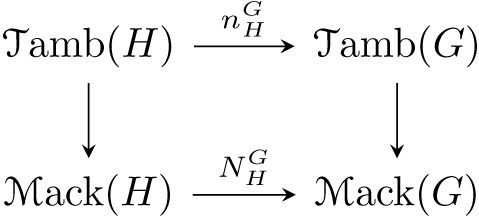
Theorem 2.3 ([Reference Hoyer14], Theorem 2.3.3). The following square commutes, where vertical arrows are forgetful functors:
2.2. Tambara ideals and norms
Like commutative rings, Tambara functors have a robust theory of ideals. We use non-unital Tambara functors to define Tambara ideals.
Let ${\mathscr{E}\text{pi}}^G \subseteq {\mathscr{F}\text{in}}^G$
be the category of finite
${\mathscr{E}\text{pi}}^G \subseteq {\mathscr{F}\text{in}}^G$
be the category of finite $G$
-sets and surjections. Note that
$G$
-sets and surjections. Note that ${\mathscr{E}\text{pi}}^G$
is a pullback stable subcategory of finite
${\mathscr{E}\text{pi}}^G$
is a pullback stable subcategory of finite $G$
-sets, that is pullbacks in
$G$
-sets, that is pullbacks in ${\mathscr{F}\text{in}}^G$
of morphisms in
${\mathscr{F}\text{in}}^G$
of morphisms in ${\mathscr{E}\text{pi}}^G$
are again in
${\mathscr{E}\text{pi}}^G$
are again in ${\mathscr{E}\text{pi}}^G$
. Let
${\mathscr{E}\text{pi}}^G$
. Let $\mathcal{P}^G_{\mathscr{E}\text{pi}}$
be the category of polynomials with exponents in
$\mathcal{P}^G_{\mathscr{E}\text{pi}}$
be the category of polynomials with exponents in ${\mathscr{E}\text{pi}}^G$
[Reference Blumberg and Hill2, Definition 2.7].
${\mathscr{E}\text{pi}}^G$
[Reference Blumberg and Hill2, Definition 2.7].
Definition 2.4 ([Reference Blumberg and Hill2], Definition 4.15). A non-unital Tambara functor is a product preserving functor $\underline {T} \colon \mathcal{P}^G_{\mathscr{E}\text{pi}} \to {\mathscr{S}\text{et}}$
such that each
$\underline {T} \colon \mathcal{P}^G_{\mathscr{E}\text{pi}} \to {\mathscr{S}\text{et}}$
such that each $\underline {T}(X)$
is an abelian group.
$\underline {T}(X)$
is an abelian group.
Concretely, a non-unital Tambara functor is a Tambara functor valued in non-unital rings, that is, a Mackey functor valued in non-unital commutative rings whose restrictions are ring homomorphisms satisfying Frobenius reciprocity (a non-unital Green functor) equipped with norm maps (of non-unital multiplicative monoids) satisfying Tambara reciprocity.
The definition below is equivalent to the original definition given by Nakaoka [Reference Nakaoka17, Definition 2.1].
Definition 2.5 ([Reference Hill7], sentence before definition 5.1). A Tambara ideal $\underline {I}$
of a Tambara functor
$\underline {I}$
of a Tambara functor $\underline {T}$
is a sub-non-unital Tambara functor of
$\underline {T}$
is a sub-non-unital Tambara functor of $\underline {T}$
with a morphism of non-unital Tambara functors
$\underline {T}$
with a morphism of non-unital Tambara functors $\underline {T} \boxtimes \underline {I} \to \underline {I}$
.
$\underline {T} \boxtimes \underline {I} \to \underline {I}$
.
Practically speaking, a Tambara ideal $\underline {I}$
of a Tambara functor
$\underline {I}$
of a Tambara functor $\underline {T}$
is a collection of ideals
$\underline {T}$
is a collection of ideals $\underline {I}(G/H) \subseteq \underline {T}(G/H)$
closed under restriction, transfer, and norm.
$\underline {I}(G/H) \subseteq \underline {T}(G/H)$
closed under restriction, transfer, and norm.
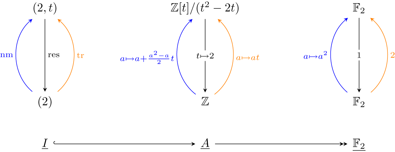
Example 2.6.
Recall that the Burnside ring for $C_2$
is
$C_2$
is
 \begin{equation*} A(C_2) \cong \displaystyle \mathchoice {{\mathbb{Z}[t]}\big /\!{(t^2-2t),}} {{}^{\mathbb{Z}[t]}\!/_{\!(t^2-2t),}}{ \mathbb{Z}[t] / (t^2-2t),}{ \mathbb{Z}[t] / (t^2-2t),} \end{equation*}
where $t = [{}^{C_2}\!/_{\!e}]$
. Let
$t = [{}^{C_2}\!/_{\!e}]$
. Let $\underline {I}$
be the Tambara ideal generated by
$\underline {I}$
be the Tambara ideal generated by $2 \in \underline {A}(C_2/C_2)$
inside the
$2 \in \underline {A}(C_2/C_2)$
inside the $C_2$
-Burnside Tambara functor
$C_2$
-Burnside Tambara functor $\underline {A}$
. This is the smallest Tambara ideal of
$\underline {A}$
. This is the smallest Tambara ideal of $\underline {A}$
containing
$\underline {A}$
containing $2 \in \underline {A}(C_2/C_2)$
. This ideal must contain
$2 \in \underline {A}(C_2/C_2)$
. This ideal must contain
 \begin{equation*} 2 = {\textrm {res}}(2) \in \underline {A}(C_2/e) \end{equation*}
at the underlying level and
 \begin{equation*} 2t = {\textrm {tr}}{\textrm {res}}(2),\quad 2 + t = \textrm {nm}\;\textrm {res}(2) \in \underline {A}(C_2/C_2) \end{equation*}
at the fixed level. Altogether, a minimal generating set for $\underline {I}(C_2/C_2)$
is
$\underline {I}(C_2/C_2)$
is $(2,t)$
and a minimal generating set for
$(2,t)$
and a minimal generating set for $\underline {I}(C_2/e)$
is
$\underline {I}(C_2/e)$
is $(2)$
. The quotient Tambara functor
$(2)$
. The quotient Tambara functor $\underline {A}/\underline {I}$
is therefore isomorphic to
$\underline {A}/\underline {I}$
is therefore isomorphic to $\underline {{\mathbb{F}}_2}$
.
$\underline {{\mathbb{F}}_2}$
.
It is often the case that many Mackey functors of interest can be written as quotients of the Burnside Tambara functor. For instance, the previous example shows that $\underline {{\mathbb{F}}_2}$
is a quotient of
$\underline {{\mathbb{F}}_2}$
is a quotient of $\underline {A}$
, and
$\underline {A}$
, and $\underline {\mathbb{Z}}$
is a quotient of
$\underline {\mathbb{Z}}$
is a quotient of $\underline {A}$
by the Tambara ideal generated by
$\underline {A}$
by the Tambara ideal generated by $t-2 \in \underline {A}(C_2/C_2)$
. Writing
$t-2 \in \underline {A}(C_2/C_2)$
. Writing $\underline {{\mathbb{F}}_2}$
as the quotient of
$\underline {{\mathbb{F}}_2}$
as the quotient of $\underline {A}$
by this Tambara ideal is a productive strategy to compute its norms.
$\underline {A}$
by this Tambara ideal is a productive strategy to compute its norms.
Proposition 2.7.
Let $G$
be a group which contains a subgroup isomorphic to
$G$
be a group which contains a subgroup isomorphic to $C_2$
. The norm
$C_2$
. The norm $n_{C_2}^G(\underline {{\mathbb{F}}_2})$
is the quotient of the
$n_{C_2}^G(\underline {{\mathbb{F}}_2})$
is the quotient of the $G$
-Burnside Tambara functor
$G$
-Burnside Tambara functor $\underline {A}$
by the Tambara ideal generated by
$\underline {A}$
by the Tambara ideal generated by $2 \in \underline {A}(G/{C_2})$
.
$2 \in \underline {A}(G/{C_2})$
.
Proof.
The $C_2$
-Tambara ideal
$C_2$
-Tambara ideal $\underline {I} \subseteq \underline {A}$
generated by
$\underline {I} \subseteq \underline {A}$
generated by $2 \in \underline {A}({C_2}/{C_2})$
is the image of the
$2 \in \underline {A}({C_2}/{C_2})$
is the image of the $C_2$
-Tambara functor homomorphism
$C_2$
-Tambara functor homomorphism $\underline {A}[x_{{C_2}/{C_2}}] \to \underline {A}$
determined by
$\underline {A}[x_{{C_2}/{C_2}}] \to \underline {A}$
determined by $x \mapsto 2$
, where
$x \mapsto 2$
, where $\underline {A}[x_{{C_2}/{C_2}}]$
is the free
$\underline {A}[x_{{C_2}/{C_2}}]$
is the free $H$
-Tambara functor generated at the top level [Reference Blumberg and Hill2, Definition 5.4].
$H$
-Tambara functor generated at the top level [Reference Blumberg and Hill2, Definition 5.4].
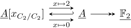
We may therefore write the $C_2$
-Tambara functor
$C_2$
-Tambara functor $\underline {{\mathbb{F}}_2}$
as a reflexive coequalizer in the category
$\underline {{\mathbb{F}}_2}$
as a reflexive coequalizer in the category ${\mathscr{T}\text{amb}}({C_2})$
:
${\mathscr{T}\text{amb}}({C_2})$
:
Since $n_{{C_2}}^G \colon {\mathscr{T}\text{amb}}({C_2}) \to {\mathscr{T}\text{amb}}(G)$
is a left adjoint, it preserves coequalizers. The Tambara norm
$n_{{C_2}}^G \colon {\mathscr{T}\text{amb}}({C_2}) \to {\mathscr{T}\text{amb}}(G)$
is a left adjoint, it preserves coequalizers. The Tambara norm $n_{{C_2}}^G$
sends the
$n_{{C_2}}^G$
sends the $C_2$
-Burnside functor to the
$C_2$
-Burnside functor to the $G$
-Burnside functor. By [Reference Hill, Mehrle and Quigley11, Proposition 4.2], we know that
$G$
-Burnside functor. By [Reference Hill, Mehrle and Quigley11, Proposition 4.2], we know that $n_{{C_2}}^G(\underline {A}[x_{{C_2}/{C_2}}])$
is isomorphic to
$n_{{C_2}}^G(\underline {A}[x_{{C_2}/{C_2}}])$
is isomorphic to $\underline {A}[x_{G/{C_2}}]$
. Thus, we have a reflexive coequalizer in
$\underline {A}[x_{G/{C_2}}]$
. Thus, we have a reflexive coequalizer in ${\mathscr{T}\text{amb}}(G)$
:
${\mathscr{T}\text{amb}}(G)$
:

This expresses $n_{{C_2}}^G(\underline {{\mathbb{F}}_2})$
as the quotient of the
$n_{{C_2}}^G(\underline {{\mathbb{F}}_2})$
as the quotient of the $G$
-Tambara functor
$G$
-Tambara functor $\underline {A}$
by the ideal generated by
$\underline {A}$
by the ideal generated by $2 \in \underline {A}(G/{C_2})$
.
$2 \in \underline {A}(G/{C_2})$
.
Although the proposition above is stated for the norm from $C_2$
to
$C_2$
to $G$
, a similar strategy works to calculate other norms, as the following example shows.
$G$
, a similar strategy works to calculate other norms, as the following example shows.
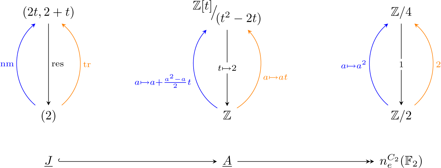
Example 2.8. $n_e^{C_2}(\mathbb{F}_2) \cong \underline {A}/\underline {J}$
, where
$n_e^{C_2}(\mathbb{F}_2) \cong \underline {A}/\underline {J}$
, where $\underline {J}$
is the Tambara ideal of
$\underline {J}$
is the Tambara ideal of $\underline {A}$
generated by
$\underline {A}$
generated by $2 \in \underline {A}(C_2/e)$
. At the fixed level, minimal generators for this ideal are
$2 \in \underline {A}(C_2/e)$
. At the fixed level, minimal generators for this ideal are $(2t, 2+t)$
.
$(2t, 2+t)$
.
Remark 2.9.
If $\underline {I}$
is a Tambara ideal of a Tambara functor
$\underline {I}$
is a Tambara ideal of a Tambara functor $\underline {T}$
, we might expect a statement like the following to be true:
$\underline {T}$
, we might expect a statement like the following to be true: $N_H^G(\underline {I})$
is a Tambara ideal of
$N_H^G(\underline {I})$
is a Tambara ideal of $n_H^G(\underline {T})$
, and the norm of the quotient
$n_H^G(\underline {T})$
, and the norm of the quotient $n_H^G(\underline {T}/\underline {I})$
is the quotient of the norm
$n_H^G(\underline {T}/\underline {I})$
is the quotient of the norm $n_H^G(\underline {T}) / N_H^G(\underline {I})$
. There are several obstacles to making this statement precise. Although
$n_H^G(\underline {T}) / N_H^G(\underline {I})$
. There are several obstacles to making this statement precise. Although $N_H^G \colon {\mathscr{M}\text{ack}}(H) \to {\mathscr{M}\text{ack}}(G)$
is a left adjoint, it is not an exact functor (nor even additive). Furthermore,
$N_H^G \colon {\mathscr{M}\text{ack}}(H) \to {\mathscr{M}\text{ack}}(G)$
is a left adjoint, it is not an exact functor (nor even additive). Furthermore, $\underline {T}/\underline {I}$
is not a colimit in
$\underline {T}/\underline {I}$
is not a colimit in $H$
-Tambara functors, and there’s no reason it should be preserved by
$H$
-Tambara functors, and there’s no reason it should be preserved by $n_H^G$
.
$n_H^G$
.
2.3.
The norm
$N_e^{\mathcal{K}}(\mathbb{F}_2)$

Recall that the Burnside ring for $\mathcal{K}$
is
$\mathcal{K}$
is
 \begin{equation*} A({\mathcal{K}}) \cong \displaystyle \mathchoice {{\mathbb{Z}[t_L,t_D,t_R]}\big /\!{t_Lt_D = t_Lt_R = t_Dt_R, t_\bullet ^2 = 2t_\bullet ,}} {{}^{\mathbb{Z}[t_L,t_D,t_R]}\!/_{\!t_Lt_D = t_Lt_R = t_Dt_R, t_\bullet ^2 = 2t_\bullet ,}}{ \mathbb{Z}[t_L,t_D,t_R] / t_Lt_D = t_Lt_R = t_Dt_R, t_\bullet ^2 = 2t_\bullet ,}{ \mathbb{Z}[t_L,t_D,t_R] / t_Lt_D = t_Lt_R = t_Dt_R, t_\bullet ^2 = 2t_\bullet ,} \end{equation*}
where $t_L = [{}^{{\mathcal{K}}}\!/_{\!L}]$
,
$t_L = [{}^{{\mathcal{K}}}\!/_{\!L}]$
, $t_D = [{}^{{\mathcal{K}}}\!/_{\!D}]$
and
$t_D = [{}^{{\mathcal{K}}}\!/_{\!D}]$
and $t_R = [{}^{{\mathcal{K}}}\!/_{\!R}]$
. The relation
$t_R = [{}^{{\mathcal{K}}}\!/_{\!R}]$
. The relation $t_\bullet ^2 = 2t_\bullet$
holds for all
$t_\bullet ^2 = 2t_\bullet$
holds for all $\bullet \in \{L,D,R\}$
. Note that the class
$\bullet \in \{L,D,R\}$
. Note that the class $[{}^{{\mathcal{K}}}\!/_{\!e}]$
is unnecessary as a generator, since
$[{}^{{\mathcal{K}}}\!/_{\!e}]$
is unnecessary as a generator, since $[{}^{{\mathcal{K}}}\!/_{\!e}] = t_Lt_D = t_Lt_R = t_Dt_R$
. The Burnside Tambara functor
$[{}^{{\mathcal{K}}}\!/_{\!e}] = t_Lt_D = t_Lt_R = t_Dt_R$
. The Burnside Tambara functor $\underline {A}$
for the Klein four-group is displayed in Figure 1. In the Tambara functor
$\underline {A}$
for the Klein four-group is displayed in Figure 1. In the Tambara functor $\underline {A}$
, the norm
$\underline {A}$
, the norm $\textrm {nm}_e^L$
is given by
$\textrm {nm}_e^L$
is given by
 \begin{equation*} \textrm {nm}_e^L(a) = a + \left (\tfrac {a^2 - a}{2}\right ) s_L, \end{equation*}
and the norm $\textrm {nm}_L^{\mathcal{K}}$
is given by
$\textrm {nm}_L^{\mathcal{K}}$
is given by
 \begin{equation*} \textrm {nm}_L^{\mathcal{K}}(a\,s_L + b)\ =\ \left (a^2-a+ba \right )t_Dt_R \, + \, \left (\tfrac {b^2-b}{2}\right )t_L \, + \, a\,t_D \, + \, a\, t_R + b, \end{equation*}
and similarly for norms to or from $D$
and
$D$
and $R$
.
$R$
.
The Burnside $\mathcal{K}$
-Tambara functor
$\mathcal{K}$
-Tambara functor $\underline {A}$
.
$\underline {A}$
.

Proposition 2.10.
The value of the $\mathcal{K}$
-Tambara functor
$\mathcal{K}$
-Tambara functor $n_e^{\mathcal{K}}(\mathbb{F}_2)$
at the trivial orbit
$n_e^{\mathcal{K}}(\mathbb{F}_2)$
at the trivial orbit ${\mathcal{K}}/{\mathcal{K}}$
is the ring
${\mathcal{K}}/{\mathcal{K}}$
is the ring
 \begin{equation*} n_e^{\mathcal{K}}(\mathbb{F}_2)({\mathcal{K}}/{\mathcal{K}}) \cong \displaystyle \mathchoice {{\mathbb{Z}/8[b_L,b_R]}\big /\!{(2b_Lb_R,2b_R,b_L^2,b_R^2,b_Lb_R)}} {{}^{\mathbb{Z}/8[b_L,b_R]}\!/_{\!(2b_Lb_R,2b_R,b_L^2,b_R^2,b_Lb_R)}}{ \mathbb{Z}/8[b_L,b_R] / (2b_Lb_R,2b_R,b_L^2,b_R^2,b_Lb_R)}{ \mathbb{Z}/8[b_L,b_R] / \big(2b_Lb_R,2b_R,b_L^2,b_R^2,b_Lb_R\big)} , \end{equation*}
where $b_L$
and
$b_L$
and $b_R$
are the images of
$b_R$
are the images of $t_L+2$
and
$t_L+2$
and $t_R+2$
, respectively, under the surjection
$t_R+2$
, respectively, under the surjection $\underline {A} \twoheadrightarrow n_e^{\mathcal{K}}(\mathbb{Z}/2)$
. This surjection sends
$\underline {A} \twoheadrightarrow n_e^{\mathcal{K}}(\mathbb{Z}/2)$
. This surjection sends $t_D$
to
$t_D$
to $b_L+b_R+2$
.
$b_L+b_R+2$
.
Proof.
We apply Example2.8: $n_e^{\mathcal{K}}(\mathbb{F}_2)$
is the quotient of
$n_e^{\mathcal{K}}(\mathbb{F}_2)$
is the quotient of $\underline {A}$
by the ideal generated by
$\underline {A}$
by the ideal generated by $2 \in \underline {A}({\mathcal{K}}/e)$
. Thus,
$2 \in \underline {A}({\mathcal{K}}/e)$
. Thus, $n_e^{\mathcal{K}}(\mathbb{F}_2)({\mathcal{K}}/{\mathcal{K}})$
is the quotient of
$n_e^{\mathcal{K}}(\mathbb{F}_2)({\mathcal{K}}/{\mathcal{K}})$
is the quotient of $\underline {A}({\mathcal{K}}/{\mathcal{K}})$
by all norms and transfers of
$\underline {A}({\mathcal{K}}/{\mathcal{K}})$
by all norms and transfers of $2$
. In other words, we are asking for the quotient of
$2$
. In other words, we are asking for the quotient of $\mathbb{Z}[t_L, t_D, t_R]$
by the ideal generated by the relations in the Burnside ring
$\mathbb{Z}[t_L, t_D, t_R]$
by the ideal generated by the relations in the Burnside ring $A({\mathcal{K}})$
:
$A({\mathcal{K}})$
:
 \begin{align*} &t_Lt_D -t_Lt_R\\ &t_Lt_R - t_Dt_R\\ &t_L^2 - 2t_L\\ &t_D^2 - 2t_D\\ &t_R^2 - 2t_R \end{align*}
and the relations imposed by the ideal of $\underline {A}$
generated by
$\underline {A}$
generated by $2 \in \underline {A}({\mathcal{K}}/e)$
:
$2 \in \underline {A}({\mathcal{K}}/e)$
:
 \begin{align} {\textrm {tr}}_e^{\mathcal{K}}(2) &= 2t_Lt_D \notag \\ \textrm {nm}_e^{\mathcal{K}}(2) &= 2t_Lt_D + t_L + t_D + t_R + 2. \notag \\ {\textrm {tr}}_L^{\mathcal{K}}\big(\textrm {nm}_e^L(2)\big) &= 2 t_L + t_Dt_R \notag \\ \textrm {nm}_L^{\mathcal{K}}\big({\textrm {tr}}_e^L(2)\big) &= 2 t_D + 2 t_R + 2 t_D t_R \notag \\ {\textrm {tr}}_D^{\mathcal{K}}\big(\textrm {nm}_e^D(2)\big) &= 2 t_D + t_Lt_R \notag \\ \textrm {nm}_D^{\mathcal{K}}\big({\textrm {tr}}_e^D(2)\big) &= 2 t_L + 2 t_R + 2 t_L t_R \notag \\ {\textrm {tr}}_R^{\mathcal{K}}\big(\textrm {nm}_e^R(2)\big) &= 2 t_R + t_Lt_D \notag \\ \textrm {nm}_R^{\mathcal{K}}\big({\textrm {tr}}_e^R(2)\big) &= 2 t_L + 2 t_D + 2 t_L t_D. \end{align}
By SAGE, a Gröbner basis for this ideal is:
 \begin{equation*} t_L^{2} + 4, \quad t_L t_R + 4, \quad t_R^{2} + 4, \quad t_L + t_D + t_R + 2, \quad 2 t_L + 4, \quad 2 t_R + 4, \quad 8. \end{equation*}
Let $I$
be the ideal generated by the above. Write
$I$
be the ideal generated by the above. Write $\bar t_L$
,
$\bar t_L$
, $\bar t_D$
and
$\bar t_D$
and $\bar t_R$
for the images of
$\bar t_R$
for the images of $t_L, t_D,$
and
$t_L, t_D,$
and $t_R$
in the quotient
$t_R$
in the quotient $\mathbb{Z}[t_L, t_D, t_R]/I$
. Since
$\mathbb{Z}[t_L, t_D, t_R]/I$
. Since $8 \in I$
, the
$8 \in I$
, the $\mathbb{Z}$
becomes a
$\mathbb{Z}$
becomes a $\mathbb{Z}/8$
. We may eliminate any one of
$\mathbb{Z}/8$
. We may eliminate any one of $\bar t_L, \bar t_D,$
or
$\bar t_L, \bar t_D,$
or $\bar t_R$
using the relation
$\bar t_R$
using the relation $t_L + t_D + t_R + 2$
. Thus, we have
$t_L + t_D + t_R + 2$
. Thus, we have
 \begin{equation*} \displaystyle \mathchoice {{\mathbb{Z}[t_L,t_D,t_R]}\big /\!{I}} {{}^{\mathbb{Z}\big[t_L,t_D,t_R\big]}\!/_{\!I}}{ \mathbb{Z}\big[t_L,t_D,t_R\big] / I}{ \mathbb{Z}\big[t_L,t_D,t_R\big] / I} \cong \displaystyle \mathchoice {{{}^{\mathbb{Z}}\!/_{\!8}\big[\bar t_L, \bar t_R\big]}\big /\!{\big(2\bar t_L+4, 2\bar t_R+4,\bar t_L^2+4,\bar t_R^2+4,\bar t_L\bar t_R+4\big)}} {{}^{{}^{\mathbb{Z}}\!/_{\!8}\big[\bar t_L, \bar t_R\big]}\!/_{\!\big(2\bar t_L+4, 2\bar t_R+4,\bar t_L^2+4,\bar t_R^2+4,\bar t_L\bar t_R+4\big)}}{ {}^{\mathbb{Z}}\!/_{\!8}\big[\bar t_L, \bar t_R\big] / \big(2\bar t_L+4, 2\bar t_R+4,\bar t_L^2+4,\bar t_R^2+4,\bar t_L\bar t_R+4\big)}{ {}^{\mathbb{Z}}\!/_{\!8}\big[\bar t_L, \bar t_R\big] / \big(2\bar t_L+4, 2\bar t_R+4,\bar t_L^2+4,\bar t_R^2+4,\bar t_L\bar t_R+4\big)} . \end{equation*}
Setting $b_L = \bar t_L + 2$
and
$b_L = \bar t_L + 2$
and $b_R = \bar t_R + 2$
, we have
$b_R = \bar t_R + 2$
, we have
 \begin{equation*} \displaystyle \mathchoice {{\mathbb{Z}[t_L,t_D,t_R]}\big /\!{I}} {{}^{\mathbb{Z}\big[t_L,t_D,t_R\big]}\!/_{\!I}}{ \mathbb{Z}\big[t_L,t_D,t_R\big] / I}{ \mathbb{Z}\big[t_L,t_D,t_R\big] / I} \cong \displaystyle \mathchoice {{{}^{\mathbb{Z}}\!/_{\!8}[b_L,b_R]}\big /\!{\big(2b_L,2b_R,b_L^2,b_R^2,b_Lb_R\big)}} {{}^{{}^{\mathbb{Z}}\!/_{\!8}\big[b_L,b_R\big]}\!/_{\!\big(2b_L,2b_R,b_L^2,b_R^2,b_Lb_R\big)}}{ {}^{\mathbb{Z}}\!/_{\!8}\big[b_L,b_R\big] / \big(2b_L,2b_R,b_L^2,b_R^2,b_Lb_R\big)}{ {}^{\mathbb{Z}}\!/_{\!8}\big[b_L,b_R\big] / \big(2b_L,2b_R,b_L^2,b_R^2,b_Lb_R\big)} . \end{equation*}
Together with the fact that
 \begin{equation} \textrm {res}^{\mathcal{K}}_H n_e^{\mathcal{K}}(\mathbb{F}_2) \cong \textrm {res}^{\mathcal{K}}_H n_H^{\mathcal{K}} n_e^H(\mathbb{F}_2) \cong \left ( n_e^H(\mathbb{F}_2) \right )^{\boxtimes 2} \cong n_e^{H}\big(\mathbb{F}_2^{\otimes 2}\big) \cong n_e^{H}(\mathbb{F}_2) \end{equation}
for any nontrivial proper subgroup $H$
of
$H$
of $\mathcal{K}$
, this proposition allows us to determine the
$\mathcal{K}$
, this proposition allows us to determine the $\mathcal{K}$
-Tambara functor
$\mathcal{K}$
-Tambara functor $n_e^{\mathcal{K}}(\mathbb{F}_2)$
, pictured in Figure 2. The norms can be determined from Tambara reciprocity:
$n_e^{\mathcal{K}}(\mathbb{F}_2)$
, pictured in Figure 2. The norms can be determined from Tambara reciprocity:
Proposition 2.13 (Tambara Reciprocity [Reference Hill and Mazur10], Theorem 2.5). Let $H$
be any of the order
$H$
be any of the order $2$
subgroups of
$2$
subgroups of $\mathcal{K}$
. In any
$\mathcal{K}$
. In any $\mathcal{K}$
-Tambara functor, we have:
$\mathcal{K}$
-Tambara functor, we have:
 \begin{equation*} \textrm {nm}_H^{\mathcal{K}}(a + b) = \textrm {nm}_H^{\mathcal{K}}(a) + \textrm {nm}_H^{\mathcal{K}}(b) + {\textrm {tr}}_H^{\mathcal{K}}(a\,(\gamma H \cdot b)), \end{equation*}
where $\gamma H$
is the non-identity coset of
$\gamma H$
is the non-identity coset of $H$
inside
$H$
inside $\mathcal{K}$
.
$\mathcal{K}$
.
Note that because $n_e^{\mathcal{K}}(\mathbb{F}_2)$
is a quotient of the Burnside
$n_e^{\mathcal{K}}(\mathbb{F}_2)$
is a quotient of the Burnside $\mathcal{K}$
-Tambara functor, the Weyl actions are trivial. Thus, in the Tambara reciprocity formula for
$\mathcal{K}$
-Tambara functor, the Weyl actions are trivial. Thus, in the Tambara reciprocity formula for $n_e^{\mathcal{K}}(\mathbb{F}_2)$
,
$n_e^{\mathcal{K}}(\mathbb{F}_2)$
, $a\,(\gamma H \cdot b)$
becomes simply
$a\,(\gamma H \cdot b)$
becomes simply $ab$
.
$ab$
.
The Tambara functor $n_e^{\mathcal{K}}(\mathbb{F}_2)$
.
$n_e^{\mathcal{K}}(\mathbb{F}_2)$
.

In particular, $\textrm {nm}_L^{\mathcal{K}}(0) = 0$
,
$\textrm {nm}_L^{\mathcal{K}}(0) = 0$
, $\textrm {nm}_L^{\mathcal{K}}(1) = 1$
,
$\textrm {nm}_L^{\mathcal{K}}(1) = 1$
, $\textrm {nm}_L^{\mathcal{K}}(2) = b_L$
and
$\textrm {nm}_L^{\mathcal{K}}(2) = b_L$
and $\textrm {nm}_L^{\mathcal{K}}(3) = b_L-3$
. Similar considerations yield formulas for
$\textrm {nm}_L^{\mathcal{K}}(3) = b_L-3$
. Similar considerations yield formulas for $\textrm {nm}_D^{\mathcal{K}}$
and
$\textrm {nm}_D^{\mathcal{K}}$
and $\textrm {nm}_R^{\mathcal{K}}$
.
$\textrm {nm}_R^{\mathcal{K}}$
.
Example 2.14.
Recall [Reference Blumberg, Gerhardt, Hill and Lawson1, Section 5.2] that the geometric fixed points $\Phi ^H \underline {M}$
of a
$\Phi ^H \underline {M}$
of a $\mathcal{K}$
-Mackey functor are obtained by first quotienting at every level by all transfers up from subgroups not containing
$\mathcal{K}$
-Mackey functor are obtained by first quotienting at every level by all transfers up from subgroups not containing $H$
and then forgetting all levels
$H$
and then forgetting all levels ${\mathcal{K}}/J$
, where
${\mathcal{K}}/J$
, where $J$
does not contain
$J$
does not contain $H$
. This interacts with norms according to the formula [Reference Blumberg, Gerhardt, Hill and Lawson1, Theorem 5.15]
$H$
. This interacts with norms according to the formula [Reference Blumberg, Gerhardt, Hill and Lawson1, Theorem 5.15]
 \begin{equation*} \Phi ^H N_J^{\mathcal{K}} \underline {M} \cong N_e^{K/H} \textrm {res}^J_e \underline {M}. \end{equation*}
In particular, we find that
 \begin{equation*} \Phi ^L N_e^{\mathcal{K}}(\mathbb{F}_2) \cong \Phi ^L N_L^{\mathcal{K}} N_e^L(\mathbb{F}_2) \cong N_e^{{\mathcal{K}}/L} \textrm {res}^L_e N_e^L(\mathbb{F}_2) \cong N_e^{{\mathcal{K}}/L}(\mathbb{F}_2), \end{equation*}
which is the Green functor
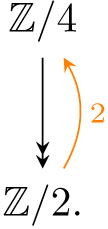
Indeed, the elements $b_L+b_R-2$
and
$b_L+b_R-2$
and $b_R-2$
in
$b_R-2$
in $N_e^{\mathcal{K}}(\mathbb{F}_2)$
are in the image of the transfers from
$N_e^{\mathcal{K}}(\mathbb{F}_2)$
are in the image of the transfers from $D$
and
$D$
and $R$
, respectively. Setting those elements equal to zero produces
$R$
, respectively. Setting those elements equal to zero produces $\mathbb{Z}/4$
as a quotient ring:
$\mathbb{Z}/4$
as a quotient ring:
 \begin{equation*} \frac {\mathbb{Z}/8 \oplus \mathbb{Z}/2\{b_L, b_R\}}{ -2 + b_R, -2 + b_L + b_R} \cong \mathbb{Z}/4. \end{equation*}
2.4.
The norm
$N_{C_2}^{\mathcal{K}}(\underline{{\mathbb{F}}_2})$

We can use Proposition2.7 to compute the norms $n_{H}^{\mathcal{K}}(\underline {{\mathbb{F}}_2})$
for
$n_{H}^{\mathcal{K}}(\underline {{\mathbb{F}}_2})$
for $H \in \{L,D,R\}$
. We will focus on the case
$H \in \{L,D,R\}$
. We will focus on the case $H = D$
; the other cases are similar.
$H = D$
; the other cases are similar.
Proposition 2.15.
The value of the $\mathcal{K}$
-Tambara functor
$\mathcal{K}$
-Tambara functor $n_D^{\mathcal{K}}(\underline {{\mathbb{F}}_2})$
at the trivial orbit
$n_D^{\mathcal{K}}(\underline {{\mathbb{F}}_2})$
at the trivial orbit ${\mathcal{K}}/{\mathcal{K}}$
is the ring
${\mathcal{K}}/{\mathcal{K}}$
is the ring
 \begin{equation*} n_D^{\mathcal{K}}(\underline {{\mathbb{F}}_2})({\mathcal{K}}/{\mathcal{K}}) \cong \displaystyle \mathchoice {{\mathbb{Z}/4[c]}\big /\!{(2c, c^2),}} {{}^{\mathbb{Z}/4[c]}\!/_{\!(2c, c^2),}}{ \mathbb{Z}/4[c] / (2c, c^2),}{ \mathbb{Z}/4[c] / (2c, c^2),} \end{equation*}
where $c$
is the image of
$c$
is the image of $t_R+2$
under the surjection
$t_R+2$
under the surjection $\underline {A} \twoheadrightarrow n_D^{\mathcal{K}}(\underline {{\mathbb{F}}_2})$
.
$\underline {A} \twoheadrightarrow n_D^{\mathcal{K}}(\underline {{\mathbb{F}}_2})$
.
Proof.
Let $\underline {I}$
be the Tambara ideal of
$\underline {I}$
be the Tambara ideal of $\underline {A}$
generated by
$\underline {A}$
generated by $2 \in \underline {A}({\mathcal{K}}/D)$
. By Proposition2.7,
$2 \in \underline {A}({\mathcal{K}}/D)$
. By Proposition2.7, $n_D^{\mathcal{K}}(\underline {{\mathbb{F}}_2})$
is the quotient of
$n_D^{\mathcal{K}}(\underline {{\mathbb{F}}_2})$
is the quotient of $\underline {A}$
by
$\underline {A}$
by $\underline {I}$
. Since
$\underline {I}$
. Since $\textrm {res}^D_e(2) = 2$
, this ideal contains the ideal of
$\textrm {res}^D_e(2) = 2$
, this ideal contains the ideal of $\underline {A}$
generated by
$\underline {A}$
generated by $2 \in \underline {A}({\mathcal{K}}/e)$
. Hence,
$2 \in \underline {A}({\mathcal{K}}/e)$
. Hence, $n_D^{\mathcal{K}}(\underline {{\mathbb{F}}_2})$
is a further quotient of
$n_D^{\mathcal{K}}(\underline {{\mathbb{F}}_2})$
is a further quotient of $n_e^{\mathcal{K}}(\mathbb{F}_2)$
by the Tambara ideal
$n_e^{\mathcal{K}}(\mathbb{F}_2)$
by the Tambara ideal $\underline {J}$
generated by
$\underline {J}$
generated by $2 \in n_e^{\mathcal{K}}(\mathbb{F}_2)({\mathcal{K}}/D)$
.
$2 \in n_e^{\mathcal{K}}(\mathbb{F}_2)({\mathcal{K}}/D)$
.
At the top level $n_e^{\mathcal{K}}(\mathbb{F}_2)({\mathcal{K}}/{\mathcal{K}})$
, the ideal
$n_e^{\mathcal{K}}(\mathbb{F}_2)({\mathcal{K}}/{\mathcal{K}})$
, the ideal $\underline {J}({\mathcal{K}}/{\mathcal{K}})$
is generated by
$\underline {J}({\mathcal{K}}/{\mathcal{K}})$
is generated by $\textrm {nm}_D^{\mathcal{K}}(2)$
and
$\textrm {nm}_D^{\mathcal{K}}(2)$
and ${\textrm {tr}}_D^{\mathcal{K}}(2)$
. The
${\textrm {tr}}_D^{\mathcal{K}}(2)$
. The ${\mathcal{K}}/L$
and
${\mathcal{K}}/L$
and ${\mathcal{K}}/R$
levels do not contribute any generators because
${\mathcal{K}}/R$
levels do not contribute any generators because $\underline {J}({\mathcal{K}}/L) = \underline {J}({\mathcal{K}}/R) = 0$
. By Tambara reciprocity,
$\underline {J}({\mathcal{K}}/L) = \underline {J}({\mathcal{K}}/R) = 0$
. By Tambara reciprocity,
 \begin{align*} \textrm {nm}_D^{\mathcal{K}}(2) = \textrm {nm}_D^{\mathcal{K}}(1+1) &= \textrm {nm}_D^{\mathcal{K}}(1) + \textrm {nm}_D^{\mathcal{K}}(1) + {\textrm {tr}}_D^{\mathcal{K}}(1) \\ &= 1 + 1 + (b_L + b_R -2) \\ &= b_L + b_R \\[5pt] {\textrm {tr}}_D^{\mathcal{K}}(2) &= 2(b_L + b_R - 2) \\ &= 2 b_L + 2b_R - 4 \\ &= -4 \end{align*}
So $n_D^{\mathcal{K}}(\underline {{\mathbb{F}}_2})({\mathcal{K}}/{\mathcal{K}})$
is the quotient of
$n_D^{\mathcal{K}}(\underline {{\mathbb{F}}_2})({\mathcal{K}}/{\mathcal{K}})$
is the quotient of $n_e^{\mathcal{K}}(\mathbb{F}_2)({\mathcal{K}}/{\mathcal{K}})$
by the ideal
$n_e^{\mathcal{K}}(\mathbb{F}_2)({\mathcal{K}}/{\mathcal{K}})$
by the ideal $(b_L + b_R, -4)$
. From Proposition2.10,
$(b_L + b_R, -4)$
. From Proposition2.10,
 \begin{equation*} n_e^{\mathcal{K}}(\mathbb{F}_2)({\mathcal{K}}/{\mathcal{K}}) \cong \displaystyle \mathchoice {{{}^{\mathbb{Z}}\!/_{\!8}[b_L,b_R]}\big /\!{\big(2b_L,2b_R,b_L^2,b_R^2,b_Lb_R\big)}} {{}^{{}^{\mathbb{Z}}\!/_{\!8}[b_L,b_R]}\!/_{\!\big(2b_L,2b_R,b_L^2,b_R^2,b_Lb_R\big)}}{ {}^{\mathbb{Z}}\!/_{\!8}[b_L,b_R] / \big(2b_L,2b_R,b_L^2,b_R^2,b_Lb_R\big)}{ {}^{\mathbb{Z}}\!/_{\!8}[b_L,b_R] / \big(2b_L,2b_R,b_L^2,b_R^2,b_Lb_R\big)} . \end{equation*}
The relation $b_L + b_R$
allows us to identify the two generators, and the
$b_L + b_R$
allows us to identify the two generators, and the $-4$
allows us to replace the
$-4$
allows us to replace the $\mathbb{Z}/8$
by a
$\mathbb{Z}/8$
by a $\mathbb{Z}/4$
. Writing
$\mathbb{Z}/4$
. Writing $c$
for the image of
$c$
for the image of $b_R$
in the quotient, we have
$b_R$
in the quotient, we have
 \begin{equation*} n_D^{\mathcal{K}}(\underline {{\mathbb{F}}_2})({\mathcal{K}}/{\mathcal{K}}) \cong \displaystyle \mathchoice {{{}^{\mathbb{Z}}\!/_{\!4}[c]}\big /\!{(2c,c^2).}} {{}^{{}^{\mathbb{Z}}\!/_{\!4}[c]}\!/_{\!(2c,c^2).}}{ {}^{\mathbb{Z}}\!/_{\!4}[c] / (2c,c^2).}{ {}^{\mathbb{Z}}\!/_{\!4}[c] / (2c,c^2).} \end{equation*}
Remark 2.16.
In the proof of the previous proposition, we simplified the computation of the Tambara functor $n_D^{\mathcal{K}}(\underline {{\mathbb{F}}_2})$
by recognizing it as a quotient of
$n_D^{\mathcal{K}}(\underline {{\mathbb{F}}_2})$
by recognizing it as a quotient of $n_e^{\mathcal{K}}(\underline {{\mathbb{F}}_2})$
. Such a strategy for computing norms of
$n_e^{\mathcal{K}}(\underline {{\mathbb{F}}_2})$
. Such a strategy for computing norms of $\underline {{\mathbb{F}}_2}$
should work for other groups as well. Namely, let
$\underline {{\mathbb{F}}_2}$
should work for other groups as well. Namely, let $G$
be a finite group with a subgroup
$G$
be a finite group with a subgroup $H$
such that the
$H$
such that the $H$
-Tambara functor
$H$
-Tambara functor $\underline {{\mathbb{F}}_2}$
is isomorphic to
$\underline {{\mathbb{F}}_2}$
is isomorphic to $\underline {A}/(2_{H/H})$
, where the
$\underline {A}/(2_{H/H})$
, where the $(2_{H/H})$
is the
$(2_{H/H})$
is the $H$
-Tambara ideal of
$H$
-Tambara ideal of $\underline {A}$
generated by
$\underline {A}$
generated by $2 \in \underline {A}(H/H)$
. Then,
$2 \in \underline {A}(H/H)$
. Then, $n_e^G(\mathbb{F}_2) \cong \underline {A}/(2_{G/e})$
and
$n_e^G(\mathbb{F}_2) \cong \underline {A}/(2_{G/e})$
and $n_H^G(\underline {{\mathbb{F}}_2}) \cong \underline {A}/(2_{G/H})$
. The ideal
$n_H^G(\underline {{\mathbb{F}}_2}) \cong \underline {A}/(2_{G/H})$
. The ideal $(2_{G/H})$
contains the ideal
$(2_{G/H})$
contains the ideal $(2_{G/e})$
because
$(2_{G/e})$
because $\textrm {res}^H_e(2) = 2$
, so we may realize
$\textrm {res}^H_e(2) = 2$
, so we may realize $n_H^G(\underline {{\mathbb{F}}_2})$
as the quotient of
$n_H^G(\underline {{\mathbb{F}}_2})$
as the quotient of $n_e^G(\mathbb{F}_2)$
by the Tambara ideal generated by the element
$n_e^G(\mathbb{F}_2)$
by the Tambara ideal generated by the element $2 \in n_e^G(\mathbb{F}_2)(G/H)$
.
$2 \in n_e^G(\mathbb{F}_2)(G/H)$
.
In particular, when $H$
is a maximal proper subgroup,
$H$
is a maximal proper subgroup, $n_H^G(\underline {{\mathbb{F}}_2})(G/G)$
is the quotient of
$n_H^G(\underline {{\mathbb{F}}_2})(G/G)$
is the quotient of $n_e^G(\mathbb{F}_2)(G/G)$
by the ideal generated by
$n_e^G(\mathbb{F}_2)(G/G)$
by the ideal generated by ${\textrm {tr}}_H^G(2)$
and
${\textrm {tr}}_H^G(2)$
and $\textrm {nm}_H^G(2)$
. When
$\textrm {nm}_H^G(2)$
. When $H$
is not maximal, the generating set is a little more complicated; see [Reference Nakaoka17, Proposition 3.4] for a description of the generators.
$H$
is not maximal, the generating set is a little more complicated; see [Reference Nakaoka17, Proposition 3.4] for a description of the generators.
Together with the facts that $\textrm {res}^{\mathcal{K}}_D n_D^{\mathcal{K}}(\underline {{\mathbb{F}}_2}) = \underline {{\mathbb{F}}_2}$
as in (2.12) and
$\textrm {res}^{\mathcal{K}}_D n_D^{\mathcal{K}}(\underline {{\mathbb{F}}_2}) = \underline {{\mathbb{F}}_2}$
as in (2.12) and $\textrm {res}^{\mathcal{K}}_H n_D^{\mathcal{K}}(\underline {{\mathbb{F}}_2}) \cong n_e^{C_2}(\mathbb{Z}/2)$
via the double coset formula for
$\textrm {res}^{\mathcal{K}}_H n_D^{\mathcal{K}}(\underline {{\mathbb{F}}_2}) \cong n_e^{C_2}(\mathbb{Z}/2)$
via the double coset formula for $H \in \{L,R\}$
, Proposition2.15 allows us to determine the
$H \in \{L,R\}$
, Proposition2.15 allows us to determine the $\mathcal{K}$
-Tambara functor
$\mathcal{K}$
-Tambara functor $n_D^{\mathcal{K}}(\underline {{\mathbb{F}}_2})$
, pictured in Figure 3.
$n_D^{\mathcal{K}}(\underline {{\mathbb{F}}_2})$
, pictured in Figure 3.
The norm $\textrm {nm}_D^{\mathcal{K}}$
is determined by
$\textrm {nm}_D^{\mathcal{K}}$
is determined by $\textrm {nm}_D^{\mathcal{K}}(0) = 0$
and
$\textrm {nm}_D^{\mathcal{K}}(0) = 0$
and $\textrm {nm}_D^{\mathcal{K}}(1) = 1$
. The norms
$\textrm {nm}_D^{\mathcal{K}}(1) = 1$
. The norms $\textrm {nm}_H^{\mathcal{K}}$
for
$\textrm {nm}_H^{\mathcal{K}}$
for $H \in \{L,R\}$
are determined by
$H \in \{L,R\}$
are determined by $\textrm {nm}_H^{\mathcal{K}}(0) = 0$
,
$\textrm {nm}_H^{\mathcal{K}}(0) = 0$
, $\textrm {nm}_H^{\mathcal{K}}(1) = 1$
and Tambara reciprocity (Proposition2.13). In particular,
$\textrm {nm}_H^{\mathcal{K}}(1) = 1$
and Tambara reciprocity (Proposition2.13). In particular, $\textrm {nm}_H^{\mathcal{K}}(2) = c$
and
$\textrm {nm}_H^{\mathcal{K}}(2) = c$
and $\textrm {nm}_H^{\mathcal{K}}(3) = 1+c$
for
$\textrm {nm}_H^{\mathcal{K}}(3) = 1+c$
for $H \in \{L,R\}$
.
$H \in \{L,R\}$
.
The $\mathcal{K}$
-Tambara functor
$\mathcal{K}$
-Tambara functor $n_D^{\mathcal{K}}(\underline {{\mathbb{F}}_2})$
.
$n_D^{\mathcal{K}}(\underline {{\mathbb{F}}_2})$
.

The following result about $n_D^{\mathcal{K}} \underline {{\mathbb{F}}_2}$
-modules will be of use later in the analysis of exact sequences of Mackey functors.
$n_D^{\mathcal{K}} \underline {{\mathbb{F}}_2}$
-modules will be of use later in the analysis of exact sequences of Mackey functors.
Lemma 2.17.
Suppose that $\underline {M}$
is a module over
$\underline {M}$
is a module over $n_D^{\mathcal{K}} \underline {{\mathbb{F}}_2}$
such that
$n_D^{\mathcal{K}} \underline {{\mathbb{F}}_2}$
such that $\underline {M}({\mathcal{K}}/D)=0$
. Then
$\underline {M}({\mathcal{K}}/D)=0$
. Then $\underline {M}({\mathcal{K}}/{\mathcal{K}})$
is 2-torsion.
$\underline {M}({\mathcal{K}}/{\mathcal{K}})$
is 2-torsion.
Proof.
Let $x\in \underline {M}({\mathcal{K}}/{\mathcal{K}})$
. Since
$x\in \underline {M}({\mathcal{K}}/{\mathcal{K}})$
. Since $\underline {M}({\mathcal{K}}/D)$
vanishes, we certainly have that
$\underline {M}({\mathcal{K}}/D)$
vanishes, we certainly have that ${\textrm {tr}}_D^{\mathcal{K}} \textrm {res}^{\mathcal{K}}_D x$
must be zero. On the other hand, Frobenius reciprocity gives
${\textrm {tr}}_D^{\mathcal{K}} \textrm {res}^{\mathcal{K}}_D x$
must be zero. On the other hand, Frobenius reciprocity gives
 \begin{equation*} {\textrm {tr}}_D^{\mathcal{K}} \textrm {res}^{\mathcal{K}}_D(x) = {\textrm {tr}}_D^{\mathcal{K}} \textrm {res}^{\mathcal{K}}_D(1\cdot x) = {\textrm {tr}}_D^{\mathcal{K}}\textrm {res}^{\mathcal{K}}_D(1) \cdot x = 2\cdot x. \end{equation*}
3. Homotopical background
In this section, we collect some facts that will be useful in our computations below.
3.1.
Eilenberg–Mac Lane
$\mathcal{K}$
-spectra

We review here some facts about equivariant Eilenberg–Mac Lane spectra for the group $\mathcal{K}$
. Similar statements hold more generally for any finite group.
$\mathcal{K}$
. Similar statements hold more generally for any finite group.
The Eilenberg–Mac Lane spectrum of a $\mathcal{K}$
-Mackey
$\mathcal{K}$
-Mackey $\underline {M}$
functor is the
$\underline {M}$
functor is the $\mathcal{K}$
-spectrum
$\mathcal{K}$
-spectrum $\boldsymbol{\mathscr{H}} \underline {M}$
whose homotopy Mackey functors are determined by
$\boldsymbol{\mathscr{H}} \underline {M}$
whose homotopy Mackey functors are determined by
 \begin{equation*} \underline {\pi }_n \boldsymbol{\mathscr{H}} \underline {M} = \begin{cases} \underline {M} & n = 0\\ 0 & n \neq 0. \end{cases} \end{equation*}
Although the only nonzero integer-graded homotopy group of $\boldsymbol{\mathscr{H}} \underline {M}$
is
$\boldsymbol{\mathscr{H}} \underline {M}$
is $\underline {\pi }_0$
, suspensions of
$\underline {\pi }_0$
, suspensions of $\boldsymbol{\mathscr{H}}\underline {M}$
by representation spheres may have more complicated homotopy. See, for example, Figure 6 in the
$\boldsymbol{\mathscr{H}}\underline {M}$
by representation spheres may have more complicated homotopy. See, for example, Figure 6 in the $C_2$
-equivariant case. An important property of the functor
$C_2$
-equivariant case. An important property of the functor $\boldsymbol{\mathscr{H}} \colon {\mathscr{M}\text{ack}}({\mathcal{K}}) \to \mathscr{S}\text{p}^{\mathcal{K}}$
is that it sends short exact sequences of
$\boldsymbol{\mathscr{H}} \colon {\mathscr{M}\text{ack}}({\mathcal{K}}) \to \mathscr{S}\text{p}^{\mathcal{K}}$
is that it sends short exact sequences of $\mathcal{K}$
-Mackey functors to cofibre sequences of
$\mathcal{K}$
-Mackey functors to cofibre sequences of $\mathcal{K}$
-spectra.
$\mathcal{K}$
-spectra.
The Eilenberg–Mac Lane spectrum functor also commutes with several change of group functors. For $H$
a subgroup of
$H$
a subgroup of $\mathcal{K}$
, let
$\mathcal{K}$
, let $\uparrow _H^{\mathcal{K}}$
and
$\uparrow _H^{\mathcal{K}}$
and $\downarrow ^{\mathcal{K}}_H$
denote the induction and restriction functors, respectively, either between
$\downarrow ^{\mathcal{K}}_H$
denote the induction and restriction functors, respectively, either between $\mathcal{K}$
- and
$\mathcal{K}$
- and $H$
-Mackey functors or between
$H$
-Mackey functors or between $\mathcal{K}$
- and
$\mathcal{K}$
- and $H$
-spectra.
$H$
-spectra.
Proposition 3.1.
Let $\underline {M}$
be a
$\underline {M}$
be a $\mathcal{K}$
-Mackey functor and
$\mathcal{K}$
-Mackey functor and $\underline {N}$
an
$\underline {N}$
an $H$
-Mackey functor. Then,
$H$
-Mackey functor. Then,
-
(a)
$\downarrow _H^{\mathcal{K}}\! \boldsymbol{\mathscr{H}}(\underline {M}) \simeq \mathbf{H}\left (\!\downarrow _H^{\mathcal{K}}\!\underline {M}\right )$
-
(b)
$\uparrow _H^{\mathcal{K}}\! \mathbf{H}(\underline {N}) \simeq \boldsymbol{\mathscr{H}}\left (\uparrow _H^{\mathcal{K}}\!\underline {N}\right )$
.


We include a proof of this well-known result as we were not able to find a reference in the literature.
Proof. Consider the diagram of adjunctions
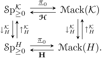
We claim that the diagram of left adjoints commutes. Namely, we claim that for every (connective) $\mathcal{K}$
-spectrum
$\mathcal{K}$
-spectrum $X$
, we have a natural isomorphism of
$X$
, we have a natural isomorphism of $H$
-Mackey functors
$H$
-Mackey functors $\underline {\pi }_0 \! \downarrow ^{\mathcal{K}}_H \! X \cong \, \downarrow ^{\mathcal{K}}_H \! \underline {\pi }_0 X$
. Indeed, we have isomorphisms, natural in
$\underline {\pi }_0 \! \downarrow ^{\mathcal{K}}_H \! X \cong \, \downarrow ^{\mathcal{K}}_H \! \underline {\pi }_0 X$
. Indeed, we have isomorphisms, natural in $H$
-sets
$H$
-sets $T$
,
$T$
,
 \begin{align*} \underline {\pi }_0 (\!\downarrow ^{\mathcal{K}}_H \! X) (T) \cong [ T_+, \downarrow ^{\mathcal{K}}_H \! X]^H \cong [ ({\mathcal{K}}\times _H T)_+, X]^{\mathcal{K}} \cong \, \downarrow ^{\mathcal{K}}_H \! (\underline {\pi }_0 X) (T). \end{align*}
It follows that the diagram of right adjoints commutes, which is item (b).
On the other hand, both vertical adjunctions are ambidextrous. Thus, the isomorphism (a) would follow from an isomorphism of $\mathcal{K}$
-Mackey functors
$\mathcal{K}$
-Mackey functors $\underline {\pi }_0 \! \uparrow ^{\mathcal{K}}_H \! Y \cong \, \uparrow ^{\mathcal{K}}_H \! \underline {\pi }_0 Y$
, natural in
$\underline {\pi }_0 \! \uparrow ^{\mathcal{K}}_H \! Y \cong \, \uparrow ^{\mathcal{K}}_H \! \underline {\pi }_0 Y$
, natural in $H$
-spectra
$H$
-spectra $Y$
. This is provided by the isomorphism, natural in
$Y$
. This is provided by the isomorphism, natural in $\mathcal{K}$
-sets
$\mathcal{K}$
-sets $W$
,
$W$
,
 \begin{equation*} \underline {\pi }_0 (\!\uparrow ^{\mathcal{K}}_H \! Y) (W) = [W_+, \uparrow _H^{\mathcal{K}} Y]^{\mathcal{K}} \cong [\!\downarrow ^{\mathcal{K}}_H W_+, Y]^H \cong \ \uparrow _H^{\mathcal{K}} \!(\underline {\pi }_0 Y) (W). \end{equation*}
Since the diagram of left adjoints commutes, so does the diagram of right adjoints. This establishes (a).
However, taking the Eilenberg–Mac Lane spectrum does not commute with norms. For example, $N_e^{C_2}H\mathbb{F}_2$
is not Eilenberg–Mac Lane, as its underlying spectrum is
$N_e^{C_2}H\mathbb{F}_2$
is not Eilenberg–Mac Lane, as its underlying spectrum is $H\mathbb{F}_2\wedge H\mathbb{F}_2$
, whose homotopy groups are the dual Steenrod algebra. On the other hand, for
$H\mathbb{F}_2\wedge H\mathbb{F}_2$
, whose homotopy groups are the dual Steenrod algebra. On the other hand, for $X$
a connective
$X$
a connective $H$
-spectrum, there is an isomorphism
$H$
-spectrum, there is an isomorphism $\underline {\pi }_0 N_H^{\mathcal{K}} X \cong N_H^{\mathcal{K}} \underline {\pi }_0 X$
[Reference Ullman21, Corollary 3.2].
$\underline {\pi }_0 N_H^{\mathcal{K}} X \cong N_H^{\mathcal{K}} \underline {\pi }_0 X$
[Reference Ullman21, Corollary 3.2].
3.2.
${\textrm {RO}}({\mathcal{K}})$
-graded suspensions

The abelian group ${\textrm {RO}}({\mathcal{K}})$
is a free abelian group of rank 4 generated by the trivial representation
${\textrm {RO}}({\mathcal{K}})$
is a free abelian group of rank 4 generated by the trivial representation $1$
and three one-dimensional representations
$1$
and three one-dimensional representations $\sigma _L$
,
$\sigma _L$
, $\sigma _D$
and
$\sigma _D$
and $\sigma _R$
. For a subgroup
$\sigma _R$
. For a subgroup $H \in \{L,D,R\}$
of
$H \in \{L,D,R\}$
of $\mathcal{K}$
, the representation
$\mathcal{K}$
, the representation $\sigma _H$
corresponds to the sign representation
$\sigma _H$
corresponds to the sign representation $\sigma$
of
$\sigma$
of ${\mathcal{K}}/H\cong C_2$
, where
${\mathcal{K}}/H\cong C_2$
, where $\mathcal{K}$
acts via the quotient homomorphism
$\mathcal{K}$
acts via the quotient homomorphism ${\mathcal{K}} \to {\mathcal{K}}/H$
. We also write
${\mathcal{K}} \to {\mathcal{K}}/H$
. We also write $\rho = 1 + \sigma _L + \sigma _D + \sigma _R$
for the regular representation of
$\rho = 1 + \sigma _L + \sigma _D + \sigma _R$
for the regular representation of $\mathcal{K}$
and
$\mathcal{K}$
and $\overline {\rho } = \rho - 1$
for the reduced regular representation.
$\overline {\rho } = \rho - 1$
for the reduced regular representation.
Because we are interested in the ${\textrm {RO}}({\mathcal{K}})$
-graded homotopy of
${\textrm {RO}}({\mathcal{K}})$
-graded homotopy of $\mathcal{K}$
-spectra, we will frequently suspend by (virtual) representation spheres
$\mathcal{K}$
-spectra, we will frequently suspend by (virtual) representation spheres $S^V$
for
$S^V$
for $V \in {\textrm {RO}}({\mathcal{K}})$
. We are primarily interested in
$V \in {\textrm {RO}}({\mathcal{K}})$
. We are primarily interested in $\overline {\rho }$
-suspensions of
$\overline {\rho }$
-suspensions of $\mathcal{K}$
-spectra, but we will also find occasion to use
$\mathcal{K}$
-spectra, but we will also find occasion to use $\sigma _H$
-suspensions. The suspension
$\sigma _H$
-suspensions. The suspension $\Sigma ^{\sigma _H}$
fits into a cofibre sequence
$\Sigma ^{\sigma _H}$
fits into a cofibre sequence
 \begin{equation*} {\mathcal{K}}/H_+ \wedge X \to X \to \Sigma ^{\sigma _H} X. \end{equation*}
The fibre has an alternative description, by the shearing isomorphism:
Proposition 3.2 (Shearing). Let $X$
be a
$X$
be a $\mathcal{K}$
-spectrum and let
$\mathcal{K}$
-spectrum and let $H$
be a subgroup of
$H$
be a subgroup of $\mathcal{K}$
. Then,
$\mathcal{K}$
. Then,
 \begin{equation*} {\mathcal{K}}/H_+ \wedge X \simeq \, \uparrow ^{\mathcal{K}}_H\downarrow ^{\mathcal{K}}_H\! X, \end{equation*}
where $\downarrow ^{\mathcal{K}}_H$
denotes the restriction from
$\downarrow ^{\mathcal{K}}_H$
denotes the restriction from $\mathcal{K}$
-spectra to
$\mathcal{K}$
-spectra to $H$
-spectra and
$H$
-spectra and $\uparrow _H^{\mathcal{K}}$
the induction.
$\uparrow _H^{\mathcal{K}}$
the induction.
In particular, when $X$
is an Eilenberg–Mac Lane spectrum, we have
$X$
is an Eilenberg–Mac Lane spectrum, we have
 \begin{equation*} {\mathcal{K}}/H_+ \wedge \boldsymbol{\mathscr{H}} \underline {M} \simeq \uparrow ^{\mathcal{K}}_H\downarrow ^{\mathcal{K}}_H \boldsymbol{\mathscr{H}} \underline {M} \simeq \boldsymbol{\mathscr{H}}\left (\uparrow ^{\mathcal{K}}_H\downarrow ^{\mathcal{K}}_H\!\underline {M}\right ). \end{equation*}
A useful consequence of this is the following:
Corollary 3.3.
Let $X$
be a
$X$
be a $\mathcal{K}$
-spectrum and let
$\mathcal{K}$
-spectrum and let $H \in \{L,D,R\}$
. If the restriction of
$H \in \{L,D,R\}$
. If the restriction of $X$
to
$X$
to $H$
is contractible, then
$H$
is contractible, then
 \begin{equation*} \Sigma ^{\sigma _H} X \simeq X. \end{equation*}
3.3. Inflation functors
Our main computations are $\mathcal{K}$
-equivariant. However, we often make comparisons to
$\mathcal{K}$
-equivariant. However, we often make comparisons to $C_2$
-equivariant computations, as
$C_2$
-equivariant computations, as $C_2$
appears both as a subgroup and a quotient of
$C_2$
appears both as a subgroup and a quotient of $\mathcal{K}$
. For reference, we display in Figures 6 and 7 the
$\mathcal{K}$
. For reference, we display in Figures 6 and 7 the $RO(C_2)$
-graded homotopy Mackey functors of
$RO(C_2)$
-graded homotopy Mackey functors of $\mathbf{H} \underline {{\mathbb{F}}_2}$
and
$\mathbf{H} \underline {{\mathbb{F}}_2}$
and $\mathbf{H} N_e^{C_2}\mathbb{F}_2$
, respectively. The Mackey functors appearing in those charts are as shown in Table 3.
$\mathbf{H} N_e^{C_2}\mathbb{F}_2$
, respectively. The Mackey functors appearing in those charts are as shown in Table 3.
We follow [Reference Hill8, Section 4] in writing $\phi ^*_H \underline {M}$
for the inflation along the quotient
$\phi ^*_H \underline {M}$
for the inflation along the quotient ${\mathcal{K}} \to {\mathcal{K}}/H$
of the
${\mathcal{K}} \to {\mathcal{K}}/H$
of the ${\mathcal{K}}/H$
-Mackey functor
${\mathcal{K}}/H$
-Mackey functor $\underline {M}$
, for any subgroup
$\underline {M}$
, for any subgroup $H \leq {\mathcal{K}}$
. Since the groups
$H \leq {\mathcal{K}}$
. Since the groups ${\mathcal{K}}/H$
are canonically isomorphic for all
${\mathcal{K}}/H$
are canonically isomorphic for all $H$
in
$H$
in $\{L,D,R\}$
, we write
$\{L,D,R\}$
, we write $\phi ^*_{LDR}\underline {M}$
as shorthand for the sum
$\phi ^*_{LDR}\underline {M}$
as shorthand for the sum $\phi ^*_L \underline {M} \oplus \phi ^*_D \underline {M} \oplus \phi ^*_R \underline {M}$
for any
$\phi ^*_L \underline {M} \oplus \phi ^*_D \underline {M} \oplus \phi ^*_R \underline {M}$
for any $C_2$
-Mackey functor
$C_2$
-Mackey functor $\underline {M}$
. See Table 2. As in [Reference Guillou and Yarnall5], we write
$\underline {M}$
. See Table 2. As in [Reference Guillou and Yarnall5], we write $\underline {g}$
for the fully inflated Mackey functor
$\underline {g}$
for the fully inflated Mackey functor $\phi ^*_{{\mathcal{K}}}\mathbb{F}$
(see Table 4).
$\phi ^*_{{\mathcal{K}}}\mathbb{F}$
(see Table 4).
The inflation functor $\phi _H^* \colon {\mathscr{M}\text{ack}}(C_2) \to {\mathscr{M}\text{ack}}({\mathcal{K}})$
, where we identify
$\phi _H^* \colon {\mathscr{M}\text{ack}}(C_2) \to {\mathscr{M}\text{ack}}({\mathcal{K}})$
, where we identify $C_2 \cong {\mathcal{K}}/H$
. We also write
$C_2 \cong {\mathcal{K}}/H$
. We also write $\phi ^*_{LDR} \underline {M} \;:\!=\; \phi _L^* \underline {M} \oplus \phi _D^* \underline {M} \oplus \phi _R^* \underline {M}$

The inflation functor $\phi _H^*$
in fact extends to a ‘geometric inflation’ functor on spectra and
$\phi _H^*$
in fact extends to a ‘geometric inflation’ functor on spectra and $\phi _H^* \mathbf{H} \underline {M} \simeq \boldsymbol{\mathscr{H}} \phi _H^* \underline {M}$
. In fact, by considering the Postnikov tower for any
$\phi _H^* \mathbf{H} \underline {M} \simeq \boldsymbol{\mathscr{H}} \phi _H^* \underline {M}$
. In fact, by considering the Postnikov tower for any ${\mathcal{K}}/H$
-spectrum
${\mathcal{K}}/H$
-spectrum $X$
, one gets more generally an isomorphism of
$X$
, one gets more generally an isomorphism of $\mathcal{K}$
-Mackey functors
$\mathcal{K}$
-Mackey functors
 \begin{equation} \underline {\pi }_n \phi _H^* X \cong \phi _H^* \underline {\pi }_n X. \end{equation}
We will use this frequently. More importantly, for any $\mathcal{K}$
-representation
$\mathcal{K}$
-representation $V$
, we have [Reference Hill8, Corollary 4.6]
$V$
, we have [Reference Hill8, Corollary 4.6]
 \begin{equation} \Sigma ^V \boldsymbol{\mathscr{H}} \phi _H^* \underline {M} \simeq \phi _H^* \big(\Sigma ^{V^H} {\mathbf{H}} \underline {M}\big) \end{equation}
where $V^H$
is considered as a representation of
$V^H$
is considered as a representation of ${\mathcal{K}}/H$
.
${\mathcal{K}}/H$
.
This, combined with Figure 6, gives the following useful equivalences:
Proposition 3.6. We have equivalences
-
(a)
$\Sigma ^{\overline {\rho }} \boldsymbol{\mathscr{H}} \underline {g} \simeq \boldsymbol{\mathscr{H}} \underline {g}$
-
(b)
$\Sigma ^{\overline {\rho }} \boldsymbol{\mathscr{H}} \phi _H^* \underline {{\mathbb{F}}_2}^* \simeq \Sigma ^1 \boldsymbol{\mathscr{H}} \phi _H^*\, \underline {f}\ $
for
$H\in \{L,D,R\}$
-
(c)
$\Sigma ^{\overline {\rho }} \boldsymbol{\mathscr{H}} \phi _H^*\, \underline {f} \simeq \Sigma ^1 \boldsymbol{\mathscr{H}} \phi _H^*\, \underline {{\mathbb{F}}_2}\ $
for
$H\in \{L,D,R\}$
.





where $\underline {f}$
is as displayed in Table
3
.
$\underline {f}$
is as displayed in Table
3
.
4. The homotopy of
$\boldsymbol{\mathscr{H}} N_e^{\mathcal{K}} \mathbb{F}_2$

In this section, we compute the homotopy Mackey functors $\underline {\pi }_{\blacklozenge } \boldsymbol{\mathscr{HN}}$
, where
$\underline {\pi }_{\blacklozenge } \boldsymbol{\mathscr{HN}}$
, where $\boldsymbol{\mathscr{N}}$
will often be used as an abbreviation for
$\boldsymbol{\mathscr{N}}$
will often be used as an abbreviation for $ N_e^{\mathcal{K}} \mathbb{F}_2$
. The results are displayed in Figure 11.
$ N_e^{\mathcal{K}} \mathbb{F}_2$
. The results are displayed in Figure 11.
Remark 4.1.
For $k\geq 0$
, the homology groups
$k\geq 0$
, the homology groups $\underline {H}_n(S^{k\overline {\rho }};\;\;\boldsymbol{\mathscr{N}}) \cong \underline {\pi }_{n-k\overline {\rho }}\boldsymbol{\mathscr{HN}}$
are concentrated in degrees
$\underline {H}_n(S^{k\overline {\rho }};\;\;\boldsymbol{\mathscr{N}}) \cong \underline {\pi }_{n-k\overline {\rho }}\boldsymbol{\mathscr{HN}}$
are concentrated in degrees $n\geq 0$
. We will refer to this portion of
$n\geq 0$
. We will refer to this portion of $\underline {\pi }_{\blacklozenge } \boldsymbol{\mathscr{HN}}$
as the
positive cone
. It appears in the fourth quadrant of Figure
11
. Similarly, the cohomology groups
$\underline {\pi }_{\blacklozenge } \boldsymbol{\mathscr{HN}}$
as the
positive cone
. It appears in the fourth quadrant of Figure
11
. Similarly, the cohomology groups $\underline {H}^n(S^{k\overline {\rho }};\;\boldsymbol{\mathscr{N}}) \cong \pi _{-n+k\overline {\rho }} \boldsymbol{\mathscr{HN}}$
are concentrated in degrees
$\underline {H}^n(S^{k\overline {\rho }};\;\boldsymbol{\mathscr{N}}) \cong \pi _{-n+k\overline {\rho }} \boldsymbol{\mathscr{HN}}$
are concentrated in degrees $n\geq 0$
. We will refer to this portion as the
negative cone
. It appears in the second quadrant of Figure
11
.
$n\geq 0$
. We will refer to this portion as the
negative cone
. It appears in the second quadrant of Figure
11
.
We proceed with a computation of the positive cone for $\boldsymbol{\mathscr{HN}}$
followed by that of the negative cone.
$\boldsymbol{\mathscr{HN}}$
followed by that of the negative cone.
4.1.
The positive cone of
$\boldsymbol{\mathscr{H}} N_e^{{\mathcal{K}}} \mathbb{F}_2$

Here we compute the homotopy Mackey functors of the $\mathcal{K}$
-spectra
$\mathcal{K}$
-spectra $\Sigma ^{k\overline {\rho }} \boldsymbol{\mathscr{HN}}$
for
$\Sigma ^{k\overline {\rho }} \boldsymbol{\mathscr{HN}}$
for $k\geq 0$
.
$k\geq 0$
.
We start with the case $k=1$
. Our analysis will rely on cofibre sequences of equivariant Eilenberg–Mac Lane spectra arising from short exact sequences of Mackey functors. In particular, the following Mackey functor
$k=1$
. Our analysis will rely on cofibre sequences of equivariant Eilenberg–Mac Lane spectra arising from short exact sequences of Mackey functors. In particular, the following Mackey functor $\underline {E}$
will be of use.
$\underline {E}$
will be of use.
Definition 4.2.
Let $\underline {E}$
be the cokernel of
$\underline {E}$
be the cokernel of $\underline {{\mathbb{F}}_2}^* \hookrightarrow N_e^{{\mathcal{K}}} \mathbb{F}_2$
. This Mackey functor is displayed below.
$\underline {{\mathbb{F}}_2}^* \hookrightarrow N_e^{{\mathcal{K}}} \mathbb{F}_2$
. This Mackey functor is displayed below.
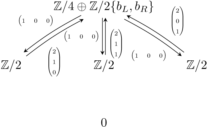
The Mackey functor $\underline {E}$
also fits into a short exact sequence
$\underline {E}$
also fits into a short exact sequence
 \begin{equation} \phi ^*_{LDR} (\underline {{\mathbb{F}}_2}^*) \hookrightarrow \underline {E} \twoheadrightarrow \underline {g}. \end{equation}
Lemma 4.4.
The nonzero homotopy Mackey functors of $\Sigma ^{\overline {\rho }}\boldsymbol{\mathscr{H}}\underline {E}$
are
$\Sigma ^{\overline {\rho }}\boldsymbol{\mathscr{H}}\underline {E}$
are
 \begin{equation*} \underline {\pi }_n \Sigma ^{\overline {\rho }} \boldsymbol{\mathscr{H}} \underline {E} = \begin{cases} \underline {g} & n = 0\\ \phi ^*_{LDR}\, \underline {f} & n = 1 \end{cases} \end{equation*}
Proof.
Applying the functors $\Sigma ^{\overline {\rho }}$
and
$\Sigma ^{\overline {\rho }}$
and $\boldsymbol{\mathscr{H}}$
to the short exact sequence (4.3) yields a cofibre sequence:
$\boldsymbol{\mathscr{H}}$
to the short exact sequence (4.3) yields a cofibre sequence:
 \begin{equation*} \Sigma ^{\overline {\rho }} \boldsymbol{\mathscr{H}} \phi _{LDR}^* \underline {{\mathbb{F}}_2}^* \to \Sigma ^{\overline {\rho }} \boldsymbol{\mathscr{H}} \underline {E} \to \Sigma ^{\overline {\rho }} \boldsymbol{\mathscr{H}} \underline {g}. \end{equation*}
But Proposition3.6 provides equivalences $\Sigma ^{\overline {\rho }} \boldsymbol{\mathscr{H}} \phi _{LDR}^* \underline {{\mathbb{F}}_2}^* \simeq \Sigma ^1 \boldsymbol{\mathscr{H}} \phi _{LDR}^*\, \underline {f}$
and
$\Sigma ^{\overline {\rho }} \boldsymbol{\mathscr{H}} \phi _{LDR}^* \underline {{\mathbb{F}}_2}^* \simeq \Sigma ^1 \boldsymbol{\mathscr{H}} \phi _{LDR}^*\, \underline {f}$
and $\Sigma ^{\overline {\rho }} \boldsymbol{\mathscr{H}} \underline {g} \simeq \boldsymbol{\mathscr{H}} \underline {g}$
, so the homotopy of
$\Sigma ^{\overline {\rho }} \boldsymbol{\mathscr{H}} \underline {g} \simeq \boldsymbol{\mathscr{H}} \underline {g}$
, so the homotopy of $\Sigma ^{\overline {\rho }} \boldsymbol{\mathscr{H}} \underline {E}$
can be read off from the associated long exact sequence.
$\Sigma ^{\overline {\rho }} \boldsymbol{\mathscr{H}} \underline {E}$
can be read off from the associated long exact sequence.
Proposition 4.5.
The nonzero homotopy Mackey functors of $\Sigma ^{\overline {\rho }} \boldsymbol{\mathscr{H}} N_e^{{\mathcal{K}}} \mathbb{F}_2$
are
$\Sigma ^{\overline {\rho }} \boldsymbol{\mathscr{H}} N_e^{{\mathcal{K}}} \mathbb{F}_2$
are
 \begin{equation*} \underline {\pi }_n \Sigma ^{\overline {\rho }} \boldsymbol{\mathscr{H}} N_e^{{\mathcal{K}}} \mathbb{F}_2 \cong \begin{cases} \underline {\mathbb{F}}_2 & n=3 \\ \phi _{LDR}^*\, \underline {f} & n=1 \\ \underline {g} & n=0. \end{cases} \end{equation*}
Proof.
By applying the functors $\Sigma ^{\overline {\rho }}$
and
$\Sigma ^{\overline {\rho }}$
and $\boldsymbol{\mathscr{H}}$
to the defining short exact sequence for
$\boldsymbol{\mathscr{H}}$
to the defining short exact sequence for $\underline {E}$
, we have a cofibre sequence
$\underline {E}$
, we have a cofibre sequence
 \begin{equation*} \Sigma ^{\overline {\rho }}\boldsymbol{\mathscr{H}} \underline {{\mathbb{F}}_2}^* \to \Sigma ^{\overline {\rho }}\boldsymbol{\mathscr{HN}} \to \Sigma ^{\overline {\rho }}\boldsymbol{\mathscr{H}} \underline {E}. \end{equation*}
We understand the homotopy of the fibre: $\Sigma ^{\overline {\rho }} \boldsymbol{\mathscr{H}} \underline {{\mathbb{F}}_2}^*$
is
$\Sigma ^{\overline {\rho }} \boldsymbol{\mathscr{H}} \underline {{\mathbb{F}}_2}^*$
is $\Sigma ^3 \boldsymbol{\mathscr{H}} \underline {{\mathbb{F}}_2}$
by [Reference Guillou and Yarnall5, Proposition 4.2]. We also understand the homotopy of the cofibre by Lemma4.4. The desired homotopy may then be read off from the associated long exact sequence.
$\Sigma ^3 \boldsymbol{\mathscr{H}} \underline {{\mathbb{F}}_2}$
by [Reference Guillou and Yarnall5, Proposition 4.2]. We also understand the homotopy of the cofibre by Lemma4.4. The desired homotopy may then be read off from the associated long exact sequence.
The computation of the homotopy of $\Sigma ^{\overline {\rho }} \boldsymbol{\mathscr{HN}}$
gives a fibre sequence
$\Sigma ^{\overline {\rho }} \boldsymbol{\mathscr{HN}}$
gives a fibre sequence
 \begin{equation} \Sigma ^3 \boldsymbol{\mathscr{H}} \underline {{\mathbb{F}}_2} \to \Sigma ^{\overline {\rho }} \boldsymbol{\mathscr{HN}} \to \Sigma ^{\overline {\rho }} \boldsymbol{\mathscr{H}} \underline {E}. \end{equation}
It turns out that the $(k-1)\overline {\rho }$
-suspension of the map
$(k-1)\overline {\rho }$
-suspension of the map $\Sigma ^3 \boldsymbol{\mathscr{H}} \underline {{\mathbb{F}}_2} \to \Sigma ^{\overline {\rho }} \boldsymbol{\mathscr{HN}}$
detects much of the homotopy of
$\Sigma ^3 \boldsymbol{\mathscr{H}} \underline {{\mathbb{F}}_2} \to \Sigma ^{\overline {\rho }} \boldsymbol{\mathscr{HN}}$
detects much of the homotopy of $\Sigma ^{k\overline {\rho }} \boldsymbol{\mathscr{HN}}$
, as follows from analysis of the suspensions of the cofibre.
$\Sigma ^{k\overline {\rho }} \boldsymbol{\mathscr{HN}}$
, as follows from analysis of the suspensions of the cofibre.
Proposition 4.7.
For $k\geq 2$
, the nonzero homotopy Mackey functors of
$k\geq 2$
, the nonzero homotopy Mackey functors of $\Sigma ^{k\overline {\rho }} \boldsymbol{\mathscr{H}} \underline {E}$
are
$\Sigma ^{k\overline {\rho }} \boldsymbol{\mathscr{H}} \underline {E}$
are
 \begin{equation*} \underline {\pi }_n \Sigma ^{k\overline {\rho }} \boldsymbol{\mathscr{H}} \underline {E} \cong \begin{cases} \phi _{LDR}^* \underline {{\mathbb{F}}_2} & n=k \\ \underline {g}^3 & n \in [2,k-1] \\ \underline {g} & n=0. \end{cases} \end{equation*}
Proof. As in Lemma4.4, we have a fibre sequence
 \begin{equation*} \Sigma ^1 \boldsymbol{\mathscr{H}} \phi _{LDR}^*\, \underline {f} \to \Sigma ^{\overline {\rho }} \boldsymbol{\mathscr{H}} \underline {E} \to \boldsymbol{\mathscr{H}} \underline {g}. \end{equation*}
Suspending this $(k-1)\overline {\rho }$
times yields another fibre sequence
$(k-1)\overline {\rho }$
times yields another fibre sequence
 \begin{equation*} \Sigma ^{1 + (k-1)\overline {\rho }}\boldsymbol{\mathscr{H}} \phi _{LDR}^*\, \underline {f} \to \Sigma ^{k\overline {\rho }} \boldsymbol{\mathscr{H}} \underline {E} \to \Sigma ^{(k-1)\overline {\rho }}\boldsymbol{\mathscr{H}} \underline {g}. \end{equation*}
Applying the equivalences
 \begin{equation*} \Sigma ^{\overline {\rho }} \boldsymbol{\mathscr{H}} \underline {g} \simeq \boldsymbol{\mathscr{H}} \underline {g} \quad \text{and} \quad \Sigma ^{\overline {\rho }} \boldsymbol{\mathscr{H}} \phi _{LDR}^*\, \underline {f} \simeq \Sigma ^1 \boldsymbol{\mathscr{H}} \phi _{LDR}^* \underline {{\mathbb{F}}_2} \end{equation*}
from Proposition3.6, we see that this fibre sequence is equivalent to
 \begin{equation} \Sigma ^{2 + (k-2)\overline {\rho }}\boldsymbol{\mathscr{H}} \phi _{LDR}^*\underline {{\mathbb{F}}_2} \to \Sigma ^{k\overline {\rho }} \boldsymbol{\mathscr{H}} \underline {E} \to \boldsymbol{\mathscr{H}} \underline {g}. \end{equation}
Then by (3.5), the left term becomes
 \begin{equation*} \Sigma ^{2 + (k-2)\overline {\rho }}\boldsymbol{\mathscr{H}} \phi _{LDR}^*\underline {{\mathbb{F}}_2} \simeq \bigvee _{H \in \{L,D,R\}} \phi _{H}^* \left (\Sigma ^{(2 + (k-2){\sigma })} \mathbf{H} \underline {{\mathbb{F}}_2} \right ) \end{equation*}
Here we have used the identification $\overline {\rho }^H \cong \overline {\rho }=\sigma$
for
$\overline {\rho }^H \cong \overline {\rho }=\sigma$
for $H\in \{L,D,R\}$
. We may compute the homotopy of the above using (3.4) and the computation of the
$H\in \{L,D,R\}$
. We may compute the homotopy of the above using (3.4) and the computation of the $C_2$
-Mackey functors
$C_2$
-Mackey functors $\underline {\pi }_\blacklozenge ^{C_2} \mathbf{H} \underline {{\mathbb{F}}_2}$
, as in Figure 6. The result then follows from the long exact sequence associated to (4.8).
$\underline {\pi }_\blacklozenge ^{C_2} \mathbf{H} \underline {{\mathbb{F}}_2}$
, as in Figure 6. The result then follows from the long exact sequence associated to (4.8).
In the case $k=2$
, the cofibre sequence (4.6) and Proposition4.7 give the following computation of
$k=2$
, the cofibre sequence (4.6) and Proposition4.7 give the following computation of $\Sigma ^{2\overline {\rho }} \boldsymbol{\mathscr{HN}}$
.
$\Sigma ^{2\overline {\rho }} \boldsymbol{\mathscr{HN}}$
.
Corollary 4.9.
The nontrivial homotopy Mackey functors of $\Sigma ^{2\overline {\rho }} \boldsymbol{\mathscr{H}} N_e^{\mathcal{K}} \mathbb{F}_2$
are
$\Sigma ^{2\overline {\rho }} \boldsymbol{\mathscr{H}} N_e^{\mathcal{K}} \mathbb{F}_2$
are
 \begin{equation*} \underline {\pi }_n \Sigma ^{2\overline {\rho }} \boldsymbol{\mathscr{H}} N_e^K \mathbb{F}_2 \cong \begin{cases} \underline {\pi }_{n-3} \Sigma ^{\overline {\rho }} \boldsymbol{\mathscr{H}} \underline {\mathbb{F}}_2 & n \geq 3 \\ \phi _{LDR}^* \underline {\mathbb{F}}_2 & n=2 \\ \underline {g} & n=0. \end{cases} \end{equation*}
More generally, combining (4.6) with Proposition4.7 gives the following.
Corollary 4.10.
For $k \geq 2$
, we have isomorphisms
$k \geq 2$
, we have isomorphisms
 \begin{equation*} \underline {\pi }_n \Sigma ^{k\overline {\rho }} \boldsymbol{\mathscr{H}} N_e^{\mathcal{K}} \mathbb{F}_2 \cong \underline {\pi }_n \Sigma ^{3+(k-1)\overline {\rho }} \boldsymbol{\mathscr{H}} \underline {{\mathbb{F}}_2} = \underline {\pi }_{n-3} \Sigma ^{(k-1)\overline {\rho }} \boldsymbol{\mathscr{H}} \underline {{\mathbb{F}}_2} \end{equation*}
for $n \geq k+1$
.
$n \geq k+1$
.
However, starting with $k=3$
, the homotopy of the left and right terms in the sequence
$k=3$
, the homotopy of the left and right terms in the sequence
 \begin{equation} \Sigma ^{3+(k-1)\overline {\rho }} \boldsymbol{\mathscr{H}} \underline {{\mathbb{F}}_2} \to \Sigma ^{k\overline {\rho }} \boldsymbol{\mathscr{HN}} \to \Sigma ^{k\overline {\rho }} \boldsymbol{\mathscr{H}} \underline {E} \end{equation}
begin to overlap. In order to find the lower homotopy Mackey functors of $\Sigma ^{k\overline {\rho }} \boldsymbol{\mathscr{HN}}$
, it is convenient to consider a different sequence. The kernel of the surjection
$\Sigma ^{k\overline {\rho }} \boldsymbol{\mathscr{HN}}$
, it is convenient to consider a different sequence. The kernel of the surjection $\boldsymbol{\mathscr{N}} \twoheadrightarrow \underline {\mathbb{F}}_2$
is
$\boldsymbol{\mathscr{N}} \twoheadrightarrow \underline {\mathbb{F}}_2$
is $\underline {B}(2,0) \oplus \underline {g}^2$
, and we now describe its homotopy.
$\underline {B}(2,0) \oplus \underline {g}^2$
, and we now describe its homotopy.
Proposition 4.12.
The nonzero homotopy Mackey functors of $\Sigma ^{\overline {\rho }} \boldsymbol{\mathscr{H}} (\underline {B}(2,0) \oplus \underline {g}^2)$
are
$\Sigma ^{\overline {\rho }} \boldsymbol{\mathscr{H}} (\underline {B}(2,0) \oplus \underline {g}^2)$
are
 \begin{equation*} \underline {\pi }_n \Sigma ^{\overline {\rho }} \boldsymbol{\mathscr{H}}(\underline {B}(2,0) \oplus \underline {g}^2) \cong \begin{cases} \underline {mg} & n=1 \\ \underline {g}^3 & n=0. \end{cases} \end{equation*}
For $k \geq 2$
, the nonzero homotopy Mackey functors of
$k \geq 2$
, the nonzero homotopy Mackey functors of $\Sigma ^{k\overline {\rho }} \boldsymbol{\mathscr{H}} (\underline {B}(2,0) \oplus \underline {g}^2)$
are
$\Sigma ^{k\overline {\rho }} \boldsymbol{\mathscr{H}} (\underline {B}(2,0) \oplus \underline {g}^2)$
are
 \begin{equation*} \underline {\pi }_n \Sigma ^{k\overline {\rho }} \boldsymbol{\mathscr{H}} (\underline {B}(2,0) \oplus \underline {g}^2) \cong \begin{cases} \phi _{LDR}^* \underline {\mathbb{F}}_2 & n=k \\ \underline {g}^3 & n \in [2,k-1] \\ \underline {g}^2 & n=1 \\ \underline {g}^3 & n=0. \end{cases} \end{equation*}
Proof.
Since $\Sigma ^{k\overline {\rho }} \boldsymbol{\mathscr{H}} \underline {g}$
is equivalent to
$\Sigma ^{k\overline {\rho }} \boldsymbol{\mathscr{H}} \underline {g}$
is equivalent to $\boldsymbol{\mathscr{H}} \underline {g}$
, the claim amounts to the computation of
$\boldsymbol{\mathscr{H}} \underline {g}$
, the claim amounts to the computation of $\Sigma ^{k\overline {\rho }} \boldsymbol{\mathscr{H}} \underline {B}(2,0)$
.
$\Sigma ^{k\overline {\rho }} \boldsymbol{\mathscr{H}} \underline {B}(2,0)$
.
The Mackey functor $\underline {B}(2,0)$
is the cokernel of the inclusion
$\underline {B}(2,0)$
is the cokernel of the inclusion $\underline {\mathbb{Z}}^* \hookrightarrow \underline {\mathbb{Z}}$
, so the homotopy of
$\underline {\mathbb{Z}}^* \hookrightarrow \underline {\mathbb{Z}}$
, so the homotopy of $\Sigma ^{\overline {\rho }} \boldsymbol{\mathscr{H}} \underline {B}(2,0)$
can be calculated from the cofibre sequence
$\Sigma ^{\overline {\rho }} \boldsymbol{\mathscr{H}} \underline {B}(2,0)$
can be calculated from the cofibre sequence

and the equivalence $\Sigma ^{\overline {\rho }} \boldsymbol{\mathscr{H}} \underline {\mathbb{Z}}^* \simeq \Sigma ^3 \boldsymbol{\mathscr{H}} \underline {\mathbb{Z}}$
[Reference Slone19, Proposition 4.2], together with the computation of
$\Sigma ^{\overline {\rho }} \boldsymbol{\mathscr{H}} \underline {\mathbb{Z}}^* \simeq \Sigma ^3 \boldsymbol{\mathscr{H}} \underline {\mathbb{Z}}$
[Reference Slone19, Proposition 4.2], together with the computation of $\underline {\pi }_n \Sigma ^{\overline {\rho }} \boldsymbol{\mathscr{H}} \underline {\mathbb{Z}}$
[Reference Slone19, Proposition 9.1]. Note that [Reference Slone19] reports the homotopy of the
$\underline {\pi }_n \Sigma ^{\overline {\rho }} \boldsymbol{\mathscr{H}} \underline {\mathbb{Z}}$
[Reference Slone19, Proposition 9.1]. Note that [Reference Slone19] reports the homotopy of the $\rho = (1 + \overline {\rho })$
-suspensions of
$\rho = (1 + \overline {\rho })$
-suspensions of $\boldsymbol{\mathscr{H}}\underline {\mathbb{Z}}$
, whereas we are interested in the
$\boldsymbol{\mathscr{H}}\underline {\mathbb{Z}}$
, whereas we are interested in the $\overline {\rho }$
-suspensions. The long exact sequence associated with the cofibre sequence above immediately yields
$\overline {\rho }$
-suspensions. The long exact sequence associated with the cofibre sequence above immediately yields $\underline {\pi }_0 \Sigma ^{\overline {\rho }} \boldsymbol{\mathscr{H}} \underline {B}(2,0)$
and
$\underline {\pi }_0 \Sigma ^{\overline {\rho }} \boldsymbol{\mathscr{H}} \underline {B}(2,0)$
and $\underline {\pi }_1 \Sigma ^{\overline {\rho }} \boldsymbol{\mathscr{H}} \underline {B}(2,0)$
. It also shows that
$\underline {\pi }_1 \Sigma ^{\overline {\rho }} \boldsymbol{\mathscr{H}} \underline {B}(2,0)$
. It also shows that $\underline {\pi }_n \Sigma ^{\overline {\rho }} \boldsymbol{\mathscr{H}} \underline {B}(2,0)$
vanishes in degrees
$\underline {\pi }_n \Sigma ^{\overline {\rho }} \boldsymbol{\mathscr{H}} \underline {B}(2,0)$
vanishes in degrees $n \lt 0$
,
$n \lt 0$
, $n = 2$
, and
$n = 2$
, and $n \gt 4$
. In degrees 3 and 4, the long exact sequence is
$n \gt 4$
. In degrees 3 and 4, the long exact sequence is
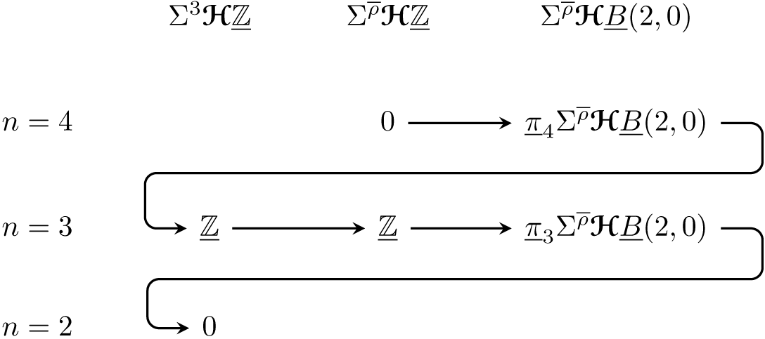
Since $\underline {B}(2,0)$
vanishes at the underlying level, the underlying level of the map
$\underline {B}(2,0)$
vanishes at the underlying level, the underlying level of the map $\underline {\mathbb{Z}} \to \underline {\mathbb{Z}}$
must be an isomorphism. Because these are constant Mackey functors, this determines the homomorphism
$\underline {\mathbb{Z}} \to \underline {\mathbb{Z}}$
must be an isomorphism. Because these are constant Mackey functors, this determines the homomorphism $\underline {\mathbb{Z}} \to \underline {\mathbb{Z}}$
entirely; it must be an isomorphism. Hence,
$\underline {\mathbb{Z}} \to \underline {\mathbb{Z}}$
entirely; it must be an isomorphism. Hence, $\underline {\pi }_3 \Sigma ^{\overline {\rho }} \boldsymbol{\mathscr{H}} \underline {B}(2,0)$
and
$\underline {\pi }_3 \Sigma ^{\overline {\rho }} \boldsymbol{\mathscr{H}} \underline {B}(2,0)$
and $\underline {\pi }_4 \Sigma ^{\overline {\rho }} \boldsymbol{\mathscr{H}} \underline {B}(2,0)$
are zero.
$\underline {\pi }_4 \Sigma ^{\overline {\rho }} \boldsymbol{\mathscr{H}} \underline {B}(2,0)$
are zero.
We next turn to the calculation of the $k\overline {\rho }$
-suspensions of
$k\overline {\rho }$
-suspensions of $\boldsymbol{\mathscr{H}} \underline {B}(2,0)$
. Given the calculation of
$\boldsymbol{\mathscr{H}} \underline {B}(2,0)$
. Given the calculation of $\underline {\pi }_n \Sigma ^{\overline {\rho }} \boldsymbol{\mathscr{H}} \underline {B}(2,0)$
in the previous paragraph, there is a Postnikov sequence
$\underline {\pi }_n \Sigma ^{\overline {\rho }} \boldsymbol{\mathscr{H}} \underline {B}(2,0)$
in the previous paragraph, there is a Postnikov sequence
 \begin{equation*} \Sigma ^1 \boldsymbol{\mathscr{H}} \underline {mg} \to \Sigma ^{\overline {\rho }} \boldsymbol{\mathscr{H}} \underline {B}(2,0) \to \boldsymbol{\mathscr{H}} \underline {g}. \end{equation*}
To use this sequence to compute the homotopy of $\Sigma ^{k\overline {\rho }}\underline {B}(2,0)$
, we must first compute the homotopy of
$\Sigma ^{k\overline {\rho }}\underline {B}(2,0)$
, we must first compute the homotopy of $\Sigma ^{1 + (k-1)\overline {\rho }} \boldsymbol{\mathscr{H}} \underline {mg}$
. As in [Reference Guillou and Yarnall5, Proposition 7.4], there is a short exact sequence of Mackey functors
$\Sigma ^{1 + (k-1)\overline {\rho }} \boldsymbol{\mathscr{H}} \underline {mg}$
. As in [Reference Guillou and Yarnall5, Proposition 7.4], there is a short exact sequence of Mackey functors $\phi _{LDR}^*\, \underline {f} \hookrightarrow \underline {mg} \to \underline {g}^2$
, which gives a fibre sequence
$\phi _{LDR}^*\, \underline {f} \hookrightarrow \underline {mg} \to \underline {g}^2$
, which gives a fibre sequence
 \begin{equation*} \Sigma ^1 \boldsymbol{\mathscr{H}} \phi _{LDR}^* \underline {{\mathbb{F}}_2} = \Sigma ^{\overline {\rho }} \boldsymbol{\mathscr{H}} \phi _{LDR}^*\, \underline {f} \to \Sigma ^{\overline {\rho }} \boldsymbol{\mathscr{H}} \underline {mg} \to \Sigma ^{\overline {\rho }} \boldsymbol{\mathscr{H}} \underline {g}^2 = \boldsymbol{\mathscr{H}} \underline {g}^2. \end{equation*}
Suspending again by $\Sigma ^{(k-2)\overline {\rho }}$
gives a fibre sequence
$\Sigma ^{(k-2)\overline {\rho }}$
gives a fibre sequence
 \begin{equation*} \Sigma ^{1 + (k-2)\overline {\rho }} \boldsymbol{\mathscr{H}} \phi _{LDR}^* \underline {{\mathbb{F}}_2} \to \Sigma ^{(k-1) \overline {\rho }} \boldsymbol{\mathscr{H}} \underline {mg} \to \boldsymbol{\mathscr{H}} \underline {g}^2. \end{equation*}
Using (3.5), we may calculate the homotopy of $\Sigma ^{1+(k-2)\overline {\rho }} \boldsymbol{\mathscr{H}} \phi _{LDR}^* \underline {{\mathbb{F}}_2}$
as in the proof of Proposition4.7 (see also Figure 6). Unwinding the cofibre sequences yields the homotopy of
$\Sigma ^{1+(k-2)\overline {\rho }} \boldsymbol{\mathscr{H}} \phi _{LDR}^* \underline {{\mathbb{F}}_2}$
as in the proof of Proposition4.7 (see also Figure 6). Unwinding the cofibre sequences yields the homotopy of $\Sigma ^{\overline {\rho }} \boldsymbol{\mathscr{H}} B(2,0)$
.
$\Sigma ^{\overline {\rho }} \boldsymbol{\mathscr{H}} B(2,0)$
.
We now use the previous results to determine the Mackey functors $\underline {\pi }_n \Sigma ^{k\overline {\rho }} \boldsymbol{\mathscr{HN}}$
for
$\underline {\pi }_n \Sigma ^{k\overline {\rho }} \boldsymbol{\mathscr{HN}}$
for $k \geq 3$
.
$k \geq 3$
.
Theorem 4.13.
For $k \geq 3$
, the nonzero homotopy Mackey functors of
$k \geq 3$
, the nonzero homotopy Mackey functors of $\Sigma ^{k\overline {\rho }} \boldsymbol{\mathscr{H}} N_e^{\mathcal{K}} \mathbb{F}_2$
are
$\Sigma ^{k\overline {\rho }} \boldsymbol{\mathscr{H}} N_e^{\mathcal{K}} \mathbb{F}_2$
are
 \begin{equation*} \underline {\pi }_n \Sigma ^{k\overline {\rho }} \boldsymbol{\mathscr{H}} N_e^{\mathcal{K}} \mathbb{F}_2 \cong \begin{cases} \underline {\pi }_n \Sigma ^{k\overline {\rho }} \boldsymbol{\mathscr{H}} \underline {\mathbb{F}}_2 & n \geq k+2 \\ \underline {g}^{2k-3} & n=k+1 \\ \phi _{LDR}^* \underline {\mathbb{F}}_2 \oplus \underline {g}^{2k-5} & n=k \\ \underline {g}^{2n-2} & n\in [3,k-1] \\ \underline {g}^3 & n=2 \\ \underline {g} & n=0. \end{cases} \end{equation*}
Proof.
The homotopy Mackey functors in dimensions 0, 1, and 2 are given by Proposition4.7. Those in dimensions at least $k+1$
are given by Corollary4.10. The answer is stated differently here to emphasize the relation to
$k+1$
are given by Corollary4.10. The answer is stated differently here to emphasize the relation to $\Sigma ^{k\overline {\rho }} \boldsymbol{\mathscr{H}} \underline {{\mathbb{F}}_2}$
. These spectra are related via the cofibre sequence
$\Sigma ^{k\overline {\rho }} \boldsymbol{\mathscr{H}} \underline {{\mathbb{F}}_2}$
. These spectra are related via the cofibre sequence
 \begin{equation} \Sigma ^{k\overline {\rho }} \boldsymbol{\mathscr{H}} \underline {B}(2,0) \oplus \underline {g}^2 \to \Sigma ^{k\overline {\rho }} \boldsymbol{\mathscr{HN}} \to \Sigma ^{k\overline {\rho }} \boldsymbol{\mathscr{H}} \underline {{\mathbb{F}}_2}. \end{equation}
By Proposition4.12, the map $\Sigma ^{k\overline {\rho }} \boldsymbol{\mathscr{HN}} \to \Sigma ^{k\overline {\rho }} \boldsymbol{\mathscr{H}} \underline {{\mathbb{F}}_2}$
induces an isomorphism of homotopy Mackey functors in degrees at least
$\Sigma ^{k\overline {\rho }} \boldsymbol{\mathscr{HN}} \to \Sigma ^{k\overline {\rho }} \boldsymbol{\mathscr{H}} \underline {{\mathbb{F}}_2}$
induces an isomorphism of homotopy Mackey functors in degrees at least $k+2$
. In fact, we claim that it is an injection in all degrees. Consider, for instance the long exact sequence associated with (4.14) for
$k+2$
. In fact, we claim that it is an injection in all degrees. Consider, for instance the long exact sequence associated with (4.14) for $k=3$
, where the only Mackey functor remaining to be determined is
$k=3$
, where the only Mackey functor remaining to be determined is $\underline {\pi }_3 \Sigma ^{3\overline {\rho }} \boldsymbol{\mathscr{HN}}$
.
$\underline {\pi }_3 \Sigma ^{3\overline {\rho }} \boldsymbol{\mathscr{HN}}$
.
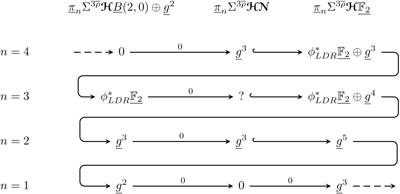
The connecting homomorphism $\underline {\pi }_4 \Sigma ^{3\overline {\rho }} \boldsymbol{\mathscr{H}} \underline {{\mathbb{F}}_2} \to \underline {\pi }_3 \boldsymbol{\mathscr{H}} \underline {B}(2,0) \oplus \underline {g}^2$
is an isomorphism upon restricting to any
$\underline {\pi }_4 \Sigma ^{3\overline {\rho }} \boldsymbol{\mathscr{H}} \underline {{\mathbb{F}}_2} \to \underline {\pi }_3 \boldsymbol{\mathscr{H}} \underline {B}(2,0) \oplus \underline {g}^2$
is an isomorphism upon restricting to any $C_2$
, which forces it to be a surjection of Mackey functors. Thus,
$C_2$
, which forces it to be a surjection of Mackey functors. Thus, $\underline {\pi }_3 \Sigma ^{3\overline {\rho }} \boldsymbol{\mathscr{HN}}$
is a sub-Mackey functor of
$\underline {\pi }_3 \Sigma ^{3\overline {\rho }} \boldsymbol{\mathscr{HN}}$
is a sub-Mackey functor of $\underline {\pi }_3 \Sigma ^{3\overline {\rho }} \boldsymbol{\mathscr{H}} \underline {{\mathbb{F}}_2} \cong \phi _{LDR}^* \underline {{\mathbb{F}}_2} \oplus \underline {g}^4$
. On the other hand, the sequence (4.11) forces a short exact sequence
$\underline {\pi }_3 \Sigma ^{3\overline {\rho }} \boldsymbol{\mathscr{H}} \underline {{\mathbb{F}}_2} \cong \phi _{LDR}^* \underline {{\mathbb{F}}_2} \oplus \underline {g}^4$
. On the other hand, the sequence (4.11) forces a short exact sequence
 \begin{equation*} \underline {g} \hookrightarrow \underline {\pi }_3 \Sigma ^{3\overline {\rho }}\boldsymbol{\mathscr{HN}} \twoheadrightarrow \phi _{LDR}^* \underline {{\mathbb{F}}_2} \end{equation*}
This combines to force an isomorphism $ \underline {\pi }_3 \Sigma ^{3\overline {\rho }} \boldsymbol{\mathscr{HN}} \cong \phi _{LDR}^* \underline {{\mathbb{F}}_2} \oplus \underline {g}$
. A similar argument works for higher values of
$ \underline {\pi }_3 \Sigma ^{3\overline {\rho }} \boldsymbol{\mathscr{HN}} \cong \phi _{LDR}^* \underline {{\mathbb{F}}_2} \oplus \underline {g}$
. A similar argument works for higher values of $k$
.
$k$
.
Remark 4.15.
We argued that the map $\Sigma ^{k\overline {\rho }}\boldsymbol{\mathscr{HN}} \to \Sigma ^{k\overline {\rho }} \boldsymbol{\mathscr{H}} \underline {{\mathbb{F}}_2}$
induces an isomorphism on Mackey functors in degrees at least
$\Sigma ^{k\overline {\rho }}\boldsymbol{\mathscr{HN}} \to \Sigma ^{k\overline {\rho }} \boldsymbol{\mathscr{H}} \underline {{\mathbb{F}}_2}$
induces an isomorphism on Mackey functors in degrees at least $k+2$
by showing that the fibre in(4.14) has no homotopy above degree
$k+2$
by showing that the fibre in(4.14) has no homotopy above degree $k$
, in Proposition
4.12
. In other words, we used that the homology of
$k$
, in Proposition
4.12
. In other words, we used that the homology of $S^{k\overline {\rho }}$
with coefficients in
$S^{k\overline {\rho }}$
with coefficients in $\underline {B}(2,0) \oplus \underline {g}^2$
vanishes above degree
$\underline {B}(2,0) \oplus \underline {g}^2$
vanishes above degree $k$
. An alternative argument for this is that
$k$
. An alternative argument for this is that $S^{k\overline {\rho }}$
has a
$S^{k\overline {\rho }}$
has a $\mathcal{K}$
-CW structure in which all cells in degrees
$\mathcal{K}$
-CW structure in which all cells in degrees $k+1$
or higher are
$k+1$
or higher are $\mathcal{K}$
-free. In particular, it is the
$\mathcal{K}$
-free. In particular, it is the $\mathcal{K}$
-CW structure associated to the
$\mathcal{K}$
-CW structure associated to the $k$
-fold smash product
$k$
-fold smash product $\left (S^{\overline {\rho }}\right )^{\wedge k} \simeq S^{k\overline {\rho }}$
. We need only observe that
$\left (S^{\overline {\rho }}\right )^{\wedge k} \simeq S^{k\overline {\rho }}$
. We need only observe that ${\mathcal{K}}/H \times {\mathcal{K}}/J \cong {\mathcal{K}}/e$
for any two distinct order two subgroups
${\mathcal{K}}/H \times {\mathcal{K}}/J \cong {\mathcal{K}}/e$
for any two distinct order two subgroups $H$
and
$H$
and $J$
. Since
$J$
. Since $ \underline {B}(2,0) \oplus \underline {g}^2$
vanishes at the underlying level, the homology of
$ \underline {B}(2,0) \oplus \underline {g}^2$
vanishes at the underlying level, the homology of $S^{k\overline {\rho }}$
with these coefficients will vanish in degrees at least
$S^{k\overline {\rho }}$
with these coefficients will vanish in degrees at least $k+1$
.
$k+1$
.
The blue shading in the fourth quadrant in Figures 9 and 11 highlights the regions in which the isomorphism $\underline {\pi }_n \Sigma ^{k\overline {\rho }} \boldsymbol{\mathscr{HN}} \cong \underline {\pi }_n \Sigma ^{k\overline {\rho }} \boldsymbol{\mathscr{H}} \underline {{\mathbb{F}}_2}$
was shown to hold in the positive cones.
$\underline {\pi }_n \Sigma ^{k\overline {\rho }} \boldsymbol{\mathscr{HN}} \cong \underline {\pi }_n \Sigma ^{k\overline {\rho }} \boldsymbol{\mathscr{H}} \underline {{\mathbb{F}}_2}$
was shown to hold in the positive cones.
4.2.
The negative cone of
$\boldsymbol{\mathscr{H}} N_e^{{\mathcal{K}}} \mathbb{F}_2$

We now turn to the case of $\Sigma ^{k\overline {\rho }} \boldsymbol{\mathscr{H}} N_e^{{\mathcal{K}}} \mathbb{F}_2$
for
$\Sigma ^{k\overline {\rho }} \boldsymbol{\mathscr{H}} N_e^{{\mathcal{K}}} \mathbb{F}_2$
for $k$
negative. The strategy is largely the same as in Subsection 4.1: most of the answer follows easily from a cofibre sequence, while some extension problems are resolved by considering a separate cofibre sequence.
$k$
negative. The strategy is largely the same as in Subsection 4.1: most of the answer follows easily from a cofibre sequence, while some extension problems are resolved by considering a separate cofibre sequence.
We will again use the Mackey functor $\underline {B}(2,0)$
. An argument as in the proof of Proposition4.12 gives the following computation.
$\underline {B}(2,0)$
. An argument as in the proof of Proposition4.12 gives the following computation.
Proposition 4.16.
The nonzero homotopy Mackey functors of $\Sigma ^{-\overline {\rho }} \boldsymbol{\mathscr{H}} \underline {B}(2,0) \oplus \underline {g}^2$
are
$\Sigma ^{-\overline {\rho }} \boldsymbol{\mathscr{H}} \underline {B}(2,0) \oplus \underline {g}^2$
are
 \begin{equation*} \underline {\pi }_n \Sigma ^{-\overline {\rho }} \boldsymbol{\mathscr{H}} \underline {B}(2,0) \oplus \underline {g}^2 \cong \begin{cases} \underline {g}^3 & n=0 \\ \underline {mg}^* & n=-1. \end{cases} \end{equation*}
For $k \geq 2$
, the nonzero homotopy Mackey functors of
$k \geq 2$
, the nonzero homotopy Mackey functors of $\Sigma ^{-k\overline {\rho }} \boldsymbol{\mathscr{H}} \underline {B}(2,0) \oplus \underline {g}^2$
are
$\Sigma ^{-k\overline {\rho }} \boldsymbol{\mathscr{H}} \underline {B}(2,0) \oplus \underline {g}^2$
are
 \begin{equation*} \underline {\pi }_n \Sigma ^{k\overline {\rho }} \boldsymbol{\mathscr{H}} \underline {B}(2,0) \oplus \underline {g}^2 \cong \begin{cases} \underline {g}^3 & n=0 \\ \underline {g}^2 & n=-1 \\ \underline {g}^3 & n \in [-k+1,-2] \\ \phi _{LDR}^* \underline {\mathbb{F}}_2^* & n=-k. \end{cases} \end{equation*}
Remark 4.17.
Rather than arguing as in Proposition
4.12
, an alternative method to obtain Proposition
4.16
is to use Brown-Comenetz duality, as in [Reference Slone19, Section 8], since the Mackey functors $\underline {B}(2,0)$
and
$\underline {B}(2,0)$
and $\underline {g}$
are self-dual.
$\underline {g}$
are self-dual.
Returning to $\Sigma ^{-k\overline {\rho }} \boldsymbol{\mathscr{HN}}$
, the lower homotopy groups are captured by suspensions of
$\Sigma ^{-k\overline {\rho }} \boldsymbol{\mathscr{HN}}$
, the lower homotopy groups are captured by suspensions of $\boldsymbol{\mathscr{H}} \underline {{\mathbb{F}}_2}$
, as we now describe (see also Figure 4). In Figures 9 and 11, we use red shading in the second quadrant to indicate the region of the negative cone where
$\boldsymbol{\mathscr{H}} \underline {{\mathbb{F}}_2}$
, as we now describe (see also Figure 4). In Figures 9 and 11, we use red shading in the second quadrant to indicate the region of the negative cone where $\pi _{n+k\overline {\rho }} \boldsymbol{\mathscr{H}} \underline {{\mathbb{F}}_2}$
and
$\pi _{n+k\overline {\rho }} \boldsymbol{\mathscr{H}} \underline {{\mathbb{F}}_2}$
and $\pi _{n + k \overline {\rho }} \boldsymbol{\mathscr{HN}}$
agree.
$\pi _{n + k \overline {\rho }} \boldsymbol{\mathscr{HN}}$
agree.
The fibre sequence $\underline {\pi }_* \Sigma ^{-4\overline {\rho }} \boldsymbol{\mathscr{H}} \underline {B}(2,0) \oplus \underline {g}^2 \to \underline {\pi }_* \Sigma ^{-4\overline {\rho }} \boldsymbol{\mathscr{HN}} \to \underline {\pi }_* \Sigma ^{-4\overline {\rho }} \boldsymbol{\mathscr{H}} \underline {{\mathbb{F}}_2}$
. In the green (upper left) region, the homotopy of
$\underline {\pi }_* \Sigma ^{-4\overline {\rho }} \boldsymbol{\mathscr{H}} \underline {B}(2,0) \oplus \underline {g}^2 \to \underline {\pi }_* \Sigma ^{-4\overline {\rho }} \boldsymbol{\mathscr{HN}} \to \underline {\pi }_* \Sigma ^{-4\overline {\rho }} \boldsymbol{\mathscr{H}} \underline {{\mathbb{F}}_2}$
. In the green (upper left) region, the homotopy of $\Sigma ^{-4\overline {\rho }}\boldsymbol{\mathscr{HN}}$
matches the homotopy of the fibre, and in the red (lower right) region, the homotopy is the same as the homotopy of
$\Sigma ^{-4\overline {\rho }}\boldsymbol{\mathscr{HN}}$
matches the homotopy of the fibre, and in the red (lower right) region, the homotopy is the same as the homotopy of $\boldsymbol{\mathscr{H}}\underline {{\mathbb{F}}_2}$
.
$\boldsymbol{\mathscr{H}}\underline {{\mathbb{F}}_2}$
.

Proposition 4.18.
The map $\Sigma ^{-k\overline {\rho }} \boldsymbol{\mathscr{H}} N_e^{\mathcal{K}} \mathbb{F}_2 \to \Sigma ^{-k\overline {\rho }} \boldsymbol{\mathscr{H}} \underline {{\mathbb{F}}_2}$
is an isomorphism on
$\Sigma ^{-k\overline {\rho }} \boldsymbol{\mathscr{H}} N_e^{\mathcal{K}} \mathbb{F}_2 \to \Sigma ^{-k\overline {\rho }} \boldsymbol{\mathscr{H}} \underline {{\mathbb{F}}_2}$
is an isomorphism on $\underline {\pi }_n$
for
$\underline {\pi }_n$
for $n \lt -k$
, while the map
$n \lt -k$
, while the map $\Sigma ^{-k\overline {\rho }} \boldsymbol{\mathscr{H}} \underline {B}(2,0) \oplus \underline {g}^2 \to \Sigma ^{-k\overline {\rho }} \boldsymbol{\mathscr{H}} N_e^{\mathcal{K}} \mathbb{F}_2$
is an isomorphism on
$\Sigma ^{-k\overline {\rho }} \boldsymbol{\mathscr{H}} \underline {B}(2,0) \oplus \underline {g}^2 \to \Sigma ^{-k\overline {\rho }} \boldsymbol{\mathscr{H}} N_e^{\mathcal{K}} \mathbb{F}_2$
is an isomorphism on $\underline {\pi }_n$
for
$\underline {\pi }_n$
for $n\in \{0,-1,-2\}$
.
$n\in \{0,-1,-2\}$
.
Proof. This follows from the cofibre sequence
 \begin{equation*} \Sigma ^{-k\overline {\rho }} \boldsymbol{\mathscr{H}} \underline {B}(2,0) \oplus \underline {g}^2 \to \Sigma ^{-k\overline {\rho }} \boldsymbol{\mathscr{HN}} \to \Sigma ^{-k\overline {\rho }} \boldsymbol{\mathscr{H}} \underline {{\mathbb{F}}_2}, \end{equation*}
together with the fact that $\Sigma ^{-k\overline {\rho }} \boldsymbol{\mathscr{H}} \underline {B}(2,0) \oplus \underline {g}^2$
is
$\Sigma ^{-k\overline {\rho }} \boldsymbol{\mathscr{H}} \underline {B}(2,0) \oplus \underline {g}^2$
is $-k$
-connective and
$-k$
-connective and $\Sigma ^{-k\overline {\rho }} \boldsymbol{\mathscr{H}} \underline {{\mathbb{F}}_2} \simeq \Sigma ^{-3-(k-1)\overline {\rho }} \boldsymbol{\mathscr{H}} \underline {{\mathbb{F}}_2}^*$
has no homotopy above dimension
$\Sigma ^{-k\overline {\rho }} \boldsymbol{\mathscr{H}} \underline {{\mathbb{F}}_2} \simeq \Sigma ^{-3-(k-1)\overline {\rho }} \boldsymbol{\mathscr{H}} \underline {{\mathbb{F}}_2}^*$
has no homotopy above dimension $-3$
.
$-3$
.
Note that Proposition4.18 captures all of the homotopy groups in the case of $-k$
equal to either
$-k$
equal to either $-1$
or
$-1$
or $-2$
. The remaining cases are described in the next result.
$-2$
. The remaining cases are described in the next result.
Theorem 4.19.
For $-k\leq -3$
, the nonzero homotopy Mackey functors of
$-k\leq -3$
, the nonzero homotopy Mackey functors of $\Sigma ^{-k\overline {\rho }} \boldsymbol{\mathscr{H}} N_e^{\mathcal{K}} \mathbb{F}_2$
are
$\Sigma ^{-k\overline {\rho }} \boldsymbol{\mathscr{H}} N_e^{\mathcal{K}} \mathbb{F}_2$
are
 \begin{equation*} \underline {\pi }_n \Sigma ^{-k\overline {\rho }} \boldsymbol{\mathscr{H}} N_e^{\mathcal{K}} \mathbb{F}_2 \cong \begin{cases} \underline {g}^3 & n=0 \\ \underline {g}^2 & n=-1 \\ \underline {g}^3 & n=-2 \\ \underline {g}^{-2n-2} & n\in [-k+1,-3] \\ \phi _{LDR}^* \underline {{\mathbb{F}}_2}^* \oplus \underline {g}^{2k-5} & n=-k \\ \underline {\pi }_n \Sigma ^{-k\overline {\rho }} \boldsymbol{\mathscr{H}} \underline {\mathbb{F}}_2 & n \leq -k-1. \end{cases} \end{equation*}
Proof.
By Proposition4.18, it remains to capture the homotopy in degrees $n\in [-k,-3]$
. The Mackey functors listed here are the only possibilities that are simultaneously compatible with the fibre sequence
$n\in [-k,-3]$
. The Mackey functors listed here are the only possibilities that are simultaneously compatible with the fibre sequence
 \begin{equation*} \Sigma ^{-k\overline {\rho }} \boldsymbol{\mathscr{H}} \underline {B}(2,0) \oplus \underline {g}^2 \to \Sigma ^{-k\overline {\rho }} \boldsymbol{\mathscr{HN}} \to \Sigma ^{-k\overline {\rho }} \boldsymbol{\mathscr{H}} \underline {{\mathbb{F}}_2}, \end{equation*}
as well as the fibre sequence
 \begin{equation*} \Sigma ^{-k\overline {\rho }} \boldsymbol{\mathscr{H}} \underline {{\mathbb{F}}_2}^* \to \Sigma ^{-k\overline {\rho }} \boldsymbol{\mathscr{HN}} \to \Sigma ^{-k\overline {\rho }} \boldsymbol{\mathscr{H}} \underline {E}. \end{equation*}
For example, in the case $k=3$
, the first fibre sequence provides the short exact sequence
$k=3$
, the first fibre sequence provides the short exact sequence
 \begin{equation*} \phi _{LDR}^* \underline {{\mathbb{F}}_2}^* \hookrightarrow \underline {\pi }_{-3} \Sigma ^{-3\overline {\rho }} \boldsymbol{\mathscr{HN}} \twoheadrightarrow \underline {g}, \end{equation*}
while the second provides the short exact sequence
 \begin{equation*} \underline {g}^3 \hookrightarrow \phi _{LDR}^* \underline {{\mathbb{F}}_2}^* \oplus \underline {g}^4 \twoheadrightarrow \underline {\pi }_{-3} \Sigma ^{-3\overline {\rho }} \boldsymbol{\mathscr{HN}}. \end{equation*}
It follows that $\underline {\pi }_{-3} \Sigma ^{-3\overline {\rho }} \boldsymbol{\mathscr{HN}}$
must be
$\underline {\pi }_{-3} \Sigma ^{-3\overline {\rho }} \boldsymbol{\mathscr{HN}}$
must be $\phi _{LDR}^* \underline {{\mathbb{F}}_2}^* \oplus \underline {g}$
.
$\phi _{LDR}^* \underline {{\mathbb{F}}_2}^* \oplus \underline {g}$
.
Remark 4.20.
Dual to the proof of Theorem
4.13
, here the map $\underline {\pi }_n \Sigma ^{-k\overline {\rho }} \boldsymbol{\mathscr{H}} \underline {{\mathbb{F}}_2}^* \to \underline {\pi }_n \Sigma ^{-k\overline {\rho }} \boldsymbol{\mathscr{H}} N_e^{\mathcal{K}} \mathbb{F}_2$
is surjective for
$\underline {\pi }_n \Sigma ^{-k\overline {\rho }} \boldsymbol{\mathscr{H}} \underline {{\mathbb{F}}_2}^* \to \underline {\pi }_n \Sigma ^{-k\overline {\rho }} \boldsymbol{\mathscr{H}} N_e^{\mathcal{K}} \mathbb{F}_2$
is surjective for $k\lt 0$
.
$k\lt 0$
.
The homotopy $\underline {\pi }_{n + k\overline {\rho }}\boldsymbol{\mathscr{HN}} = \underline {\pi }_{n + k \overline {\rho }}\boldsymbol{\mathscr{H}} N_e^{\mathcal{K}} \mathbb{F}_2$
is displayed in Figure 11.
$\underline {\pi }_{n + k\overline {\rho }}\boldsymbol{\mathscr{HN}} = \underline {\pi }_{n + k \overline {\rho }}\boldsymbol{\mathscr{H}} N_e^{\mathcal{K}} \mathbb{F}_2$
is displayed in Figure 11.
5. The homotopy of
$\boldsymbol{\mathscr{H}} N_D^K \mathbb{F}_2$

We compute the homotopy Mackey functors $\underline {\pi }^{\mathcal{K}}_{n+k\overline {\rho }}(\boldsymbol{\mathscr{HN}}_{\!D})$
, where
$\underline {\pi }^{\mathcal{K}}_{n+k\overline {\rho }}(\boldsymbol{\mathscr{HN}}_{\!D})$
, where $\boldsymbol{\mathscr{N}}_{\!D} = N_D^{\mathcal{K}} \underline {{\mathbb{F}}_2}$
. The Tambara functor structure of
$\boldsymbol{\mathscr{N}}_{\!D} = N_D^{\mathcal{K}} \underline {{\mathbb{F}}_2}$
. The Tambara functor structure of $\boldsymbol{\mathscr{N}}_{\!D}$
is displayed in Figure 3. As in the previous section, we first compute the positive cone.
$\boldsymbol{\mathscr{N}}_{\!D}$
is displayed in Figure 3. As in the previous section, we first compute the positive cone.
5.1.
The positive cone of
$\boldsymbol{\mathscr{H}} N_D^{{\mathcal{K}}} \_ {{\mathbb{F}}_2}$

We compute the homotopy Mackey functors of the $\mathcal{K}$
-spectra
$\mathcal{K}$
-spectra $\Sigma ^{k\overline {\rho }} \boldsymbol{\mathscr{HN}}_{\!D}$
. As usual, we begin with a short exact sequence of Mackey functors.
$\Sigma ^{k\overline {\rho }} \boldsymbol{\mathscr{HN}}_{\!D}$
. As usual, we begin with a short exact sequence of Mackey functors.
Let us write $\overline {\boldsymbol{\mathscr{N}}_{\!D}}$
for the sub-Mackey functor of
$\overline {\boldsymbol{\mathscr{N}}_{\!D}}$
for the sub-Mackey functor of $\boldsymbol{\mathscr{N}}_{\!D}$
generated at the proper subgroups, as displayed in Figure 5. We then have a short exact sequence
$\boldsymbol{\mathscr{N}}_{\!D}$
generated at the proper subgroups, as displayed in Figure 5. We then have a short exact sequence
 \begin{equation} \overline {\boldsymbol{\mathscr{N}}_{\!D}} \hookrightarrow \boldsymbol{\mathscr{N}}_{\!D} \twoheadrightarrow \underline {g}. \end{equation}
Furthermore, we have a short exact sequence of Mackey functors
 \begin{equation} \underline {v}_D^* \hookrightarrow \overline {\boldsymbol{\mathscr{N}}_{\!D}} \twoheadrightarrow \varphi ^*_D \mathbb{F}_2^* \oplus \underline {n}_D^*, \end{equation}
where $\underline {v}_D^*$
is as described in Table 4.
$\underline {v}_D^*$
is as described in Table 4.
The $\mathcal{K}$
-Mackey functor
$\mathcal{K}$
-Mackey functor $\overline {\boldsymbol{\mathscr{N}}_{\!D}} =\overline {N_D^{\mathcal{K}} \underline {{\mathbb{F}}_2}}$
, which is the kernel of the augmentation
$\overline {\boldsymbol{\mathscr{N}}_{\!D}} =\overline {N_D^{\mathcal{K}} \underline {{\mathbb{F}}_2}}$
, which is the kernel of the augmentation $N_D^{\mathcal{K}}(\underline {{\mathbb{F}}_2}) \to \underline {g}$
.
$N_D^{\mathcal{K}}(\underline {{\mathbb{F}}_2}) \to \underline {g}$
.

Proposition 5.3.
There is an equivalence $\Sigma ^{\overline {\rho }} \boldsymbol{\mathscr{H}} \underline {n}_D^* \simeq \Sigma ^1 \boldsymbol{\mathscr{H}} \underline {n}_D$
.
$\Sigma ^{\overline {\rho }} \boldsymbol{\mathscr{H}} \underline {n}_D^* \simeq \Sigma ^1 \boldsymbol{\mathscr{H}} \underline {n}_D$
.
Proof.
First, note that since $\underline {n}_D^*$
restricts to zero on
$\underline {n}_D^*$
restricts to zero on $D$
, it follows that the natural map
$D$
, it follows that the natural map $\boldsymbol{\mathscr{H}} \underline {n}_D^* \to \Sigma ^{\sigma _D} \boldsymbol{\mathscr{H}} \underline {n}_D^*$
is an equivalence by Corollary3.3. The cofibre sequence
$\boldsymbol{\mathscr{H}} \underline {n}_D^* \to \Sigma ^{\sigma _D} \boldsymbol{\mathscr{H}} \underline {n}_D^*$
is an equivalence by Corollary3.3. The cofibre sequence
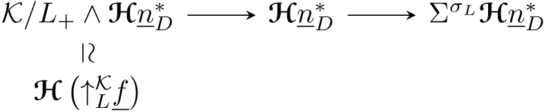
allows us compute the homotopy Mackey functors of $\Sigma ^{\sigma _L} \boldsymbol{\mathscr{H}} \underline {n}_D^* \simeq \Sigma ^{\sigma _L+\sigma _D} \boldsymbol{\mathscr{H}} \underline {n}_D^*$
; the nonzero homotopy Mackey functors are
$\Sigma ^{\sigma _L} \boldsymbol{\mathscr{H}} \underline {n}_D^* \simeq \Sigma ^{\sigma _L+\sigma _D} \boldsymbol{\mathscr{H}} \underline {n}_D^*$
; the nonzero homotopy Mackey functors are $\phi _L^*\, \underline {f}$
in degree one and
$\phi _L^*\, \underline {f}$
in degree one and $\phi _R^*\, \underline {f}$
in degree zero. This gives a Postnikov fibre sequence
$\phi _R^*\, \underline {f}$
in degree zero. This gives a Postnikov fibre sequence
 \begin{equation*} \Sigma ^1 \boldsymbol{\mathscr{H}} \phi _L^*\, \underline {f} \to \Sigma ^{\sigma _L+\sigma _D} \boldsymbol{\mathscr{H}} \underline {n}_D^* \to \boldsymbol{\mathscr{H}} \phi _R^*\, \underline {f}. \end{equation*}
Suspending by $\sigma _R$
then gives a fibre sequence
$\sigma _R$
then gives a fibre sequence

where we have again used the fact that if the restriction of $X$
to
$X$
to $R$
is contractible, then
$R$
is contractible, then $\Sigma ^{\sigma _R}X \simeq X$
(Corollary3.3). It follows that
$\Sigma ^{\sigma _R}X \simeq X$
(Corollary3.3). It follows that $\Sigma ^{\overline {\rho }} \boldsymbol{\mathscr{H}} \underline {n}_D^*$
has homotopy concentrated in degree 1, with Mackey functor an extension of
$\Sigma ^{\overline {\rho }} \boldsymbol{\mathscr{H}} \underline {n}_D^*$
has homotopy concentrated in degree 1, with Mackey functor an extension of $\phi _R^* \underline {{\mathbb{F}}_2}$
by
$\phi _R^* \underline {{\mathbb{F}}_2}$
by $\phi _L^*\, \underline {f}$
. The only potential ambiguity in the extension is the restriction from
$\phi _L^*\, \underline {f}$
. The only potential ambiguity in the extension is the restriction from $K$
to
$K$
to $L$
. But as the result must be symmetric in
$L$
. But as the result must be symmetric in $L$
and
$L$
and $R$
, we conclude the restriction to
$R$
, we conclude the restriction to $L$
must be nontrivial since the restriction to
$L$
must be nontrivial since the restriction to $R$
is so. Hence, this extension must be
$R$
is so. Hence, this extension must be $\underline {n}_D^*$
.
$\underline {n}_D^*$
.
Proposition 5.4.
For $k\geq 1$
, the nonzero homotopy Mackey functors of
$k\geq 1$
, the nonzero homotopy Mackey functors of $\Sigma ^{k\overline {\rho }} \boldsymbol{\mathscr{H}} \underline {n}_D$
are
$\Sigma ^{k\overline {\rho }} \boldsymbol{\mathscr{H}} \underline {n}_D$
are
 \begin{equation*} \underline {\pi }_n \Sigma ^{k\overline {\rho }} \boldsymbol{\mathscr{H}}\underline {n}_D \cong \begin{cases} \phi _{LR}^* \underline {{\mathbb{F}}_2} & n= k \\ \underline {g}^2 & n \in [1,k-1] \\ \underline {g} & n=0. \end{cases} \end{equation*}
Proof.
We have a short exact sequence of Mackey functors $\phi _{LR}^*\, \underline {f} \hookrightarrow \underline {n}_D \twoheadrightarrow \underline {g}$
. Suspending by
$\phi _{LR}^*\, \underline {f} \hookrightarrow \underline {n}_D \twoheadrightarrow \underline {g}$
. Suspending by $\overline {\rho }$
and use of Proposition3.6 give a cofibre sequence
$\overline {\rho }$
and use of Proposition3.6 give a cofibre sequence

The homotopy of the higher $\overline {\rho }$
-suspensions follow by use of (3.5) from the relevant
$\overline {\rho }$
-suspensions follow by use of (3.5) from the relevant $C_2$
-equivariant computations, as in Figure 3.
$C_2$
-equivariant computations, as in Figure 3.
Recall that $\underline {v}_D^*$
fits into a short exact sequence (5.2) with middle term
$\underline {v}_D^*$
fits into a short exact sequence (5.2) with middle term $\overline {\boldsymbol{\mathscr{N}}_{\!D}}$
. Understanding its homotopy will be crucial for computing the homotopy of
$\overline {\boldsymbol{\mathscr{N}}_{\!D}}$
. Understanding its homotopy will be crucial for computing the homotopy of $\overline {\boldsymbol{\mathscr{N}}_{\!D}}$
, which we use in turn to compute the homotopy of
$\overline {\boldsymbol{\mathscr{N}}_{\!D}}$
, which we use in turn to compute the homotopy of $\boldsymbol{\mathscr{N}}_{\!D}$
.
$\boldsymbol{\mathscr{N}}_{\!D}$
.
Proposition 5.5.
The nonzero homotopy Mackey functors of $\Sigma ^{\overline {\rho }} \boldsymbol{\mathscr{H}} \underline {v}_D^*$
are
$\Sigma ^{\overline {\rho }} \boldsymbol{\mathscr{H}} \underline {v}_D^*$
are
 \begin{equation*} \underline {\pi }_n \Sigma ^{\overline {\rho }} \boldsymbol{\mathscr{H}}\underline {v}_D^* \cong \begin{cases} \underline {{\mathbb{F}}_2} & n=3 \\ \phi _D^*\, \underline {f} & n=2. \\ \end{cases} \end{equation*}
For $k\geq 2$
, the nonzero homotopy Mackey functors of
$k\geq 2$
, the nonzero homotopy Mackey functors of $\Sigma ^{k\overline {\rho }} \boldsymbol{\mathscr{H}} \underline {v}_D^*$
are
$\Sigma ^{k\overline {\rho }} \boldsymbol{\mathscr{H}} \underline {v}_D^*$
are
 \begin{equation*} \underline {\pi }_n \Sigma ^{k\overline {\rho }} \boldsymbol{\mathscr{H}}\underline {v}_D^* \cong \begin{cases} \underline {\pi }_n \Sigma ^{k\overline {\rho }} \boldsymbol{\mathscr{H}} \mathbb{F}_2 & n \geq k+2 \\ \phi _D^* \underline {{\mathbb{F}}_2} \oplus \underline {g}^{2k-3} & n=k+1 \\ \underline {g}^{2n-4} & n \in [3,k]. \\ \end{cases} \end{equation*}
Proof.
We have a short exact sequence $\phi _D^* \underline {{\mathbb{F}}_2}^* \hookrightarrow \underline {{\mathbb{F}}_2}^* \twoheadrightarrow \underline {v}_D^*$
, which gives rise to a cofibre sequence
$\phi _D^* \underline {{\mathbb{F}}_2}^* \hookrightarrow \underline {{\mathbb{F}}_2}^* \twoheadrightarrow \underline {v}_D^*$
, which gives rise to a cofibre sequence
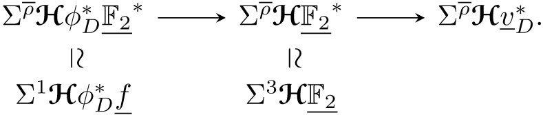
We may rotate this and suspend further to get a cofibre sequence
 \begin{equation*} \Sigma ^{3+(k-1)\overline {\rho }} \boldsymbol{\mathscr{H}} \underline {{\mathbb{F}}_2} \to \Sigma ^{k\overline {\rho }} \boldsymbol{\mathscr{H}} \underline {v}_D^* \to \Sigma ^{2+(k-2)\overline {\rho }}\boldsymbol{\mathscr{H}} \phi _D^* \underline {{\mathbb{F}}_2}. \end{equation*}
The homotopy Mackey functors of suspensions of $\boldsymbol{\mathscr{H}} \underline {{\mathbb{F}}_2}$
can be read off from Figure 9, and the homotopy Mackey functors of
$\boldsymbol{\mathscr{H}} \underline {{\mathbb{F}}_2}$
can be read off from Figure 9, and the homotopy Mackey functors of $\Sigma ^{2+(k-2)\overline {\rho }}\boldsymbol{\mathscr{H}} \phi _D^* \underline {{\mathbb{F}}_2}$
follow from (3.5) and Figure 6.
$\Sigma ^{2+(k-2)\overline {\rho }}\boldsymbol{\mathscr{H}} \phi _D^* \underline {{\mathbb{F}}_2}$
follow from (3.5) and Figure 6.
On the other hand, we also have a short exact sequence $\phi _{LR}^*\, \underline {f} \hookrightarrow \underline {v}_D^* \twoheadrightarrow \underline {f}$
which gives a cofibre sequence
$\phi _{LR}^*\, \underline {f} \hookrightarrow \underline {v}_D^* \twoheadrightarrow \underline {f}$
which gives a cofibre sequence

The homotopy Mackey functors of the right term of this last cofibre sequence are computed in [Reference Guillou and Yarnall5, Corollary 7.5], and the homotopy Mackey functors of $\Sigma ^{1+(k-1)\overline {\rho }} \boldsymbol{\mathscr{H}} \phi _{LR}^* \underline {{\mathbb{F}}_2}$
follow from (3.5) and Figure 6. The stated homotopy Mackey functors of
$\Sigma ^{1+(k-1)\overline {\rho }} \boldsymbol{\mathscr{H}} \phi _{LR}^* \underline {{\mathbb{F}}_2}$
follow from (3.5) and Figure 6. The stated homotopy Mackey functors of $\Sigma ^{k \overline {\rho }} \boldsymbol{\mathscr{H}} \underline {v}_D^*$
are the only ones compatible with both long exact sequences and Lemma2.17.
$\Sigma ^{k \overline {\rho }} \boldsymbol{\mathscr{H}} \underline {v}_D^*$
are the only ones compatible with both long exact sequences and Lemma2.17.
Proposition 5.6.
The nonzero homotopy Mackey functors of $\Sigma ^{\overline {\rho }} \boldsymbol{\mathscr{H}} N_D^{\mathcal{K}} \underline {{\mathbb{F}}_2}$
are
$\Sigma ^{\overline {\rho }} \boldsymbol{\mathscr{H}} N_D^{\mathcal{K}} \underline {{\mathbb{F}}_2}$
are
 \begin{equation*} \underline {\pi }_n \Sigma ^{\overline {\rho }} \boldsymbol{\mathscr{H}} N_D^{\mathcal{K}} \underline {{\mathbb{F}}_2} \cong \begin{cases} \underline {{\mathbb{F}}_2} & n =3 \\ \phi _D^*\, \underline {f} & n=2 \\ \phi _{D}^*\, \underline {f} \oplus \underline {n}_D & n=1 \\ \underline {g} & n=0. \end{cases} \end{equation*}
Proof. Suspending (5.1) gives a cofibre sequence
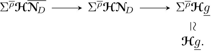
It therefore suffices to compute the homotopy Mackey functors of $\Sigma ^{\overline {\rho }} \boldsymbol{\mathscr{H}} \overline {\boldsymbol{\mathscr{N}}_{\!D}}$
, for which we use the following suspension of (5.2):
$\Sigma ^{\overline {\rho }} \boldsymbol{\mathscr{H}} \overline {\boldsymbol{\mathscr{N}}_{\!D}}$
, for which we use the following suspension of (5.2):
 \begin{equation*} \Sigma ^{\overline {\rho }} \boldsymbol{\mathscr{H}} \underline {v}_D^* \to \Sigma ^{\overline {\rho }} \boldsymbol{\mathscr{H}} \overline {\boldsymbol{\mathscr{N}}_{\!D}} \to \Sigma ^{\overline {\rho }} \boldsymbol{\mathscr{H}} \big ( \phi _D^* \underline {{\mathbb{F}}_2}^* \oplus \underline {n}_D^* \big ). \end{equation*}
The result now follows by combining Propositions3.6, 5.3 and 5.5.
The homotopy of the higher suspensions is as follows.
Theorem 5.7.
For $k\geq 2$
, the nonzero homotopy Mackey functors of
$k\geq 2$
, the nonzero homotopy Mackey functors of $\Sigma ^{k\overline {\rho }} \boldsymbol{\mathscr{H}} N_D^{\mathcal{K}} \underline {{\mathbb{F}}_2}$
are
$\Sigma ^{k\overline {\rho }} \boldsymbol{\mathscr{H}} N_D^{\mathcal{K}} \underline {{\mathbb{F}}_2}$
are
 \begin{equation*} \underline {\pi }_n \Sigma ^{k\overline {\rho }} \boldsymbol{\mathscr{H}} N_D^{\mathcal{K}} \underline {{\mathbb{F}}_2} \cong \begin{cases} \underline {\pi }_n \Sigma ^{k\overline {\rho }} \boldsymbol{\mathscr{H}} \underline {{\mathbb{F}}_2} & n \geq k+2 \\ \phi _D^* \underline {{\mathbb{F}}_2} \oplus \underline {g}^{2k-3} & n=k+1 \\ \phi _{LDR}^* \underline {{\mathbb{F}}_2} \oplus \underline {g}^{2k-4} & n=k \\ \underline {g}^{2n-1} & n \in [2,k-1] \\ \underline {g} & n \in [0,1]. \end{cases} \end{equation*}
Proof. The argument is the same as for Proposition5.6, using the cofibre sequence
 \begin{equation*} \Sigma ^{k\overline {\rho }} \boldsymbol{\mathscr{H}} \underline {v}_D^* \to \Sigma ^{k\overline {\rho }} \boldsymbol{\mathscr{H}} \overline {\boldsymbol{\mathscr{N}}_{\!D}} \to \Sigma ^{k\overline {\rho }} \boldsymbol{\mathscr{H}} \big ( \phi _D^* \underline {{\mathbb{F}}_2}^* \oplus \underline {n}_D^* \big ). \end{equation*}
for $k\geq 2$
. The left term has homotopy in degrees at least 3, while the right term has homotopy in degrees at most
$k\geq 2$
. The left term has homotopy in degrees at least 3, while the right term has homotopy in degrees at most $k$
. Therefore the homotopy Mackey functors in degrees greater than
$k$
. Therefore the homotopy Mackey functors in degrees greater than $k$
follow from Proposition5.5. And the homotopy below degree 3 follows from Proposition5.4.
$k$
follow from Proposition5.5. And the homotopy below degree 3 follows from Proposition5.4.
For the Mackey functors in degrees $k$
and lower, we employ a similar argument to that used in the proof of Theorem4.13. Consider, for instance, the case
$k$
and lower, we employ a similar argument to that used in the proof of Theorem4.13. Consider, for instance, the case $k=4$
, where the Mackey functors
$k=4$
, where the Mackey functors $\underline {\pi }_3$
and
$\underline {\pi }_3$
and $\underline {\pi }_4$
remain to be determined. In the relevant degrees, the long exact sequence arising from the above cofibre sequence takes the form
$\underline {\pi }_4$
remain to be determined. In the relevant degrees, the long exact sequence arising from the above cofibre sequence takes the form
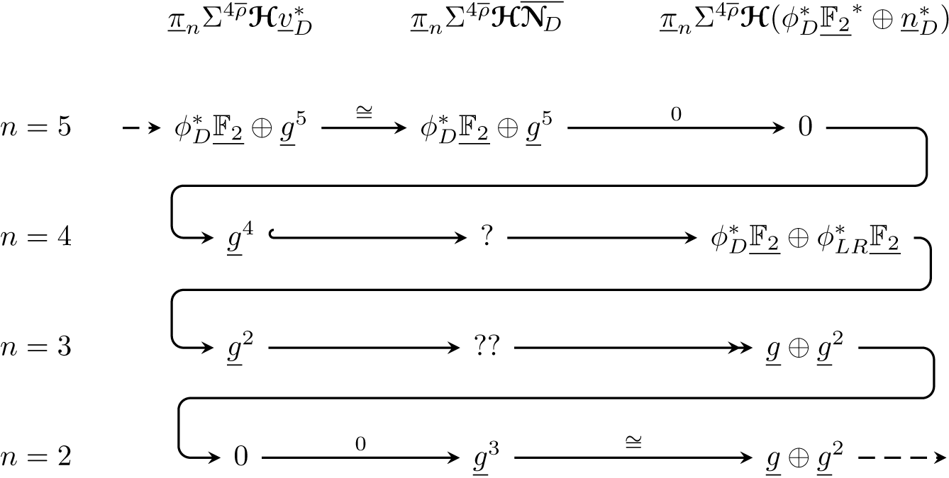
On the other hand, the long exact sequence induced by (the rotation of) the cofibre sequence for $\underline {g} \oplus \underline {n}_D \hookrightarrow \boldsymbol{\mathscr{N}}_{\!D} \twoheadrightarrow \underline {{\mathbb{F}}_2}$
takes the form
$\underline {g} \oplus \underline {n}_D \hookrightarrow \boldsymbol{\mathscr{N}}_{\!D} \twoheadrightarrow \underline {{\mathbb{F}}_2}$
takes the form

The claimed values for $\underline {\pi }_4$
and
$\underline {\pi }_4$
and $\underline {\pi }_3$
are the only possibilities compatible with both long exact sequences. Note that although one sequence computes the homotopy of
$\underline {\pi }_3$
are the only possibilities compatible with both long exact sequences. Note that although one sequence computes the homotopy of $\boldsymbol{\mathscr{N}}_{\!D}$
and the other computes the homotopy of
$\boldsymbol{\mathscr{N}}_{\!D}$
and the other computes the homotopy of $\overline {\boldsymbol{\mathscr{N}}_{\!D}}$
, these agree in positive degree as in the proof of Proposition5.6. The argument works just as well for larger values of
$\overline {\boldsymbol{\mathscr{N}}_{\!D}}$
, these agree in positive degree as in the proof of Proposition5.6. The argument works just as well for larger values of $k$
.
$k$
.
We display these results in the fourth quadrant of Figure 13. The region of the fourth quadrant of Figure 13 where the homotopy agrees with $\boldsymbol{\mathscr{H}} \underline {{\mathbb{F}}_2}$
is highlighted in blue.
$\boldsymbol{\mathscr{H}} \underline {{\mathbb{F}}_2}$
is highlighted in blue.
5.2.
The negative cone of
$\boldsymbol{\mathscr{H}} N_D^{{\mathcal{K}}} \_ {{\mathbb{F}}_2}$

We now compute the negative cone with coefficients in $\boldsymbol{\mathscr{N}}_{\!D} = N_D^{\mathcal{K}} \underline {{\mathbb{F}}_2}$
, which we display in the second quadrant of Figure 13.
$\boldsymbol{\mathscr{N}}_{\!D} = N_D^{\mathcal{K}} \underline {{\mathbb{F}}_2}$
, which we display in the second quadrant of Figure 13.
Proposition 5.8.
The nonzero homotopy Mackey functors of $\Sigma ^{-\overline {\rho }} \boldsymbol{\mathscr{H}} N_D^{\mathcal{K}} \underline {{\mathbb{F}}_2}$
are
$\Sigma ^{-\overline {\rho }} \boldsymbol{\mathscr{H}} N_D^{\mathcal{K}} \underline {{\mathbb{F}}_2}$
are
 \begin{equation*} \underline {\pi }_{-n} \Sigma ^{-\overline {\rho }} \boldsymbol{\mathscr{H}} N_D^{\mathcal{K}} \underline {{\mathbb{F}}_2} \cong \begin{cases} \underline {{\mathbb{F}}_2}^* & n =3 \\ \underline {n}_D^* & n=1 \\ \underline {g} & n=0. \end{cases} \end{equation*}
Proof.
The short exact sequence of Mackey functors $\underline {g} \oplus \underline {n}_D \hookrightarrow \boldsymbol{\mathscr{N}}_{\!D} \twoheadrightarrow \underline {{\mathbb{F}}_2}$
gives a cofibre sequence
$\underline {g} \oplus \underline {n}_D \hookrightarrow \boldsymbol{\mathscr{N}}_{\!D} \twoheadrightarrow \underline {{\mathbb{F}}_2}$
gives a cofibre sequence

according to Proposition5.3. The result follows from the associated long exact sequence.
Theorem 5.9.
For $k\geq 2$
, the nonzero homotopy Mackey functors of
$k\geq 2$
, the nonzero homotopy Mackey functors of $\Sigma ^{-k\overline {\rho }} \boldsymbol{\mathscr{H}} N_D^{\mathcal{K}} \underline {{\mathbb{F}}_2}$
are
$\Sigma ^{-k\overline {\rho }} \boldsymbol{\mathscr{H}} N_D^{\mathcal{K}} \underline {{\mathbb{F}}_2}$
are
 \begin{equation*} \underline {\pi }_{-n} \Sigma ^{-k\overline {\rho }} \boldsymbol{\mathscr{H}} N_D^{\mathcal{K}} \underline {{\mathbb{F}}_2} \cong \begin{cases} \underline {\pi }_{-n} \Sigma ^{-k\overline {\rho }} \boldsymbol{\mathscr{H}} \underline {{\mathbb{F}}_2} & n \geq k+1 \\ \phi _{LR}^* \underline {{\mathbb{F}}_2}^* \oplus \underline {g}^{2k-5} & n=k \\ \underline {g}^{2n-3} & n \in [3,k-1] \\ \underline {g}^2 & n = 2 \\ \underline {g} & n = 0,1. \end{cases} \end{equation*}
Proof. As in the proof of Proposition5.8, we have a cofibre sequence

The homotopy Mackey functors of $\Sigma ^{-k\overline {\rho }} \boldsymbol{\mathscr{H}} \underline {n}_D^*$
are the duals of those given in Proposition5.4 by Brown-Comenetz duality. Thus
$\Sigma ^{-k\overline {\rho }} \boldsymbol{\mathscr{H}} \underline {n}_D^*$
are the duals of those given in Proposition5.4 by Brown-Comenetz duality. Thus $\Sigma ^{-k\overline {\rho }} \boldsymbol{\mathscr{H}} (\underline {g} \oplus \underline {n}_D)$
is
$\Sigma ^{-k\overline {\rho }} \boldsymbol{\mathscr{H}} (\underline {g} \oplus \underline {n}_D)$
is $(\!-\!k)$
-connective, so that the homotopy Mackey functors of
$(\!-\!k)$
-connective, so that the homotopy Mackey functors of $\Sigma ^{-k\overline {\rho }} \boldsymbol{\mathscr{HN}}_{\!D}$
agree with those of
$\Sigma ^{-k\overline {\rho }} \boldsymbol{\mathscr{HN}}_{\!D}$
agree with those of $\Sigma ^{-k\overline {\rho }} \boldsymbol{\mathscr{H}} \underline {{\mathbb{F}}_2}$
below degree
$\Sigma ^{-k\overline {\rho }} \boldsymbol{\mathscr{H}} \underline {{\mathbb{F}}_2}$
below degree $-k$
. Similarly,
$-k$
. Similarly, $\Sigma ^{-k\overline {\rho }} \boldsymbol{\mathscr{H}} \underline {{\mathbb{F}}_2}$
is
$\Sigma ^{-k\overline {\rho }} \boldsymbol{\mathscr{H}} \underline {{\mathbb{F}}_2}$
is $(\!-\!3)$
-coconnective, so that the homotopy Mackey functors of
$(\!-\!3)$
-coconnective, so that the homotopy Mackey functors of $\Sigma ^{-k\overline {\rho }} \boldsymbol{\mathscr{HN}}_{\!D}$
follow in degree
$\Sigma ^{-k\overline {\rho }} \boldsymbol{\mathscr{HN}}_{\!D}$
follow in degree $-2$
or higher. The intermediate homotopy Mackey functors are the only ones compatible with Lemma2.17 and the long exact sequences arising from the above cofibre sequence as well as the cofibre sequence
$-2$
or higher. The intermediate homotopy Mackey functors are the only ones compatible with Lemma2.17 and the long exact sequences arising from the above cofibre sequence as well as the cofibre sequence $\Sigma ^{-k\overline {\rho }}\boldsymbol{\mathscr{H}} \big (\underline {g} \oplus \phi _D^* \underline {{\mathbb{F}}_2}^*\big ) \to \Sigma ^{-k\overline {\rho }} \boldsymbol{\mathscr{HN}} \to \Sigma ^{-k\overline {\rho }} \boldsymbol{\mathscr{HN}}_{\!D}.$
We display these results in the second quadrant of Figure 13. The region of the second quadrant of Figure 13 where the homotopy agrees with $\boldsymbol{\mathscr{H}} \underline {{\mathbb{F}}_2}$
is highlighted in red.
$\boldsymbol{\mathscr{H}} \underline {{\mathbb{F}}_2}$
is highlighted in red.
6. Multiplicative structure
We briefly describe some of the multiplicative structure in the bigraded Green functors $\underline {\pi }_{\blacklozenge } \boldsymbol{\mathscr{HN}}$
and
$\underline {\pi }_{\blacklozenge } \boldsymbol{\mathscr{HN}}$
and $\underline {\pi }_{\blacklozenge } \boldsymbol{\mathscr{HN}}_{\!D}$
.
$\underline {\pi }_{\blacklozenge } \boldsymbol{\mathscr{HN}}_{\!D}$
.
Some $C_{2}$
-Mackey functors
$C_{2}$
-Mackey functors
 $\underline {\pi }^{C_2}_{x+y\overline {\rho }} \mathbf{H} \underline {{\mathbb{F}}_2}$
.
$\underline {\pi }^{C_2}_{x+y\overline {\rho }} \mathbf{H} \underline {{\mathbb{F}}_2}$
.
 $\underline {\pi }^{C_2}_{x+y\overline {\rho }} \mathbf{H} N_e^{C_2} \mathbb{F}_2$
.
$\underline {\pi }^{C_2}_{x+y\overline {\rho }} \mathbf{H} N_e^{C_2} \mathbb{F}_2$
.
 $\underline {\pi }^{C_2}_{x+y\overline {\rho }} N_e^{C_2} H\mathbb{F}_2$
.
$\underline {\pi }^{C_2}_{x+y\overline {\rho }} N_e^{C_2} H\mathbb{F}_2$
.

Some $K_{4}$
-Mackey functors
$K_{4}$
-Mackey functors

The $RO({\mathcal{K}})$
-graded Green ring
$RO({\mathcal{K}})$
-graded Green ring $\pi _\bigstar ^{\mathcal{K}} \boldsymbol{\mathscr{H}} \underline {{\mathbb{F}}_2}$
was described in [Reference Ellis-Bloor4] and [Reference Hausmann and Schwede6]. The portion graded by honest, as opposed to virtual, representationsFootnote
1
is described in [Reference Ellis-Bloor4, Theorem 4.14] as
$\pi _\bigstar ^{\mathcal{K}} \boldsymbol{\mathscr{H}} \underline {{\mathbb{F}}_2}$
was described in [Reference Ellis-Bloor4] and [Reference Hausmann and Schwede6]. The portion graded by honest, as opposed to virtual, representationsFootnote
1
is described in [Reference Ellis-Bloor4, Theorem 4.14] as
 \begin{equation*} \pi _{\bigstar \geq 0}^{\mathcal{K}} \boldsymbol{\mathscr{H}} \underline {{\mathbb{F}}_2} \cong \frac {\mathbb{F}_2[a_L,a_D,a_R,t_L,t_D,t_R]}{a_Lt_Dt_R + t_L a_D t_R + t_L t_D a_R} \end{equation*}
where $a_H$
is the Euler class for
$a_H$
is the Euler class for $\sigma _H$
, in degree
$\sigma _H$
, in degree $-\sigma _H$
, and
$-\sigma _H$
, and $t_H$
is the orientation class, in degree
$t_H$
is the orientation class, in degree $1-\sigma _H$
. We have chosen to focus on the
$1-\sigma _H$
. We have chosen to focus on the $\mathrm{Aut}({\mathcal{K}})$
-invariant subring
$\mathrm{Aut}({\mathcal{K}})$
-invariant subring $\pi _{\blacklozenge \geq 0}^{\mathcal{K}} \boldsymbol{\mathscr{H}} \underline {{\mathbb{F}}_2}$
and similarly for our other Eilenberg–Mac Lane spectra. It follows that this bigraded ring can be described as
$\pi _{\blacklozenge \geq 0}^{\mathcal{K}} \boldsymbol{\mathscr{H}} \underline {{\mathbb{F}}_2}$
and similarly for our other Eilenberg–Mac Lane spectra. It follows that this bigraded ring can be described as

where the generators are

 \begin{equation*} {\color {blue}{\mathbf{v}_L}} = a_L t_D t_R, \qquad {\color {red}{\mathbf{w}_R}} = t_L t_D a_R, \qquad {\color {gray}{\mathbf{u}}} = t_L t_D t_R, \end{equation*}
and $I$
is the ideal generated by
$I$
is the ideal generated by

The negative cone is more poorly behaved. However, it contains a class $\Theta$
in degree
$\Theta$
in degree $-3+\overline {\rho }$
that is infinitely divisible by each of the multiplicative generators of the positive cone.
$-3+\overline {\rho }$
that is infinitely divisible by each of the multiplicative generators of the positive cone.
In Figure 10, vertical (purple) lines indicate multiplications by $a=a_La_Da_R$
. We use rainbows to indicate multiplication by
$a=a_La_Da_R$
. We use rainbows to indicate multiplication by $\color {blue}{\mathbf{x}_L}$
,
$\color {blue}{\mathbf{x}_L}$
,
 , and
, and $\color {red}{\mathbf{z}_R}$
, though we omit the subscripts from the generator names (as indicated in the Key), in order to avoid clutter in the figures. Thus the rainbow connecting the pentagon in (1, −1) to the pentagon in (2, −2) and the vertical line from (2, −1) to (2, −2) indicate that basis elements in (2, −2) are
$\color {red}{\mathbf{z}_R}$
, though we omit the subscripts from the generator names (as indicated in the Key), in order to avoid clutter in the figures. Thus the rainbow connecting the pentagon in (1, −1) to the pentagon in (2, −2) and the vertical line from (2, −1) to (2, −2) indicate that basis elements in (2, −2) are ${\color {blue}{\mathbf{x}_L}}^2$
,
${\color {blue}{\mathbf{x}_L}}^2$
, ${\color {myyellow}{\mathbf{y}_D}}^2$
,
${\color {myyellow}{\mathbf{y}_D}}^2$
, ${\color {red}{\mathbf{z}_R}}^2$
,
${\color {red}{\mathbf{z}_R}}^2$
, $a{\color {blue}{\mathbf{v}_L}}$
, and
$a{\color {blue}{\mathbf{v}_L}}$
, and $a{\color {red}{\mathbf{w}_R}}$
. On the other hand, the rainbow from (2, −1) to (3, −2) indicates that a basis in (3, −2) is given by
$a{\color {red}{\mathbf{w}_R}}$
. On the other hand, the rainbow from (2, −1) to (3, −2) indicates that a basis in (3, −2) is given by ${\color {blue}{\mathbf{x}_L}}{\color {red}{\mathbf{w}_R}}$
,
${\color {blue}{\mathbf{x}_L}}{\color {red}{\mathbf{w}_R}}$
, ${\color {blue}{\mathbf{v}_L}}{\color {red}{\mathbf{z}_R}}$
,
${\color {blue}{\mathbf{v}_L}}{\color {red}{\mathbf{z}_R}}$
,
 , and
, and $a{\color {gray}{\mathbf{u}}}$
. Note that
$a{\color {gray}{\mathbf{u}}}$
. Note that
 is equal to
 , and that ${\color {blue}{\mathbf{x}_L}}{\color {blue}{\mathbf{v}_L}}$
and
${\color {blue}{\mathbf{x}_L}}{\color {blue}{\mathbf{v}_L}}$
and ${\color {red}{\mathbf{z}_R}}{\color {red}{\mathbf{w}_R}}$
are both equal to
${\color {red}{\mathbf{z}_R}}{\color {red}{\mathbf{w}_R}}$
are both equal to $a{\color {gray}{\mathbf{u}}}$
, though this is not indicated in the figure.
$a{\color {gray}{\mathbf{u}}}$
, though this is not indicated in the figure.
Thus, our use of multiplication lines is to indicate choices of basis elements, rather than to display all possible multiplications. For example, the element $a$
in (0, −1) also supports a rainbow, though we have not included it in the figure.
$a$
in (0, −1) also supports a rainbow, though we have not included it in the figure.
As indicated in Figure 12, the multiplicative structure of $\underline {\pi }^{\mathcal{K}}_{\blacklozenge } \boldsymbol{\mathscr{HN}}$
is largely the same as that of
$\underline {\pi }^{\mathcal{K}}_{\blacklozenge } \boldsymbol{\mathscr{HN}}$
is largely the same as that of $\underline {\pi }^{\mathcal{K}}_{\blacklozenge } \boldsymbol{\mathscr{H}} \underline {{\mathbb{F}}_2}$
. Important differences include:
$\underline {\pi }^{\mathcal{K}}_{\blacklozenge } \boldsymbol{\mathscr{H}} \underline {{\mathbb{F}}_2}$
. Important differences include:
-
(1) the absence of
$\color {blue}{\mathbf{v}_L}$
and
$\color {red}{\mathbf{w}_R}$
and their corresponding rainbow -
(2) the absence of
$\color {blue}{\mathbf{x}_L}$
,
, and
$\color {red}{\mathbf{z}_R}$
, though their restrictions appear -
(3) the elements
$4$
,
$b_L$
, and
$b_R$
in
$\pi _0^{\mathcal{K}}$
are infinitely
$a$
-divisible -
(4) the rainbows indicate multiplication by the generators of
$\pi _{2-2\overline {\rho }} \boldsymbol{\mathscr{HN}}$
. These generators correspond to the elements
${\color {blue}{\mathbf{x}_L}}^2$
,
, and
${\color {red}{\mathbf{z}_R}}^2$
in
$\pi _{2-2\overline {\rho }} \boldsymbol{\mathscr{H}} \underline {{\mathbb{F}}_2}$
, up to
$a$
-multiples.


The multiplicative structure of $\underline {\pi }^{\mathcal{K}}_{\blacklozenge } \boldsymbol{\mathscr{HN}}_{\!D}$
indicated in Figure 14 is intermediate between that of
$\underline {\pi }^{\mathcal{K}}_{\blacklozenge } \boldsymbol{\mathscr{HN}}_{\!D}$
indicated in Figure 14 is intermediate between that of $\underline {\pi }^{\mathcal{K}}_\blacklozenge \boldsymbol{\mathscr{HN}}$
and
$\underline {\pi }^{\mathcal{K}}_\blacklozenge \boldsymbol{\mathscr{HN}}$
and $\underline {\pi }^{\mathcal{K}}_\blacklozenge \boldsymbol{\mathscr{H}}$
. For instance, the element
$\underline {\pi }^{\mathcal{K}}_\blacklozenge \boldsymbol{\mathscr{H}}$
. For instance, the element ${\color {blue}{\mathbf{x}_L}}+{\color {red}{\mathbf{z}_R}}$
is present in
${\color {blue}{\mathbf{x}_L}}+{\color {red}{\mathbf{z}_R}}$
is present in $\pi _{1-\overline {\rho }} \boldsymbol{\mathscr{HN}}_{\!D}$
but not in
$\pi _{1-\overline {\rho }} \boldsymbol{\mathscr{HN}}_{\!D}$
but not in $\pi _{1-\overline {\rho }} \boldsymbol{\mathscr{HN}}$
. Here, the yellow arcs in the diagonal
$\pi _{1-\overline {\rho }} \boldsymbol{\mathscr{HN}}$
. Here, the yellow arcs in the diagonal $x+y=1$
denote multiplication by the corresponding generator in
$x+y=1$
denote multiplication by the corresponding generator in $\pi _{2-2\overline {\rho }} \boldsymbol{\mathscr{HN}}_{\!D}$
; as discussed above, this is
$\pi _{2-2\overline {\rho }} \boldsymbol{\mathscr{HN}}_{\!D}$
; as discussed above, this is
 , modulo $a$
. However, we again warn the reader that many multiplications are not indicated in Figure 14. For example, in
$a$
. However, we again warn the reader that many multiplications are not indicated in Figure 14. For example, in $\pi ^{\mathcal{K}}_\blacklozenge \boldsymbol{\mathscr{H}} \underline {{\mathbb{F}}_2}$
, we have the relation
$\pi ^{\mathcal{K}}_\blacklozenge \boldsymbol{\mathscr{H}} \underline {{\mathbb{F}}_2}$
, we have the relation
 , which gives rise to an analogous formula in $\pi ^{\mathcal{K}}_\blacklozenge \boldsymbol{\mathscr{HN}}_{\!D}$
.
$\pi ^{\mathcal{K}}_\blacklozenge \boldsymbol{\mathscr{HN}}_{\!D}$
. $\underline {\pi }^{\mathcal{K}}_{x+y\overline {\rho }} \boldsymbol{\mathscr{H}} \underline {{\mathbb{F}}_2}$
.
$\underline {\pi }^{\mathcal{K}}_{x+y\overline {\rho }} \boldsymbol{\mathscr{H}} \underline {{\mathbb{F}}_2}$
.

Figure 9. Long description
Panel A: A scatter plot showing various symbols representing different data points. The horizontal axis ranges from -12 to 0 and the vertical axis ranges from -6 to 6. The key explains the symbols used in the plot. Panel B: Another scatter plot with symbols representing different data points. The horizontal axis ranges from 0 to 12 and the vertical axis ranges from -6 to 6. The key explains the symbols used in the plot. $\underline {\pi }^{\mathcal{K}}_{x+y\overline {\rho }} \boldsymbol{\mathscr{H}} \underline {{\mathbb{F}}_2}$
, with multiplicative structure emphasized.
$\underline {\pi }^{\mathcal{K}}_{x+y\overline {\rho }} \boldsymbol{\mathscr{H}} \underline {{\mathbb{F}}_2}$
, with multiplicative structure emphasized.
 $\underline {\pi }^{\mathcal{K}}_{x+y\overline {\rho }} \boldsymbol{\mathscr{H}} N_e^{\mathcal{K}} \mathbb{F}_2$
.
$\underline {\pi }^{\mathcal{K}}_{x+y\overline {\rho }} \boldsymbol{\mathscr{H}} N_e^{\mathcal{K}} \mathbb{F}_2$
.
 $\underline {\pi }^{\mathcal{K}}_{x+y\overline {\rho }} \boldsymbol{\mathscr{H}} N_e^{\mathcal{K}} \mathbb{F}_2$
, with multiplicative structure emphasized.
$\underline {\pi }^{\mathcal{K}}_{x+y\overline {\rho }} \boldsymbol{\mathscr{H}} N_e^{\mathcal{K}} \mathbb{F}_2$
, with multiplicative structure emphasized.
 $\underline {\pi }^{\mathcal{K}}_{x+y\overline {\rho }} \boldsymbol{\mathscr{H}} N_D^{\mathcal{K}} \underline {{\mathbb{F}}_2}$
.
$\underline {\pi }^{\mathcal{K}}_{x+y\overline {\rho }} \boldsymbol{\mathscr{H}} N_D^{\mathcal{K}} \underline {{\mathbb{F}}_2}$
.
 $\underline {\pi }^{\mathcal{K}}_{x+y\overline {\rho }} \boldsymbol{\mathscr{H}} N_D^{\mathcal{K}} \mathbb{F}_2$
, with multiplicative structure emphasized.
$\underline {\pi }^{\mathcal{K}}_{x+y\overline {\rho }} \boldsymbol{\mathscr{H}} N_D^{\mathcal{K}} \mathbb{F}_2$
, with multiplicative structure emphasized.

Remark 6.1.
We have here discussed the multiplicative structure on $\underline {\pi }_{\blacklozenge } \boldsymbol{\mathscr{HN}}$
and
$\underline {\pi }_{\blacklozenge } \boldsymbol{\mathscr{HN}}$
and $\underline {\pi }_{\blacklozenge } \boldsymbol{\mathscr{HN}}_{\!D}$
. In other words, we have described the graded Green functors. These have more structure: they are graded Tambara functors. However, here there is not much additional data carried in the norms. In the case of
$\underline {\pi }_{\blacklozenge } \boldsymbol{\mathscr{HN}}_{\!D}$
. In other words, we have described the graded Green functors. These have more structure: they are graded Tambara functors. However, here there is not much additional data carried in the norms. In the case of $\underline {\pi }_{\blacklozenge } \boldsymbol{\mathscr{HN}}$
, we have a norm
$\underline {\pi }_{\blacklozenge } \boldsymbol{\mathscr{HN}}$
, we have a norm
 \begin{equation*} \textrm {nm}_e^{\mathcal{K}} \colon \pi _n H\mathbb{F}_2 \to \pi _{n+n\overline {\rho }} \boldsymbol{\mathscr{HN}}. \end{equation*}
This can only be nonzero when $n$
is equal to zero, in which case this norm has been described in Subsection 2.3
. Similarly, for the intermediate norm
$n$
is equal to zero, in which case this norm has been described in Subsection 2.3
. Similarly, for the intermediate norm
 \begin{equation*} \textrm {nm}_L^{\mathcal{K}}\colon \pi _{n+k\sigma } \mathbf{H} \underline {{\mathbb{F}}_2} \to \pi _{n+n\sigma _L + k\sigma _D + k\sigma _R} \boldsymbol{\mathscr{HN}} \end{equation*}
to land in the $\blacklozenge$
-grading, one must have
$\blacklozenge$
-grading, one must have $n=k$
. Then the source group is only nonzero when
$n=k$
. Then the source group is only nonzero when $n$
is equal to zero, in which case this norm has been described in Subsection 2.3
.
$n$
is equal to zero, in which case this norm has been described in Subsection 2.3
.
7. Tables and charts
Here, we display charts of homotopy Mackey functors for $C_2$
-equivariant and
$C_2$
-equivariant and $\mathcal{K}$
-equivariant Eilenberg–Mac Lane spectra, including our main computations from Sections 4 and 5.
$\mathcal{K}$
-equivariant Eilenberg–Mac Lane spectra, including our main computations from Sections 4 and 5.
We first display $C_2$
-equivariant charts. Table 3 is useful for reading Figures 6, 7 and 8. Figure 8 was obtained from the work of [Reference Meier, Shi and Zeng16]. In more detail, the homotopy Mackey functors
$C_2$
-equivariant charts. Table 3 is useful for reading Figures 6, 7 and 8. Figure 8 was obtained from the work of [Reference Meier, Shi and Zeng16]. In more detail, the homotopy Mackey functors $\underline {\pi }_n N_e^{C_2} H \mathbb{F}_2$
are described in [Reference Meier, Shi and Zeng16, Theorem 4.4] for
$\underline {\pi }_n N_e^{C_2} H \mathbb{F}_2$
are described in [Reference Meier, Shi and Zeng16, Theorem 4.4] for $n\leq 8$
. The data presented in Figure 8 was then deduced from the computation of [Reference Meier, Shi and Zeng16] by the facts that
$n\leq 8$
. The data presented in Figure 8 was then deduced from the computation of [Reference Meier, Shi and Zeng16] by the facts that $N_e^{C_2} H \mathbb{F}_2$
is connective and that its geometric fixed points are
$N_e^{C_2} H \mathbb{F}_2$
is connective and that its geometric fixed points are $\Phi ^{C_2} N_e^{C_2} H \mathbb{F}_2 \simeq H\mathbb{F}_2$
. The main mechanism used in this process is the long exact sequence
$\Phi ^{C_2} N_e^{C_2} H \mathbb{F}_2 \simeq H\mathbb{F}_2$
. The main mechanism used in this process is the long exact sequence
 \begin{equation*} \cdots \to \, \uparrow _e^{C_2}\! \pi _{\dim V} \left ( H\mathbb{F}_2 \wedge H\mathbb{F}_2 \right ) \to \underline {\pi }_V N_e^{C_2} H \mathbb{F}_2 \xrightarrow {a} \underline {\pi }_{V-\sigma } N_e^{C_2} H \mathbb{F}_2 \to \cdots \end{equation*}
The shaded region of Figure 8 has not been computed.
Table 4 is useful for reading the $\mathcal{K}$
-equivariant charts Figures 9–14. As discussed in Sections 4 and 5, the shaded regions in Figures 11 and 13 indicate where those charts agree with the previously known Figure 9. The charts Figures 10, 12 and 14 indicate multiplicative structure. This is described in Section 6.
$\mathcal{K}$
-equivariant charts Figures 9–14. As discussed in Sections 4 and 5, the shaded regions in Figures 11 and 13 indicate where those charts agree with the previously known Figure 9. The charts Figures 10, 12 and 14 indicate multiplicative structure. This is described in Section 6.
Acknowledgements
We thank Mike Hill, Danny Shi and Guoqi Yan for helpful discussions and Anna Marie Bohmann for guidance on visualization. We also thank an anonymous referee for their helpful suggestions. This work was supported by NSF grants DMS-2403798 and DMS-2135884 and Simons Foundation award MPS-TSM-00007067.
Competing interests
The authors declare none.



 π_nNeC2HF2
 n≤6
n≤6
 K
K A_
A_
 neK(F2)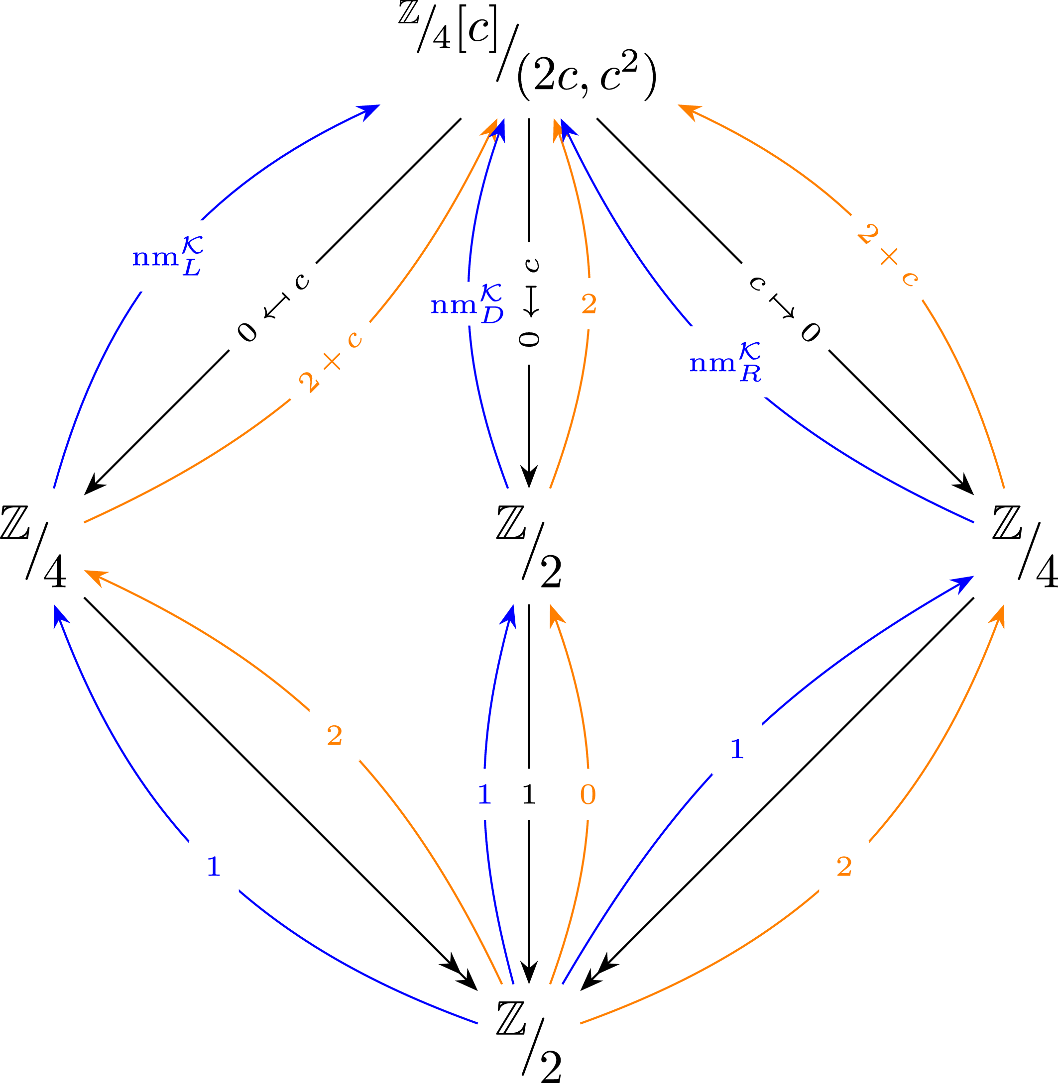
 K
K nDK(F2_)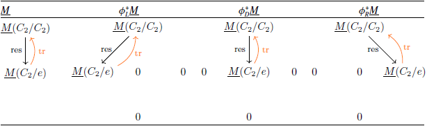
 ϕH∗:Mack(C2)→Mack(K)
 C2≅K/H
 ϕLDR∗M_:=ϕL∗M_⊕ϕD∗M_⊕ϕR∗M_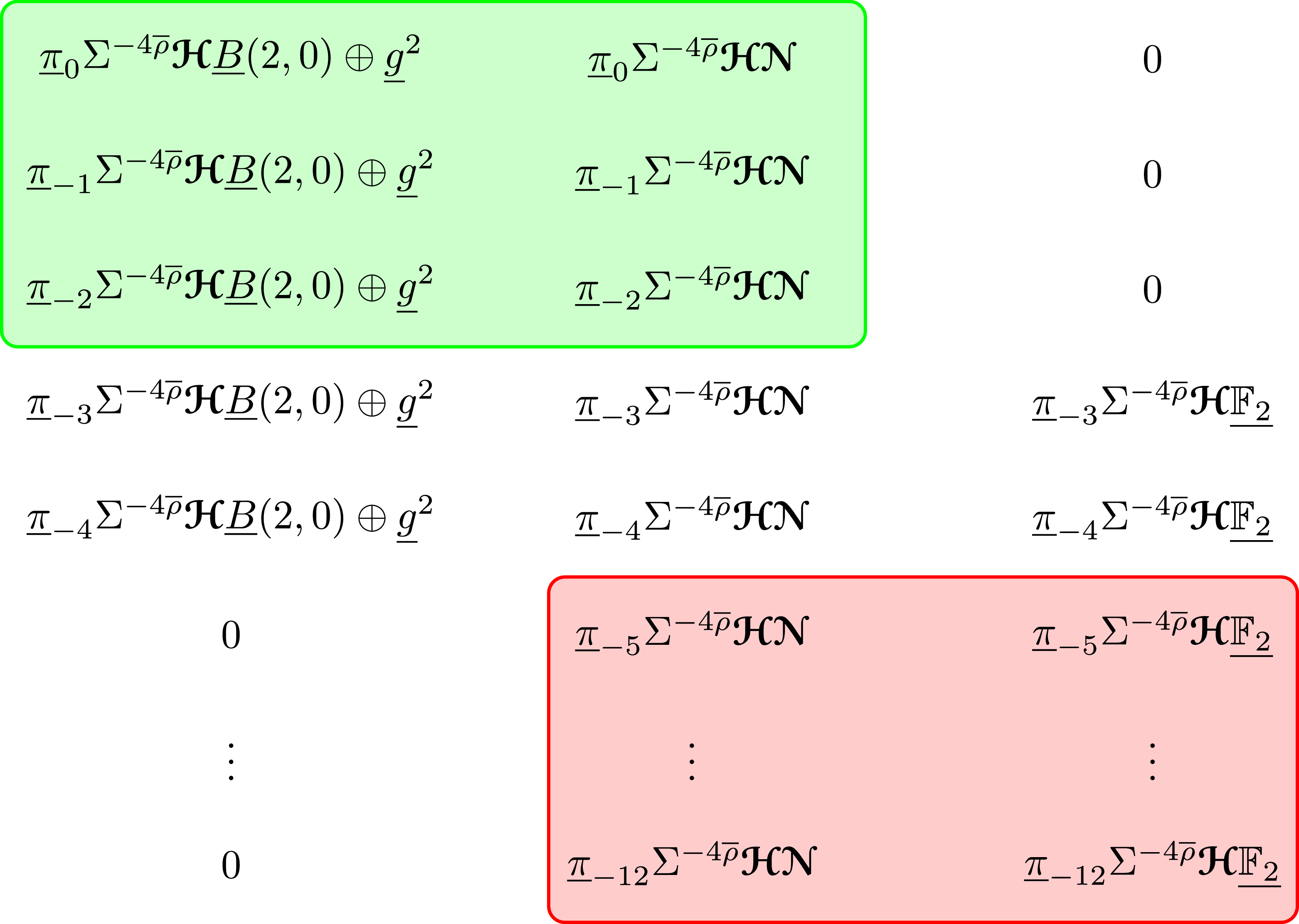
 π_∗Σ−4ρ¯HB_(2,0)⊕g_2→π_∗Σ−4ρ¯HN→π_∗Σ−4ρ¯HF2_
 Σ−4ρ¯HN
 HF2_
HF2_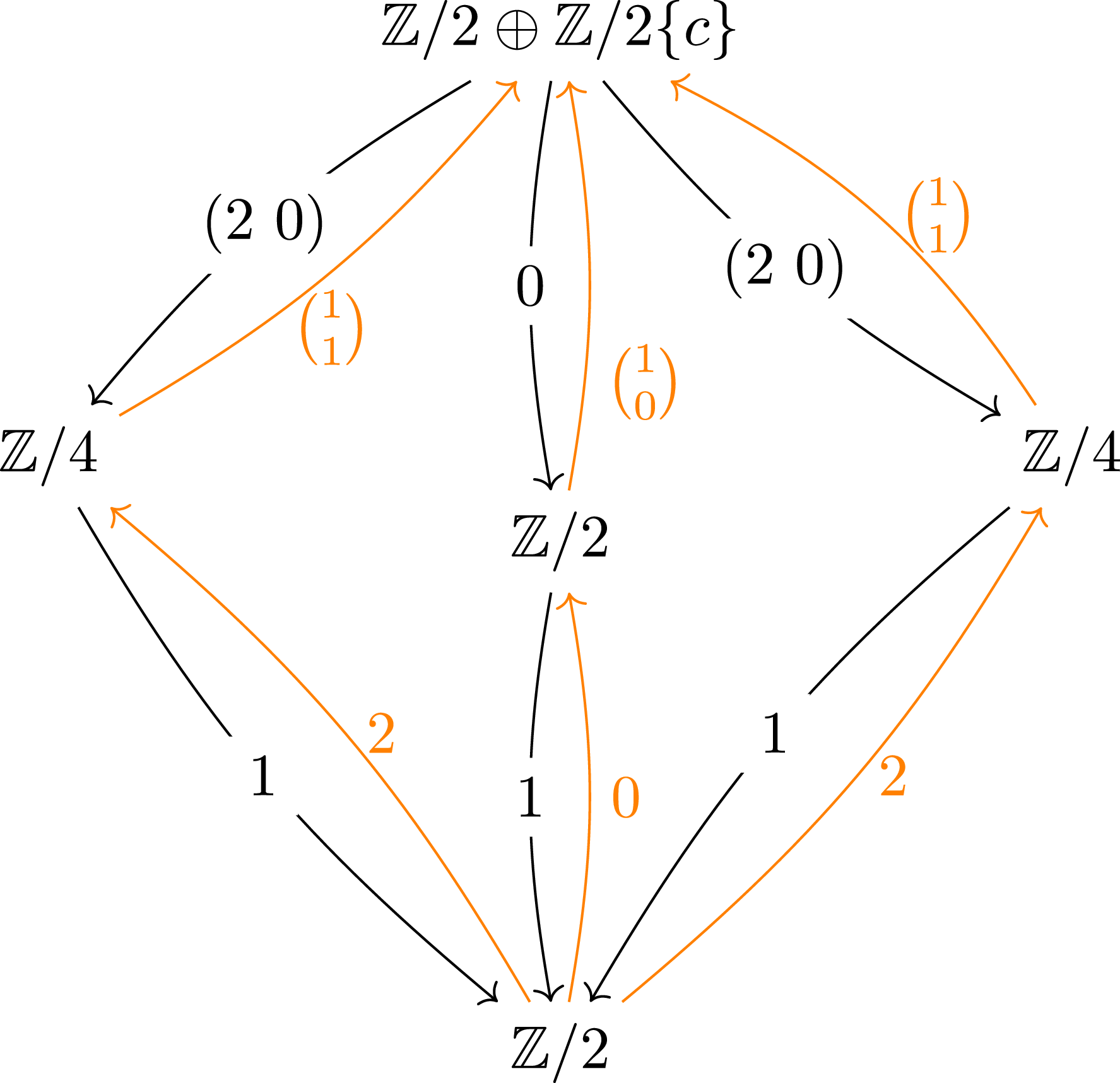
 K
K ND¯=NDKF2_¯
 NDK(F2_)→g_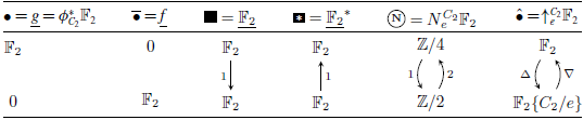
 C2
C2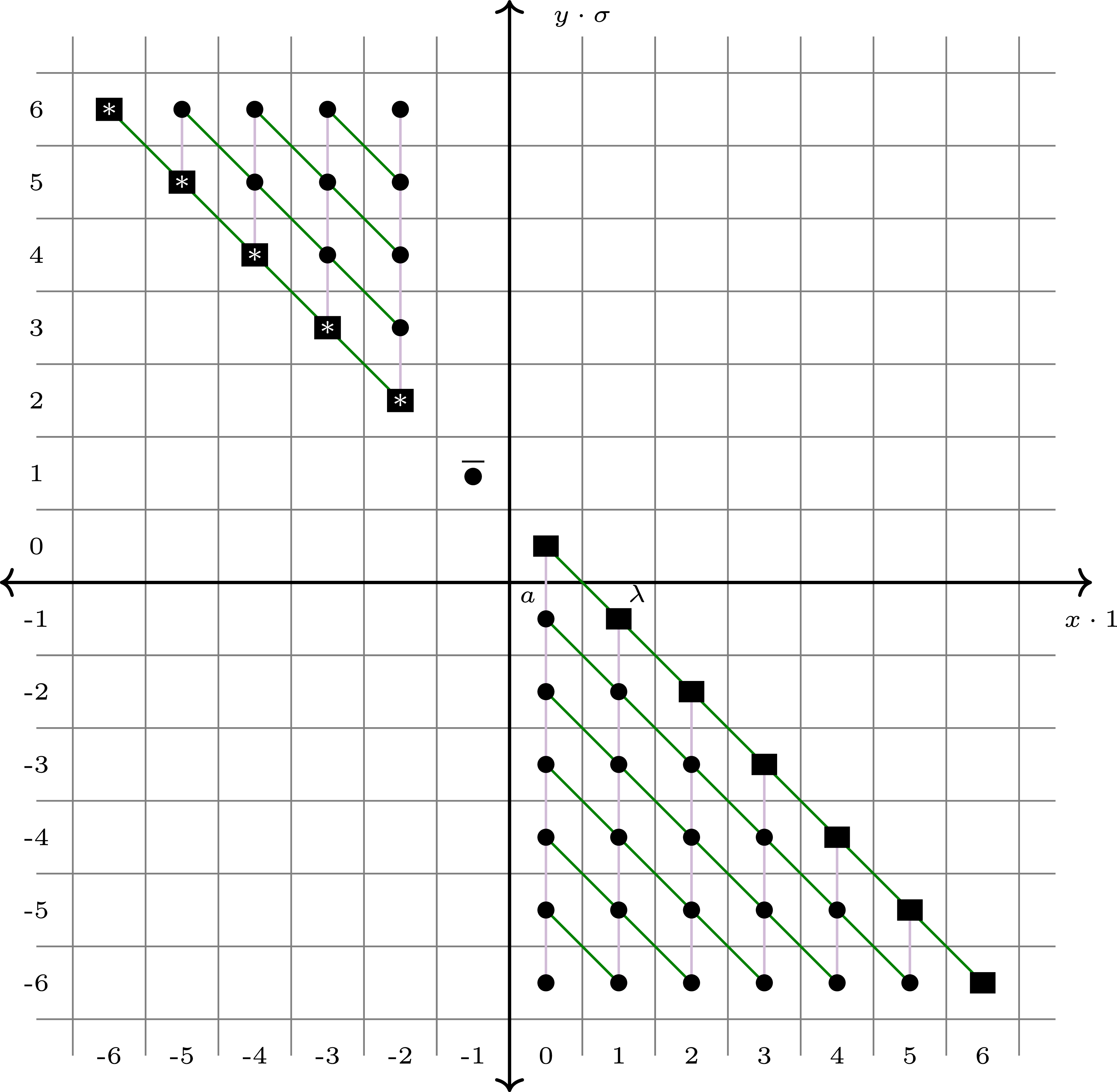
 π_x+yρ¯C2HF2_
 π_x+yρ¯C2HNeC2F2
 π_x+yρ¯C2NeC2HF2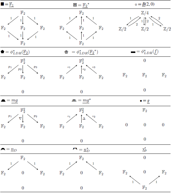
 K4
K4
 π_x+yρ¯KHF2_
 π_x+yρ¯KHF2_
 π_x+yρ¯KHNeKF2
 π_x+yρ¯KHNeKF2
 π_x+yρ¯KHNDKF2_
 π_x+yρ¯KHNDKF2
 Open access

