





1. Introduction
The F-signature is a fundamental numerical invariant of singularities in positive characteristic. Its positivity detects strong F-regularity, an important class of singularities related to KLT singularities in characteristic zero birational algebraic geometry. In this article, we compute the limiting F-signature function of binomial and other related hypersurfaces in two variables as the characteristic $p \to \infty $
.
$p \to \infty $
.
Fix a prime $p> 0$
and let
$p> 0$
and let $A_{p}$
denote either
$A_{p}$
denote either  the power series ring in n variables over the finite field $\mathbb {F}_{p}$
, or the local ring
$\mathbb {F}_{p}$
, or the local ring $\mathbb {F}_p [x_1, \ldots , x_n]_{(x_1, \ldots , x_n)}$
. Let
$\mathbb {F}_p [x_1, \ldots , x_n]_{(x_1, \ldots , x_n)}$
. Let $R = A_p / I$
for an ideal
$R = A_p / I$
for an ideal $I \subseteq A_p$
. It is natural to study the singularities of R using the behavior of the Frobenius or pth power endomorphism. By the work of Kunz [Reference Kunz17], R is regular if and only if Frobenius is flat, and in general, there are a number of numerical invariants of singularities which aim to measure the failure of flatness for the iterated Frobenius. Central among these are the Hilbert–Kunz multiplicity
$I \subseteq A_p$
. It is natural to study the singularities of R using the behavior of the Frobenius or pth power endomorphism. By the work of Kunz [Reference Kunz17], R is regular if and only if Frobenius is flat, and in general, there are a number of numerical invariants of singularities which aim to measure the failure of flatness for the iterated Frobenius. Central among these are the Hilbert–Kunz multiplicity $e_{\mathrm {HK}}(R)$
[Reference Monsky27] and F-signature
$e_{\mathrm {HK}}(R)$
[Reference Monsky27] and F-signature $s(R)$
[Reference Huneke and Leuschke16], [Reference Smith and Van den Bergh35], [Reference Tucker39], which can be expressed as
$s(R)$
[Reference Huneke and Leuschke16], [Reference Smith and Van den Bergh35], [Reference Tucker39], which can be expressed as
 $$ \begin{align*} e_{\mathrm{HK}}(R) = \lim_{e \to \infty} \frac{\min \left\{ m \mid \exists R^{\oplus m} \twoheadrightarrow F^e_*R \right\}}{p^{e\dim(R)}} \quad \text{and} \quad s(R) = \lim_{e \to \infty} \frac{\max \left\{ m \mid \exists F^e_*R \twoheadrightarrow R^{\oplus m} \right\}}{p^{e\dim(R)}}. \end{align*} $$
Provided R is equidimensional, both $e_{\mathrm {HK}}(R)$
and
$e_{\mathrm {HK}}(R)$
and $s(R)$
are
$s(R)$
are $1$
if and only if R is regular, and
$1$
if and only if R is regular, and $s(R)> 0$
if and only if R is strongly F-regular [Reference Aberbach and Leuschke1], [Reference Huneke and Leuschke16], [Reference Watanabe and Yoshida40]. On the other hand, these invariants are typically very hard to compute and the precise value is known only for certain limited classes of rings.
$s(R)> 0$
if and only if R is strongly F-regular [Reference Aberbach and Leuschke1], [Reference Huneke and Leuschke16], [Reference Watanabe and Yoshida40]. On the other hand, these invariants are typically very hard to compute and the precise value is known only for certain limited classes of rings.
In birational algebraic geometry, it is crucial to consider the singularities of divisor pairs. The notion of F-signature has been extended to the setting of divisor pairs in [Reference Blickle, Schwede and Tucker6], [Reference Blickle, Schwede and Tucker7], where the positivity of the F-signature again characterizes strong F-regularity. In the case of a hypersurface pair $(A_p, f^{t})$
, where
$(A_p, f^{t})$
, where $t \in \mathbb {R}_{\geq 0}$
and
$t \in \mathbb {R}_{\geq 0}$
and $f \in A_{p}$
is contained in
$f \in A_{p}$
is contained in $\mathfrak {m} = (x_1, \ldots , x_n)$
, we have
$\mathfrak {m} = (x_1, \ldots , x_n)$
, we have
 $$ \begin{align*} s(A_p, f^{t}) &= \lim_{e \to \infty} \frac{1}{p^{en}} \ell \left( \frac{A_p}{(x^{p^e}_{1}, \ldots, x^{p^e}_{n}):f^{\lceil tp^e \rceil}} \right) \\ &= 1 - \lim_{e \to \infty} \frac{1}{p^{en}} \ell \left( \frac{A_p}{(x^{p^e}_{1}, \ldots, x^{p^e}_{n},f^{\lceil tp^e \rceil})} \right). \end{align*} $$
While this non-increasing function is continuous [Reference Blickle, Schwede and Tucker7, Theorem 3.3] and even convex [Reference Blickle, Schwede and Tucker7, Theorem 3.9], one cannot expect the derivative of this function to behave well (see [Reference Blickle, Schwede and Tucker7, Remark 4.11] for such an example). More generally, when $n =\dim (R)= 2$
, the function
$n =\dim (R)= 2$
, the function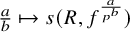 $\frac {a}{b} \mapsto s(R,f^{\frac {a}{p^b}})$
is a p-fractal in the sense of [Reference Monsky and Teixeira28], [Reference Monsky and Teixeira29] (see [Reference Blickle, Schwede and Tucker7, Section 4]).
$\frac {a}{b} \mapsto s(R,f^{\frac {a}{p^b}})$
is a p-fractal in the sense of [Reference Monsky and Teixeira28], [Reference Monsky and Teixeira29] (see [Reference Blickle, Schwede and Tucker7, Section 4]).
The F-signature function also encodes a number of important invariants of the hypersurface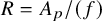 $R = A_p / (f)$
, namely, we have that
$R = A_p / (f)$
, namely, we have that
 $$\begin{align*}\partial_+ s(A_p, f^{0}) = - e_{HK}(R), \qquad \partial_- s(A_p, f^{1}) = - s(R), \end{align*}$$
and moreover the least t-intercept of $s(A_p, f^{t})$
is the F-pure threshold of the pair
$s(A_p, f^{t})$
is the F-pure threshold of the pair $(A_p,f)$
.
$(A_p,f)$
.
While the F-signature in a fixed characteristic p is not fully understood, it is hoped that limiting as the characteristic $p \to \infty $
might produce a more tractable invariant with additional geometric meaning. However, other than for diagonal hypersurfaces, few cases have been computed (see [Reference Caminata, Shideler, Tucker and Zerman9]). In this article, we add another class of examples in two variables. Our examples include binomials, and geometrically they encompass both three points in
$p \to \infty $
might produce a more tractable invariant with additional geometric meaning. However, other than for diagonal hypersurfaces, few cases have been computed (see [Reference Caminata, Shideler, Tucker and Zerman9]). In this article, we add another class of examples in two variables. Our examples include binomials, and geometrically they encompass both three points in $\mathbb P^1$
and the complete ADE (or simple) plane curve singularities (see [Reference Leuschke and Wiegand18, Section 4.3]).
$\mathbb P^1$
and the complete ADE (or simple) plane curve singularities (see [Reference Leuschke and Wiegand18, Section 4.3]).
Theorem A (Theorem 6.6, cf. [Reference Han13, Section 2])
Let $g = x^a y^b (x^u + y^v) ^c $
for non-negative integers
$g = x^a y^b (x^u + y^v) ^c $
for non-negative integers $a,b,c,u$
, and v. Assume that u, v, and c are positive. We consider g as a polynomial in
$a,b,c,u$
, and v. Assume that u, v, and c are positive. We consider g as a polynomial in $\mathbb {Z}[x,y]$
, so that we may consider the reduction of g to characteristic
$\mathbb {Z}[x,y]$
, so that we may consider the reduction of g to characteristic $p>0$
for each prime p. Set
$p>0$
for each prime p. Set $\lambda _0 = \frac {\frac {1}{u} + \frac {1}{v}}{\frac {a}{u} + \frac {b}{v} + c}$
, and
$\lambda _0 = \frac {\frac {1}{u} + \frac {1}{v}}{\frac {a}{u} + \frac {b}{v} + c}$
, and $\lambda = \min \{\frac {1}{a}, \frac {1}{b}, \frac {1}{c}, \lambda _0 \}$
. Let
$\lambda = \min \{\frac {1}{a}, \frac {1}{b}, \frac {1}{c}, \lambda _0 \}$
. Let $\psi (t)$
be the limit F-signature function of g, which is defined by
$\psi (t)$
be the limit F-signature function of g, which is defined by

Then, for $t < \lambda $
,
$t < \lambda $
, $\psi (t)$
is given by the following formula:
$\psi (t)$
is given by the following formula:
-
1. If $tav +u \geq tbu+v+cuvt$
, then
$\psi (t) = ( 1 -at) (1- (b +cv)t)$
.
$tav +u \geq tbu+v+cuvt$
, then
$\psi (t) = ( 1 -at) (1- (b +cv)t)$
. -
2. If
$tbu +v \geq tav+u+cuvt$
, then
$\psi (t) = (1-bt) (1 - (a +cu)t)$
. -
3. If
$tcuv + u + v \geq tav + tbu +2uv $
, then
$\psi (t) = (1-ct) (v(1-at) + u (1-bt) -uv)$
. -
4. Otherwise,
$\psi (t) = \frac {1}{4uv} (u+v - t(av + bu+ cuv))^2$
.







In fact, our methods are more precise and give an explicit computation of  for any p and $t \in \frac {1}{p} \mathbb {Z}_{\geq 0}$
when
$t \in \frac {1}{p} \mathbb {Z}_{\geq 0}$
when $u=v=1$
, see Theorem 6.4. This is achieved by giving an explicit Gröbner basis for ideals of the form
$u=v=1$
, see Theorem 6.4. This is achieved by giving an explicit Gröbner basis for ideals of the form $I= ( x^M, y^N, f^K)$
with
$I= ( x^M, y^N, f^K)$
with $f=x^ay^b(x+y)^c$
, for
$f=x^ay^b(x+y)^c$
, for $M,N,K,a,b,c$
all non-negative integers, and
$M,N,K,a,b,c$
all non-negative integers, and $M+(c-a)K \leq p$
(see Theorem 4.2).
$M+(c-a)K \leq p$
(see Theorem 4.2).
On the other hand, if one is solely interested in the length computations necessary for Theorem A, one can do a change of basis and analyze the Artinian Gorenstein algebra $\mathbb {F}_p[x,y,z]/(x^m, y^n, z^k)$
. In particular, we make use of the fact that for the values of
$\mathbb {F}_p[x,y,z]/(x^m, y^n, z^k)$
. In particular, we make use of the fact that for the values of $p,m,n$
, and k in our range of interest, this algebra has the weak Lefschetz property (WLP) [Reference Lundqvist and Nicklasson23]. We present this as an alternative computation to the explicit Gröbner computations in Section 5. Related computations of these lengths assuming some Lefschetz-type properties have previously been carried out in [Reference Han13, Section 2].
$p,m,n$
, and k in our range of interest, this algebra has the weak Lefschetz property (WLP) [Reference Lundqvist and Nicklasson23]. We present this as an alternative computation to the explicit Gröbner computations in Section 5. Related computations of these lengths assuming some Lefschetz-type properties have previously been carried out in [Reference Han13, Section 2].
An interesting consequence of the formulas obtained in Theorem 6.6 is that the values match with that of the normalized volume of the corresponding KLT pair computed by Li in [Reference Li20].
Corollary B (Theorem 7.2)
Let $(X, \Delta ) = (\operatorname {\mathrm {{Spec}}}(\mathbb {Z}[x,y]), \operatorname {\mathrm {div}} (f^t))$
, where
$(X, \Delta ) = (\operatorname {\mathrm {{Spec}}}(\mathbb {Z}[x,y]), \operatorname {\mathrm {div}} (f^t))$
, where $f= x^a \, y^b \, (x+y) ^c$
and
$f= x^a \, y^b \, (x+y) ^c$
and $t \geq 0$
is a rational parameter. Then, we have
$t \geq 0$
is a rational parameter. Then, we have
 $$\begin{align*}\frac{{\widehat{\rm vol}}(X_{\mathbb{C}}, \Delta_{\mathbb{C}})}{4} = \lim_{p \to \infty} s (X_p, \Delta_p), \end{align*}$$
where $X_{\mathbb {C}}$
and
$X_{\mathbb {C}}$
and $X_p$
denote the base changes of X to
$X_p$
denote the base changes of X to $\mathbb {C}$
and to
$\mathbb {C}$
and to $\mathbb {F}_p$
and localized at
$\mathbb {F}_p$
and localized at $(x,y)$
, respectively (and similarly for
$(x,y)$
, respectively (and similarly for $\Delta $
).
$\Delta $
).
The normalized volume introduced by Li [Reference Li19] is an invariant of singularities over the complex numbers detecting the stability properties of KLT singularities. While defined very differently, the normalized volume and the F-signature satisfy many analogous properties (see [Reference Carvajal-Rojas, Schwede and Tucker11], [Reference Ma, Polstra, Schwede and Tucker24], [Reference Taylor38]) and are expected to be closely related by reduction modulo p. While the exact nature of their relation is not clear, Theorem 7.2 provides further evidence toward their connection.
2. Preliminaries
In this section, we recall a number of numerical Frobenius invariants of singularities. See [Reference Blickle, Schwede and Tucker6] for the general definition of the F-signature functions in the pair and triples settings (especially Theorem 3.5); in this article, the following description in the hypersurface setting will suffice.
Definition 2.1 (F-signature function of hypersurface pairs)
[Reference Blickle, Schwede and Tucker6], [Reference Blickle, Schwede and Tucker7] Let $\mathbb {K}$
be a perfect field of characteristic
$\mathbb {K}$
be a perfect field of characteristic $p> 0$
,
$p> 0$
,  or the local ring $\mathbb {K} [x_1, \ldots , x_n]_{(x_1, \ldots , x_n)}$
, and
$\mathbb {K} [x_1, \ldots , x_n]_{(x_1, \ldots , x_n)}$
, and $f \in \mathfrak {m} = (x_1, \ldots , x_n)$
non-zero. For
$f \in \mathfrak {m} = (x_1, \ldots , x_n)$
non-zero. For $t \in \mathbb {R}_{\geq 0}$
, the F-signature of the pair
$t \in \mathbb {R}_{\geq 0}$
, the F-signature of the pair $(R,f^t)$
is given by
$(R,f^t)$
is given by
 $$ \begin{align*} s(R, f^{t}) &= \lim_{e \to \infty} \frac{1}{p^{en}}\, \ell \left( \frac{R}{(x^{p^e}_{1}, \ldots, x^{p^e}_{n}):f^{\lceil tp^e \rceil}} \right) \\ &= 1 - \lim_{e \to \infty} \frac{1}{p^{en}}\, \ell \left( \frac{R}{(x^{p^e}_{1}, \ldots, x^{p^e}_{n},f^{\lceil tp^e \rceil})} \right). \end{align*} $$
By inspection, it is easy to see that $s(R,f^t)$
is non-increasing in
$s(R,f^t)$
is non-increasing in $t \in \mathbb {R}_{> 0}$
, and we have that
$t \in \mathbb {R}_{> 0}$
, and we have that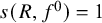 $s(R,f^0) = 1$
and
$s(R,f^0) = 1$
and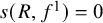 $s(R,f^1) = 0$
. In practice, computing
$s(R,f^1) = 0$
. In practice, computing $s(R,f^t)$
for arbitrary values of
$s(R,f^t)$
for arbitrary values of $t \in \mathbb {R}_{\geq 0}$
is difficult. However, if
$t \in \mathbb {R}_{\geq 0}$
is difficult. However, if $t = \frac {a}{p^b}$
with
$t = \frac {a}{p^b}$
with $a,b \in \mathbb {Z}$
, exploiting the flatness of Frobenius on R gives that
$a,b \in \mathbb {Z}$
, exploiting the flatness of Frobenius on R gives that
 $$ \begin{align} s(R, f^{\frac{a}{p^b}}) = \frac{1}{p^{bn}} \ell \left( \frac{R}{(x^{p^e}_{1}, \ldots, x^{p^e}_{n}):f^{a}} \right) = 1 - \frac{1}{p^{bn}} \ell \left( \frac{R}{(x^{p^e}_{1}, \ldots, x^{p^e}_{n},f^{a})} \right). \end{align} $$
Importantly, one can show that the function $t \mapsto s(R,f^t)$
is continuous [Reference Blickle, Schwede and Tucker7, Theorem 3.3] and even convex [Reference Blickle, Schwede and Tucker7, Theorem 3.9].
$t \mapsto s(R,f^t)$
is continuous [Reference Blickle, Schwede and Tucker7, Theorem 3.3] and even convex [Reference Blickle, Schwede and Tucker7, Theorem 3.9].
A key result about the F-signature states that $s(R, f^t)$
is positive if and only if
$s(R, f^t)$
is positive if and only if $(R,f^t)$
is strongly F-regular [Reference Blickle, Schwede and Tucker6, Theorem 3.18] (cf. [Reference Aberbach and Leuschke1]). Further, the smallest t-intercept of the F-signature function
$(R,f^t)$
is strongly F-regular [Reference Blickle, Schwede and Tucker6, Theorem 3.18] (cf. [Reference Aberbach and Leuschke1]). Further, the smallest t-intercept of the F-signature function $t \mapsto s(R,f^t)$
is the F-pure threshold of f, defined below.
$t \mapsto s(R,f^t)$
is the F-pure threshold of f, defined below.
Definition 2.2 (F-pure threshold)
[Reference Takagi and Watanabe37] Let $\mathbb {K}$
be a perfect field of characteristic
$\mathbb {K}$
be a perfect field of characteristic $p> 0$
,
$p> 0$
,  or the local ring $\mathbb {K} [x_1, \ldots , x_n]_{(x_1, \ldots , x_n)}$
, and
$\mathbb {K} [x_1, \ldots , x_n]_{(x_1, \ldots , x_n)}$
, and $f \in \mathfrak {m} = (x_1, \ldots , x_n)$
non-zero. The F-pure threshold of f (at
$f \in \mathfrak {m} = (x_1, \ldots , x_n)$
non-zero. The F-pure threshold of f (at $\mathfrak {m}$
) is
$\mathfrak {m}$
) is
 $$\begin{align*}\operatorname{\mathrm{{fpt}}}(f) = \sup \left\{ c = \frac{a}{p^e} \in {\mathbb{Z}}\left[\frac{1}{p}\right] \,\Big|\, f^a \not\in \mathfrak{m}^{[p^e]}\right\}. \end{align*}$$
While not immediate from the definition, the F-pure threshold is indeed a rational number [Reference Blickle, Mustaţǎ and Smith3]–[Reference Blickle, Schwede, Takagi and Zhang5]. It is closely related to another fundamental invariant, the log canonical threshold or $\operatorname {\mathrm {lct}}$
, whose origins lie in characteristic zero, where it can be computed using a resolution of singularities. See [Reference Benito, Faber and Smith2] for an elementary introduction to these invariants and the relationship between them. Here, we point out several of these connections in the context of reduction to characteristic
$\operatorname {\mathrm {lct}}$
, whose origins lie in characteristic zero, where it can be computed using a resolution of singularities. See [Reference Benito, Faber and Smith2] for an elementary introduction to these invariants and the relationship between them. Here, we point out several of these connections in the context of reduction to characteristic $p>0$
for future use.
$p>0$
for future use.
Proposition 2.3 [Reference Mustaţǎ, Takagi and Watanabe30, Theorems 3.3 and 3.4]
Let $f\in R=\mathbb Z[x_1,\ldots , x_n]$
be a non-zero polynomial contained in
$f\in R=\mathbb Z[x_1,\ldots , x_n]$
be a non-zero polynomial contained in $\mathfrak m=(x_1,\ldots , x_n)$
, so that by abuse of notation, we can view
$\mathfrak m=(x_1,\ldots , x_n)$
, so that by abuse of notation, we can view $f\in \mathbb Z/p\mathbb Z[x_1,\ldots , x_n]_{\mathfrak {m}}$
or in
$f\in \mathbb Z/p\mathbb Z[x_1,\ldots , x_n]_{\mathfrak {m}}$
or in $\mathbb Q[x_1,\ldots , x_n]_{\mathfrak {m}}$
. Then, for all
$\mathbb Q[x_1,\ldots , x_n]_{\mathfrak {m}}$
. Then, for all $p\gg 0$
, we have
$p\gg 0$
, we have $\operatorname {\mathrm {{fpt}}}(f) \leq \operatorname {\mathrm {lct}}(f)$
. Further,
$\operatorname {\mathrm {{fpt}}}(f) \leq \operatorname {\mathrm {lct}}(f)$
. Further, $\displaystyle \lim _{p\to \infty }\operatorname {\mathrm {{fpt}}}(f) = \operatorname {\mathrm {lct}}(f)$
.
$\displaystyle \lim _{p\to \infty }\operatorname {\mathrm {{fpt}}}(f) = \operatorname {\mathrm {lct}}(f)$
.
Definition 2.4 (Limit F-signature function)
Let $f \in R = {\mathbb {Z}}[x_1, \ldots , x_n]$
be a non-zero polynomial contained in
$f \in R = {\mathbb {Z}}[x_1, \ldots , x_n]$
be a non-zero polynomial contained in $\mathfrak {m} = (x_1, \ldots , x_n)$
. Note that for every prime
$\mathfrak {m} = (x_1, \ldots , x_n)$
. Note that for every prime $p>0$
such that
$p>0$
such that $f \notin pR$
, we can consider
$f \notin pR$
, we can consider $f_p \in {\mathbb {Z}}/p {\mathbb {Z}}[x_1, \ldots , x_n],$
which is a non-zero polynomial over
$f_p \in {\mathbb {Z}}/p {\mathbb {Z}}[x_1, \ldots , x_n],$
which is a non-zero polynomial over $\mathbb {F} _p$
. Thus, we can consider the functions
$\mathbb {F} _p$
. Thus, we can consider the functions $\psi _p (t)$
, defined as the F-signature of the pair
$\psi _p (t)$
, defined as the F-signature of the pair $(\mathbb {F}_p[x_1, \ldots , x_n]_{\mathfrak {m}}, f_p ^t)$
, as a sequence of functions defined for all
$(\mathbb {F}_p[x_1, \ldots , x_n]_{\mathfrak {m}}, f_p ^t)$
, as a sequence of functions defined for all $p \gg 0$
. We define the limit F-signature function
$p \gg 0$
. We define the limit F-signature function $\psi (t)$
as
$\psi (t)$
as
 $$\begin{align*}\psi(t) = \lim_{p \to \infty} \psi_p (t), \end{align*}$$
if it exists.
We note that the limit F-signature function is not known to exist outside of some special cases as in [Reference Caminata, Shideler, Tucker and Zerman9], [Reference Canton10]. However, as the following lemma shows, we do not need to compute the F-signature in every characteristic to compute the limit F-signature of polynomials over ${\mathbb {Z}}$
.
${\mathbb {Z}}$
.
Lemma 2.5. Let $f \in R = {\mathbb {Z}}[x_1, \ldots , x_n]$
be a non-zero polynomial contained in
$f \in R = {\mathbb {Z}}[x_1, \ldots , x_n]$
be a non-zero polynomial contained in $\mathfrak {m} = (x_1, \ldots , x_n)$
. For every prime p such that
$\mathfrak {m} = (x_1, \ldots , x_n)$
. For every prime p such that $f \notin pR$
, let
$f \notin pR$
, let $\psi _p (t)$
denote the F-signature of the pair
$\psi _p (t)$
denote the F-signature of the pair $(\mathbb {F}_p[x_1, \ldots , x_n]_{\mathfrak {m}}, f^t)$
. Suppose we have a continuous, non-increasing function
$(\mathbb {F}_p[x_1, \ldots , x_n]_{\mathfrak {m}}, f^t)$
. Suppose we have a continuous, non-increasing function $\psi (t)$
on the interval
$\psi (t)$
on the interval $[0,1]$
with
$[0,1]$
with $\psi (0) = 1$
and
$\psi (0) = 1$
and $\psi (1) = 0$
such that for each rational number
$\psi (1) = 0$
such that for each rational number $u \geq 0$
, there is sequence
$u \geq 0$
, there is sequence $r_p (u)$
of non-negative real numbers such that:
$r_p (u)$
of non-negative real numbers such that:
-
•
$r_p (u) \leq u$
for each
$p \gg 0$
and
$r_p (u) \to u$
as
$p \to \infty $
, and -
•
$\psi _p (r_p (u))$
converges to
$\psi (u)$
as
$p \to \infty $
.


Then, the sequence of functions $\psi _p$
converges uniformly to the function
$\psi _p$
converges uniformly to the function $\psi $
as
$\psi $
as $p \to \infty $
. In particular, if
$p \to \infty $
. In particular, if $\psi _p (u) \to \psi (u) $
as
$\psi _p (u) \to \psi (u) $
as $p \to \infty $
for each rational number u, then
$p \to \infty $
for each rational number u, then $\psi _p \to \psi $
uniformly.
$\psi _p \to \psi $
uniformly.
Proof. First, we show point-wise convergence: for each $t \in [0,1]$
, the sequence
$t \in [0,1]$
, the sequence $\psi _p (t)$
converges to
$\psi _p (t)$
converges to $\psi (t)$
. This is clear for
$\psi (t)$
. This is clear for $t = 0,1$
, so we assume that
$t = 0,1$
, so we assume that $ t$
is any real number in
$ t$
is any real number in $(0,1)$
. Choose
$(0,1)$
. Choose $u_1, u_2 \in (0,1) \cap \mathbb {Q}$
such that
$u_1, u_2 \in (0,1) \cap \mathbb {Q}$
such that $u_1 < t < u_2$
. Using our assumption, we know that the sequences
$u_1 < t < u_2$
. Using our assumption, we know that the sequences $\psi _p \left (r_p (u_1)\right )$
and
$\psi _p \left (r_p (u_1)\right )$
and $\psi _p \left (r_p(u_2)\right )$
converge to
$\psi _p \left (r_p(u_2)\right )$
converge to $\psi (u_1)$
and
$\psi (u_1)$
and $\psi (u_2),$
respectively (as
$\psi (u_2),$
respectively (as $p \to \infty $
). Since each function
$p \to \infty $
). Since each function $\psi _p$
is non-increasing, for each
$\psi _p$
is non-increasing, for each $p \gg 0,$
we have
$p \gg 0,$
we have
 $$\begin{align*}\psi_p\left(r_p(u_2)\right) \leq \psi_p (t) \leq \psi_p \left(r_p (u_1)\right). \end{align*}$$
This holds since $u_2>t$
implies we have
$u_2>t$
implies we have $r_p (u_2)> t$
for
$r_p (u_2)> t$
for $p \gg 0$
. By considering the limit
$p \gg 0$
. By considering the limit $p \gg 0$
in the above inequality, we have
$p \gg 0$
in the above inequality, we have
 $$ \begin{align} \psi(u_2) \leq \liminf_{p \to \infty} \psi_p (t) \leq \limsup_{p \to \infty} \psi_p (t) \leq \psi(u_1). \end{align} $$
Furthermore, taking rational numbers $u_1 \to t$
and
$u_1 \to t$
and $u_2 \to t$
and using the continuity of
$u_2 \to t$
and using the continuity of $\psi (t)$
, we must have
$\psi (t)$
, we must have $\limsup \psi _p (t) = \liminf \psi _p(t) = \psi (t)$
. This shows point-wise convergence of
$\limsup \psi _p (t) = \liminf \psi _p(t) = \psi (t)$
. This shows point-wise convergence of $\psi _p$
to
$\psi _p$
to $\psi $
.
$\psi $
.
The uniform convergence follows from point-wise convergence since each $\psi _p (t)$
is continuous and convex (see [Reference Niculescu and Persson32, Corollary 1.3.8]).
$\psi _p (t)$
is continuous and convex (see [Reference Niculescu and Persson32, Corollary 1.3.8]).
3. Lengths and Gröbner bases when
$f=x+y$

We will start by doing these computations in a simplified setting where $f=x+y$
is a polynomial in
$f=x+y$
is a polynomial in $\mathbb {K}[x,y]$
for
$\mathbb {K}[x,y]$
for $\mathbb {K}$
a field. More specifically, our goal in this section is to find a Gröbner basis for the ideal
$\mathbb {K}$
a field. More specifically, our goal in this section is to find a Gröbner basis for the ideal
 $$\begin{align*}I_{k,m,n} =(x^m, y^n, (x+y)^k), \end{align*}$$
and then use this to find the length
 $$\begin{align*}\ell_{k,m,n} = \ell(\mathbb{K}[x,y]/I_{k,m,n}). \end{align*}$$
We fix a monomial order with $x>y$
. In the first section, we will do a detailed Gröbner basis computation when
$x>y$
. In the first section, we will do a detailed Gröbner basis computation when $m\leq k$
, and use this to find the lengths. Then, in Section 3.2, we will use the old Gröbner basis to find a new one when
$m\leq k$
, and use this to find the lengths. Then, in Section 3.2, we will use the old Gröbner basis to find a new one when $m>k$
. Finally, in Section 3.3, we will compute the lengths
$m>k$
. Finally, in Section 3.3, we will compute the lengths $\ell _{k,m,n}$
.
$\ell _{k,m,n}$
.
3.1. Case
$m \leq k$

Our goal is to find a Gröbner basis for the ideal $I_{k,m,n}$
when
$I_{k,m,n}$
when $m\leq k$
. Inspired by Buchberger’s algorithm, we first compute some
$m\leq k$
. Inspired by Buchberger’s algorithm, we first compute some $\mathcal S$
-pairs. We will then give a nicer description of the resulting polynomials in Theorem 3.2, and we will give a complete Gröbner basis using some of these polynomials in Theorem 3.4.
$\mathcal S$
-pairs. We will then give a nicer description of the resulting polynomials in Theorem 3.2, and we will give a complete Gröbner basis using some of these polynomials in Theorem 3.4.
We will write $T^x_m(g)$
to mean the “truncation of g at
$T^x_m(g)$
to mean the “truncation of g at $x^m$
,” that is, we throw away all terms whose x-degree is
$x^m$
,” that is, we throw away all terms whose x-degree is $\geq m$
. Similarly,
$\geq m$
. Similarly, $T^y_n(g)$
means throwing away all terms whose y-degree is
$T^y_n(g)$
means throwing away all terms whose y-degree is $\geq n$
.
$\geq n$
.
Definition 3.1. Define
 $$\begin{align*}f_1 &=T_m^x f^k= \sum_{j=0}^{m-1} \binom{k}{j} x^{j} y^{k-j}.\\f_2 &= x f_1 - \binom{k}{m-1} y^{k-m+1} x^m = \sum_{j=0}^{m-2} \binom{k}{j} x^{j+1}y^{k-j}.\end{align*}$$
Now for $t<m$
, recursively define
$t<m$
, recursively define
 $$ \begin{align*} \begin{array}{rcl} f_{2t+1} &=& \displaystyle yf_{2t-1} - \left(\displaystyle\frac{k+2t-m}{m-t}\right) f_{2t}.\\ f_{2t+2} &=& \left(\displaystyle \frac{k+2t-m+1}{k+t-m+1}\right) x f_{2t+1} - \left(\displaystyle\frac{t(k+t)}{(k+t-m+1)(m-t)}\right) y f_{2t}. \end{array} \end{align*} $$
We use the convention that the empty product is 1. The following proposition solves the recursion.
Proposition 3.2. The recursion for $0 \leq t <m$
(or
$0 \leq t <m$
(or $1\leq t < m$
for the even case) is solved by the following functions:
$1\leq t < m$
for the even case) is solved by the following functions:
 $$\begin{align*}\begin{array}{rcl} f_{2t+1} & =& \displaystyle \sum_{j=0}^{m-1-t} \frac{\prod_{\ell=1}^{t}(m-j-\ell)}{\prod_{\ell=1}^{t}(m-\ell)}\binom{k+t}{j}x^{j}y^{k-j+t}.\\ f_{2t} & = &\displaystyle \sum_{j=0}^{m-1-t} \frac{\prod_{\ell=2}^{t}(m-j-\ell)}{\prod_{\ell=1}^{t-1}(m-\ell)}\binom{k+t-1}{j} x^{j+1}y^{k-j+t-1}. \end{array} \end{align*}$$
Proof. When $t=0$
,
$t=0$
, $f_{2t+1}$
simplifies to
$f_{2t+1}$
simplifies to $f_1$
. Similarly, when
$f_1$
. Similarly, when $t=1$
,
$t=1$
, $f_{2t}$
simplifies to
$f_{2t}$
simplifies to $f_2$
. We now check the recursions. Substituting the expressions for
$f_2$
. We now check the recursions. Substituting the expressions for $f_{2t}$
and
$f_{2t}$
and $f_{2t+1}$
into the equation
$f_{2t+1}$
into the equation
 $$\begin{align*}f_{2t+2} = \frac{k+2t-m+1}{k+t-m+1}x f_{2t+1} - \frac{t(k+t)}{(k+t-m+1)(m-t)}y f_{2t}, \end{align*}$$
we see that
 $$ \begin{align*}\displaystyle f_{2t+2} &= \displaystyle \left(\frac{k+2t-m+1}{k+t-m+1}\right) x \left(\sum_{j=0}^{m-1-t} \frac{\prod_{\ell=1}^{t}(m-j-\ell)}{\prod_{\ell=1}^{t}(m-\ell)} \binom{k+t}{j} x^{j}y^{k-j+t}\right) \\ &\quad- \displaystyle \left(\frac{t(k+t)}{(k+t-m+1)(m-t)}\right) y \left(\sum_{j=0}^{m-1-t} \frac{\prod_{\ell=2}^{t}(m-j-\ell) }{ \prod_{\ell=1}^{t-1}(m-\ell)} \binom{k+t-1}{j} x^{j+1}y^{k-j+t-1}\right) \end{align*} $$
and so the coefficient of $x^{j+1} y^{k-j+t}$
is
$x^{j+1} y^{k-j+t}$
is
 $$ \begin{align*} &\left(\frac{k+2t-m+1}{k+t-m+1}\right) \left(\frac{\prod_{\ell=1}^{t}(m-j-\ell)}{\prod_{\ell=1}^{t}(m-\ell)}\right) \binom{k+t}{j} \\ &\qquad\qquad\qquad - \left(\frac{t(k+t)}{(k+t-m+1)(m-t)}\right) \left(\frac{\prod_{\ell=2}^{t}(m-j-\ell) }{ \prod_{\ell=1}^{t-1}(m-\ell)}\right) \binom{k+t-1}{j}. \end{align*} $$
Factoring out the common product of fractions and a binomial coefficient
 $$\begin{align*}\left(\frac{\prod_{\ell=2}^{t}(m-j-\ell)}{\prod_{\ell=1}^{t-1}(m-\ell)}\right) \binom{k+t-1}{j},\end{align*}$$
we are left with
 $$\begin{align*}\left(\frac{(k+2t-m+1)(m-j-1) }{ (k+t-m+1)(m-t)}\right) \left(\frac{k+t}{k+t-j}\right) - \left(\frac{t(k+t)}{(k+t-m+1)(m-t)}\right),\end{align*}$$
which simplifies to
 $$\begin{align*}\frac{(m-j-t-1)(k+t)}{(m-t) (k+t-j)}.\end{align*}$$
We can now recombine these extra factors into the binomial coefficient and the fraction of products out front to get an $x^{j+1}y^{k-j+t}$
coefficient of
$x^{j+1}y^{k-j+t}$
coefficient of
 $$\begin{align*}\left(\frac{\prod_{\ell=2}^{t+1}(m-j-\ell)}{\prod_{\ell=1}^{t}(m-\ell)}\right)\binom{k+t}{j}. \end{align*}$$
Thus,
 $$ \begin{align*} f_{2t+2} &= \sum_{j=0}^{m-1-t} \left(\frac{\prod_{\ell=2}^{t+1}(m-j-\ell)}{\prod_{\ell=1}^{t}(m-\ell)}\right) \binom{k+t}{j} x^{j+1}y^{k-j+t} \\ &=\sum_{j=0}^{m-2-t} \left(\frac{\prod_{\ell=2}^{t+1}(m-j-\ell)}{\prod_{\ell=1}^{t}(m-\ell)}\right) \binom{k+t}{j} x^{j+1}y^{k-j+t} , \end{align*} $$
since when $j=m-1-t$
, the
$j=m-1-t$
, the $\ell =t+1$
term of the product
$\ell =t+1$
term of the product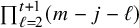 $\prod _{\ell =2}^{t+1}(m-j-\ell )$
is zero. Hence, the recursion is satisfied.
$\prod _{\ell =2}^{t+1}(m-j-\ell )$
is zero. Hence, the recursion is satisfied.
Similarly, substituting the expressions for $f_{2t-1}$
and
$f_{2t-1}$
and $f_{2t}$
into
$f_{2t}$
into
 $$\begin{align*}f_{2t+1} = y f_{2t-1} - \left(\frac{k+2t-m}{m-t}\right) f_{2t}, \end{align*}$$
we obtain that
 $$ \begin{align*} f_{2t+1}&= y \sum_{j=0}^{m-t} \frac{\prod_{\ell=1}^{t-1}(m-j-\ell)}{\prod_{\ell=1}^{t-1}(m-\ell)}\binom{k+t-1}{j}x^{j}y^{k-j+t-1} \\ & \quad- \left(\frac{k+2t-m}{m-t} \right) \sum_{j=0}^{m-1-t} \frac{\prod_{\ell=2}^{t}(m-j-\ell)}{\prod_{\ell=1}^{t-1}(m-\ell)} \binom{k+t-1}{j} x^{j+1}y^{k-j+t-1} \\ &= \sum_{j=0}^{m-t} \frac{\prod_{\ell=1}^{t-1}(m-j-\ell)}{\prod_{\ell=1}^{t-1}(m-\ell)}\binom{k+t-1}{j}x^{j}y^{k-j+t} \\& \quad- \left(\frac{k+2t-m}{m-t}\right) \sum_{j=1}^{m-t} \left( \frac{\prod_{\ell=1}^{t-1}(m-j-\ell)}{\prod_{\ell=1}^{t-1}(m-\ell)} \right) \binom{k+t-1}{j-1} x^{j}y^{k-j+t}. \end{align*} $$
When $j=0$
, the coefficient of
$j=0$
, the coefficient of $y^{k-t}$
is already of the form
$y^{k-t}$
is already of the form
 $$\begin{align*}\frac{\prod_{\ell=1}^{t-1}(m-\ell)}{\prod_{\ell=1}^{t-1}(m-\ell)}\binom{k+t-1}{0} = 1 = \frac{\prod_{\ell=1}^{t}(m-\ell)}{\prod_{\ell=1}^{t}(m-\ell)}\binom{k+t}{0}. \end{align*}$$
Otherwise, for $1\leq j \leq m-t$
, we have an
$1\leq j \leq m-t$
, we have an $x^j y^{k-j+t}$
coefficient of
$x^j y^{k-j+t}$
coefficient of
 $$ \begin{align*} &\left( \frac{\prod_{\ell=1}^{t-1}(m-j-\ell)}{\prod_{\ell=1}^{t-1}(m-\ell)}\right) \binom{k+t-1}{j} - \left(\frac{k+2t-m}{m-t}\right)\left( \frac{\prod_{\ell=1}^{t-1}(m-j-\ell)}{\prod_{\ell=1}^{t-1}(m-\ell)} \right) \binom{k+t-1}{j-1}\\ &\quad =\left(\frac{\prod_{\ell=1}^{t-1}(m-j-\ell)}{\prod_{\ell=1}^{t}(m-\ell)}\right) \left( \frac{(k+t-1)!}{j!(k+t-j)!} \right) \Big((k+t-j)(m-t)- j(k+2t-m)\Big). \end{align*} $$
Since $(k+t-j)(m-t)- j(k+2t-m) = (k+t)(m-j-t)$
and since the coefficient again simplifies to zero when
$(k+t-j)(m-t)- j(k+2t-m) = (k+t)(m-j-t)$
and since the coefficient again simplifies to zero when $j=m-t$
, we obtain that
$j=m-t$
, we obtain that
 $$\begin{align*}f_{2t+1} = \sum_{j=0}^{m-t-1} \frac{\prod_{\ell=1}^{t}(m-j-\ell)}{\prod_{\ell=1}^{t}(m-\ell)} \binom{k+t}{j} x^{j}y^{k-j+t}. \end{align*}$$
This concludes the induction.
Now, we have the following useful lemma.
Lemma 3.3. Let $m\leq k$
and
$m\leq k$
and $m+k\leq p$
for a prime number p, and let
$m+k\leq p$
for a prime number p, and let $1 \leq s < 2m$
be an integer. Let
$1 \leq s < 2m$
be an integer. Let $f_s$
be one of the functions recursively defined in Definition 3.1. Then, p does not divide any of the coefficients of
$f_s$
be one of the functions recursively defined in Definition 3.1. Then, p does not divide any of the coefficients of $f_s$
.
$f_s$
.
In particular, in both characteristic zero and characteristic p, the $f_{s}$
polynomials have leading terms
$f_{s}$
polynomials have leading terms
 $$ \begin{align*} \operatorname{\mathrm{in}}(f_{2t+1}) &= \frac{\prod_{\ell=1}^{t}(t-\ell+1)}{\prod_{\ell=1}^{t}(m-\ell)}\binom{k+t}{m-t-1}x^{m-t-1}y^{k-m+2t+1} = \frac{\binom{k+t}{m-t-1}}{\binom{m-1}{t}} x^{m-1-t}y^{k+2t+1 - m}, \\ \operatorname{\mathrm{in}}(f_{2t}) &= \frac{\prod_{\ell=2}^{t} (t-\ell+1)}{\prod_{\ell=1}^{t-1}(m-\ell)} \binom{k+t-1}{m-t-1}x^{m-t}y^{k-m+2t} = \frac{\binom{k+t-1}{m-t-1}}{\binom{m-1}{t-1}} x^{m-t} y^{k+2t -m}. \end{align*} $$
Proof. Write either $s=2t$
or
$s=2t$
or $s=2t+1$
, depending on parity. We may assume
$s=2t+1$
, depending on parity. We may assume $s\geq 3$
(and thus
$s\geq 3$
(and thus $m,t\geq 1$
) since the result clearly holds in the base cases. Recall that the recursion coefficients appearing in Theorem 3.1 are
$m,t\geq 1$
) since the result clearly holds in the base cases. Recall that the recursion coefficients appearing in Theorem 3.1 are $\frac {k+2t-m}{m-t}$
,
$\frac {k+2t-m}{m-t}$
, $\frac {k+2t-m+1}{k+t-m+1}$
, and
$\frac {k+2t-m+1}{k+t-m+1}$
, and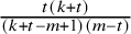 $\frac {t(k+t)}{(k+t-m+1)(m-t)}$
. Since
$\frac {t(k+t)}{(k+t-m+1)(m-t)}$
. Since $t<m\leq k$
and
$t<m\leq k$
and $1\leq t \leq k+t<k+m\leq p$
, we have that
$1\leq t \leq k+t<k+m\leq p$
, we have that
 $$ \begin{align*} 1\leq k+t-m+1 \leq k+2t-m+1 < k+t+1 \leq k+m \leq p \end{align*} $$
and similarly that $1\leq k+2t-m <p$
. Hence, all the coefficients appearing in the definitions of the recursion are nonzero and less than p. Therefore, the functions
$1\leq k+2t-m <p$
. Hence, all the coefficients appearing in the definitions of the recursion are nonzero and less than p. Therefore, the functions $f_s$
are well-defined in characteristic p.
$f_s$
are well-defined in characteristic p.
If $s=2t+1$
, then for
$s=2t+1$
, then for $0 \leq j \leq m-t-1$
, the
$0 \leq j \leq m-t-1$
, the $x^jy^{k-j+t}$
coefficient of
$x^jy^{k-j+t}$
coefficient of $f_s$
is
$f_s$
is
 $$\begin{align*}\frac{\prod_{\ell=1}^{t}(m-j-\ell)}{\prod_{\ell=1}^{t}(m-\ell)} \binom{k+t}{j}. \end{align*}$$
This coefficient is non-zero and well-defined since
 $$\begin{align*}1\leq m-j-t\leq m-t, \ \ 1\leq k+t,\ \textrm{ and } \ j\leq m-t-1<m\leq k<k+t. \end{align*}$$
This coefficient is not divisible by p because $m-j-\ell , m-\ell < m \leq p$
and
$m-j-\ell , m-\ell < m \leq p$
and $k+t<k+m<p$
.
$k+t<k+m<p$
.
If $s=2t$
, then since
$s=2t$
, then since $s\geq 3,$
we may in fact assume
$s\geq 3,$
we may in fact assume $t\geq 2$
. For
$t\geq 2$
. For $0 \leq j \leq m-t-1$
, the
$0 \leq j \leq m-t-1$
, the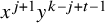 $x^{j+1}y^{k-j+t-1}$
coefficient of
$x^{j+1}y^{k-j+t-1}$
coefficient of $f_s$
is
$f_s$
is
 $$\begin{align*}\frac{\prod_{\ell=2}^{t}(m-j-\ell)}{\prod_{\ell=1}^{t-1}(m-\ell)}\binom{k+t-1}{j}. \end{align*}$$
This coefficient is non-zero and well-defined since
 $$\begin{align*}1\leq m-j-t\leq m-t+1,\ \ 1\leq k+t-1,\ \textrm{ and } \ j\leq m-t-1 <m\leq k+t-1. \end{align*}$$
This coefficient is not divisible by p because $m-\ell , m-j-\ell < m \leq p,$
and
$m-\ell , m-j-\ell < m \leq p,$
and $k+t-1 < k+m < p$
. This concludes the proof of the lemma.
$k+t-1 < k+m < p$
. This concludes the proof of the lemma.
Proposition 3.4. Assume that $m \leq k $
, that
$m \leq k $
, that $I_{k,m,n}=(x^m,y^n,(x+y)^k)$
, and that the
$I_{k,m,n}=(x^m,y^n,(x+y)^k)$
, and that the $f_{2t+1}$
are as in Theorem 3.2. Fix a monomial order with
$f_{2t+1}$
are as in Theorem 3.2. Fix a monomial order with $x>y$
.
$x>y$
.
-
1. If the field
$\mathbb {K}$
has characteristic
$0$
, then the elements
$$\begin{align*}x^m, y^n, f_{2t+1} \ \ \text{for} \ \ 0 \leq t < m\end{align*}$$
form a Gröbner basis of the ideal
$I_{k,m,n}$
. -
2. If the field
$\mathbb {K}$
has characteristic p and
$m+k\leq p$
, then the elements
$$\begin{align*}x^m, y^n, f_{2t+1} \ \ \text{for} \ \ 0 \leq t < m\end{align*}$$
form a Gröbner basis of the ideal
$I_{k,m,n}$
.


Remark 3.5. In fact, since $y^n$
is in the proposed Gröbner basis, this means that taking
$y^n$
is in the proposed Gröbner basis, this means that taking $x^m$
,
$x^m$
, $y^n$
,
$y^n$
, $T^y_nf_{2t+1}$
should also be a Gröbner basis. This truncation is non-zero whenever the smallest y-degree appearing in a term is
$T^y_nf_{2t+1}$
should also be a Gröbner basis. This truncation is non-zero whenever the smallest y-degree appearing in a term is $<n$
, that is, whenever
$<n$
, that is, whenever $2t+k+1-m <n$
or equivalently
$2t+k+1-m <n$
or equivalently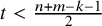 $t<\frac {n+m-k-1}{2}$
. Thus, a Gröbner basis is precisely the polynomials
$t<\frac {n+m-k-1}{2}$
. Thus, a Gröbner basis is precisely the polynomials
 $$\begin{align*}x^m, y^n, T^y_n f_{2t+1} \ \ \text{for}\ \ 0\leq t < \min\left(m, \frac{n+m-k-1}{2}\right). \end{align*}$$
Proof of Theorem 3.4
Given an element $g \in I_{k,m,n}$
, we will show that the leading term is divisible by
$g \in I_{k,m,n}$
, we will show that the leading term is divisible by $x^m$
,
$x^m$
, $y^n$
, or the leading term of one of the
$y^n$
, or the leading term of one of the $T_n^y f_{2t+1}$
. Any element of
$T_n^y f_{2t+1}$
. Any element of $I_{k,m,n}$
can be expressed as
$I_{k,m,n}$
can be expressed as
 $$\begin{align*}g = g_1 x^m + g_2 y^n + h f^k,\end{align*}$$
where $g_1, g_2, h \in \mathbb {K}[x,y]$
. If the leading term of g is divisible by
$g_1, g_2, h \in \mathbb {K}[x,y]$
. If the leading term of g is divisible by $x^m$
or
$x^m$
or $y^n$
, we are done. We may therefore assume that the leading term
$y^n$
, we are done. We may therefore assume that the leading term $x^{\alpha }y^{\beta }$
of g has
$x^{\alpha }y^{\beta }$
of g has $\alpha <m$
and
$\alpha <m$
and $\beta < n$
. Since every term in
$\beta < n$
. Since every term in $g_1 x^m + g_2 y^n$
is divisible by
$g_1 x^m + g_2 y^n$
is divisible by $x^m$
or
$x^m$
or $y^n$
, the term
$y^n$
, the term $x^{\alpha }y^{\beta }$
must be the leading term of
$x^{\alpha }y^{\beta }$
must be the leading term of $h f^k$
modulo the terms that are divisible by
$h f^k$
modulo the terms that are divisible by $x^m$
or
$x^m$
or $y^n$
.
$y^n$
.
Since the ideal $I_{k,m,n}$
is homogeneous with respect to the usual grading on
$I_{k,m,n}$
is homogeneous with respect to the usual grading on $\mathbb {K}[x,y]$
, it is sufficient to consider the case where
$\mathbb {K}[x,y]$
, it is sufficient to consider the case where $g_1$
,
$g_1$
, $g_2$
, and h are all homogeneous polynomials, and so we can write our non-zero h as
$g_2$
, and h are all homogeneous polynomials, and so we can write our non-zero h as $h(x,y) = \sum _{\ell = 0}^{d} a_\ell x^{\ell }y^{d - \ell }$
. We first compute
$h(x,y) = \sum _{\ell = 0}^{d} a_\ell x^{\ell }y^{d - \ell }$
. We first compute
 $$ \begin{align*} hf^k &= \left(\sum_{\ell = 0}^{d} a_\ell x^{\ell}y^{d-\ell}\right) \left(\sum_{j= 0} ^{k} \binom{k}{j} x^{j} y^{k-j}\right) \\ &= \sum_{j=0}^{k+d} \left( \sum_{\ell = \max(0, j-k)}^{\min(d,j)} a_\ell \binom{k}{j-\ell} \right) x^{j} y^{k+d-j}. \end{align*} $$
Note that we can express this information succinctly in a (labeled) matrix:

where the row labeled $"j"$
corresponds to the term where the x-degree equals j. The coefficient of the
$"j"$
corresponds to the term where the x-degree equals j. The coefficient of the $x^{j}$
term is the product of the j-row with the column vector
$x^{j}$
term is the product of the j-row with the column vector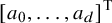 $\left [ a_0, \ldots , a_d \right ] ^{\text {T}}$
. Suppose the leading term of
$\left [ a_0, \ldots , a_d \right ] ^{\text {T}}$
. Suppose the leading term of $T^x_m (h f^k)$
is
$T^x_m (h f^k)$
is $x^{\alpha } y^{\beta }$
for non-negative integers
$x^{\alpha } y^{\beta }$
for non-negative integers $\alpha $
and
$\alpha $
and $\beta $
such that
$\beta $
such that $\alpha <m$
. Let
$\alpha <m$
. Let $t=m-1-\alpha $
, so that
$t=m-1-\alpha $
, so that
 $$\begin{align*}\alpha = m-1-t \end{align*}$$
and $0 \leq t < m $
. Note that by homogeneity,
$0 \leq t < m $
. Note that by homogeneity,
 $$\begin{align*}\beta = k+d - \alpha = k + d + t +1-m. \end{align*}$$
We will show that this choice of t ensures that this leading term $x^{\alpha } y^\beta $
is a multiple of
$x^{\alpha } y^\beta $
is a multiple of $\operatorname {\mathrm {in}}( f_{2t+1})$
. It suffices to show
$\operatorname {\mathrm {in}}( f_{2t+1})$
. It suffices to show $\beta \geq k+2t +1-m$
, so that
$\beta \geq k+2t +1-m$
, so that $x^{\alpha }y^{\beta }$
is divisible by
$x^{\alpha }y^{\beta }$
is divisible by $x^{m-1-t} y^{k+2t+1-m}$
(our assumed constraints and Theorem 3.3 ensure that this is indeed the correct initial monomial). If we knew that
$x^{m-1-t} y^{k+2t+1-m}$
(our assumed constraints and Theorem 3.3 ensure that this is indeed the correct initial monomial). If we knew that $d\geq t$
, then we would have
$d\geq t$
, then we would have
 $$\begin{align*}\beta = k + d +t+1-m \geq k + 2t + 1 - m\end{align*}$$
as desired. Thus, all that remains is to prove the following claim.
Claim. $d \geq t$
.
$d \geq t$
.
Proof of claim. We will obtain a contradiction by instead assuming $ d+1 \leq t$
. Consider the terms appearing in
$ d+1 \leq t$
. Consider the terms appearing in $T^x_m (h f^k)$
. By assumption, the coefficient of
$T^x_m (h f^k)$
. By assumption, the coefficient of $x^{\alpha } y^{\beta }$
is nonzero. Since this is the leading term, the coefficients of
$x^{\alpha } y^{\beta }$
is nonzero. Since this is the leading term, the coefficients of $x^{\alpha + \iota } y^{\beta - \iota }$
must vanish for
$x^{\alpha + \iota } y^{\beta - \iota }$
must vanish for $1 \leq \iota \leq t$
. By assumption, all the exponents appearing in this list are less than m. Consider these constraints on the coefficients of the
$1 \leq \iota \leq t$
. By assumption, all the exponents appearing in this list are less than m. Consider these constraints on the coefficients of the $x^{\alpha +\iota }y^{\beta -\iota }$
as a sequence of t equations with the
$x^{\alpha +\iota }y^{\beta -\iota }$
as a sequence of t equations with the $a_\ell $
as our unknowns. If
$a_\ell $
as our unknowns. If $t>d+k$
, we can simply consider the extra constraints as “trivial” constraints. Then, we make the following observations about the matrix representing this system of equations:
$t>d+k$
, we can simply consider the extra constraints as “trivial” constraints. Then, we make the following observations about the matrix representing this system of equations:
-
1. The “bottom” row corresponds to
$\iota = t$
, that is, the
$j = m-1$
row of
$M(f^k, m,n,d)$
. -
2. The “top” row corresponds to
$\iota =1$
, that is, the
$j = i - t+1=m -t$
row. -
3. The number of rows is equal to t, which is at least
$d+1$
by assumption.






Now, let D be the top $(d+1)\times (d+1)$
submatrix of these constraints, so that
$(d+1)\times (d+1)$
submatrix of these constraints, so that

or in other words, D is the matrix with entries
 $$\begin{align*}D_{i,j} = \binom{k}{m-t-i+j}\end{align*}$$
for $0\leq i,j\leq d$
. Then, by applying Theorem 3.6 to the matrix
$0\leq i,j\leq d$
. Then, by applying Theorem 3.6 to the matrix $D=D(k, m-t, d+t-m)$
, we see that D is always invertible in characteristic
$D=D(k, m-t, d+t-m)$
, we see that D is always invertible in characteristic $0$
, and is also invertible modulo p since
$0$
, and is also invertible modulo p since
 $$\begin{align*}k+(m-t)+(d+t-m) = k+d<k+t<k+(p-k)=p.\end{align*}$$
Thus, the only way for all of these coefficients of $x^{\alpha +\iota }y^{\beta -\iota }$
to be zero is for all of the
$x^{\alpha +\iota }y^{\beta -\iota }$
to be zero is for all of the $a_\ell $
to be zero. But this contradicts the fact that
$a_\ell $
to be zero. But this contradicts the fact that $h\neq 0$
, and thus
$h\neq 0$
, and thus $d\geq t$
, proving the claim.
$d\geq t$
, proving the claim.
Lemma 3.6. Let $k,a,v$
be three integers such that
$k,a,v$
be three integers such that $0 \leq a \leq k$
and
$0 \leq a \leq k$
and $a+v \geq 0$
. Let
$a+v \geq 0$
. Let $D(k,a,v)$
be the
$D(k,a,v)$
be the $(a+v+1) \times (a+v+1)$
matrix with entries
$(a+v+1) \times (a+v+1)$
matrix with entries $D(k, a, v)_{i,j} = \binom {k}{a-i+j}$
for
$D(k, a, v)_{i,j} = \binom {k}{a-i+j}$
for $0 \leq i,j \leq a+v$
, where we define
$0 \leq i,j \leq a+v$
, where we define $\binom {k}{\ell }$
to be zero when either
$\binom {k}{\ell }$
to be zero when either $\ell <0$
or
$\ell <0$
or $\ell>k$
. Then,
$\ell>k$
. Then,
 $$ \begin{align} \det D(k,a,v) = \frac{ \binom{k}{a} \binom{k+1}{a+1} \ldots \binom{k+a+v}{2a+v}}{\binom{k+v}{a+v} \binom{k+v-1}{a+v-1} \ldots \binom{k-a}{0}}. \end{align} $$
In particular, if $k+a+v < p$
, then
$k+a+v < p$
, then $ \det D(k,a,v) \not = 0$
modulo p.
$ \det D(k,a,v) \not = 0$
modulo p.
Proof. This determinant is computed in [Reference Li and Strouse22, Lemma 4.1] and [Reference Han13, Section 2]. Note that all the binomial coefficients appearing in the formula for the determinant in Equation (3.6.1) are non-zero integers. Moreover, if $k+a+v < p$
, then every factor in the formula in Equation (3.6.1) is non-zero modulo p, so the determinant is non-zero modulo p.
$k+a+v < p$
, then every factor in the formula in Equation (3.6.1) is non-zero modulo p, so the determinant is non-zero modulo p.
3.2. Case
$k < m$

Now, we consider the complementary case, where $k<m$
. This time, we will find a Gröbner basis for the ideal
$k<m$
. This time, we will find a Gröbner basis for the ideal $I_{k,m,n}$
by using a suitable change of variables on our old Gröbner basis.
$I_{k,m,n}$
by using a suitable change of variables on our old Gröbner basis.
Recall from Section 3.1 that when $m \leq k$
, the polynomials
$m \leq k$
, the polynomials $x^m$
,
$x^m$
, $y^n$
, and
$y^n$
, and $f_{2t+1}$
for
$f_{2t+1}$
for $0\leq t < m$
defined as in Theorem 3.4 form a Gröbner basis for the ideal
$0\leq t < m$
defined as in Theorem 3.4 form a Gröbner basis for the ideal $I_{k,m,n}= (x^m, y^n, (x+y)^k )$
, provided
$I_{k,m,n}= (x^m, y^n, (x+y)^k )$
, provided $m + k \leq p$
and the base field
$m + k \leq p$
and the base field $\mathbb {K}$
has characteristic 0 or p.
$\mathbb {K}$
has characteristic 0 or p.
Definition 3.7. Let $\phi $
be the change of variables
$\phi $
be the change of variables $x\mapsto x+y$
,
$x\mapsto x+y$
, $y\mapsto -y$
. Now define
$y\mapsto -y$
. Now define $g_t$
to be the result of applying
$g_t$
to be the result of applying $\phi $
to
$\phi $
to $f_{2t+1}$
, so that
$f_{2t+1}$
, so that
 $$ \begin{align*} g_t &= \sum_{j=0}^{k-1-t} \left( \frac{\prod_{\ell=1}^t (k-j-\ell)}{\prod_{\ell=1}^t (k-\ell)} \right) \binom{m+t}{j} (x+y)^j(-y)^{m-j+t}\\ &=\sum_{i=0}^{k-1-t} \left(\sum_{j=i}^{k-1-t} (-1)^{m-j-t} \left(\frac{\prod_{\ell=1}^t(k-j-\ell)}{\prod_{\ell=1}^t(k-\ell)}\right) \binom{m+t}{j}\binom{j}{i} \right) x^i y^{m-i+t}. \end{align*} $$
Proposition 3.8. Assume that $ k < m$
, and let
$ k < m$
, and let $ I_{k,m,n} = ( x^m, y^n , (x+y)^k )$
. Fix a monomial order with
$ I_{k,m,n} = ( x^m, y^n , (x+y)^k )$
. Fix a monomial order with $x>y$
.
$x>y$
.
-
1. If the field
$\mathbb {K}$
has characteristic
$0$
, then the elements
$$\begin{align*}f^k, y^n, g_t \ \ \text{for} \ \ 0\leq t <k\end{align*}$$
give a Gröbner basis of the ideal
$I_{k,m,n}$
. -
2. If the field
$\mathbb {K}$
has characteristic p and
$m+k \leq p$
, then the elements
$$\begin{align*}f^k, y^n, g_t \ \ \text{for} \ \ 0 \leq t < k\end{align*}$$
form a Gröbner basis of the ideal
$I_{k,m,n}$
.


Proof. Note that applying the change of variables $\phi : x\mapsto x+y$
,
$\phi : x\mapsto x+y$
, $y\mapsto -y$
to the ideal
$y\mapsto -y$
to the ideal $I_{m,k,n}$
yields our desired ideal
$I_{m,k,n}$
yields our desired ideal $I_{k,m,n}$
. Since
$I_{k,m,n}$
. Since $k<m$
, by Theorem 3.4, we have that
$k<m$
, by Theorem 3.4, we have that
 $$\begin{align*}x^k,y^n, f_{2t+1} \ \textrm{ for } 0\leq t < k \end{align*}$$
give a Gröbner basis of the ideal $I_{m,k,n} = ( x^k, y^n, (x+y)^m)$
.
$I_{m,k,n} = ( x^k, y^n, (x+y)^m)$
.
Our change of variables in particular ensures $\operatorname {\mathrm {in}}(\phi (h)) = \operatorname {\mathrm {in}}(h)$
for every polynomial h. Thus,
$\operatorname {\mathrm {in}}(\phi (h)) = \operatorname {\mathrm {in}}(h)$
for every polynomial h. Thus, $\phi $
does not affect the initial term ideal, that is,
$\phi $
does not affect the initial term ideal, that is, $I_{k,m,n}$
and
$I_{k,m,n}$
and $I_{m,k,n}$
have the same initial term ideal. Likewise,
$I_{m,k,n}$
have the same initial term ideal. Likewise, $\phi $
does not affect the leading terms of the Gröbner basis. Since our new proposed basis of
$\phi $
does not affect the leading terms of the Gröbner basis. Since our new proposed basis of $f^k, y^n$
, and
$f^k, y^n$
, and $g_i$
are all clearly in
$g_i$
are all clearly in $I_{k,m,n}=\phi (I_{m,k,n})$
, we thus have a set of elements in
$I_{k,m,n}=\phi (I_{m,k,n})$
, we thus have a set of elements in $I_{k,m,n}$
whose initial terms generate the initial term ideal, as desired.
$I_{k,m,n}$
whose initial terms generate the initial term ideal, as desired.
3.3. The lengths
We can now use the Gröbner bases from Theorems 3.4 and 3.8 to get a unified description of the length of the ideal $I_{k,m,n}$
. To do this, we will first compute the lengths of a family of monomial ideals which appear in both the
$I_{k,m,n}$
. To do this, we will first compute the lengths of a family of monomial ideals which appear in both the $m\leq k$
and
$m\leq k$
and $m>k$
cases.
$m>k$
cases.
Lemma 3.9. Assume $\alpha \geq \beta $
and
$\alpha \geq \beta $
and $\eta $
are all integers such that
$\eta $
are all integers such that $\alpha + \beta \leq p$
for p a prime. Consider the monomial ideal
$\alpha + \beta \leq p$
for p a prime. Consider the monomial ideal
 $$\begin{align*}J = ( x^\beta,\ y^\eta) + \left( x^{\beta -1 - t } y^{\alpha-\beta + 1+2t} \,\, | \,\, 0\leq t < \beta\right) \end{align*}$$
in $\mathbb {K}[x,y]$
, where
$\mathbb {K}[x,y]$
, where $\mathbb {K}$
is a field of either characteristic zero or characteristic p.
$\mathbb {K}$
is a field of either characteristic zero or characteristic p.
-
1. If
$\beta + \eta \leq \alpha $
, then
$$\begin{align*}\ell(\mathbb{K}[x,y]/J) = \beta \eta. \end{align*}$$
-
2. If and
$\alpha +\beta \leq \eta $
, then
$$\begin{align*}\ell(\mathbb{K}[x,y]/J) = \beta \alpha. \end{align*}$$
-
3. If
$\beta + \eta> \alpha $
and
$\alpha +\beta>\eta $
, then
$$\begin{align*}\ell(\mathbb{K}[x,y]/J) = \beta\eta - \left\lfloor \frac{(\beta+\eta-\alpha)^2}{4}\right\rfloor. \end{align*}$$


Proof. We first break into cases and compute, then at the end we will re-combine based on some overlap.
Case $\beta + \eta \leq \alpha +1$
: When
$\beta + \eta \leq \alpha +1$
: When $\beta + \eta \leq \alpha +1$
, then for every
$\beta + \eta \leq \alpha +1$
, then for every $0\leq t < \beta ,$
we have
$0\leq t < \beta ,$
we have
 $$\begin{align*}\alpha-\beta+1+2t \geq \alpha-\beta+1 \geq \eta. \end{align*}$$
So in fact,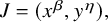 $J = (x^\beta , y^\eta ),$
which has the desired length.
$J = (x^\beta , y^\eta ),$
which has the desired length.
Case $\alpha +\beta \leq \eta $
&
$\alpha +\beta \leq \eta $
& $\beta + \eta> \alpha +1$
: If
$\beta + \eta> \alpha +1$
: If $\beta +\eta>\alpha +1$
, we go back to considering the other monomials in the ideal J. The largest y degree occurs when
$\beta +\eta>\alpha +1$
, we go back to considering the other monomials in the ideal J. The largest y degree occurs when $t=\beta -1$
, for the monomial
$t=\beta -1$
, for the monomial $x^{0}y^{\alpha +\beta -1}$
. In particular, when
$x^{0}y^{\alpha +\beta -1}$
. In particular, when $\alpha +\beta \leq \eta $
, every one of the
$\alpha +\beta \leq \eta $
, every one of the $x^{\beta -t-1} y^{2t+\alpha -\beta +1}$
is necessary. By “counting boxes,” we see that
$x^{\beta -t-1} y^{2t+\alpha -\beta +1}$
is necessary. By “counting boxes,” we see that
 $$ \begin{align*} \ell(\mathbb{K}[x,y]/J) &= (\alpha-\beta+1)\beta + \sum_{t=1}^{\beta-1} 2(\beta-t) \\ &= (\alpha-\beta+1)\beta + 2\beta(\beta-1) - (\beta-1)\beta \\ &= \beta\alpha. \end{align*} $$
Case $\alpha +\beta> \eta $
&
$\alpha +\beta> \eta $
& $\beta +\eta> \alpha +1$
: In this case, some of the monomials will become redundant with
$\beta +\eta> \alpha +1$
: In this case, some of the monomials will become redundant with $y^\eta $
. Let
$y^\eta $
. Let $t_0$
be the first index such that
$t_0$
be the first index such that $x^{\beta -t_0-1}y^{2t_0+\alpha -\beta +1}$
is redundant, that is, such that
$x^{\beta -t_0-1}y^{2t_0+\alpha -\beta +1}$
is redundant, that is, such that $2t_0+\alpha -\beta +1 \geq \eta $
. This means
$2t_0+\alpha -\beta +1 \geq \eta $
. This means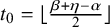 $t_0 = \lfloor \frac {\beta +\eta -\alpha }{2}\rfloor $
. We now split into cases based on the parity of
$t_0 = \lfloor \frac {\beta +\eta -\alpha }{2}\rfloor $
. We now split into cases based on the parity of $\beta + \eta - \alpha $
.
$\beta + \eta - \alpha $
.
Case: There exists $t_0$
with
$t_0$
with $\alpha -\beta +1+2t_0 = \eta $
.
$\alpha -\beta +1+2t_0 = \eta $
.

First, suppose that $2t_0+\alpha -\beta +1 = \eta $
. In this case, our set of monomials not in the ideal is depicted in Figure 1. In particular, we get
$2t_0+\alpha -\beta +1 = \eta $
. In this case, our set of monomials not in the ideal is depicted in Figure 1. In particular, we get
 $$\begin{align*}\ell(\mathbb{K}[x,y]/J) = (\alpha-\beta+1)\beta + \sum_{t=1}^{t_0} 2(\beta-t) = \beta(\alpha-\beta+1) + 2\beta t_0 -t_0(t_0+1). \end{align*}$$
Since $\alpha -\beta +1=\eta -2t_0$
and
$\alpha -\beta +1=\eta -2t_0$
and $\beta +\eta -\alpha $
is odd, this can be simplified to
$\beta +\eta -\alpha $
is odd, this can be simplified to
 $$\begin{align*}\ell(\mathbb{K}[x,y]/J) = \beta(\eta-2t_0) + 2\beta t_0-t_0(t_0+1) = \beta\eta - t_0(t_0+1) = \beta\eta - \left\lfloor\frac{(\beta+\eta-\alpha)^2}{4}\right\rfloor. \end{align*}$$
In the other case, then $2t_0+\alpha -\beta =\eta $
and our set of monomials not in the ideal is depicted in Figure 2.
$2t_0+\alpha -\beta =\eta $
and our set of monomials not in the ideal is depicted in Figure 2.
Case: There exists $t_0$
with
$t_0$
with $\alpha -\beta +2t_0 = \eta $
.
$\alpha -\beta +2t_0 = \eta $
.

In particular, we get
 $$ \begin{align*} \ell(\mathbb{K}[x,y]/J) &= (\alpha-\beta+1)\beta+\left(\sum_{t=1}^{t_0-1} 2(\beta-t)\right) + (\beta-t_0) \\ &= \beta(\alpha-\beta+1)+2\beta(t_0-1)-(t_0-1)t_0 + (\beta-t_0) \\ &= \beta(\alpha-\beta) +2\beta t_0-t_0^2. \end{align*} $$
We can again simplify using the fact that $\alpha -\beta = \eta -2t_0$
and
$\alpha -\beta = \eta -2t_0$
and $\beta +\eta -\alpha $
is even, to get
$\beta +\eta -\alpha $
is even, to get
 $$\begin{align*}\ell(\mathbb{K}[x,y]/J) = \beta(\eta-2t_0)+2\beta t_0-t_0^2 = \beta\eta - t_0^2 = \beta\eta - \left\lfloor\frac{(\beta+\eta-\alpha)^2}{4}\right\rfloor. \end{align*}$$
To simplify the statement, observe that if $\beta +\eta = \alpha +1$
, then
$\beta +\eta = \alpha +1$
, then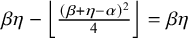 $\beta \eta - \left \lfloor \frac {(\beta +\eta -\alpha )^2}{4}\right \rfloor = \beta \eta $
, so we re-group that into case (c).
$\beta \eta - \left \lfloor \frac {(\beta +\eta -\alpha )^2}{4}\right \rfloor = \beta \eta $
, so we re-group that into case (c).
Finally, we note that there is overlap between cases (a) and (b) in the statement of the lemma, but the formula is the same—if $\alpha +\beta \leq \eta $
and
$\alpha +\beta \leq \eta $
and $\beta +\eta \leq \alpha $
, this forces
$\beta +\eta \leq \alpha $
, this forces $2\beta \leq 1$
. Since
$2\beta \leq 1$
. Since $\beta $
is an integer, this means
$\beta $
is an integer, this means $\beta =0$
.
$\beta =0$
.
Theorem 3.10 (cf. [Reference Han13, Theorem 2.3])
Let $m,n,k$
be non-negative integers such that
$m,n,k$
be non-negative integers such that $\min (m+k,m+n, n+k)\leq p$
for p a prime. Let
$\min (m+k,m+n, n+k)\leq p$
for p a prime. Let $\ell _{k,m,n}$
denote the length of the module
$\ell _{k,m,n}$
denote the length of the module $\mathbb {K}[x,y]/( x^m,y^n,(x+y)^k)$
, where
$\mathbb {K}[x,y]/( x^m,y^n,(x+y)^k)$
, where $\mathbb {K}$
is a field of either characteristic zero or characteristic p. Then,
$\mathbb {K}$
is a field of either characteristic zero or characteristic p. Then,
-
1. If
$n\geq k+m$
, then
$$\begin{align*}\ell_{k,m,n} = km.\end{align*}$$
-
2. If
$k\geq m+n$
, then
$$\begin{align*}\ell_{k,m,n}=mn.\end{align*}$$
-
3. If
$m\geq n+k$
, then
$$\begin{align*}\ell_{k,m,n} = kn.\end{align*}$$
-
4. If we are not in any of the above cases (i.e., if
$k+m>n$
and
$m+n> k$
and
$m> n+k$
), then
$$\begin{align*}\ell_{k,m,n} = kn+km+nm- \left\lfloor \frac{(k+n+m)^2}{4} \right\rfloor. \end{align*}$$


Remark 3.11. As in the proof of Theorem 3.9, there is overlap between cases (a)–(c) above, but this only occurs when one or more of $k,n$
, and m are zero.
$k,n$
, and m are zero.
Proof. Note that since $\mathbb {K}[x,y]/(x^m,y^n,(x+y)^k) \cong \mathbb {K}[x,y,z]/( x^m,y^n,z^k,x+y+z)$
, the length is unchanged by permutating
$\mathbb {K}[x,y]/(x^m,y^n,(x+y)^k) \cong \mathbb {K}[x,y,z]/( x^m,y^n,z^k,x+y+z)$
, the length is unchanged by permutating $m,n,k$
. Thus, without loss of generality, we assume that
$m,n,k$
. Thus, without loss of generality, we assume that $m+k\leq p$
and
$m+k\leq p$
and $m\leq k$
.
$m\leq k$
.
Consider the Gröbner basis found in Theorem 3.4 for when $m\leq k$
. Recall that the element
$m\leq k$
. Recall that the element $f_{2t+1}$
has leading term
$f_{2t+1}$
has leading term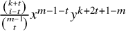 $\frac {\binom {k+t}{i-t}}{\binom {m-1}{t}}x^{m-1-t}y^{k+2t+1-m}$
. Thus, the initial term ideal of
$\frac {\binom {k+t}{i-t}}{\binom {m-1}{t}}x^{m-1-t}y^{k+2t+1-m}$
. Thus, the initial term ideal of $I_{k,m,n}$
is precisely
$I_{k,m,n}$
is precisely
 $$\begin{align*}\operatorname{\mathrm{in}} (I_{k,m,n}) = \left(x^{m-1-t}y^{k-m+1+2t} \ | \ 0\leq t \leq m-1\right) + ( x^m,y^n). \end{align*}$$
These are exactly the monomials that appeared in Theorem 3.9, so applying this lemma with $\alpha = k$
,
$\alpha = k$
, $\beta = m$
, and
$\beta = m$
, and $\eta = n$
gives the following cases:
$\eta = n$
gives the following cases:
-
(1) If
$m + n \leq k$
, then
$$\begin{align*}\ell(\mathbb{K}[x,y]/J) = m n. \end{align*}$$
-
(2) If
$k+m \leq n$
, then
$$\begin{align*}\ell(\mathbb{K}[x,y]/J) = m k. \end{align*}$$
-
(3) If
$m + n> k$
and
$k+m>n$
, then
$$\begin{align*}\ell(\mathbb{K}[x,y]/J) = m n - \left\lfloor \frac{(m+n-k)^2}{4}\right\rfloor. \end{align*}$$




The length formula in case (3) can be rewritten as
 $$ \begin{align*} m n - \left\lfloor \frac{(m+n-k)^2}{4}\right\rfloor &= \left\lceil \frac{4mn}{4} - \frac{m^2+n^2+k^2-2mk-2nk+2mn}{4} \right\rceil \\ &= \left\lceil \frac{2mk+2nk+2mn - m^2-n^2-k^2}{4}\right\rceil \\ &= \left\lceil (mk+nk+mn)-\frac{(m+n+k)^2}{4}\right\rceil\\ &= mk+nk+mn - \left\lfloor \frac{(m+n+k)^2}{4}\right\rfloor. \end{align*} $$
Via permuting $m,n,k$
, these give the cases in the original theorem statement.
$m,n,k$
, these give the cases in the original theorem statement.
4. Lengths and Gröbner bases when
$f=x^ay^b(x+y)^c$

We now return to our goal of computing the lengths of the modules of the form
 $$\begin{align*}\mathbb{F}_p [x,y]_{(x,y)}/(x^M, y^M, f^K),\end{align*}$$
where $f = x^a y^b (x+y)^c$
for non-negative integers a,
$f = x^a y^b (x+y)^c$
for non-negative integers a, $b,$
and c and positive integers
$b,$
and c and positive integers $M, K$
with
$M, K$
with $M \leq p$
. In order to make use of our previous computations in the simplified case, we will need the following lemma.
$M \leq p$
. In order to make use of our previous computations in the simplified case, we will need the following lemma.
Lemma 4.1. Suppose that $J = ( x^m, x^{a}y^bg, y^n)$
for some polynomial g in
$J = ( x^m, x^{a}y^bg, y^n)$
for some polynomial g in $\mathbb {K}[x,y]$
. Define
$\mathbb {K}[x,y]$
. Define $a'=\min (a,m)$
and
$a'=\min (a,m)$
and $b'=\min (b,n)$
, and let
$b'=\min (b,n)$
, and let $J'=( x^{m-a'}, x^{a-a'}y^{b-b'}g, y^{n-b'})$
. Then,
$J'=( x^{m-a'}, x^{a-a'}y^{b-b'}g, y^{n-b'})$
. Then,
 $$\begin{align*}\operatorname{\mathrm{in}}(J) = ( x^{m}, y^n) + x^{a'}y^{b'}\operatorname{\mathrm{in}}(J'). \end{align*}$$
In particular, we can easily find a Gröbner basis or colength for J if we have the corresponding info for $J'$
:
$J'$
:
-
1. If
$g_1, \ldots , g_s$
is a Gröbner basis for
$J'$
, then
$$\begin{align*}\{x^m, y^n\}\cup \{x^{a'}y^{b'}g_i : 1\leq i \leq s \} \end{align*}$$
is a Gröbner basis for J.
-
2. The colength of J is
$$\begin{align*}\ell(\mathbb{K}[x,y]/J) = nb' + (m-b')a'+ \ell(\mathbb{K}[x,y]/J'). \end{align*}$$


Proof. First, if either $m\leq a$
or
$m\leq a$
or $n\leq b$
, then in fact
$n\leq b$
, then in fact $J=(x^m,y^n)$
and
$J=(x^m,y^n)$
and $J'=( 1 )$
, so the statement clearly holds. Now assume
$J'=( 1 )$
, so the statement clearly holds. Now assume $m>a$
and
$m>a$
and $n>b$
, so that
$n>b$
, so that $J' = (x^{m-a},\, g,\, y^{n-b})$
.
$J' = (x^{m-a},\, g,\, y^{n-b})$
.
First, we show that the RHS is contained in the LHS. The monomials $x^m$
and
$x^m$
and $y^n$
are both clearly contained in
$y^n$
are both clearly contained in $\operatorname {\mathrm {in}}(J)$
. Further, consider any
$\operatorname {\mathrm {in}}(J)$
. Further, consider any $h = h_0x^{m-a}+h_1g + h_2y^{n-b}\in J'$
, so that
$h = h_0x^{m-a}+h_1g + h_2y^{n-b}\in J'$
, so that $\operatorname {\mathrm {in}}(h)\in \operatorname {\mathrm {in}}(J')$
. Thus,
$\operatorname {\mathrm {in}}(h)\in \operatorname {\mathrm {in}}(J')$
. Thus, $\operatorname {\mathrm {in}}(x^ay^bh) = (h_0y^b)x^m + (x^ay^bh_1)g + (h_2x^a)y^n\in \operatorname {\mathrm {in}}(J)$
.
$\operatorname {\mathrm {in}}(x^ay^bh) = (h_0y^b)x^m + (x^ay^bh_1)g + (h_2x^a)y^n\in \operatorname {\mathrm {in}}(J)$
.
Now, we show that the LHS is contained in the RHS. Take any $h\in J$
, writing
$h\in J$
, writing $h=h_0x^m+ h_1x^ay^bg+h_2y^n$
. Use the Euclidean algorithm to write
$h=h_0x^m+ h_1x^ay^bg+h_2y^n$
. Use the Euclidean algorithm to write $h_0 = q_0 y^b + r_0$
and
$h_0 = q_0 y^b + r_0$
and $h_2 = q_2x^a+r_2$
, so that
$h_2 = q_2x^a+r_2$
, so that
 $$\begin{align*}h=x^ay^b(q_0x^m+h_1g+q_2y^n) + r_0x^m+ r_2y^n. \end{align*}$$
In particular, no term of $r_0x^m$
can cancel with any other term, because no term of
$r_0x^m$
can cancel with any other term, because no term of $r_0$
is divisible by
$r_0$
is divisible by $y^b$
; and similarly for
$y^b$
; and similarly for $r_2y^n$
. Thus, we have three cases:
$r_2y^n$
. Thus, we have three cases:
-
•
$\operatorname {\mathrm {in}}(h) = \operatorname {\mathrm {in}}(r_0x^m)$
: Then,
$\operatorname {\mathrm {in}}(h)\in ( x^m,y^n)$
. -
•
$\operatorname {\mathrm {in}}(h) = \operatorname {\mathrm {in}}(r_2y^n)$
: Then,
$\operatorname {\mathrm {in}}(h)\in ( x^m,y^n)$
. -
•
$\operatorname {\mathrm {in}}(h) = \operatorname {\mathrm {in}}(x^ay^b(q_0x^m+h_1g+q_2y^n))$
: Since
$q_0x^m+h_1g+q_2y^n\in J'$
, we have
$\operatorname {\mathrm {in}}(h) \in x^ay^b\operatorname {\mathrm {in}}(J')$
.







For the Gröbner basis conclusion, first note that the proposed basis elements are all contained in J. By the above discussion, their initial terms also generate the initial ideal of J and thus form a Gröbner basis as desired.
For the length conclusion, we use that $\mathbb {K}[x,y]/J$
and
$\mathbb {K}[x,y]/J$
and $\mathbb {K}[x,y]/\operatorname {\mathrm {in}}(J)$
have the same Hilbert function, and that the colength of a monomial ideal can be determined by “counting boxes.” More specifically, multiplying by
$\mathbb {K}[x,y]/\operatorname {\mathrm {in}}(J)$
have the same Hilbert function, and that the colength of a monomial ideal can be determined by “counting boxes.” More specifically, multiplying by $x^{a'}y^{b'}$
shifts the diagram for
$x^{a'}y^{b'}$
shifts the diagram for $\mathbb {K}[x,y]/\operatorname {\mathrm {in}}(J')$
up by
$\mathbb {K}[x,y]/\operatorname {\mathrm {in}}(J')$
up by $b'$
and to the right by
$b'$
and to the right by $a'$
. See Figure 3 for an illustration.
$a'$
. See Figure 3 for an illustration.
The diagram of monomials in $\mathbb {K}[x,y]/\operatorname {\mathrm {in}}(J)$
. The diagram for
$\mathbb {K}[x,y]/\operatorname {\mathrm {in}}(J)$
. The diagram for $\mathbb {K}[x,y]/\operatorname {\mathrm {in}}(J')$
is the “triangular” region in the upper right.
$\mathbb {K}[x,y]/\operatorname {\mathrm {in}}(J')$
is the “triangular” region in the upper right.
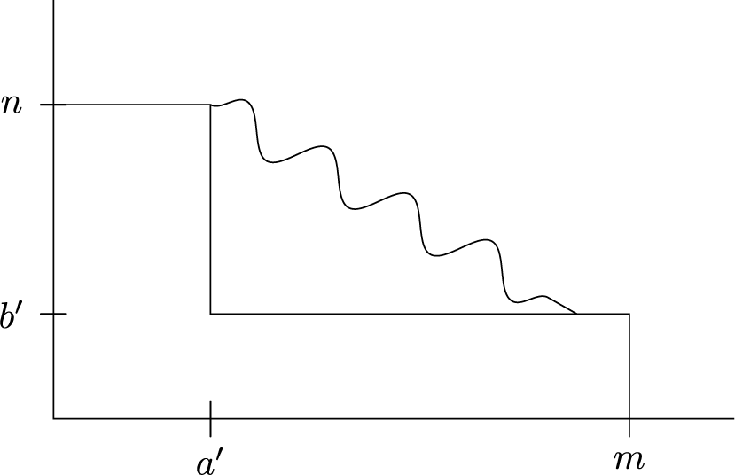
We will now use Theorem 4.1 to extend the Gröbner basis and lengths we computed in Section 3 when $f=x+y$
to the case when
$f=x+y$
to the case when $f=x^ay^b(x+y)^c$
.
$f=x^ay^b(x+y)^c$
.
Proposition 4.2. Consider the ideal $I=(x^M, y^N, f^K)$
in
$I=(x^M, y^N, f^K)$
in $\mathbb {K}[x,y]$
, where
$\mathbb {K}[x,y]$
, where $f=x^ay^b(x+y)^c$
and where
$f=x^ay^b(x+y)^c$
and where $M,N,K,a,b,c$
are all non-negative integers. Assume that the field
$M,N,K,a,b,c$
are all non-negative integers. Assume that the field $\mathbb {K}$
has either characteristic zero, or characteristic p where
$\mathbb {K}$
has either characteristic zero, or characteristic p where $M+(c-a)K \leq p$
.
$M+(c-a)K \leq p$
.
-
1. If either
$aK \geq M$
or
$bK\geq N$
, then
$$\begin{align*}\{x^M,y^N\} \end{align*}$$
is a Gröbner basis for I.
-
2. If
$aK<M, bK<N$
, and
$(a+c)K\geq M$
, then
$$\begin{align*}\{x^M,\, y^N\} \cup \left\{ H_t : 0\leq t < M-aK \right\} \end{align*}$$
is a Gröbner basis for I, where
$$\begin{align*}H_t = \sum_{j=0}^{M-aK-t-1} \left(\prod_{\ell=1}^t\frac{M-aK-j-\ell}{M-aK-\ell}\right) \binom{cK+t}{j} x^{aK+j}y^{(b+c)K-j+t}. \end{align*}$$
Thus, I has initial ideal
$$\begin{align*}\operatorname{\mathrm{in}}(I) = (x^M,\, y^N) + \left( x^{M-t-1}y^{(a+b+c)K-M+2t+1} : 0\leq t < M-aK \right). \end{align*}$$
-
3. Finally, if
$aK<M$
,
$bK<N$
, and
$(a+c)K<M,$
then
$$\begin{align*}\{x^M,\, y^N,\, x^{aK}y^{bK}(x+y)^{cK}\} \cup \left\{ L_t : 0\leq t < cK \right\} \end{align*}$$
is a Gröbner basis for I, where
$$\begin{align*}L_t = \sum_{i=0}^{cK-1-t}\left(\sum_{j=i}^{cK-1-t} (-1)^{M-aK-j-t} \left(\frac{\prod_{\ell=1}^t(cK-j-\ell)}{\prod_{\ell=1}^t(cK-\ell)}\right) \binom{M-aK+t}{j}\binom{j}{i} \right) x^{i+aK} y^{M+(b-a)K-i+t}. \end{align*}$$
Thus, I has initial ideal
$$\begin{align*}\operatorname{\mathrm{in}}(I) = ( x^M,\, y^N,\, x^{(a+c)K}y^{bK}) + \left( x^{(a+c)K-t-1} y^{M+(b-a-c)K+2t+1} : 0\leq t < cK \right). \end{align*}$$









Proof. The first case is clear. For the second case, combine Theorems 3.4 and 4.1. For the last case, combine Theorems 3.8 and 4.1. The constraint inequalities come from setting $m=M-aK$
,
$m=M-aK$
, $n=M-bK$
, and
$n=M-bK$
, and $k=cK$
.
$k=cK$
.
We can now compute our desired lengths.
Theorem 4.3. Suppose $f=x^ay^b(x+y)^c$
is a polynomial in
$f=x^ay^b(x+y)^c$
is a polynomial in $\mathbb {K}[x,y]$
for non-negative integers
$\mathbb {K}[x,y]$
for non-negative integers $a,b,c$
, and let
$a,b,c$
, and let $M,K$
be fixed positive integers such that
$M,K$
be fixed positive integers such that $aK,bK \leq M$
. Assume the field
$aK,bK \leq M$
. Assume the field $\mathbb {K}$
has either characteristic
$\mathbb {K}$
has either characteristic $0$
or characteristic
$0$
or characteristic $p,$
where
$p,$
where
 $$\begin{align*}\min\{M+(c-a)K,\ M+(c-b)K,\ 2M-(a+b)K\}\leq p.\end{align*}$$
Let $\ell _{K,M}$
denote the length of the module
$\ell _{K,M}$
denote the length of the module $\mathbb {K}[x,y]/( x^M,y^M,f^K)$
.
$\mathbb {K}[x,y]/( x^M,y^M,f^K)$
.
-
1. If
$a\geq b+c$
, then
$$\begin{align*}\ell_{K,M} = (a+b+c)KM-a(b+c)K^2.\end{align*}$$
-
2. If
$(a+b+c)K\geq 2M$
, then
$$\begin{align*}\ell_{K,M} = M^2.\end{align*}$$
-
3. If
$b\geq a+c,$
then
$$\begin{align*}\ell_{K,M} = (a+b+c)KM-b(a+c)K^2.\end{align*}$$
-
4. If we are not in cases (a)–(c), then
$$\begin{align*}\ell_{K,M} = (a+b+c)KM - \left\lfloor \frac{(a+b+c)^2K^2}{4} \right\rfloor.\end{align*}$$





Proof. Theorem 4.1 using $m=M-aK$
,
$m=M-aK$
, $n=M-bK$
, and
$n=M-bK$
, and $k=cK$
gives
$k=cK$
gives
 $$\begin{align*}\ell_{K,M} = M(bK)+(M-bK)aK+\ell_{cK,M-aK,M-bK} = (a+b)KM -abK^2+\ell_{cK,M-aK,M-bK}.\end{align*}$$
Now, we use Theorem 3.10 to get $\ell _{cK,M-aK,M-bK}$
and then simplify:
$\ell _{cK,M-aK,M-bK}$
and then simplify:
-
1. The condition
$(M-bK) \geq cK+(M-aK)$
is equivalent to
$a\geq b+c$
, and gives
$\ell _{cK,M-aK,M-bK} = cK(M-aK)$
. Therefore,
$$\begin{align*}\ell_{K,M} = (a+b+c)KM - a(b+c)K^2. \end{align*}$$
-
2. The condition
$cK\geq (M-aK)+(M-bK)$
is equivalent to
$(a+b+c)K\geq 2M$
, and gives
$\ell _{cK,M-aK,M-bK} = (M-aK)(M-bK)$
. Therefore,
$$\begin{align*}\ell_{K,M} = M^2. \end{align*}$$
-
3. The condition
$(M-aK)\geq (M-bK)+cK$
is equivalent to
$b\geq a+c$
, and gives
$\ell _{cK,M-aK,M-bK} = cK(M-bK)$
. Therefore,
$$\begin{align*}\ell_{K,M} = (a+b+c)KM - b(a+c)K^2. \end{align*}$$
-
4. If we are not in any of these cases, then
$\ell _{cK,M-aK,M-bK}$
is
$$ \begin{align*} &cK(M-bK)+cK(M-aK)+(M-aK)(M-bK)- \left\lfloor \frac{(cK+(M-bK)+(M-aK))^2}{4} \right\rfloor\\ &\quad= M^2 + (2c-a-b)KM +(ab-ac-bc)K^2 - \left\lfloor \frac{4M^2+4(c-a-b)KM + (c-a-b)^2K^2}{4} \right\rfloor. \end{align*} $$
Therefore,
$$ \begin{align*} \ell_{K,M} &= M^2 +2cKM -c(a+b)K^2 - \left\lfloor \frac{4M^2+4(c-a-b)KM + (c-a-b)^2K^2}{4} \right\rfloor\\ &= (a+b+c)KM - \left\lfloor \frac{(a+b+c)^2K^2}{4} \right\rfloor. \end{align*} $$















Remark 4.4. When $M = p$
and
$M = p$
and $\mathbb {K}$
has characteristic
$\mathbb {K}$
has characteristic $p>0$
in Theorem 4.3, the hypotheses can be simplified: in this case, the ideals
$p>0$
in Theorem 4.3, the hypotheses can be simplified: in this case, the ideals $(x^p, y ^p, (x^a y ^b (x+y) ^c)^K)$
and
$(x^p, y ^p, (x^a y ^b (x+y) ^c)^K)$
and $(x^p, y ^p, (x^c y ^b (x+y) ^a)^K)$
are related by a linear change of coordinates, and hence have the same co-length. Thus, we may permute
$(x^p, y ^p, (x^c y ^b (x+y) ^a)^K)$
are related by a linear change of coordinates, and hence have the same co-length. Thus, we may permute $a,b$
, and c to assume that
$a,b$
, and c to assume that $c \leq a $
, in which case, the hypothesis now becomes simply
$c \leq a $
, in which case, the hypothesis now becomes simply $ aK \leq p$
and
$ aK \leq p$
and $bK \leq p$
, with no need to consider the minimum.
$bK \leq p$
, with no need to consider the minimum.
5. Connections to Lefschetz properties
We now present an alternate perspective on computing the lengths in Section 3.3. In the setting of Section 3, we can re-express our length $\ell _{k,m,n}$
as
$\ell _{k,m,n}$
as
 $$\begin{align*}\ell_{k,m,n} = \ell\left(\mathbb{K}[x,y]/( x^m,y^n,(x+y)^k) \right) = \ell\left(\mathbb{K}[x,y,z]/( x^m,y^n,z^k,x+y+z) \right). \end{align*}$$
This suggests a connection to the WLP: recall that a standard graded Artinian F-algebra S has the WLP if there is a linear form $L\in S_1$
such that for all degrees j, the multiplication map
$L\in S_1$
such that for all degrees j, the multiplication map $\times L: S_{j-1} \to S_{j}$
has maximal rank. Such an
$\times L: S_{j-1} \to S_{j}$
has maximal rank. Such an ${\widehat {\rm vol}}L$
is a weak Lefschetz element. Further, in the case that
${\widehat {\rm vol}}L$
is a weak Lefschetz element. Further, in the case that $S=\mathbb {K}[x_1,\ldots , x_n]/I$
for I monomial, it suffices to check whether
$S=\mathbb {K}[x_1,\ldots , x_n]/I$
for I monomial, it suffices to check whether $L=x_1+ \cdots + x_n$
has this property [Reference Lundqvist and Nicklasson23, Prop. 4.3].
$L=x_1+ \cdots + x_n$
has this property [Reference Lundqvist and Nicklasson23, Prop. 4.3].
Lemma 5.1. Let S be a standard graded Artinian, Gorenstein $\mathbb {K}$
-algebra, where
$\mathbb {K}$
-algebra, where $\mathbb {K}$
is an algebraically closed field. If L is a weak Lefschetz element for S, then
$\mathbb {K}$
is an algebraically closed field. If L is a weak Lefschetz element for S, then
 $$\begin{align*}\ell(S/LS) = \dim_{\mathbb{K}}(S_{\lfloor t/2\rfloor}), \end{align*}$$
where t is the socle degree of S.
Proof. Since L is homogeneous, we can decompose

Since L is a weak Lefschetz element, these maps are injective up until some degree, from which point on they switch to becoming surjective, by [Reference Migliore, Miró-Roig and Nagel26, Prop. 2.1]. Since S is standard graded Gorenstein, $\dim _{\mathbb {K}} S_j = \dim _{\mathbb {K}} S_{t-j}$
and so this symmetry forces the switch point to be at
$\dim _{\mathbb {K}} S_j = \dim _{\mathbb {K}} S_{t-j}$
and so this symmetry forces the switch point to be at $\lfloor t/2\rfloor $
. So
$\lfloor t/2\rfloor $
. So

Consider the following result of Lundqvist and Nicklasson (which extends an earlier result of Cook II [Reference Cook12, Prop. 3.5]), stated here in the three-variable case.
Theorem 5.2 [Reference Lundqvist and Nicklasson23, Thm. 4.4]
Let $R=\mathbb {K}[x_0,x_1,x_2]$
, where
$R=\mathbb {K}[x_0,x_1,x_2]$
, where $\mathbb {K}$
is a field of characteristic
$\mathbb {K}$
is a field of characteristic $p>0$
. Let
$p>0$
. Let $d_0\geq d_1\geq d_2\geq 1$
and let
$d_0\geq d_1\geq d_2\geq 1$
and let $t=\sum _{i=0}^2 (d_i-1)$
. If
$t=\sum _{i=0}^2 (d_i-1)$
. If $\max (p,d_0)>\frac {t+1}{2}$
, then
$\max (p,d_0)>\frac {t+1}{2}$
, then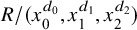 $R/( x_0^{d_0}, x_1^{d_1}, x_2^{d_2})$
has the WLP.
$R/( x_0^{d_0}, x_1^{d_1}, x_2^{d_2})$
has the WLP.
We can now use this to compute $\ell _{k,m,n}$
directly, as the following result shows.
$\ell _{k,m,n}$
directly, as the following result shows.
Theorem 5.3. Suppose $\{k,m,n\} = \{d_0\geq d_1\geq d_2\}$
, and let
$\{k,m,n\} = \{d_0\geq d_1\geq d_2\}$
, and let $t=k+m+n-3$
. Suppose
$t=k+m+n-3$
. Suppose $\mathbb {K}$
is a field of characteristic
$\mathbb {K}$
is a field of characteristic $p,$
where p is a positive prime, and assume
$p,$
where p is a positive prime, and assume $0\leq m,n\leq p-k$
. Then,
$0\leq m,n\leq p-k$
. Then,
-
1. If
$d_0 \leq \lceil \frac {t}{2}\rceil $
, that is, if
$2d_0\leq t+1$
, then
$$\begin{align*}\ell_{k,m,n} = \binom{\lfloor t/2\rfloor+2}{2} - \sum_{i=0}^2 \binom{\lfloor t/2\rfloor - d_i +2}{2}. \end{align*}$$
-
2. If
$d_0> \lceil \frac {t}{2}\rceil $
, that is, if
$\,2d_0>t+1$
, then
$$\begin{align*}\ell_{k,m,n} = d_1d_2. \end{align*}$$


Proof. The starting assumption of $0\leq m,n\leq p-k$
means that
$0\leq m,n\leq p-k$
means that $t=m+n+k-3 \leq p+n-3\leq 2p-k-3$
. But then
$t=m+n+k-3 \leq p+n-3\leq 2p-k-3$
. But then
 $$\begin{align*}\left\lceil \frac{t+1}{2}\right\rceil \leq \left\lceil \frac{2p-k-2}{2}\right\rceil = p-1-\left\lfloor \frac{k}{2}\right\rfloor < p. \end{align*}$$
Thus, $S=\mathbb {K}[x,y,z]/ (x^m,y^n,z^k)$
has the WLP. From here, we handle each case separately.
$S=\mathbb {K}[x,y,z]/ (x^m,y^n,z^k)$
has the WLP. From here, we handle each case separately.
-
1. Since S has the WLP, this means
$$\begin{align*}\ell_{k,m,n} = \ell(S/(x+y+z)S) = \dim_{\mathbb{K}} (S_{\lfloor t/2\rfloor}). \end{align*}$$
Further, we in general know that
$\dim _{\mathbb {K}}(\mathbb {K}[x,y,z])_i = \binom {i+2}{2}$
, and by inclusion–exclusion, that
$\dim _{\mathbb {K}}(( x_0^{d_0},x_1^{d_1},x_2^{d_2}))_i$
is
$$\begin{align*}\left(\sum_{j=0}^2\binom{i-d_j+2}{2} \right) - \left(\sum_{0\leq j < j'\leq 2}\binom{i-d_j-d_{j'}+2}{2} \right) + \binom{i-d_0-d_1-d_2+2}{2}. \end{align*}$$
However, since
$d_2\leq d_1\leq d_0 \leq \lceil t/2\rceil $
, this means that
$$\begin{align*}\left\lfloor \frac{t}{2}\right\rfloor - d_j - d_{j'}+2 = \left\lfloor \frac{t}{2}\right\rfloor +d_{j"}-t-1 = d_{j"} - \left\lceil \frac{t}{2}\right\rceil - 1<0. \end{align*}$$
Thus,
$$\begin{align*}\dim_{\mathbb{K}}(( x_0^{d_0},x_1^{d_1},x_2^{d_2}))_{\lfloor t/2\rfloor} = \left(\sum_{j=0}^2\binom{\lfloor t/2\rfloor-d_j+2}{2}\right). \end{align*}$$
Now subtracting gives our desired result.
-
2. In this case, we return to our original two-variable perspective. We can by change of variables assume that
$k=d_0$
, and rewrite the inequality as
$k> \lceil \frac {k+m+n-3}{2}\rceil $
. This implies that
$2k>(k+m+n-3)+1$
, that is, that
$k\geq m+n-1$
. This then ensures that
$(x+y)^k \in ( x^m, y^n)$
, and so
$$\begin{align*}\ell_{k,m,n} = \ell(\mathbb{K}[x,y]/( x^m,y^n)) = mn = d_1d_2.\\[-41pt] \end{align*}$$







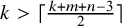




Remark 5.4. By expanding out the formula in case (a), we get that the length $\ell _{k,m,n}$
is
$\ell _{k,m,n}$
is
 $$\begin{align*}&-\left\lfloor \frac{d_0+d_1+d_2+1}{2}\right\rfloor^2 {\kern-1pt}+{\kern-1pt} (d_0+d_1+d_2+1){\kern-1pt} \left\lfloor \frac{d_0+d_1+d_2+1}{2}\right\rfloor- \frac{(d_0+1)d_0+(d_1+1)d_1+(d_2+1)d_2}{2}. \end{align*}$$
Since in general $w\cdot \lfloor n/2\rfloor - \lfloor w/2\rfloor ^2 = \lfloor w^2/4\rfloor $
, we can combine and simplify the above to
$w\cdot \lfloor n/2\rfloor - \lfloor w/2\rfloor ^2 = \lfloor w^2/4\rfloor $
, we can combine and simplify the above to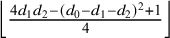 $\left \lfloor \frac {4d_1d_2-(d_0-d_1-d_2)^2+1}{4}\right \rfloor $
, which can be directly checked to be the same as the formula we got in Theorem 3.10.
$\left \lfloor \frac {4d_1d_2-(d_0-d_1-d_2)^2+1}{4}\right \rfloor $
, which can be directly checked to be the same as the formula we got in Theorem 3.10.
Remark 5.5. The referee pointed out to us that Han computes the same length formulas as above, but with the assumption that $(x+y)^k$
is a non-zero divisor on the degree
$(x+y)^k$
is a non-zero divisor on the degree $\frac {\lfloor m+n-k-2\rfloor }{2}$
component of
$\frac {\lfloor m+n-k-2\rfloor }{2}$
component of $\mathbb K[x,y]/(x^m,y^n)$
(see [Reference Han13, Thm. 2.3]). Recently, Nicklasson [Reference Nicklasson31, Thm. 3.2] has classified monomial complete intersections in two variables with the strong Lefschetz property (SLP) (also see Cook II [Reference Cook12, Cor. 4.8] for the characteristic
$\mathbb K[x,y]/(x^m,y^n)$
(see [Reference Han13, Thm. 2.3]). Recently, Nicklasson [Reference Nicklasson31, Thm. 3.2] has classified monomial complete intersections in two variables with the strong Lefschetz property (SLP) (also see Cook II [Reference Cook12, Cor. 4.8] for the characteristic $2$
case), which confirms Han’s assumption whenever
$2$
case), which confirms Han’s assumption whenever $m,n,k,p$
satisfy the hypothesis of Theorem 5.3. This yields a third computation of the lengths in Theorem 3.10.
$m,n,k,p$
satisfy the hypothesis of Theorem 5.3. This yields a third computation of the lengths in Theorem 3.10.
6. Limit F-signature
In this section, we will use the computation of the lengths from Theorem 4.3 to compute the limit F-signature functions of the polynomials $f= x^a y^b (x+y)^c$
and
$f= x^a y^b (x+y)^c$
and $g = x^a y^b (x^u + y^v)^c $
for non-negative integers a, b, c, u, and v. In what follows, by abuse of notation, we view the polynomials in rings of varying characteristics, which is well-defined since f and g have coefficients in
$g = x^a y^b (x^u + y^v)^c $
for non-negative integers a, b, c, u, and v. In what follows, by abuse of notation, we view the polynomials in rings of varying characteristics, which is well-defined since f and g have coefficients in ${\mathbb {Z}}$
.
${\mathbb {Z}}$
.
Theorem 6.1. Assume $a \geq b \geq c \geq 0$
are non-negative integers. Let
$a \geq b \geq c \geq 0$
are non-negative integers. Let $\psi (t)$
be the limit F-signature function of
$\psi (t)$
be the limit F-signature function of $f = x^a y^b (x+y)^c$
, so that
$f = x^a y^b (x+y)^c$
, so that
 $$\begin{align*}\psi(t) = \lim_{p\to\infty} s_p(\mathbb{F}_p[x,y]_{( x,y)}, f^t). \end{align*}$$
Let $\lambda = \operatorname {\mathrm {lct}}(f)$
. Then, for any real number
$\lambda = \operatorname {\mathrm {lct}}(f)$
. Then, for any real number $t \geq 0$
, we have:
$t \geq 0$
, we have:
-
1. If
$t \geq \lambda $
, then
$\psi (t) = 0$
. -
2. If
$t< \lambda $
and
$a\geq b+c$
, then
$\psi (t) = (1 - at) (1 - (b+c)t)$
. -
3. If
$t < \lambda $
and
$a < b+c$
, then
$\psi (t) = \left ( 1 - \frac {(a+b+c)}{2}t \right )^2$
.





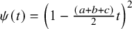
In other words, when $a \geq b+c$
, we have
$a \geq b+c$
, we have
 $$\begin{align*}\psi(t) = \begin{cases} (1-at)(1-(b+c)t) & 0 \leq t < \frac{1}{a} \\ 0 & t \geq \frac{1}{a} \end{cases}, \end{align*}$$
and when $a < b+c,$
we have
$a < b+c,$
we have
 $$\begin{align*}\psi(t) = \begin{cases} \left(1-\frac{(a+b+c)}{2}t\right)^2 & 0 \leq t < \frac{2}{a+b+c} \\ 0 & t \geq \frac{2}{a+b+c} \end{cases}. \end{align*}$$
We first observe what happens in the $c=0$
case before diving into the full proof.
$c=0$
case before diving into the full proof.
Lemma 6.2. Fix non-negative integers $a, b \geq 0$
. Then, for any non-negative real parameter
$a, b \geq 0$
. Then, for any non-negative real parameter $t \geq 0$
, the F-signature function of the pair
$t \geq 0$
, the F-signature function of the pair $(\mathbb {F}_p [x,y]_{(x,y)} , (x^{a} y^{b})^t)$
, denoted by
$(\mathbb {F}_p [x,y]_{(x,y)} , (x^{a} y^{b})^t)$
, denoted by $\psi _p (t)$
, is given by
$\psi _p (t)$
, is given by
 $$\begin{align*}\psi_p(t) = \begin{cases} (1-at)(1-bt) & 0\leq t < \min\{\frac{1}{a},\ \frac{1}{b}\} \\ 0 & t \geq \min\{\frac{1}{a},\ \frac{1}{b}\} \end{cases}.\end{align*}$$
Proof. See [Reference Blickle, Schwede and Tucker6, Example 4.19].
Proof of Theorem 6.1
To check that our proposed piecewise formula is indeed the same as our proposed list of cases, observe first by an easy computation after blowing up the origin that $\lambda = \operatorname {\mathrm {lct}}(f) = \min \{\frac {1}{a}, \frac {2}{a+b+c} \}.$
Therefore, we see that
$\lambda = \operatorname {\mathrm {lct}}(f) = \min \{\frac {1}{a}, \frac {2}{a+b+c} \}.$
Therefore, we see that $1/a$
is the minimum exactly when
$1/a$
is the minimum exactly when $a+b+c\leq 2a$
, equivalently when
$a+b+c\leq 2a$
, equivalently when $a\geq b+c$
.
$a\geq b+c$
.
Let $\phi (t)$
denote the candidate formula for the limit F-signature. In other words, if
$\phi (t)$
denote the candidate formula for the limit F-signature. In other words, if $a \leq b+c,$
then
$a \leq b+c,$
then $\lambda = \frac {2}{a+b+c}$
and for
$\lambda = \frac {2}{a+b+c}$
and for $ t \geq 0$
,
$ t \geq 0$
,
 $$\begin{align*}\phi(t) = \begin{cases} \left(1-\frac{(a+b+c)}{2}t\right)^2 & 0 \leq t < \frac{2}{a+b+c} \\ 0 & t \geq \frac{2}{a+b+c} \end{cases}.\end{align*}$$
Similarly, if $a> b+c,$
then
$a> b+c,$
then $\lambda = \frac {1}{a}$
and for
$\lambda = \frac {1}{a}$
and for $t \geq 0$
, we have
$t \geq 0$
, we have
 $$\begin{align*}\phi(t) = \begin{cases} (1-at)(1-(b+c)t) & 0 \leq t < \frac{1}{a} \\ 0 & t \geq \frac{1}{a} \end{cases}. \end{align*}$$
Note that in either case, the function $\phi (t)$
is continuous and non-increasing. Our goal is to prove that
$\phi (t)$
is continuous and non-increasing. Our goal is to prove that $\phi (t)=\psi (t)$
. For notational convenience, let
$\phi (t)=\psi (t)$
. For notational convenience, let
 $$\begin{align*}\psi_{p} (t) = s_{p}(\mathbb{F}_p[x,y]_{(x,y)}, \, f ^{t}). \end{align*}$$
If $c=0$
, then
$c=0$
, then $a\geq b$
and we are in the case of Theorem 6.2 which clearly matches our proposed
$a\geq b$
and we are in the case of Theorem 6.2 which clearly matches our proposed $\phi (t)$
. So now assume
$\phi (t)$
. So now assume $c> 0$
.
$c> 0$
.
For any $t>0$
and prime numbers p, write
$t>0$
and prime numbers p, write $r_p = \lfloor tp \rfloor $
so that
$r_p = \lfloor tp \rfloor $
so that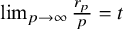 $\lim _{p \to \infty } \frac {r_p} {p} = t$
. By Theorem 2.5, to compute the limit F-signature function
$\lim _{p \to \infty } \frac {r_p} {p} = t$
. By Theorem 2.5, to compute the limit F-signature function $\psi (t)$
(and show that it exists), it suffices to show that
$\psi (t)$
(and show that it exists), it suffices to show that $\lim _{p \to \infty } \psi _p (\frac {r_p}{p}) = \phi (t)$
. This is clear when
$\lim _{p \to \infty } \psi _p (\frac {r_p}{p}) = \phi (t)$
. This is clear when $t \geq \lambda $
, since then
$t \geq \lambda $
, since then $t \geq \operatorname {\mathrm {{fpt}}}(f)$
(see Theorems 2.2 and 2.3) and thus
$t \geq \operatorname {\mathrm {{fpt}}}(f)$
(see Theorems 2.2 and 2.3) and thus $\psi _p (t) = 0$
for all p. So we now fix a t with
$\psi _p (t) = 0$
for all p. So we now fix a t with $\lambda> t >0$
, and define
$\lambda> t >0$
, and define $r_p$
as above.
$r_p$
as above.
Let $S_p$
denote the ring
$S_p$
denote the ring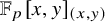 $\mathbb {F}_p [x,y]_{(x,y)}$
. Then, by Equation (2.1.1), we have
$\mathbb {F}_p [x,y]_{(x,y)}$
. Then, by Equation (2.1.1), we have
 $$\begin{align*}\psi_p \left(\frac{r_p}{p}\right) = \frac{1}{p^2} \ell_{S_p}(S_p/(\mathfrak{m}^{[p]} : f^{r_p})). \end{align*}$$
By the exact sequence,
 $$\begin{align*}0 \to S_p/(\mathfrak{m}^{[p]} : f^{r_p}) \to S_p /\mathfrak{m}^{[p]} \to S_p/(\mathfrak{m}^{[p]}, f^{r_p}) \to 0, \end{align*}$$
where the left map is given by multiplication by $f^{r_p}$
, we see that
$f^{r_p}$
, we see that
 $$\begin{align*}\psi_p\left(\frac{r_p}{p}\right) = 1 - \frac{1}{p^2} \ell_{S_p}(S_p/(x^p, y^p, f^{r_p})). \end{align*}$$
Thus, to prove the theorem, it suffices to show that
 $$ \begin{align} \lim_{p \to \infty} \frac{\ell_{S_p}(S_p/(x^p,y^p, f^{r_p}))}{p^2} = 1 - \phi(t) .\end{align} $$
We will check this using the lengths computed in Theorem 4.3. Since we have assumed that $0<t < \lambda \leq \frac {1}{a}$
, for all
$0<t < \lambda \leq \frac {1}{a}$
, for all $p \gg 0,$
we have
$p \gg 0,$
we have $r_p>0$
and also
$r_p>0$
and also $r_p \, b \leq r_p \, a \leq p$
. Thus, we may apply Theorem 4.3 with
$r_p \, b \leq r_p \, a \leq p$
. Thus, we may apply Theorem 4.3 with $M = p$
and
$M = p$
and $K = r_p$
(see Theorem 4.4).
$K = r_p$
(see Theorem 4.4).
First consider the case when $a\geq b+c$
, which is part (a) of Theorem 4.3. Then, the length formula gives
$a\geq b+c$
, which is part (a) of Theorem 4.3. Then, the length formula gives
 $$\begin{align*}\lim_{p \to \infty} \frac{\ell_{S_p}(S_p/(x^p,y^p, f^{r_p}))}{p^2} = \lim_{p \to \infty} \frac{(a+b+c)r_p \, p - a(b+c)r_p ^2}{p^2} = (a+b+c)t - a(b+c)t^2, \end{align*}$$
which is easily seen to be equal to $1 - (1 - at) (1 - (b+c)t)$
.
$1 - (1 - at) (1 - (b+c)t)$
.
Next, assume $a<b+c$
and
$a<b+c$
and $t<\lambda $
. Since
$t<\lambda $
. Since $t<\frac {2}{a+b+c}$
, this means for all
$t<\frac {2}{a+b+c}$
, this means for all $p\gg 0$
, we have
$p\gg 0$
, we have $r_p(a+b+c) < 2p$
. Since also
$r_p(a+b+c) < 2p$
. Since also $a\geq b$
, we must be in part (d) of Theorem 4.3. Thus, we have
$a\geq b$
, we must be in part (d) of Theorem 4.3. Thus, we have
 $$ \begin{align*} \lim_{p\to\infty} \frac{\ell_{S_p}(S_p/( x^p,y^p,f^{r_p}))}{p^2} &= \lim_{p\to\infty} \frac{(a+b+c)r_p p -\left\lfloor \frac{(a+b+c)^2r_p^2}{4} \right\rfloor}{p^2} \\ &= (a+b+c)t - \frac{(a+b+c)^2t^2}{4} \\ &= 1 - \left(1-\frac{(a+b+c)}{2}t\right)^2 \end{align*} $$
as required. This completes the proof.
Remark 6.3. Given three positive rational numbers $r_1$
,
$r_1$
, $r_2$
, and
$r_2$
, and $r_3$
, it is possible to choose integers
$r_3$
, it is possible to choose integers $a,b,c$
and a rational number
$a,b,c$
and a rational number $t>0$
such that
$t>0$
such that $r_1 = at$
,
$r_1 = at$
, $r_2 = bt$
, and
$r_2 = bt$
, and $r_3 = ct$
. Thus, Theorem 6.1 can be used to compute the limit F-signature of
$r_3 = ct$
. Thus, Theorem 6.1 can be used to compute the limit F-signature of $x^{r_1} y^{r_2} (x+y)^{r_3}$
for any three positive rational numbers
$x^{r_1} y^{r_2} (x+y)^{r_3}$
for any three positive rational numbers $r_1$
,
$r_1$
, $r_2$
,
$r_2$
, $r_3$
. Moreover, the cases in the statement of Theorem 6.1 depend only on the
$r_3$
. Moreover, the cases in the statement of Theorem 6.1 depend only on the $r_i$
and not on the specific choices of a, b, c, and t. Therefore, if we assume
$r_i$
and not on the specific choices of a, b, c, and t. Therefore, if we assume $r_1 \geq r_2 \geq r_3$
and let
$r_1 \geq r_2 \geq r_3$
and let $s_\infty $
denote the limit F-signature of the pair
$s_\infty $
denote the limit F-signature of the pair $({\mathbb {Z}}[x,y], x^{r_1} y^{r_2} (x+y) ^{r_3})$
, then Theorem 6.1 gives:
$({\mathbb {Z}}[x,y], x^{r_1} y^{r_2} (x+y) ^{r_3})$
, then Theorem 6.1 gives:
-
1. If
$r_1 + r_2 + r_3 \geq 2$
or
$r_1 \geq 1$
, then
$s_\infty = 0$
. -
2. If
$r_1 <1$
,
$r_1 + r_2 + r_3 <2$
, and
$r_1\geq r_2 + r_3$
, then
$s_\infty = (1 - r_1) (1 - (r_2 + r_3))$
. -
3. If
$r_1 <1$
,
$r_1 + r_2 + r_3 <2$
, and
$r_1 \leq r_2 + r_3$
, then
$s_\infty = \left ( 1 - \frac {(r_1 + r_2 + r_3)}{2} \right )^2$
.









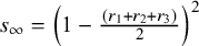
Remark 6.4. While proving Theorem 6.1, we in fact computed the F-signature function $\psi _p$
itself for certain values of t. For polynomial f and parameters
$\psi _p$
itself for certain values of t. For polynomial f and parameters $a\geq b\geq c$
as in the theorem statement, and for any integer r and prime p with
$a\geq b\geq c$
as in the theorem statement, and for any integer r and prime p with $0<\frac {r}{p}< \min \{\frac {1}{a},\frac {2}{a+b+c}\}$
, we have
$0<\frac {r}{p}< \min \{\frac {1}{a},\frac {2}{a+b+c}\}$
, we have
 $$\begin{align*}\psi_p\left(\frac{r}{p}\right) = \begin{cases} 1 - (a+b+c)\frac{r}{p}+a(b+c)\frac{r^2}{p^2} & a\geq b+c \\ 1 - (a+b+c)\frac{r}{p} +\frac{1}{p^2}\lfloor \frac{(a+b+c)^2r^2}{4}\rfloor & a<b+c \end{cases}. \end{align*}$$
Remark 6.5. The F-signature functions $\psi _p (t)$
from Theorem 6.1 do not always stabilize to the limit
$\psi _p (t)$
from Theorem 6.1 do not always stabilize to the limit $\psi (t)$
for large values of p on any sub-interval of
$\psi (t)$
for large values of p on any sub-interval of $(0,1)$
. Indeed, take
$(0,1)$
. Indeed, take $a,b,c$
to be positive integers such that
$a,b,c$
to be positive integers such that $a < b+c$
and
$a < b+c$
and $a + b + c$
is odd. Then, in any sub-interval
$a + b + c$
is odd. Then, in any sub-interval $\emptyset \neq I \subset (0,1)$
, we can find primes
$\emptyset \neq I \subset (0,1)$
, we can find primes $p \gg 0 $
and odd integers
$p \gg 0 $
and odd integers $r_p$
such that
$r_p$
such that $\frac {r_p}{p} \in I$
, so that by comparing Theorems 6.4 and 6.1, we see that
$\frac {r_p}{p} \in I$
, so that by comparing Theorems 6.4 and 6.1, we see that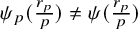 $\psi _p (\frac {r_p}{p}) \neq \psi (\frac {r_p}{p})$
. We do not know if
$\psi _p (\frac {r_p}{p}) \neq \psi (\frac {r_p}{p})$
. We do not know if $\psi _p (t)$
stabilizes for
$\psi _p (t)$
stabilizes for $p \gg 0$
for a fixed t, but we expect the answer to be negative. See [Reference Caminata, Shideler, Tucker and Zerman9, Theorem 7.1] for a similar phenomenon.
$p \gg 0$
for a fixed t, but we expect the answer to be negative. See [Reference Caminata, Shideler, Tucker and Zerman9, Theorem 7.1] for a similar phenomenon.
Theorem 6.6. Let $g = x^a y^b (x^u + y^v) ^c $
for non-negative integers a, b, c, u, and v. Assume that u, v, and c are positive. We consider g as a polynomial in
$g = x^a y^b (x^u + y^v) ^c $
for non-negative integers a, b, c, u, and v. Assume that u, v, and c are positive. We consider g as a polynomial in ${\mathbb {Z}}[x,y]$
, so that we may consider the reduction of g to characteristic
${\mathbb {Z}}[x,y]$
, so that we may consider the reduction of g to characteristic $p>0$
for each prime p. Set
$p>0$
for each prime p. Set $\lambda _0 = \frac {\frac {1}{u} + \frac {1}{v}}{\frac {a}{u} + \frac {b}{v} + c}$
, and
$\lambda _0 = \frac {\frac {1}{u} + \frac {1}{v}}{\frac {a}{u} + \frac {b}{v} + c}$
, and $\lambda = \min \{\frac {1}{a}, \frac {1}{b}, \frac {1}{c}, \lambda _0 \}$
. Let
$\lambda = \min \{\frac {1}{a}, \frac {1}{b}, \frac {1}{c}, \lambda _0 \}$
. Let $\psi (t)$
be the limit F-signature function of g, which is defined by
$\psi (t)$
be the limit F-signature function of g, which is defined by
 $$\begin{align*}\psi(t):= \lim_{p \to \infty} s_p(\mathbb{F}_p[x,y], g^t). \end{align*}$$
Then, for $t < \lambda $
,
$t < \lambda $
, $\psi (t)$
is given by the following formula:
$\psi (t)$
is given by the following formula:
-
1. If
$tav +u \geq tbu+v+cuvt$
, then
$\psi (t) = ( 1 -at) (1- (b +cv)t)$
. -
2. If
$tbu +v \geq tav+u+cuvt$
, then
$\psi (t) = (1-bt) (1 - (a +cu)t)$
. -
3. If
$tcuv + u + v \geq tav + tbu +2uv $
, then
$\psi (t) = (1-ct) (v(1-at) + u (1-bt) -uv)$
. -
4. Otherwise,
$\psi (t) = \frac {1}{4uv} (u+v - t(av + bu+ cuv))^2$
.







Remark 6.7. If instead any one of u, v, or c is zero, then the F-signature function of the pair $(\mathbb {F}_p [x,y]_{(x,y)},\, g = x^a y^b (x^u + y^v)^c)$
reduces to the monomial case from Theorem 6.2. This is because in that case
$(\mathbb {F}_p [x,y]_{(x,y)},\, g = x^a y^b (x^u + y^v)^c)$
reduces to the monomial case from Theorem 6.2. This is because in that case $(x^u + y^v)^c$
is a unit in the localization
$(x^u + y^v)^c$
is a unit in the localization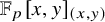 $\mathbb {F}_p [x,y]_{(x,y)}$
, so the divisor defined by g is the same as the divisor defined by
$\mathbb {F}_p [x,y]_{(x,y)}$
, so the divisor defined by g is the same as the divisor defined by $x^a y^b$
, and consequently, the F-signature functions are the same.
$x^a y^b$
, and consequently, the F-signature functions are the same.
Before proving Theorem 6.6, we prove some useful lemmas, the first of which will allow us to reduce to the case when $u=v=1$
.
$u=v=1$
.
Lemma 6.8. Fix non-negative integers a, b, c, u, and v, and fix a prime $p> uv$
. Consider the polynomials
$p> uv$
. Consider the polynomials
 $$\begin{align*}g=x^ay^b(x^u+y^v)^c, \quad \widetilde{g} = x^{va} (x + y)^{cuv}y^{ub}, \quad\textrm{and}\quad g_0 = x^{v(u-1)} y^{u (v-1)}.\end{align*}$$
Then, for any $t>0$
, we have
$t>0$
, we have
 $$\begin{align*}s_p(\mathbb{F}_p [x,y], g^t) = uv \, s_p(\mathbb{F}_p [x,y], \, g_0 ^{\frac{1}{uv}} \, \widetilde{g}^{\frac{t}{uv}}).\end{align*}$$
Proof. Let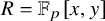 $R = \mathbb {F}_p [x,y]$
and define
$R = \mathbb {F}_p [x,y]$
and define
 $$\begin{align*}S = R[x', y']/ ((x')^u- x , (y')^v - y). \end{align*}$$
Note that S is isomorphic to the polynomial ring generated by $x'$
and
$x'$
and $y'$
(over
$y'$
(over $\mathbb {F}_p$
), and R can be identified with the subring of S generated by
$\mathbb {F}_p$
), and R can be identified with the subring of S generated by $x = (x')^{u}$
and
$x = (x')^{u}$
and $y = (y')^v$
. Denoting
$y = (y')^v$
. Denoting $X = \operatorname {\mathrm {{Spec}}}(R)$
and
$X = \operatorname {\mathrm {{Spec}}}(R)$
and $Y = \operatorname {\mathrm {{Spec}}}(S)$
and
$Y = \operatorname {\mathrm {{Spec}}}(S)$
and $\pi $
to be the induced map
$\pi $
to be the induced map $\pi : Y \to X$
, we have that
$\pi : Y \to X$
, we have that $\pi $
is a finite separable map of degree
$\pi $
is a finite separable map of degree $uv$
(it is separable since
$uv$
(it is separable since $p> uv$
). Note that the ramification divisor
$p> uv$
). Note that the ramification divisor $\text {Ram}_\pi $
is given by
$\text {Ram}_\pi $
is given by
 $$\begin{align*}\text{Ram}_\pi = (u-1) \operatorname{\mathrm{div}}(x') + (v-1)\operatorname{\mathrm{div}}(y'). \end{align*}$$
Now, we consider the $\mathbb {Q}$
-divisor
$\mathbb {Q}$
-divisor
 $$\begin{align*}\Delta_X = \operatorname{\mathrm{div}} (g_0 ^{\frac{1}{uv}} \widetilde{g}^{\frac{t}{uv}}) = \frac{ta + (u-1)}{u} \operatorname{\mathrm{div}}(x) + ct \, \operatorname{\mathrm{div}}(x + y) + \frac{tb + (v-1)}{v} \operatorname{\mathrm{div}}(y).\end{align*}$$
Then, using the fact that $\pi ^* (\operatorname {\mathrm {div}}(x)) = u \operatorname {\mathrm {div}} (x')$
,
$\pi ^* (\operatorname {\mathrm {div}}(x)) = u \operatorname {\mathrm {div}} (x')$
, $\pi ^* (\operatorname {\mathrm {div}}(y)) = v \operatorname {\mathrm {div}} (y')$
, and
$\pi ^* (\operatorname {\mathrm {div}}(y)) = v \operatorname {\mathrm {div}} (y')$
, and $\pi ^* (\operatorname {\mathrm {div}}(x + y)) = \operatorname {\mathrm {div}}((x')^{u} + (y')^{v})$
, we compute
$\pi ^* (\operatorname {\mathrm {div}}(x + y)) = \operatorname {\mathrm {div}}((x')^{u} + (y')^{v})$
, we compute
 $$\begin{align*}\Delta_Y = \pi^* \Delta_X - \text{Ram}_\pi = ta \operatorname{\mathrm{div}}(x') + ct \operatorname{\mathrm{div}}((x')^u + (y')^v) + tb\operatorname{\mathrm{div}}(y') = \operatorname{\mathrm{div}} (g^t), \end{align*}$$
where we view in g as a polynomial in $x'$
and
$x'$
and $y'$
. Note that
$y'$
. Note that $\Delta _Y$
is effective. Furthermore, since
$\Delta _Y$
is effective. Furthermore, since $R \to S$
is a finite separable extension of normal domains and the degree is coprime to p, and since the corresponding map on the residue fields is an isomorphism, the number of
$R \to S$
is a finite separable extension of normal domains and the degree is coprime to p, and since the corresponding map on the residue fields is an isomorphism, the number of $\text {Tr}$
-summands of S over R is equal to
$\text {Tr}$
-summands of S over R is equal to $1$
by [Reference Carvajal-Rojas, Schwede and Tucker11, Lemma 2.13]. Now, by applying [Reference Carvajal-Rojas, Schwede and Tucker11, Theorem 4.4], we conclude that
$1$
by [Reference Carvajal-Rojas, Schwede and Tucker11, Lemma 2.13]. Now, by applying [Reference Carvajal-Rojas, Schwede and Tucker11, Theorem 4.4], we conclude that
 $$\begin{align*}s_p (Y, \Delta_Y) = uv \, s_p (X, \Delta_X) \end{align*}$$
as required.
Lemma 6.9. Assume $a,b$
are non-negative integers and
$a,b$
are non-negative integers and $c,u,v$
are positive integers. The log canonical threshold of
$c,u,v$
are positive integers. The log canonical threshold of $g = x^a y^b (x^u + y^v) ^c$
is equal to
$g = x^a y^b (x^u + y^v) ^c$
is equal to
 $$\begin{align*}\lambda = \min \left\{\frac{1}{a}, \frac{1}{b}, \frac{1}{c}, \lambda_0 \right\}, \end{align*}$$
where $\lambda _0 = \frac {\frac {1}{u} + \frac {1}{v}}{\frac {a}{u} + \frac {b}{v} + c}$
.
$\lambda _0 = \frac {\frac {1}{u} + \frac {1}{v}}{\frac {a}{u} + \frac {b}{v} + c}$
.
Proof. We provide a proof using finite covers similar to the proof of Theorem 6.8. Let $g_0 = x^{u (v-1)} y ^{v (u -1)}$
and let
$g_0 = x^{u (v-1)} y ^{v (u -1)}$
and let $\tilde g = x^{va} (x+y) ^{cuv} y^{ub}$
. Then, the pair
$\tilde g = x^{va} (x+y) ^{cuv} y^{ub}$
. Then, the pair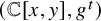 $(\mathbb {C}[x,y], g^{t})$
is KLT if and only if
$(\mathbb {C}[x,y], g^{t})$
is KLT if and only if $(\mathbb {C}[x,y], g_0 ^{1/uv} \tilde g ^{t/uv})$
is KLT. This follows from the exact same computation as in Theorem 6.8 and using the transformation rule for multiplier ideals under finite covers [Reference Blickle, Schwede and Tucker8, Theorem 8.1]. Alternatively, we could also use reduction modulo p to prove the statement for F-regularity first, in which case it follows from Theorem 6.8 and the fact that the F-signature is positive if and only if the pair is strongly F-regular [Reference Blickle, Schwede and Tucker6, Theorem 3.18]. In any case, this shows that the log canonical threshold is given by the supremum
$(\mathbb {C}[x,y], g_0 ^{1/uv} \tilde g ^{t/uv})$
is KLT. This follows from the exact same computation as in Theorem 6.8 and using the transformation rule for multiplier ideals under finite covers [Reference Blickle, Schwede and Tucker8, Theorem 8.1]. Alternatively, we could also use reduction modulo p to prove the statement for F-regularity first, in which case it follows from Theorem 6.8 and the fact that the F-signature is positive if and only if the pair is strongly F-regular [Reference Blickle, Schwede and Tucker6, Theorem 3.18]. In any case, this shows that the log canonical threshold is given by the supremum
 $$\begin{align*}\sup \left\{ t \geq 0 \, | \, \max \{\frac{u-1 + at}{u}, \frac{v-1 + bt}{v}, ct, \frac{\frac{u - 1 + at}{u} + \frac{v -1 + bt}{v} + ct} {2} \} \leq 1 \right\} .\end{align*}$$
One checks that the four possible values for $\lambda $
as proposed correspond to the four values in the above maximum being equal to
$\lambda $
as proposed correspond to the four values in the above maximum being equal to $1$
. This shows that
$1$
. This shows that $\lambda $
is equal to the supremum as required.
$\lambda $
is equal to the supremum as required.
Proof of Theorem 6.6
First, we note that the proposed formula for $\psi (t)$
in the theorem defines a continuous, non-increasing function. Thus, by Theorem 2.5, it is sufficient to show that
$\psi (t)$
in the theorem defines a continuous, non-increasing function. Thus, by Theorem 2.5, it is sufficient to show that $\psi (t)$
matches with the limit F-signature function for rational values of t. Therefore, we may assume that t is rational. From Theorem 6.8, for each
$\psi (t)$
matches with the limit F-signature function for rational values of t. Therefore, we may assume that t is rational. From Theorem 6.8, for each $p> uv$
and
$p> uv$
and $t \geq 0$
, we have the transformation rule
$t \geq 0$
, we have the transformation rule
 $$\begin{align*}s_p(\mathbb{F}_p[x,y], g^t) = uv \, s_p(\mathbb{F}_p[x,y], x^{\frac{at+u-1}{u}} y^{\frac{bt+v-1}{v}} (x+y)^{ct} ). \end{align*}$$
Then, for rational number $t < \lambda $
, we may compute the limit F-signature
$t < \lambda $
, we may compute the limit F-signature $\psi (t)$
using Theorem 6.1 for the right-hand side (see Theorem 6.3) and we obtain the following cases:
$\psi (t)$
using Theorem 6.1 for the right-hand side (see Theorem 6.3) and we obtain the following cases:
-
1. If
$\frac {at + u-1}{u} \geq \frac {bt + v-1}{v} + ct $
: In this case, we have
$$\begin{align*}\psi(t) = uv \, \left(1 - \frac{at + u-1}{u}\right) \left(1 - \left(\frac{bt + v-1}{v} + ct\right)\right) = (1 - at)(1 - (b+cv)t). \end{align*}$$
Note that by rearranging the inequality
$\frac {at + u-1}{u} \geq \frac {bt + v-1}{v} + ct $
, it is equivalent to
$tav + u \geq tbu + v + cuvt$
. -
2. If
$\frac {bt + v-1}{v} \geq \frac {at + u-1}{u} + ct $
: By symmetry between
$(a,u)$
and
$(b,v)$
, in this case, we have
$$\begin{align*}\psi(t) = (1 - bt) (1 - (a+cu)t). \end{align*}$$
-
3. If
$ct \geq \frac {at + u-1}{u} + \frac {bt + v-1}{v} $
: In this case, we have
$$\begin{align*}\psi(t) = uv \, (1 - ct) \left(1 - \left(\frac{at + u-1}{u} + \frac{bt + v-1}{v} \right)\right) = ( 1- ct) (u+v - avt - but - uv), \end{align*}$$
and the last term simplifies to
$v(1-at) + u (1-bt) - uv$
. We also note that the condition
$ct \geq \frac {at + u-1}{u} + \frac {bt + v-1}{v} $
can be rearranged to
$tcuv + u+v \geq tav + tbu + 2uv$
. -
4. Otherwise: Lastly, we note that in the complementary cases, the formula in Theorem 6.3 is symmetric in
$r_1$
,
$r_2$
, and
$r_3$
so the relative order does not matter. Therefore, in the complementary cases, we have
$$\begin{align*}\psi(t) = uv \, \left(1 - \frac{1}{2}\left(\frac{u+at -1}{u} + \frac{bt+v - 1}{v} + ct\right)\right)^2 = \frac{1}{4uv}(u+v - (atv + btu+ ctuv))^2\end{align*}$$
as desired.














7. Relation to the normalized volume
In this section, we provide a geometric interpretation for the formula of the limit F-signature obtained in Theorem 6.6 in terms of an invariant of complex KLT singularities called the normalized volume. Recall that KLT singularities are related to strongly F-regular singularities via reduction to characteristic p [Reference Hara14], [Reference Hara and Yoshida15], [Reference Mehta and Srinivas25], [Reference Smith34], [Reference Takagi36]. See [Reference Schwede and Tucker33, Section 4] for an introduction and additional references. More recently, the normalized volume of KLT singularities was introduced by Li in relation to K-stability and the existence of Kähler–Einstein metrics on Fano varieties. We begin by reviewing the definition of the normalized volume.
Definition 7.1. [Reference Li19] Let $x \in (X, \Delta )$
be a local KLT pair over
$x \in (X, \Delta )$
be a local KLT pair over $\mathbb {C}$
at a closed point
$\mathbb {C}$
at a closed point $x \in X$
. Then, the normalized volume
$x \in X$
. Then, the normalized volume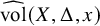 ${\widehat {\rm vol}} (X, \Delta , x)$
is defined as
${\widehat {\rm vol}} (X, \Delta , x)$
is defined as
 $$\begin{align*}{\widehat{\rm vol}} (X, \Delta, x) = \inf \{ A_{X, \Delta} (v) ^n \, \text{vol}(v) \, | \, v \text{ divisorial valuation centered at } x \}. \end{align*}$$
Here, n denotes the dimension of X and $A_{X, \Delta }$
denotes the log discrepancy of a divisorial valuation with respect to
$A_{X, \Delta }$
denotes the log discrepancy of a divisorial valuation with respect to $(X, \Delta )$
.
$(X, \Delta )$
.
Let $f = x^a \, y^b \, (x+y) ^c$
for non-negative integers
$f = x^a \, y^b \, (x+y) ^c$
for non-negative integers $a \geq b \geq c$
and
$a \geq b \geq c$
and $t \geq 0$
be a rational parameter. For pairs considered in this article, namely, of the form
$t \geq 0$
be a rational parameter. For pairs considered in this article, namely, of the form $(X = \operatorname {\mathrm {{Spec}}}(\mathbb {C}[x,y]), \Delta = \operatorname {\mathrm {div}} (f^t)) $
, the normalized volume of
$(X = \operatorname {\mathrm {{Spec}}}(\mathbb {C}[x,y]), \Delta = \operatorname {\mathrm {div}} (f^t)) $
, the normalized volume of $(X, \Delta )$
was computed by Li in [Reference Li20, Section 4.1]. In our notation, the formula from [Reference Li20] is written as:
$(X, \Delta )$
was computed by Li in [Reference Li20, Section 4.1]. In our notation, the formula from [Reference Li20] is written as:
-
1. If
$t \geq \min \{ \frac {1}{a}, \frac {2}{a+b+c} \}$
, then
$ {\widehat {\rm vol}} (X, \Delta ) = 0 $
. -
2. If
$t< \min \{ \frac {1}{a}, \frac {2}{a+b+c} \}$
and
$a \geq b +c$
, then
${\widehat {\rm vol}} (X, \Delta ) = 4 \, (1 - (b+c)t) (1 - at)$
. -
3. If
$t < \min \{ \frac {1}{a}, \frac {2}{a+b+c} \}$
and
$a < b +c$
, then
${\widehat {\rm vol}} (X, \Delta ) = (2 - (a+b+c)t)^2.$

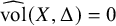






By direct inspection with the formula obtained in Theorem 6.1, we obtain the following relation between the normalized volume and the limit F-signature.
Corollary 7.2. Let $(X, \Delta ) = (\operatorname {\mathrm {{Spec}}}({\mathbb {Z}}[x,y]), \operatorname {\mathrm {div}} (f^t))$
, where
$(X, \Delta ) = (\operatorname {\mathrm {{Spec}}}({\mathbb {Z}}[x,y]), \operatorname {\mathrm {div}} (f^t))$
, where $f= x^a \, y^b \, (x+y) ^c$
and
$f= x^a \, y^b \, (x+y) ^c$
and $t \geq 0$
is a rational parameter. Then, we have
$t \geq 0$
is a rational parameter. Then, we have
 $$ \begin{align} \frac{{\widehat{\rm vol}}(X_{\mathbb{C}}, \Delta_{\mathbb{C}})}{4} = \lim_{p \to \infty} s_p (X_p, \Delta_p), \end{align} $$
where $X_{\mathbb {C}}, X_p$
denote the base changes of X to
$X_{\mathbb {C}}, X_p$
denote the base changes of X to $\mathbb {C}$
and to
$\mathbb {C}$
and to $\mathbb {F}_p$
, respectively (and similarly for
$\mathbb {F}_p$
, respectively (and similarly for $\Delta $
).
$\Delta $
).
We thank Yuchen Liu for pointing us to this connection.
Remark 7.3. The F-signature and the normalized volume satisfy many analogous properties (see [Reference Carvajal-Rojas, Schwede and Tucker11], [Reference Ma, Polstra, Schwede and Tucker24], [Reference Taylor38]) and are expected to be related via the reduction modulo p process as evidenced in Theorem 7.2 (see [Reference Li, Liu and Xu21, Section 6.3.1]).
We also note that Equation (7.2.1) holds for all two-dimensional KLT singularities $(X, x)$
, when
$(X, x)$
, when $\Delta = 0$
, since they are quotient singularities. This leads to the following natural prediction for the values of the limit F-signature function of homogeneous polynomials in two variables in terms of the normalized volume as computed in [Reference Li20, Section 4.1].
$\Delta = 0$
, since they are quotient singularities. This leads to the following natural prediction for the values of the limit F-signature function of homogeneous polynomials in two variables in terms of the normalized volume as computed in [Reference Li20, Section 4.1].
Question 7.4. Does Equation (7.2.1) hold for all homogeneous polynomials $f \in \mathbb {C}[x,y]$
and all rational numbers
$f \in \mathbb {C}[x,y]$
and all rational numbers $t \geq 0$
?
$t \geq 0$
?
Acknowledgements
The authors thank Nasrin Altafi, Jenny Kenkel, Yuchen Liu, Alexandra Seceleanu, and Karen E. Smith for insightful conversations, as well as Michael Perlman, whose undergraduate honors thesis contained a number of preliminary related investigations. The authors thank the referee for valuable comments and for pointing out the reference [Reference Han13] and other useful comments. The authors thank the hospitality of the Simons-Laufer Mathematical Sciences Institute (formerly the Mathematical Sciences Research Institute, and which is supported by the National Science Foundation Grant No. DMS-1928930 and the Alfred P. Sloan Foundation under grant G-2021-16778), where parts of the research were carried out in Berkeley, California, during the Spring 2024 semester.
A.B. was supported in part by NSF grants DMS no. 1840234 and no. 2101075 and by NSF Postdoctoral Fellowship no. 2402293. S.P. was supported in part by NSF grants no. 1952399, no. 1801697, and no. 2101075. I.C. was supported in part by the NSF Grant DMS no. 2200684. K.T. was supported in part by NSF Grant DMS no. 2200716 and no. 2501904.


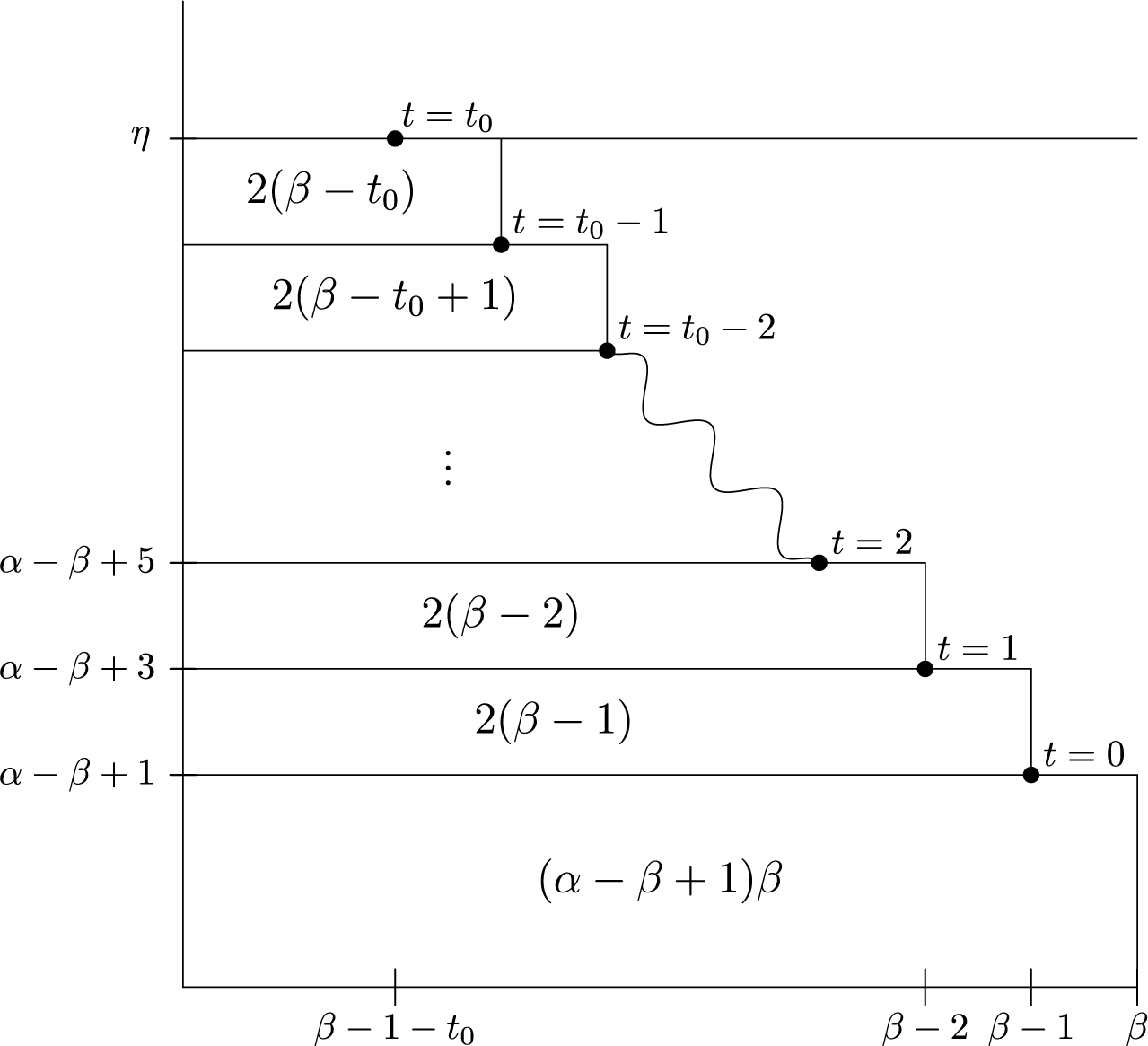


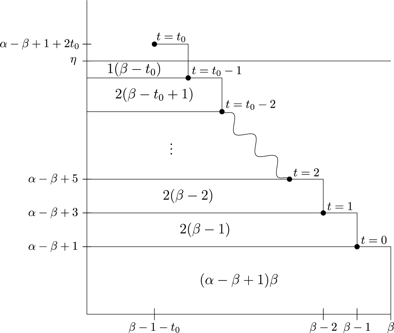


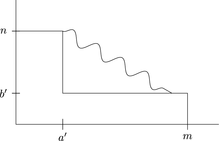


 Open access

