2.1. Electrical conductivity

EM mapping of groundwater exploits the differences in electrical conductivity between pore fluids and the surrounding sediments and bedrock. A key motivating factor for using EM in a glaciated environment is the large difference in conductivity between ice and groundwater. Low-impurity ice has a conductivity that is primarily governed by the slow movement of protonic point defects, resulting in a resistivity (the inverse of conductivity) of ~0.4 × 10⁵ Ω-m at ~2°C, which increases to 4 × 10⁵ Ω-m at −58°C (Petrenko and Whitworth, Reference Petrenko and Whitworth2002; Kulessa, Reference Kulessa2007). The high resistivity of ice is juxtaposed with the significantly lower resistivity of groundwater, where electrical conduction is primarily an electrolytic process dominated by the concentration and mobility of ions (Kirsch, Reference Kirsch2006). The resistivity of water strongly decreases with salinity (Perkin and Lewis, Reference Perkin and Lewis1980). Pure deionized fresh water has a resistivity of ~10⁴ Ω-m, but the addition even small amounts of ions will greatly decrease this value. For example, water with practical salinity <0.5 is considered to be fresh, yet has a resistivity as low as 20 Ω-m (Perkin and Lewis, Reference Perkin and Lewis1980), over 500 times more conductive than pure fresh water (Fig. 2). Seawater at ~1°C is ~0.3 Ω-m, and hypersaline fluids are even less resistive.

Fig. 2. Bulk electrical resistivity of sediments shown as a function of pore fluid salinity and sediment porosity. Bulk resistivity was computed using Archie's Law with exponent m = 1.5 and temperature 0°C. The resistivity of pore-water (100% porosity) is from the Practical Salinity Scale 1978 (Perkin and Lewis, Reference Perkin and Lewis1980). Red dots show direct water measurements from West Lake Bonney (WLB) at 5 and 38 m depth (Spigel and Priscu, Reference Spigel and Priscu1996) and Casey Station (CS) jökulhlaup outflow (Goodwin, Reference Goodwin1988). The dashed green line shows pore-water resistivity at Subglacial Lake Whillans (SLW) rapidly decreasing from the lake bottom to 0.4 m into the sediments (Christner and others, Reference Christner2014; Michaud and others, Reference Michaud2016). For reference, the resistivity of ice greatly exceeds 10⁴ Ω-m.

Because of its dependence on ionic content, the bulk resistivity of groundwater reflects its provenance and residence time: newly formed fresh water produced by local basal melting of clean ice will have low ion concentrations and hence high resistivity, while older mixed waters may exhibit lower resistivity due to increased ionic content from geochemical dissolution of surrounding sediments or bedrock as well as from mixing with existing saline pore fluids. Indeed, this has been the case with groundwater samples from Antartica (Fig. 2). At Subglacial Lake Whillans (SLW), located beneath Whillans Ice Stream, West Antarctica, water salinity exhibits a steep gradient in depth from a value slightly more saline than fresh water at the lake's top to brackish water less than a meter below (Michaud and others, Reference Michaud2016). Geochemical analysis of these samples indicates only up to a 6% contribution from ancient seawater, and that most of the solutes arise from crustal silicate weathering from a more concentrated source at depth (Michaud and others, Reference Michaud2016). Samples from West Lake Bonney, a saline lake with a permanently frozen cover in Taylor Valley, show salinities ranging from brackish at shallow depths to hypersaline brines at 38 m depth (Spigel and Priscu, Reference Spigel and Priscu1996). Sampling of a jökulhlaup near Casey Station, Law Dome, revealed nearly fresh outflow with low resistivity and high solute content, suggesting it had been squeezed through subglacial sediments for a considerable time period (Goodwin, Reference Goodwin1988).

The bulk resistivity of water-saturated sediments, till and bedrock can be estimated using Archie's Law, an empirical formula found to work well for porous sediments (Archie, Reference Archie1942) and fractured bedrock (Brace and Orange, Reference Brace and Orange1968). In Figure 2, we also show the bulk resistivity for variable porosity sediments that are saturated with water of variable salinity. Resistivity decreases as porosity and salinity increase. For the minimum 1% porosity considered, the bulk resistivity is much lower than that of ice, even for salinity values considered to be fresh.

Remote characterization of the subglacial resistivity structure can therefore provide a fundamental constraint on the fluid content of the subglacial environment; for example, a wet subglacial lake or sediment package will be relatively conductive, whereas dry or frozen ground will be significantly more resistive. In addition to detecting free water in lakes beneath ice, EM data could be used to reveal groundwater systems in deeper underlying sediments and fractured bedrock, which likely has important consequences for subglacial biology and geochemical cycles (Wadham and others, Reference Wadham2012, Reference Wadham2013; Vick-Majors, Reference Vick-Majors2016), and may represent a volumetrically larger component of water than the thin distributed sheets or channelized streams at the base of the ice (Christoffersen and others, Reference Christoffersen, Bougamont, Carter, Fricker and Tulaczyk2014). Little is currently known about the deeper hydrology due to the limitations of existing geophysical data and a lack of deep borehole data in Antarctica.

2.2. EM imaging methods

EM geophysical techniques use low-frequency (<10 kHz) EM induction that is governed by a vector diffusion equation (Ward and Hohmann, Reference Ward, Hohmann and Nabighian1987). They have been well developed for tectonic, mineral, hydrocarbon and groundwater exploration (Nabighian, Reference Nabighian1987; Kirsch, Reference Kirsch2006; Chave and Jones, Reference Chave and Jones2012). Depending on the particular technique, EM data can be preferentially sensitive to conductive features such as zones with high groundwater content, or sensitive to resistive features such as hydrocarbon reservoirs.

Because both the frequency range of EM measurements and the resistivity of the target geology can vary by orders of magnitude, the depth sensitivity of EM data can vary greatly. A measure of this is provided by the EM skin depth z _s, which is the e-folding distance of the induced field in a uniform conductor. The skin depth depends on the resistivity ρ and linear frequency f according to:

(1) $$z_{\rm s} \approx 500\sqrt {\rho /f} \;{\rm m}$$

(Ward and Hohmann, Reference Ward, Hohmann and Nabighian1987). For a given resistivity, the skin depth relation shows that high-frequency energy attenuates more rapidly and is sensitive to shallow structure, while low-frequency energy can penetrate more deeply. For subglacial EM imaging, high frequencies can constrain conductive water at the glacier bed but will have attenuated too much to be sensitive to deeper structure, while much lower frequencies with longer skin depths can constrain the deeper bed and basement conductivity. For example, consider a 3 Ω-m water body at the glacier bed. The skin depth at 10 000 Hz is only 9 m, while at 1 Hz, the skin depth is ~900 m. This is contrasted by the significantly higher frequencies of radar data (>10 MHz), which can only detect the top of a water layer since rapid attenuation within the layer limits deeper sensitivity (Schroeder and others, Reference Schroeder, Blankenship, Raney and Grima2015), except in the limiting case where the water is fresh enough to have a very high resistivity and is ~<10 m thick (Gorman and Siegert, Reference Gorman and Siegert1999; Dowdeswell and Evans, Reference Dowdeswell and Evans2004). Active-source seismic data, which are governed by the wave equation, can reveal high-resolution images of subglacial geologic boundaries (Blankenship and others, Reference Blankenship, Bentley, Rooney and Alley1986; Smith, Reference Smith1997), but are much less sensitive to water content than EM data.

EM methods can be broadly divided into the passive magnetotelluric (MT) method and various controlled-source EM methods (Fig. 1). The MT method uses variations in naturally occurring low-frequency electric and magnetic fields to probe the electrical-conductivity structure of, typically, the crust and mantle (Chave and Jones, Reference Chave and Jones2012). The source field arises from interactions of charged particles in the solar wind with the conductive ionosphere, producing stochastic time-varying currents that emanate plane-wave like pulsations down through the resistive lower atmosphere. At high frequencies (>1 Hz), additional source energy arises from the global distribution of lightning strikes resonating in the atmospheric cavity. This incident energy diffuses into the conducting Earth, inducing secondary electric and magnetic fields that depend on the conductivity structure.

MT data consist of time series measurements of the horizontal electric and magnetic fields at the surface, which are used to estimate a complex frequency-dependent impedance tensor that relates the electric- and magnetic-field vectors. Impedance responses measured at a series of MT stations are typically inverted using a non-linear optimization approach that solves for a conductivity model that fits the observed data. Because of the skin-depth dependence of EM fields on the frequency and resistivity, MT measurements can be used to image features on dramatically different depth scales, depending on the electrical structure and length of data acquisition. For example, recordings of weeks to months over the resistive oceanic lithosphere have been used to study partial melts in the mantle (Baba and others, Reference Baba, Chave, Evans, Hirth and Mackie2006; Key and others, Reference Key, Constable, Liu and Pommier2013; Naif and others, Reference Naif, Key, Constable and Evans2013), whereas high-frequency recordings of a day or less duration can be used to study groundwater in the shallow crust (Unsworth and others, Reference Unsworth, Egbert and Booker1999; Garcia and Jones, Reference Garcia and Jones2010).

Controlled-source EM soundings use a transmitter to generate the EM field. The transmitter can take the form of either a grounded dipole or a large ungrounded loop. From a theoretical point of view, the grounded dipole source is preferred since it produces both transverse electric (TE) and transverse magnetic (TM) polarization modes of the EM field, and thus has a richer structural sensitivity than a loop source, which only generates the TE mode (Chave and Cox, Reference Chave and Cox1982; Ward and Hohmann, Reference Ward, Hohmann and Nabighian1987). However, since the signal-to-noise ratio of EM data is directly proportional to the current in the transmitter wire, the large loop method is often preferred in areas where high ground contact resistance (e.g. ice, bedrock, or extremely dry cover) severely limits the amount of current that can be injected with a grounded dipole. Further, loop sources can also be mobilized, for example, for highly efficient airborne EM surveys (Christiansen and others, Reference Christiansen, Auken and Sørensen2006). Because they only generate the TE mode, loop sources create EM fields that are preferentially sensitive to conductive features.

The loop source creates a large magnetic dipole field that is pulsed in time, inducing eddy currents in the subsurface that in turn create secondary magnetic fields. The resulting total magnetic field at the surface is measured at one or more receiver stations. Since this controlled-source EM method can generate a much stronger source field than the natural MT fields and since electric fields do not need to be measured, surveys can often be acquired rapidly. Data acquisition can use a time domain or frequency domain approach. In the time-domain approach known as the transient EM (TEM) method, the transmitter current is rapidly turned off and the resulting transient pulse is recorded (Christiansen and others, Reference Christiansen, Auken and Sørensen2006). For TEM soundings, the response at early times gives shallow sensitivity, while the response at late times gives deeper depth sensitivity. Conversely, measurements can be made in the frequency domain using a periodic transmitter waveform with the EM responses computed at the various waveform harmonics. Here, we will refer to frequency domain EM as FDEM.

One of the fundamental differences between TEM and FDEM is the ability to record measurements coincident with the loop source. Close to the source, the primary magnetic field generated by the loop can be many orders of magnitude larger than the secondary field. Thus, FDEM measurements, which record the superposition of both fields, can have low sensitivity to the secondary field close to the source. Conversely, TEM measurements can be made close to the source since the primary field travels through the air and rapidly propagates away during early times after the current is turned off, whereas the secondary-field transient arising from the ground response travels more slowly and appears at later times. Thus, TEM measurements tend to be made with receivers located within or next to the loop source, whereas FDEM measurements tend to be made with receivers at a distance from the source where the induced secondary-field strength is of similar order to the primary field.

2.3. Previous EM surveys in Antarctica

Early MT surveys in Antarctica include low-frequency measurements of the telluric current at Vostok Station (Hessler and Jacobs, Reference Hessler and Jacobs1966) and reports mentioning MT data collected at Dome C (Bentley and others, Reference Bentley, Jezek, Blankenship, Lovell and Albert1979; Shabtaie and others, Reference Shabtaie, Bentley, Blankenship, Lovell and Gassett1980). Beblo and Liebig (Reference Beblo and Liebig1990) present the first quantitative analysis of Antarctic MT data, describing a suite of four stations collected on Priestly Glacier, North Victoria Land, with encouraging results for investigating sub-ice sedimentary basins. More recent studies have concentrated on using low-frequency MT data to study deep crustal and upper mantle tectonics (Wannamaker and others, Reference Wannamaker, Stodt and Olsen1996, Reference Wannamaker, Stodt, Pellerin, Olsen and Hall2004, Reference Wannamaker2012; Peacock and Selway, Reference Peacock and Selway2016). Although theoretical considerations suggest that departures from the MT plane-wave source-field assumption may be prevalent at the poles due to the presence of the polar atmospheric electrojets (Pirjola, Reference Pirjola1998), Beblo and Liebig (Reference Beblo and Liebig1990) showed that MT impedance responses from different time segments remain stationary despite clear variations in source strength associated with the electrojet. This conclusion is also supported by the lack of source-effect complications in more recent datasets (Wannamaker and others, Reference Wannamaker, Stodt and Olsen1996, Reference Wannamaker, Stodt, Pellerin, Olsen and Hall2004; Peacock and Selway, Reference Peacock and Selway2016).

The use of controlled-source EM methods in Antarctica has been very limited. Ruotoistenmäki and Lehtimäki (Reference Ruotoistenmäki and Lehtimäki1997) report on a pioneering use of FDEM to map saline brines beneath continental ice and permafrost in western Dronning Maud Land, where they mapped the depth to a subglacial conductive layer along a 35 km transect. Their multifrequency system collected data at 2–20 000 Hz with source-receiver offsets up to 1500 m. Where the ice was <650 m thick, their system found 20–500 Ω-m subglacial conductors that they attributed to saline brines. A more recent exception is the groundbreaking use of helicopter-based TEM surveying carried out in 2011–2012 to map shallow groundwater in the McMurdo Dry Valleys, East Antarctica. This dataset has revealed laterally extensive zones of conductive groundwater throughout the Dry Valleys, including a confined aquifer beneath Lake Vida (Dugan and others, Reference Dugan2015) and conductive groundwater confined beneath the lower extent of Taylor Glacier, which may extend far upstream (Foley and others, Reference Foley2015; Mikucki and others, Reference Mikucki2015). This recent EM-based discovery of extensive groundwater, despite an abundance of previous non-EM studies in this region, illustrates that controlled-source EM techniques are practical for glaciological applications and provide a unique physical constraint on subglacial water that cannot be collected through more conventional glaciophysical methods. The direct current resistivity technique, which is a controlled-source electrostatic method governed by a Poisson equation (and thus has lower resolution than diffusive EM methods), has been used to study ice properties at a few locations throughout Antarctica (Hochstein, Reference Hochstein1967; Bentley, Reference Bentley1977; Reynolds and Paren, Reference Reynolds and Paren1984; Shabtaie and Bentley, Reference Shabtaie and Bentley1994).

2.4. Potential application of high-frequency EM methods under thick ice

Passive-source MT surveying in Antarctica is now an established technique, with validated methods for implementation on ice (e.g. Wannamaker and others, Reference Wannamaker, Stodt, Pellerin, Olsen and Hall2004). In contrast to the existing lower frequency applications of MT for investigating tectonic questions, the model studies we present below show that higher frequency data collected in the audio-frequency range are highly sensitive to the shallower depths of subglacial groundwater, and thus MT data could play a principal role in future field efforts to remotely quantify subglacial groundwater. From an observational standpoint, groundwater is an entirely unknown quantity beneath the ice sheet in Antarctica, yet initial model estimates from the Siple Coast indicate that it represents a significant fraction of the total subglacial water budget as well as a potential unquantified habitat for subglacial microbial life (Christoffersen and others, Reference Christoffersen, Bougamont, Carter, Fricker and Tulaczyk2014).

Controlled-source EM surveying has much more limited use in Antarctica, yet an initial airborne pilot study in the Dry Valleys, East Antarctica, has produced transformative results (Dugan and others, Reference Dugan2015; Foley and others, Reference Foley2015; Mikucki and others, Reference Mikucki2015). While airborne EM similar to the Dry Valleys study has unrivaled efficiency for spatial coverage, its application is not suited to the ice-sheet interior as the system is unable to map conductivity beneath more than ~400 m ice thickness; a further limitation is that the penetration of the TEM field into conductive subglacial sediments is limited to ~100 m or less, and so airborne EM data are unable to map any deeper groundwater in sediments or porous bedrock. Ground-based controlled-source EM surveying can collect data with a much higher signal-to-noise ratio, made possible through a significantly larger transmitter dipole moment as well as much longer data stacking times and thus holds potential for subglacial groundwater mapping.

EM data also may be well suited for mapping subglacial permafrost regions since they would have much higher resistivity than wet unfrozen sediments; Siegert and others (Reference Siegert, Siegert, Jamieson and White2017) includes a model study showing how MT data could be used to image permafrost hypothesized beneath the Bungenstock Ice Rise and wet sediments hypothesized beneath the adjacent Institute Ice Stream. Although EM methods are typically used to create a single image of ground conductivity, campaign-style time-lapse EM surveys or continuous monitoring systems could be used to constrain the dynamic components of groundwater and interfacial systems. Because future applications of EM for cryospheric studies have strong potential for transformative new discoveries, in the remainder of this work, we investigate the utility of ground-based MT and controlled-source EM methods for subglacial characterization.

3.1. MT sensitivity

For a 1D model, the MT response can be characterized using a single station located on the ice surface. Figure 3 shows the MT apparent resistivity and phase responses for a conductive wet subglacial layer with thickness ranging from 0 to 1000 m. The MT responses show a significant departure from the response of the base model, which has no conductive layer (0 m), with the thickest conductive layer response showing the largest signal in both the apparent resistivity and phase responses. This result clearly demonstrates that MT data need to be acquired in the frequency range of 0.01–1000 Hz in order to detect the conductive layer and constrain its layer thickness.

Fig. 3. Effect of a subglacial conductive layer on the MT response for a 1D model with 1000 m thick resistive ice overlying 10 Ω-m wet sediments of variable thickness, as indicated by the labeled curves.

In Figure 4, we expand this study to show the anomaly in the MT apparent resistivity for a range of wet layer thicknesses and resistivities. The anomaly is shown on a relative scale by differencing the responses for models with and without the wet layer, and then normalizing this difference by the wet model response. We computed the relative anomaly at frequencies from 0.001 to 10 000 Hz. Figure 4 shows the maximum anomaly over all frequencies as a function of wet layer thickness and resistivity. We can use this result to determine whether a given layer thickness and resistivity could be detected by MT measurements. For example, it shows that when the ice is 4000 m thick, 10 m thick wet sediments with 1 Ω-m resistivity will give a 100% anomaly. We also see the well-known equivalence for MT responses from thin deeply buried conductive layers, which are primarily sensitive to the conductivity-thickness product of the layer. For example, a 1 m thick layer with 0.1 Ω-m resistivity produces the same response anomaly as 100 m thick 10 Ω-m layer.

Fig. 4. Relative anomaly in the MT apparent resistivity response for a model with a conductive wet layer shown as a function of the layer resistivity and thickness. The anomaly is computed as the maximum relative difference between the response of the wet layer model and the response from a model without the wet layer. The maximum relative difference was computed in the frequency band 0.001–10 000 Hz and is shown for four different ice thicknesses (500, 1000, 2000 and 4000 m).

The response anomaly also shows a dependence on the thickness of the overlying ice layer, with thinner ice having a stronger anomaly than thicker ice; therefore, subglacial conductive layers will be easier to detect when the ice is thinner. Since high-quality MT data will generally have uncertainties that are ~<1–10%, the overall ability to detect subglacial conductive layers looks quite good for the range of ice thicknesses found in polar regions. For example, if 10% is determined to be the safe cutoff level for target detectability, then MT could detect a 10 Ω-m layer that is 1 m or thicker when located beneath 500 m of ice, or 10 m or thicker when located beneath 4000 m of ice. We conclude that MT data will be useful for detecting subglacial water for a wide range subglacial layer thicknesses and resistivities.

We also examined the effect that variable ice resistivity could have on the MT responses (Fig. 5). Variable ice resistivity primarily affects the high-frequency part of the response above 1000 Hz, and therefore ice resistivity variations will have negligible effect on the 0.01–1000 Hz window where the sensitivity to subglacial conductive layers is greatest. While our focus here is primarily on subglacial imaging, this example demonstrates that MT data at frequencies above 1000 Hz could be useful for studying the physical properties of the overlying ice.

Fig. 5. Effect of ice resistivity on the MT impedance response for a 1D model with 1000 m thick ice overlying a 500 Ω-m halfspace. The variable ice resistivity affects only the high-frequency portion of the response.

3.2. FDEM sensitivity

Here, we test the sensitivity of FDEM methods to subglacial conductive features with the same simple 1D model used for the MT study in the previous section. Since the FDEM response varies as a function of distance, we model the forward response at various source-receiver offsets. We use this synthetic study to determine the most important frequency bands and offsets at which FDEM data are preferentially sensitive to subglacial conductivity anomalies.

Similar to MT, FDEM shows the best sensitivity to the conductive layer thickness within the 0.1–1000 Hz window (Fig. 6). These results show that data at increasingly lower frequencies are required as the layer thickness increases. For example, data in the 1–50 Hz band need to be obtained to discriminate the responses for 100 and 1000 m thick conductive layers.

Fig. 6. FDEM responses for the test model shown as a function of frequency at various offsets from the transmitter loop. The various thin colored lines show the responses as a function of conductive layer thickness. Phase values for 4 and 6 km offsets have been shifted by 30 and 60° for visual clarity. Thick gray lines show approximate vertical magnetic-field noise levels B _noise for two stacking moments. See text for further discussion of the noise levels.

The sensitivity of FDEM to layer thickness increases with offset, suggesting long-offset FDEM surveys will provide the best estimate of subglacial conductivity structure. However, the amplitude of the FDEM signal diminishes rapidly with increasing offset, and so the feasibility of obtaining low-amplitude measurements must be considered. The noise level of the measurement will depend on noise generated by the magnetic-field sensor as well any ambient magnetic-field noise, for example, from cultural sources and the naturally occurring MT field. Here, we assume that the measurements are made with highly sensitive induction coil sensors designed to measure the MT magnetic-field components (Nichols and others, Reference Nichols, Morrison and Clarke1988), so that the sensor noise is negligible. Cultural EM noise is likely to not be an issue in remote glaciological locations of interest. Therefore, the noise will be dominated by MT signals, which we estimate with the vertical magnetic-field spectrum B _MT(f). The estimated noise level for a FDEM measurement is then found by normalizing B _MT(f) by the effective stacking moment M of the transmitter source, giving the effective FDEM response noise level

(2) $$B_{{\rm noise}}(f) = \displaystyle{{B_{{\rm MT}}(\,f)} \over M},$$

where

(3) $$M = nIA\sqrt N, $$

n is the number of turns in the transmitter loop, I is the current in the loop, A is the loop area and N is the stack window length in seconds. M = 10⁶ could be obtained, for example, with a single square wire loop (n = 1) with side length 400 m, a transmitter current of just over 6 A and a stacking window N = 1 s. These parameters are well within the capabilities of currently available FDEM instrumentation. It is also worth noting that the same moment could be obtained with different combinations of these parameters, depending on their suitability for the FDEM transmitter system as well as their suitability for efficient field operations.

Figure 6 shows B _noise estimated using measurements of the vertical magnetic field we collected over resistive ground in the Mojave Desert in March 2015 and assuming M = 10⁶ and 10⁷ Am $^2 \sqrt s $ . At 2 km offset, the signal from the conductive layer is well above both estimated noise levels, whereas the response at 4 and 6 km offset is limited by the M = 10⁶ noise level at frequencies below 2 Hz at 4 km offset and below 20 Hz at 6 km offset. Despite this, high sensitivity is possible at higher frequencies and shorter offsets. We conclude that FDEM measurements sensitive to subglacial groundwater could be made with high signal-to-noise ratio in general. Further noise reduction may be possible by using one or more remotely located stations (i.e. 8 km or more from the transmitter); with these stations, the spatially coherent MT source field can be estimated and removed from the FDEM data, yielding lower noise levels than those shown in Figure 6.

In Figure 7, we expand the FDEM study to look at the sensitivity to a conductive subglacial layer as a function of its resistivity as well as thickness. In a similar manner to the MT study in the previous section, we generate FDEM responses over a range of layer thicknesses and resistivities and show the maximum relative anomaly for all frequencies and receiver offsets. The FDEM data, like MT data, exhibit equivalent response anomalies for a given conductivity-thickness product of the subglacial layer. Comparison of Figures 7 and 4 shows that for a given model, the FDEM response anomaly is generally much smaller than the MT anomaly. The FDEM anomaly also decreases more rapidly as the ice thickness increases. For example, the FDEM anomaly for a given layer resistivity and thickness is about ten times smaller for 4000 m ice than for 1000 m ice, whereas the MT anomaly is only about three times smaller. While these studies suggest that FDEM is less sensitive to subglacial layers, particularly when the ice is thicker than 1 km, the practical sensitivity for field data will also depend on the fidelity and uncertainty in the measurement. Since FDEM can be collected using powerful transmitter antennas and long data stacking windows, it may be possible to obtain FDEM data with significantly smaller data uncertainties than possible for passive MT data; in such a case, the relative differences in sensitivity could be offset by the decreased uncertainty in FDEM data.

Fig. 7. Relative anomaly in the FDEM response for a model with a conductive wet layer shown as a function of variable layer resistivity and thickness. The anomaly is computed as the maximum relative difference between the response of the wet layer model and the response from a model without the wet layer. The maximum relative difference was computed in the frequency band 0.1–10 000 Hz at offsets from 2 to 6 km and is shown for four different ice thicknesses (500, 1000, 2000 and 4000 m).

3.3. TEM sensitivity

Here, we examine the sensitivity of TEM data to a subglacial conductive layer. Since a significant benefit of TEM measurements is the ability to make measurements coincident with the transmitter, we will only consider the TEM response at zero offset from the transmitter where the signal strength will be largest. Figure 8 shows that data in the time band of 10⁻⁵ s to at least 10⁻² s show the strongest sensitivity. As the layer becomes thicker, the TEM responses at early times remain identical until some critical time-offset that depends on the layer thickness. Further, the amplitude of the signal diminishes greatly as the conductive layer thickens. For the overlying 1000 m thick ice layer used in this study, the ability to detect a thin subglacial conductive layer with the airborne EM system previously used in Antarctica would be very difficult since most of the differentiating signal in the response is below the system noise level (solid gray line in Fig. 8). However, the diameter of the loop for that system is only ~22 m due to the necessity of flying it from a helicopter; it is possible that much greater loop diameters could be used with a ground-based system, so that the different responses of the conductive channel could be measured. For example, a loop with an order of magnitude larger area would result in a noise floor ten times smaller than the airborne EM system and would likely yield useful data (dashed gray line in Fig. 8). Likewise, a lower noise floor may be possible by using much longer data stacking times with a stationary ground-based antenna. Although we do not further consider TEM data in this study, this example suggests that ground-based TEM soundings made with powerful antennas could also be useful for mapping subglacial conductivity beneath thick ice.

Fig. 8. TEM responses for the test model shown for various conductive layer thicknesses. The solid gray line shows the approximate noise level of data obtained by an airborne EM survey in Antarctica (Dugan and others, Reference Dugan2015; Foley and others, Reference Foley2015; Mikucki and others, Reference Mikucki2015). The dashed gray line shows a hypothetical noise floor for a ground-based system with an order of magnitude larger dipole stacking moment M, which is possible by increasing the loop diameter, source current and the data stacking window length.

4.1. Subglacial lake study

We perform our first synthetic modeling study on a realistic lake geometry based on SLW, a shallow, active subglacial lake beneath Whillans Ice Stream, West Antarctica (Fricker and others, Reference Fricker, Scambos, Bindschadler and Padman2007). We also added a hypothetical deeper underlying groundwater geometry. The model (Fig. 9a) consists of an 800 m thick ice sheet, underlain by a moderate porosity, saturated sediment (100 Ω-m), underlain by a low porosity, drier sediment or fractured igneous basement (1000 Ω-m). The saturated sediment layer thickens from 50 to 300 m over the domain, to test the ability for EM methods to retrieve near-surface sedimentary structures with the potential for groundwater flow. In the center of the domain, there is a 2 km wide, 5 m thick and 3 Ω-m subglacial lake. Receiver stations are placed at 500 m spacing from −2 to 4 km position on the ice surface. For the FDEM data, transmitters are spaced every 1 km.

Fig. 9. Synthetic 2D inversion tests for imaging a subglacial lake and deeper sedimentary structure. (a) True model electrical resistivity structure. Only the lower subglacial portion of the model is shown; the full model includes an overlying uniform ice layer that is 800 m thick with resistivity 50 000 Ω-m. Receivers are positioned every 500 m across the ice surface. Panels (b) and (c) show unconstrained smooth inversions of synthetic MT and FDEM data, while (d) shows a constrained MT inversion where the inversion's smoothness constraint was relaxed along the base and sides of the lake structure.

We chose SLW as the inspiration for our test model as SLW is small relative to other nearby active subglacial lakes (Fricker and others, Reference Fricker, Scambos, Bindschadler and Padman2007; Fricker and Scambos, Reference Fricker and Scambos2009; Siegfried and others, Reference Siegfried, Fricker, Roberts, Scambos and Tulaczyk2014, Reference Siegfried, Fricker, Carter and Tulaczyk2016) and contains fresh to brackish water. This domain therefore represents a small and difficult target for EM methods, compared with bigger, potentially more consequential nearby subglacial lakes, as well as compared with grounding zone domains, where the higher conductivity of inflowing seawater (0.3 Ω-m) will produce a larger EM response. The SLW area was also the subject of active seismic and radio-echo sounding surveys (Christianson and others, Reference Christianson, Jacobel, Horgan, Anandakrishnan and Alley2012; Horgan and others, Reference Horgan2012) and was directly sampled as part of the Whillans Ice Stream Subglacial Access Research Drilling project (Tulaczyk and others, Reference Tulaczyk2014). We use this additional information to examine the impact of additional constraints on our inversion for subglacial conductivity structure.

We compute synthetic EM responses for each receiver station using MARE2DEM, a freely available, parallel-adaptive, finite-element modeling code (Key and Ovall, Reference Key and Ovall2011; Key, Reference Key2016). Since MARE2DEM does not support TEM inversion with large loop sources and there are no freely available 2D TEM inversion codes, here we only consider MT and FDEM data. The MT data are computed at 21 frequencies logarithmically spaced from 0.1 to 1000 Hz, and FDEM data are computed at seven frequencies from 1 to 1000 Hz. Synthetic data are generated by adding 1% random Gaussian noise to the EM responses. We then use MARE2DEM for the non-linear inversion of the synthetic responses; in order to stabilize the inverse problem, the inversion seeks to find a smooth resistivity model (i.e. minimizing the spatial gradient of the conductivity structure) that fits the data. For all the inversions shown here, we use a uniform 1 Ω-m half-space as the starting model and the inversions are run until converging to a root-mean-square misfit of 1.0. Since the ice thickness is generally well known (e.g. from radar soundings or seismic imaging), in our inversions, we held the ice as fixed structure and only inverted for the subglacial conductivity. We test both unconstrained inversions, where we have no additional information, and constrained inversions, for the case where we have additional information on structural boundaries from other geophysical methods.

The unconstrained smooth inversions of MT (Fig. 9b) and FDEM (Fig. 9c) data recover the lateral position of the lake, the thickening trend of the underlying sediments and the high basement resistivity. For buried thin conductors, MT and FDEM data best constrain the total conductance (the conductivity-thickness product), and hence unconstrained inversion models tend to overestimate the thickness and underestimate the conductivity due to the smoothness constraint of the inversion method. If the thickness can be independently constrained, for example, from seismic or borehole data, then a constrained MT inversion can be used to more accurately recover conductivity, or vice-versa. Figure 9d shows an example where the lake thickness was constrained to the true value (5 m). This was implemented by relaxing the inversion's smoothness constraint along the lake boundaries. The inversion recovers nearly the true conductivity of the subglacial lake (3 Ω-m), while retrieving the background sedimentary conductivity with higher fidelity compared with the unconstrained model (Fig. 10). Thus, the combination of a method that preferentially retrieves geologic structure (e.g. active seismic surveying) with EM methods, which preferentially retrieve conductivity structure, can provide a significantly improved understanding of the subglacial environment than either method individually. Similar constraints could be applied to the FDEM inversion and the outcome would likely be similar to the constrained MT inversion.

Fig. 10. Vertical resistivity profiles from the smooth MT inversion (blue line) and the lake-depth-constrained MT inversion (red lines) sampled every 200 m laterally across the hypothetical lake. Black line shows the true model.

While these inversion examples demonstrate that EM methods can constrain a subglacial lake in 2D, it is also worthwhile to look at some of the EM responses that formed the data for the inversions. Figure 11 shows example MT responses for a station over the middle of the lake for the SLW-like domain and for the same domain with the lake removed from the initial geometry. This experiment demonstrates that MT data for both the TE (electric currents parallel to the 2D strike) and TM (electric currents perpendicular to the 2D strike) polarization modes in the frequency band from 0.1 to 1000 Hz will be important for imaging the subglacial electrical structure. Both modes show large differences between the lake and dry models, with the TE mode having a broad localized low apparent resistivity anomaly centered ~50 Hz, which is similar in appearance to the 1D MT responses shown in Figure 3. The TM mode apparent resistivity also is lower for the lake model, but reaches an asymptote (i.e. apparent resistivity becomes frequency independent) that persists to the lowest frequency considered (0.1 Hz); this is likely due to the effect of static boundary charges on the lateral edges of the conductive lake. The 100% variation in the MT responses between the wet and dry models is much larger than the signal produced by other targets that MT is commonly used to image, and critically is much larger than the ~1% noise level we expect for real MT data; even if unexpectedly adverse field conditions produce a higher noise level of, for example, ~10%, the MT data would be still able to constrain porosity and water content variations.

Fig. 11. Transverse electric (TE) and magnetic (TM) apparent resistivity and phase MT responses for a receiver located at the center of the lake in our SLW-like domain (lake model) and in a similar model with the lake removed (dry model).

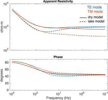
Figure 12 shows example FDEM responses at 2, 4 and 6 km offset centered over the lake. Despite the 2D lake geometry, these responses are qualitatively similar in magnitude and frequency behavior to the 1D responses shown in Figure 6. The largest anomaly between the dry and wet models occurs ~100 Hz with differences of up to 30% in amplitude and 6° phase at both 4 and 6 km offsets, while much smaller anomalies are seen at 2 km offset. The magnitude of these anomalies is smaller than that of the corresponding MT anomalies, suggesting that FDEM data are perhaps less ideal for subglacial mapping. However, we note that there may be practical advantages to collecting FDEM data: very large dipole moments could be generated using a strong source transmitter, so that the signal-to-noise ratio greatly exceeds that of MT data. In this case, the anomalies may in practice be relatively larger than the MT anomalies when measured relative to the data noise level.

Fig. 12. Amplitude and phase FDEM responses for data at 2, 4 and 6 km offset centered over the lake for our SLW-like domain (lake model) and in a similar model with the lake removed (dry model).

4.2. Grounding zone study

In this section, we conduct a model study to highlight how EM data can constrain hydrologic structure near the grounding line of an ice stream. We are motivated by recent observations of a subglacial estuary at the grounding zone of Whillans Ice Stream, where a combination of radio-echo sounding, kinematic GPS, and active-source seismic data were used to infer the existence of an estuary-like feature (Horgan and others, Reference Horgan2013); here, we show how EM data could be used to image such an estuary via the high conductivity of saline estuary water. Figure 13 shows the hypothetical model of grounding zone electrical resistivity. Our model, modified from an inversion of a ground-based gravity survey (Muto and others, Reference Muto, Christianson, Horgan, Anandakrishnan and Alley2013), consists of ~700 m of ice underlain by ~1 km of moderately porous sediments. Seaward of the grounding line, the model contains seawater-saturated marine sediments beneath a thin ocean cavity that is only a few meters thick. Landward of the grounding line, the shallow sediments are significantly more resistive, which could reflect either significantly fresher pore-water due to inflow from the upstream hydrologic system or from overall lower porosity. We include a seawater intrusion zone landward of the grounding line to represent an estuary with 1 m thickness and 5 km lateral extent. This feature could be transient, arising from a tidally driven pulse of seawater that moves inward from the grounding line (Horgan and others, Reference Horgan2013; Walker and others, Reference Walker2013). To demonstrate sensitivity to deeper components of the system, we added two relatively conductive 2 Ω-m prisms, labeled A and B, which represent high porosity (~20%) sandstones filled with conductive seawater. Since our previous model study shows similar results for both MT and FDEM data, here we only consider MT data. MT responses were generated at 36 frequencies spanning from 0.001 to 1000 Hz for 31 receivers spaced every 500 m along the ice surface.

Fig. 13. (a) Grounding zone model study. The model includes ~700 m of ice overlying 1 km of moderately porous sediments above a resistive basement. The grounding line is located at 0 km position. A conductive ~200 m thick layer of seawater-saturated marine sediments is underneath the floating portion of the ice. Two conductive prisms labeled A and B are located within the deeper sediments. White triangles show the MT receiver locations on the ice surface. (b) Close up of the ice base showing a 1–3 m thick ocean cavity to the right (downstream) of the grounding line and a 5 km wide by 1 m thick transient seawater intrusion zone to the left (upstream) of the grounding line.

Pseudosections of the MT response anomaly show the relative differences between the responses from models with and without the seawater intrusion are up to 25% (Fig. 14). Both TE- and TM-mode responses have anomalies that are primarily confined to receivers located over the seawater intrusion. The responses also exhibit TE- and TM-mode effects that are similar to those seen in our earlier subglacial lake study; for both TE and TM modes, there is a centrally located anomaly ~10–100 Hz, but at lower frequencies, the TM mode also has a frequency-independent anomaly consistent with a galvanic distortion of the EM field. The 25% peak anomaly magnitude from this 2D conductive structure is significantly smaller than the >100% anomaly predicted by the 1D sensitivity study in Figure 4, illustrating that the limited lateral extent of this feature reduces its overall impact on the MT response compared with a 1D layer. Even with a smaller magnitude anomaly, this experiment suggests that a continuously recording MT receiver deployed upstream of the grounding line could effectively identify transient seawater intrusions and help quantify potentially significant grounding zone processes.

Fig. 14. Relative anomaly in the MT responses due to the 1 m thick seawater intrusion at −5 to 0 km lateral position. The anomaly is calculated by taking the relative difference in the response from models with and without the seawater intrusion and is shown as a function of frequency and receiver position.

Figure 15 shows the result of inverting synthetic data that included 1% random Gaussian noise. The inversion was started from a uniform 100 Ω-m starting model, and the ice layer and ocean cavity were held as fixed structures with known resistivities. The inversion's smoothness constraint was relaxed along the base of the seawater intrusion zone, allowing for a sharp jump in resistivity, as was done previously in the subglacial lake study in Figure 9d. The broader view (Fig. 15a) shows that MT data can image all of the large-scale components of the original model: conductors A and B, the resistivity difference between the marine sediments and the sediments beneath the grounded ice, and the higher resistivity of the deeper low porosity basement. Details from the inversion near ice–bed interface (Fig. 15b) shows that the inversion recovered well the low resistivity in the seawater intrusion channel along its entire length.

Fig. 15. Electrical resistivity obtained by non-linear inversion of synthetic MT data generated for the grounding zone model. Panel (a) shows the deeper subglacial region, while (b) shows the detail recovered near the subglacial seawater intrusion zone at −5 to 0 km position. The inversion's smoothness constraint was relaxed along the base of the seawater intrusion zone to allow for a sharp jump in resistivity. The ice layer and ocean cavity were held as fixed structures with known resistivities. Black lines show the structural boundaries from the true model shown in Figure 13.

Despite the effective overall performance of this inversion for recovering model structure, it is worthwhile to consider some limitations of EM data. Comparison with the sharp boundaries of the original forward model shows a significant degree of lateral and vertical smoothing in the inverted resistivity that reflects the spatial resolution limits of diffusive EM data. The degree of smoothness in the inverted model can be used to infer limitations in the depth and lateral resolution of EM data. The grounding zone forward model contains sufficient space between the conductors, so they can be uniquely resolved in an inversion; however, if the conductors are too close together (vertically or laterally), the inversion would likely smooth them together into a single conjoined feature. Likewise, the forward model contains conductivity contrast between the conductors and the sediments that are at least an order of magnitude; smaller conductivity contrasts would be more difficult to image. However, despite the smoothed feature boundaries and resolution limitations, this experiment shows that MT data can be used to discern zones of high porosity from low porosity and between saline and fresh water components, and thus could be used for large-scale characterization of the hydrological regime at a grounding zone. Similar to the subglacial lake experiment, some of these limitations could be mitigated with additional knowledge of geologic structure from active-source seismic data.