2.1. Outlet glacier dynamics

In the current set-up, the 3-D ice-sheet model does not natively include a mechanism to account for the influence of oceanic forcing on marine-terminated outlet glaciers. Furthermore, the grid resolution of 5 km would be too coarse to simulate the processes at the marine ice front and at the grounding line with sufficient detail. Therefore, thinning and retreat rates of marine-terminated outlet glaciers in the large-scale ice-sheet model are prescribed, based on results from explicit simulations of four outlet glaciers with a state-of-the-art flowline model (Reference NickNick and others, 2013). Their flowline model takes into account the glacier’s SMB and submarine melt along a flowband and includes lateral, basal and along-flow stresses. Atmospheric and oceanic forcings are explicitly included and a dynamic calving law based on a stress criterion is used (Reference Nick, Vieli, Howat and JoughinNick and others, 2009). The simulated glaciers are Jakobshavn Isbræ (JKB), Petermann Glacier (PTMN), Kangerdlugssuaq Glacier (KNG) and Helheim Glacier (HH), for all of which full drainage basins are included in the model domain. The flowline model is forced with different types of atmospheric and oceanic data from global and regional climate and ocean models (Reference NickNick and others, 2013). The SMB and atmospheric forcings for the future period are derived from the regional climate model MAR (Modèle Atmosphérique Régional) under the A1B forcing scenario, the same as described below for the large-scale model. The flowline model has been tuned individually for each glacier to best reproduce observations of velocity change and retreat/advance rates for the period 2000–10 by modifying the relative importance of different climatic processes (Reference NickNick and others, 2013). Uncertainty in the weight of the different processes and in model parameters is expressed by five available future retreat scenarios for each glacier. Until ad 2100 there is relatively little change projected for the four glaciers compared to larger retreat rates in the 22nd century.

For the current work the scenarios that produce medium sea-level changes by ad 2200 for each glacier are selected. The two extreme scenarios, which yield the largest and smallest mass loss by 2200 under parameter variations but still reproduce the observed behaviour, are additionally evaluated to quantify a range of possible responses. We use (1) modelled grounding line positions and (2) thinning rates at the grounding line from these flowline model results to force the large-scale ice-sheet model. To incorporate the results of the modelled glaciers, the moving grounding line position of the flowline model is interpolated to the coarser grid of the ice-sheet model and grounding line thinning rates are applied there. Incidentally, these thinning rates include a SMB component, which is, however, small compared to the dynamic component. Thinning rates further inland result from dynamic adjustment, within the 3-D large-scale model, to this marginal forcing and are not prescribed. Ice is always removed downstream of the grounding line and when reaching flotation. To calculate the sea-level contribution, an additional correction is made for the ice column at buoyancy that is merely replaced by sea water.

In order to extend the forcing to other, marine-terminated outlet glaciers, thinning and retreat rates are generalized per region to all gridpoints that are grounded below sea level and are in contact with the ocean. To avoid influence of smoothing of topographic features during interpolation, we initially perform the selection of forcing points on the original 1 km dataset. We then select the number of forcing points on the interpolated 5 km grid to cover the same area as the selected points on 1 km resolution. For that purpose, we calculate the ratio of selected versus total 1 km gridpoints per 5 km gridbox ‘R’ and globally adjust a threshold ratio R _threshold necessary to classify it as forcing point. The derived R _threshold = 0.8 = 20/25 has proven to be robust to changes in how far inland forcing points are selected by the search routine. Given the coarser resolution of the large-scale model and the absence of reliable bathymetry data for most of these areas, along-flow retreat lines are defined off line for all selected gridpoints. For all glaciers in the same region, thinning rates are prescribed for the last grounded gridpoint along their respective retreat lines equal to the explicitly modelled glacier of that region. Ice is again removed downstream from the grounding line and when reaching flotation. In order to additionally force all marine-terminated outlet glaciers represented on the 1 km grid but that fall below the 5 km grid resolution, we apply partial thinning (and retreat) for all 5 km gridpoints below the threshold value according to the ratio R. ‘Partial retreat’ is implemented as a one-time additional thinning of magnitude H·R, where H is the local ice thickness.

PTMN rates are used to force the northern and northeastern glaciers, JKB rates for the western glaciers, HH rates for the southeast, and KNG rates for the central east, following the regional categories of Reference Rignot and MouginotRignot and Mouginot (2012). The applied regional grouping is motivated by a similar geophysical setting (accumulation regime, surface slope) of the explicitly modelled and generalized glaciers for each region. The northern glaciers are predominantly iceshelf-terminated with relatively low velocities compared to most other Greenland marine-terminated glaciers. Calving glaciers in the central east have predominantly lower velocities compared to glaciers in the southeast and northwest, which is mainly determined by the different amounts of accumulation in these sectors (Reference Moon, Joughin, Smith and HowatMoon and others, 2012). Figure 1 displays all gridpoints that are fully or partially forced in the model to document the selection procedure.

Fig. 1.

Overview of outlet glacier forcing locations on the large-scale model grid. Lines show the centre lines of the four explicitly modelled glaciers from the flowline model (Reference NickNick and others, 2013). Shaded regions indicate the gridcells that are removed due to outlet glacier retreat and thinned over the course of the experiment. Locations of gridcells with partial thinning and retreat and respective forcing ratios are indicated by filled circles. Colour indicates grouping of forcing regions discussed in the text.

Prescribing and generalizing thinning and retreat rates at the ice-sheet margin in the above way primarily aims to estimate large-scale 3-D effects and possible feedbacks on the inland ice flow (marginal adjustment and inland propagation of thinning waves), rather than the details of individual glaciers.

2.2. Meltwater lubrication of the base

The effect of basal lubrication on ice velocity is taken into account with a parameterization (Shannon and others, in press). It is assumed that all runoff can penetrate locally to the bed and changes the sliding velocity according to observed relations between runoff and speed-up. Shannon and others (in press) tested a large range of runoff–speed-up relations with four different ice-sheet models, including the model from the present work. Their results indicate that the additional contribution of basal sliding to future sea-level rise is very limited for the whole range of plausible runoff–speed-up relations and the studied range of ice-sheet models. Therefore, only the runoff–speed-up relation that best matches observations is used here and the reader is referred to Shannon and others (in press) for a detailed uncertainty analysis. The relation predicts limited speed-up at high values of runoff, in line with some observations (Reference Van de WalVan de Wal and others, 2008; Reference Sundal, Shepherd, Nienow, Hanna, Palmer and HuybrechtsSundal and others, 2011) and theoretical arguments (Reference SchoofSchoof, 2010). In our model, meltwater lubrication is implemented by extending a common Weertman sliding relation (e.g. eqn (A8) of Reference Huybrechts and de WoldeHuybrechts and de Wolde, 1999) with a multiplier S _BL that changes with runoff from 1.0 at ad 2000 to a maximum of 1.3 for some locations:

where , , H and h are sliding velocity, non-local higher-order basal drag, ice thickness and bed elevation, respectively, and A _s = 0.83 × 10⁻¹⁰ m⁸ N⁻³ a⁻¹, ρ = 910 kg m⁻³ and g are the sliding factor, ice density and gravitational acceleration, respectively. Division of A _s by H serves to generate increased sliding velocities towards the ice-sheet margin.

3.1. Regional climate model

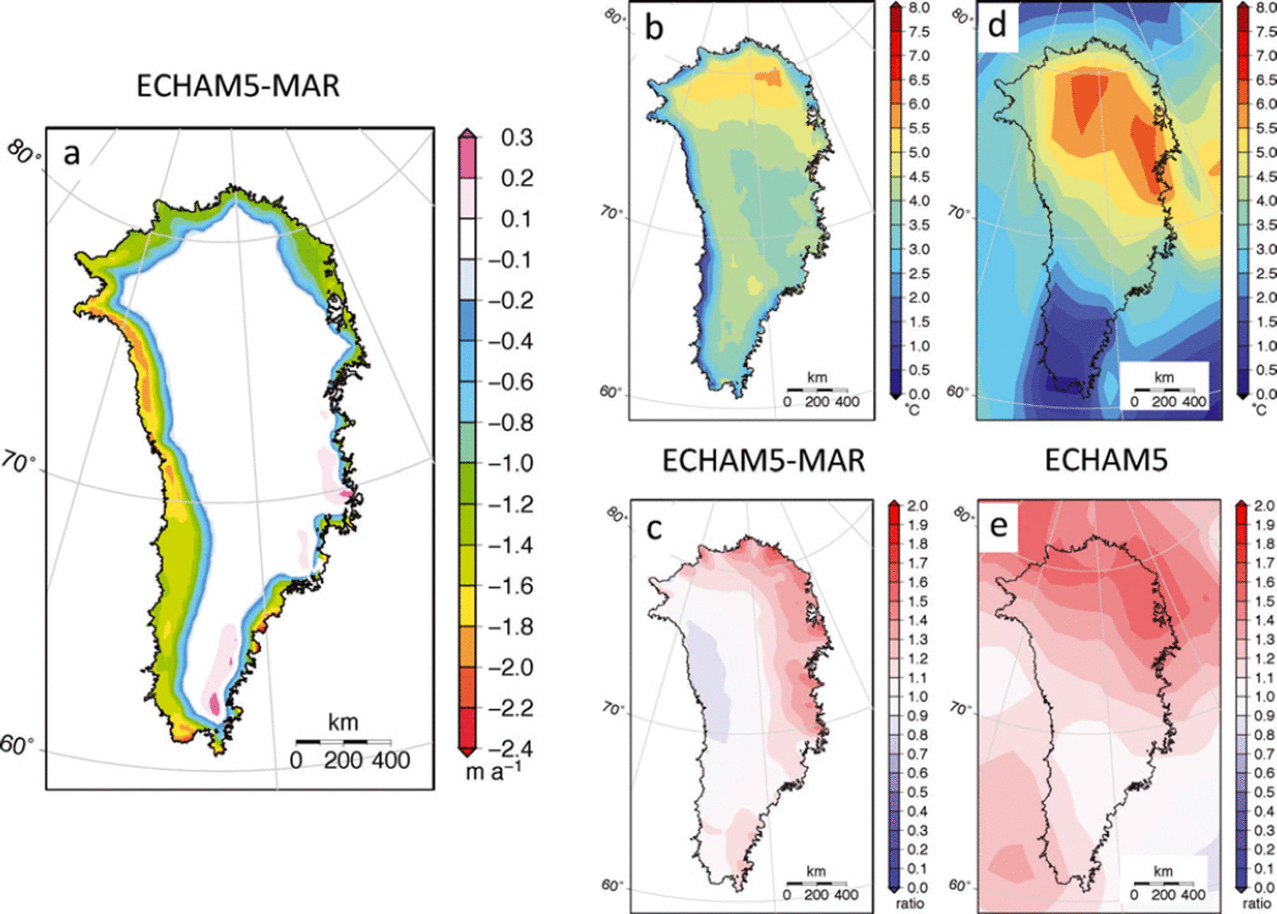
The SMB forcing of the reference model is derived from annual SMB simulated at 25 km resolution by the regional climate model (RCM) MAR (Reference FettweisFettweis, 2007), which is forced at the lateral boundaries by 6 hourly output from the global general circulation model (GCM) ECHAM5 for SRES scenario A1B. The MAR model has been chosen because it performs well in recent-past simulations (Reference RaeRae and others, 2012). It is fully coupled with a complex snow model taking into account the positive albedo feedback and has been intensively validated over the GrIS (Reference Fettweis, Tedesco, Van den Broeke and EttemaFettweis and others, 2011). Since ECHAM5 underestimates the atmospheric dynamics (i.e. wind speed) and its atmosphere is too warm in summer over the GrIS with respect to the European Centre for Medium-Range Weather Forecasts (ECMWF) ERA-40 reanalysis over 1980–99, MAR forced by ECHAM5 overestimates the melt in summer and is too dry with respect to the ERA-40 forced MAR simulation (Reference RaeRae and others, 2012; Reference FettweisFettweis and others, 2013). For this reason, SMB anomalies are used instead of absolute SMB values as forcing for future projections. Anomalies are calculated against a mean 1989–2008 reference SMB. For comparison, the SMB decrease projected by MAR with ECHAM5 boundary conditions for scenario A1B (Fig. 2a) is in the lower range of the CMIP5 forced MAR simulations for the RCP8.5 scenario (Reference FettweisFettweis and others, 2013). Runoff forcing for the basal lubrication parameterization in all experiments is derived from the same MAR model run.

Fig. 2.

Yearly SMB anomalies (a), summer (June–August) temperature anomalies (b, d) and yearly precipitation ratios (c, e) for SRES scenario A1B from ECHAM5-MAR (a–c) and ECHAM5 (d, e) calculated for the 2091–2100 average with respect to the 1989–2008 average of the reference state.

In order to overcome a small mismatch of the ice-sheet mask between RCM and ice-sheet model, the SMB data have been extended by assuming a linear SMB gradient with height from surrounding ice-covered points. RCM-SMB data have been bilinearly interpolated to the 5 km ice-sheet model grid.

3.2. Positive degree-day model

The second SMB model used in this study for comparison is a classical positive degree-day (PDD) model that calculates surface melt and runoff from the integrated sum of expected positive degree-days. These are a function of a sinusoidal seasonal cycle and an assumed variability of daily near-surface temperatures about the monthly mean temperature. The model considers different degree-day factors (DDFs) for snow and ice to implicitly deal with their different albedos. The applied DDFs (2.7 and 7.2 mm w.e.d⁻¹ °C⁻¹ for snow and ice melting, respectively) and the standard deviation to account for the daily cycle and weather variations (σ = 4.2°C) are identical to those used in previous studies with the same model (Janssens and Huybrechts, Reference Janssens and Huybrechts2000; Gregory and Huybrechts, Reference Gregory and Huybrechts2006; Hanna and others, Reference Hanna2011).

The runoff model incorporates a simple one-dimensional snowpack model. In the snow-covered region, meltwater from surface melting is initially stored as capillary water within the snowpack. Eventually, the snowpack becomes saturated and runoff occurs, although melt needs to reach typically 60% of the annual precipitation before this can happen (Janssens and Huybrechts, Reference Janssens and Huybrechts2000). Rain contributes to any retention or runs off. The runoff/retention scheme also accounts for superimposed ice formation and subsequent melt. The model is forced with monthly temperature anomalies and yearly precipitation ratios calculated against the same reference period as for RCM-SMB (ad 1989–2008). Temperature and precipitation data for the future period are derived either from the ECHAM5-forced RCM MAR or directly from the GCM ECHAM5 itself. The PDD model is also used for spin-up of the ice temperature and for initialization over the ERA-40 period. The height–SMB feedback is automatically included through the dependence of surface temperature on ice-sheet elevation by means of the atmospheric lapse rate.

4.1. Model initialization

The classical approach to initialize ice-sheet models for future sea-level projections stems from palaeo-applications and consists of a spin-up over one or several glacial–interglacial cycles (Huybrechts, Reference Huybrechts2002). The advantage of such techniques is that the ice sheet is always in a self-consistent state concerning SMB, ice temperature, ice thickness and velocity, and furthermore carries its long-term memory with it. The shortcoming of such a freely evolving model, however, is that the observed surface elevation and consequently the ice sheet’s flow characteristics do not exactly match the observations. Often, the modelled present-day ice sheet is somewhat too large and exhibits margins that are too thick (Reference HuybrechtsHuybrechts, 2002; Reference Greve, Saito and Abe-OuchiGreve and others, 2011; Reference Robinson, Calov and GanopolskiRobinson and others, 2011), even if this mismatch can be partially reduced by distributed tuning of outlet glacier velocities (Reference Graversen, Drijfhout, Hazeleger, Van de Wal, Bintanja and HelsenGraversen and others, 2011). This mismatch may introduce biases for future projections in terms of ice dynamics, since ice thickness and surface slope determine the driving stress, and hence the ice flow. SMB trends can be equally affected as they scale to the total melting volume and the size of the ablation area.

These shortcomings generated attempts to initialize large-scale ice-sheet models to match much more closely the observed geometry and velocity (Reference Arthern and GudmundssonArthern and Gudmundsson, 2010; Reference Price, Payne, Howat and SmithPrice and others, 2011; Reference Larour, Seroussi, Morlighem and RignotLarour and others, 2012). A fixed initial ice-sheet area also makes it possible to take advantage of forcing data from high-resolution RCMs run on the same observed ice-sheet mask. The inherent problem in this approach is that the flow field is initially not in equilibrium with the observed geometry. This also affects the ice temperature because of the advection terms that cannot be well defined. When imposing the continuity equation, a model drift is created to restore the equilibrium between local SMB and the divergence of the ice mass flux. This drift includes a real local ice thickness imbalance, but most of it is artificial and due to incomplete physics or uncertainties in the geometric data. A common way to deal with this issue is to defer most of the mismatch to the less constrained model parameters that control basal drag (Reference Price, Payne, Howat and SmithPrice and others, 2011; Reference Larour, Seroussi, Morlighem and RignotLarour and others, 2012; Reference Seddik, Greve, Zwinger, Gillet-Chaulet and GagliardiniSeddik and others, 2012) and/or ice temperature (Reference Arthern and GudmundssonArthern and Gudmundsson, 2010). In most cases, some relaxation of the model is still necessary to let it adjust to the imposed SMB. Remaining model drift can then be efficiently reduced by imposing a correction term to the SMB of similar magnitude to the imbalance inferred from observations (Reference Price, Payne, Howat and SmithPrice and others, 2011).

The limitation of applying constraints or corrections during initialization is that they have to be maintained for the whole duration of a prognostic experiment. This inherently assumes that the parameters or correction fields fixed for the present day do not vary over the time period of the simulation. Given the dominant adjustment timescales of ice sheets of the order of 1000 years, the validity of such initialization methods is limited to projections on centennial timescales.

Our initialization of the ice-sheet model here combines elements of the procedures described above, but proceeds without additional tuning to observed velocities of individual outlet glaciers. This avoids biases from observational uncertainties and of recent marginal variability in outlet glacier speeds. First the ice temperature is derived from a palaeo-spin-up over several glacial–interglacial cycles to account for past, long-term climate changes. The temperature field is subsequently rescaled to the observed ice thickness. Basal ice temperatures from the spin-up are corrected for the pressure-melting point associated with the different ice thickness, and surface temperatures are adapted to the observed surface elevation. Vertical temperature profiles are then slightly adjusted to adapt to the new boundary conditions, but the shape of the profile is kept. Any mismatch between the mask for the spin-up experiment and the observed surface area is resolved by searching nearby locations with similar surface elevation as proxy for missing temperature data. The ice temperature serves to determine the ice hardness and the area of basal sliding, and is kept constant over the course of the experiments. Since ice temperature is a slowly changing quantity, this has a negligible effect on the large-scale ice-sheet response.

Secondly, an often-made assumption is made that the GrIS was in steady state with SMB for the period 1960–90 (e.g. Reference Hanna, Huybrechts, Janssens, Cappelen, Steffen and StephensHanna and others, 2005). A reference SMB for this period is derived with the PDD model forced by ECMWF ERA-40 reanalysis data (similar to Reference HannaHanna and others, 2011) for the observed surface elevation. The ice-sheet geometry is relaxed with this imposed SMB field as a boundary condition during a time-dependent model run for 1000 years. For this run ice temperature, bedrock elevation and ice-sheet mask are fixed and ice-thickness changes are limited to 0.2 m a⁻¹. Consequently, any deviation from the observed geometry at the end of the run is nowhere more than 200 m and in 80% of the ice sheet less than ±50 m. When the ice sheet relaxes towards the unconstrained model geometry, it turns out that the 5% of the ice-sheet area with positive deviations of >150 m is exclusively located at the margin, as expected. Such ice thickness corrections are similar in the higher-order approach to the force balance compared to a shallow-ice model. Horizontal stress gradients were expected to remove some of the inherent model imbalance initially present, but this is not effective on a 5 km grid.

Thirdly, a synthetic SMB correction is determined to effectively remove any remaining model drift and impose a steady state for the reference SMB forcing (1960–90). We extend the method used by Reference Price, Payne, Howat and SmithPrice and others (2011) with an iterative procedure. A first-guess SMB correction is diagnosed as the remaining ice thickness imbalance after the first year of an unforced experiment, in which the area constraint has been lifted. The same experiment is then repeated five times, in which the previous SMB correction is applied each time and then updated by adding the remaining imbalance after 10 years. The final SMB correction is on average 9 cm a⁻¹, with <0.3% of the total ice-sheet area having a correction of >10 m a⁻¹, predominantly at marine-terminated ice margins. For these locations the synthetic SMB correction can be considered as an additional ice thinning or thickening from dynamic discharge that is not intrinsically simulated due to approximations made at the ice-sheet boundary (e.g. Reference Saito, Abe-Ouchi and BlatterSaito and others, 2007). An unforced control experiment with the resulting SMB correction exhibits a negligible mass drift of ∼0.2 mm sea-level equivalent (s.l.e.) over 200 years.

The model including the SMB correction is then finally run from ad 1958 to 2010 with a combination of ECMWF ERA-40 and ERA-Interim reanalysis data (Reference HannaHanna and others, 2011). Assuming a steady state for the 1960–90 reference period, this gives rise to an imbalance due to past SMB changes for the ice-sheet projections starting in the year 2000. This neglects an additional ice-dynamic background trend from the long-term evolution of the GrIS as far back as the last glacial period, but such a trend has been found to be very small (<0.05 mm s.l.e. a⁻¹; Reference Huybrechts, Gregory, Janssens and WildHuybrechts and others, 2004).

4.2. Future climate forcing

For future projections of the ice-sheet evolution starting at ad 2000, the yearly SMB forcing (Fig. 2a) is derived from the ECHAM5-forced MAR under SRES scenario A1B (RCMSMB). For comparison, we additionally use the PDD model to calculate the SMB with monthly temperature anomalies and yearly precipitation ratios (Fig. 2b–e) from either MAR (RCM-PDD) or directly from the underlying GCM ECHAM5 (GCM-PDD). Since ECHAM5 data were only available until ad 2099, the RCM and GCM forcing is extended in all three SMB versions from ad 2100 onwards by repeating the years 2090–99 until ad 2200.

The reference model is forced with RCM-SMB anomalies calculated against the average SMB over the ad 1989–2008 reference period (ΔSMB(1989–2008)_RCM). A correction is added to account for the SMB difference between the two reference periods (ad 1960–90 and 1989–2008) as calculated with the PDD model (ERA-PDD). This re-referencing step is necessary because the ice sheet is initialized to be in steady state with the ERA-PDD SMB 1960–90. The SMB anomaly for the future period is therefore

where and are SMB averages over the specified time periods of ERA-PDD. Since SMB anomalies are added to the used during initialization, the total SMB for the future simulations simplifies to

For the PDD approach, the SMB (SMB_PDD) is calculated relative to the ad 1989–2008 average of temperature and precipitation. The same re-referencing correction as above is applied to the resulting SMB forcing:

where ΔSMB(1989–2008)_PDD is the SMB anomaly of the PDD model calculated against a reference SMB_PDD for a fixed initial (ad 2000) surface elevation.

In summary this means that all SMB schemes (RCM-SMB, RCM-PDD, GCM-PDD) show identical behaviour in unforced control experiments. Results of the different schemes depend on anomalies (ratios) in SMB and temperature (precipitation) and can be compared quantitatively.

5.1. Present-day evolution (1958–2010)

Figure 4 shows present-day volume change (mm s.l.e.) for three treatments of the forcing. Up to ad 2000, ice-sheet volume changes are uniquely determined by the imposed SMB changes from the PDD model, assuming no mass change for 1960–90. After 2000, the forcing switches to RCM SMB anomalies in the reference model, which has an additional forcing from the prescribed outlet glacier evolution. Also shown are the results from an alternative SMB forcing series from RCM-PDD.

Fig. 4.

Recent GrIS contributions to global sea-level change forced with ERA data between 1958 and 2010 with a positive-degreeday model (ERA-PDD), with SMB anomalies from a regional climate model including ice dynamics and outlet glaciers (Reference model), and with SMB forcing derived from a positive-degree-day model forced with climate anomalies from a regional climate model (RCM-PDD).

Sea-level contributions for the ERA period (1958–2010) calculated with the PDD model are similar to those implied by Reference HannaHanna and others (2011) by construction, as the runoff model and the ERA forcing data are the same. However, in our study we use an anomaly scheme and a surface temperature parameterization as in Reference Wake, Huybrechts, Box, Hanna, Janssens and MilneWake and others (2009), whereas Reference HannaHanna and others (2011) downscale surface temperature and net precipitation directly from the reanalysis data. For the decade 2000–10, all three experiments shown in Figure 4 have a rapid increase in sea-level contribution. This is due to an increase in meltwater runoff and, to a lesser extent, to a decrease in precipitation compared to the 1990s, similar to the relative importance of the two processes shown in Reference Van den BroekeVan den Broeke and others (2009). A larger trend for the two projections involving the RCM (RCM-SMB for the reference model and RCM-PDD) compared to ERA arises mainly from outlet glacier thinning and, to a lesser extent, from the SMB difference between the 1960–90 and 1989–2008 reference periods.

The total simulated sea-level trend of ∼0.2 mm a⁻¹ is biased low compared to estimates of the decadal (2000–10) mass loss of 0.45 ± 0.2 mm a⁻¹ (Reference Rignot, Velicogna, Van den Broeke, Monaghan and LenaertsRignot and others, 2011; Reference ZwallyZwally and others, 2011; Reference ShepherdShepherd and others, 2012), but increases to 0.42 mm a⁻¹ for the decade ad 2010–20. By then the trend arises in approximately equal share from outlet glacier acceleration and SMB changes in line with reconstructions for the recent past (Reference Van den BroekeVan den Broeke and others, 2009). Results for the four explicitly modelled outlet glaciers from the flowline model indicate a mass loss of 0.056 mm a⁻¹ over the period 2000–10 (Reference NickNick and others, 2013). When the associated outlet glacier retreat is interpolated to the coarser resolution of the large-scale model, a delay of the response is introduced until retreat has occurred over an entire 5 km gridcell. This initial bias is, however, of absolute nature and is rendered insignificant by the large retreat rates over the remainder of the experiment.

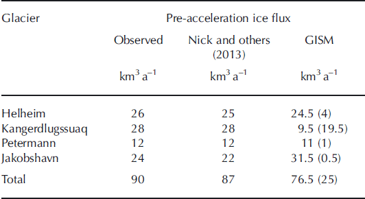
Simulated present-day fluxes for the major outlet glaciers in the large-scale model are in good agreement with observations (Table 1) and Reference NickNick and others (2013), except for Kangerdlugssuaq (KNG). The flux of the latter shows only one-third of the observed magnitude. Due to mass conservation, the remaining mass loss for this glacier occurs through the synthetic SMB correction over the terminal part of the drainage basin and is therefore constant over time. To a much smaller extent this is also the case for Helheim Glacier and negligibly so for Jakobshavn Isbræ and Petermann Glacier. A low flux bias from KNG is also found in another, higher-resolution full-Stokes model using the same geometrical input data (Reference Gillet-ChauletGillet-Chaulet and others, 2012), which may point towards a common prohibiting feature.

Table 1.

Pre-acceleration ice fluxes from the four explicitly modelled outlet glaciers from observations, flowline model and large-scale model GISM. For the latter, additional flux exported by the synthetic SMB correction is given in parentheses

Given the grid resolution of 5 km and the fact that no additional tuning was applied, the initialized ice velocity for the start of the prognostic experiments in ad 2000 (Fig. 5) is in reasonably good agreement with inferences made from satellite radar interferometry (Reference Joughin, Smith, Howat, Scambos and MoonJoughin and others, 2010; Reference Moon, Joughin, Smith and HowatMoon and others, 2012). The model, however, does not represent the ‘North East Greenland Ice Stream’ (NEGIS) well. The presence of this feature in balance velocity calculations using the observed surface topography (Reference Joughin, Fahnestock, Ekholm and KwokJoughin and others, 1997) suggests that it must have been lost during the relaxation phase of the initialization due to a smoothing effect on surface elevation. The hypothesis that enhanced basal lubrication from melting across a basal hot spot is responsible for the high velocities (Reference Fahnestock, Abdalati, Joughin, Brozena and GogineniFahnestock and others, 2001) may explain why our model cannot represent NEGIS without additional tuning.

Fig. 5.

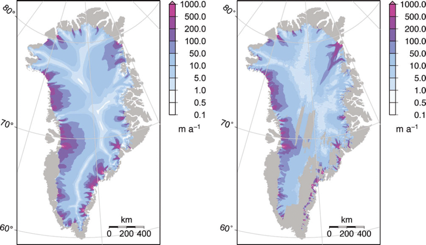
(a) Surface velocity magnitude arising from the initialization procedure in the reference model at ad 2000, and (b) observed interferometric synthetic aperture radar (InSAR) velocities (Reference Joughin, Smith, Howat, Scambos and MoonJoughin and others, 2010).

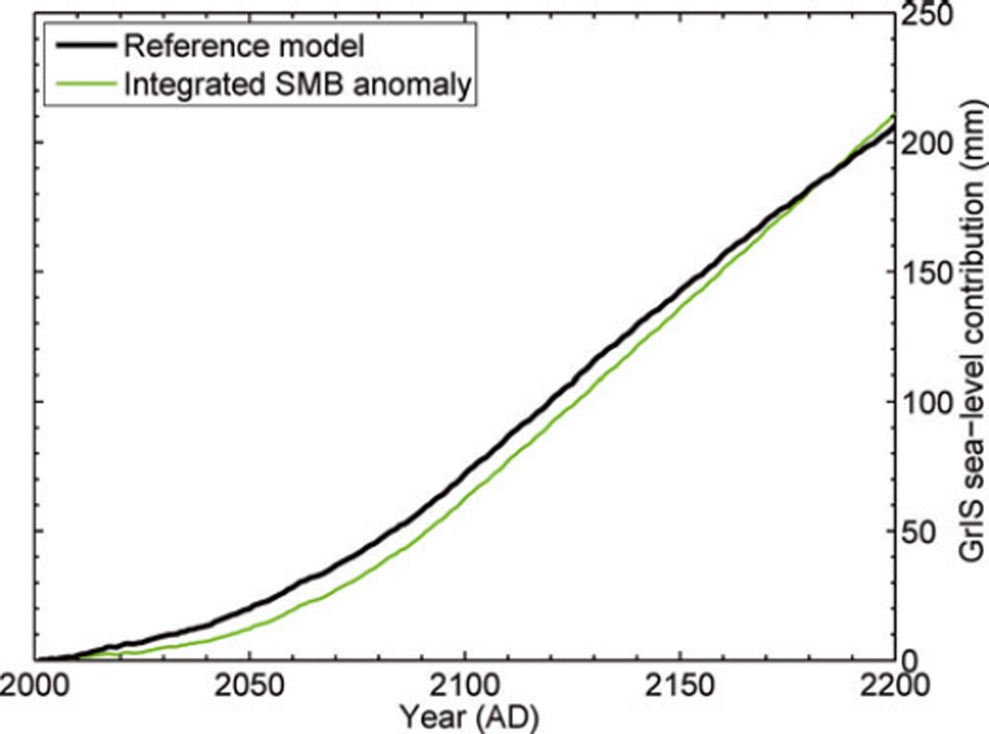
5.2. Reference projection

The combined effect of SMB (including SMB–height feedback), outlet glacier retreat and basal lubrication results by ad 2100 in a sea-level contribution of 7.2 cm (Fig. 6). The rate increases during the 21st century but becomes approximately constant during the 22nd century when the forcing stabilizes at the 2090–2100 level, except for episodic outlet glacier retreat followed by geometric adjustment as the thinning is propagated inland. By ad 2200 the sea-level contribution is 20.7 cm, similar to the time-integrated SMB anomaly (21.1 cm). The resulting pattern of ice thickness change (not shown) is governed by overall marginal thinning, complemented by thickening in some regions of the accumulation zone where positive SMB anomalies are present (Fig. 2a).

Fig. 6

Sea-level contributions projected with the reference model including ice dynamics and prescribed outlet glacier retreat compared to the time-integrated SMB anomaly as a measure of the direct SMB effect.

6.1. Surface mass balance

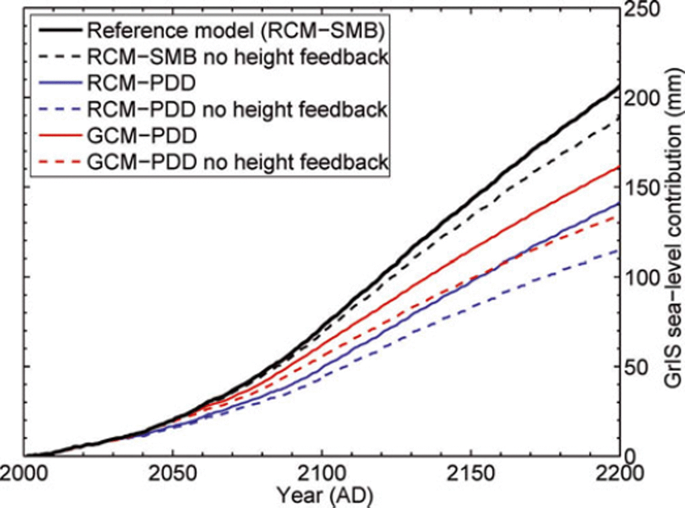
Figure 7 shows the results from different methods of dealing with the SMB forcing. All the options we investigated result in a lower response than the reference run. Modelling the SMB with a positive-degree-day method driven by temperature and precipitation anomalies from the same regional climate model (RCM-PDD) results in a 2.3 cm (6.5 cm) lower sea-level contribution in ad 2100 (ad 2200), or ∼30% less than the reference model (RCM-SMB). This is directly caused by a weaker decrease of the SMB and over a smaller area in RCM-PDD as compared to RCM-SMB. A closer inspection of the spatial patterns of the two SMB anomaly fields (Figs 8a and 2a) suggests a strong influence of the SMB diagnosed for the two models for their own ad ∼2000 reference state. The SMB models differ in their location of the equilibrium line (where SMB = 0) across the ice sheet, and this translates directly to their respective anomaly patterns. This is, for example, the case for large regions in the north, where a moderate temperature increase in ECHAM5-MAR (Fig. 2b) has a limited impact on RCM-PDD as summer temperatures remain below the freezing point. A different treatment of refreezing, which has been shown to account for large differences between some SMB models (Reference BougamontBougamont and others, 2007), is not important for the comparison between RCM-SMB and RCM-PDD. Only a narrow marginal region in the south and southeast shows significantly different refreezing changes between the two models, where up to 40% of the lower SMB anomalies in RCM-PDD are explained by a decrease in refreezing.

Fig. 7

Comparison between different methods of applying the SMB forcing from the same climate models for SRES scenario A1B. The dashed lines do not consider the feedback between surface elevation and mass balance. Table 2 has more details of the different model set-ups.

Table 2.

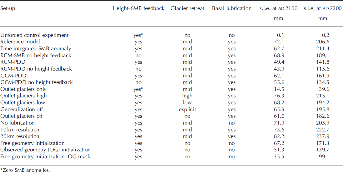
Overview of the various set-ups to investigate the GrIS contribution to global sea-level rise by the years ad 2100 and ad 2200. All s.l.e. figures consider only ice loss above flotation after calving fronts retreat

Fig. 8

Average SMB anomalies obtained with the PDD model using climate anomalies from (a) ECHAM5-MAR and (b) ECHAM5. These are for the decade 2091–2100 relative to the 1989–2008 reference period. SMB is calculated for a fixed surface topography (excluding height–mass-balance feedback) to allow comparison with Figure 2a.

Perhaps the most striking difference between RCM-SMB and RCM-PDD patterns is the lower amplitude of negative anomalies in RCM-PDD for most of the western side of the ice sheet. This is linked to the low surface temperature anomalies (<1–2°C) in ECHAM5-MAR (Fig. 2b). The surface temperature of melting snow/ice is limited to the freezing point (the energy in excess is used for melting snow/ice), and the surface temperature is already near 0°C over current summers. This dampens the near-surface temperature increase from which the PDD model then calculates the melt, compared to further melt increase calculated from the energy-balance-based model (Reference FettweisFettweis and others, 2013). Additionally, it is in this area that MAR projects the highest surface albedo decrease due to bare-ice expansion in summer (Reference Franco, Fettweis and ErpicumFranco and others, 2013), which accelerates the surface melt increase with respect to a temperature-dependent PDD model. This feedback explains why MAR projects an acceleration of surface melt increase with rising near-surface temperatures (Reference FettweisFettweis and others, 2013; Reference Franco, Fettweis and ErpicumFranco and others, 2013). Differences between the two SMB models are probably also influenced by model resolution, bearing on the detail in which the marginal ablation zones can be resolved (typically 20–80 km wide). MAR is implemented on a 25 km resolution, whereas the PDD model captures height differences on the 5 km grid of the ice-sheet model, most important for the lapse rate. This limitation of RCM-SMB could partially be overcome by applying a dynamic SMB parameterization (Reference EdwardsEdwards and others, 2013a) to re-estimate the SMB on a higher-resolution topography.

Using temperature and precipitation data directly from ECHAM5 to force the PDD model (GCM-PDD), on the other hand, results in a 13 mm (20 mm) larger sea-level contribution compared to RCM-PDD by ad 2100 (ad 2200). Here the SMB differences (Fig. 8) can be directly related to the different climate anomaly patterns produced by either ECHAM5 or ECHAM5-MAR (cf. Fig. 2). The ice-sheet topography is quite poorly resolved in ECHAM5, and this results in a qualitatively different temperature pattern, especially during the summer months when it matters most for runoff. Interior temperature anomaly magnitudes also differ by 2–4°C, but these have almost no effect on SMB as summer temperature remains well below the freezing point. It can be expected that the quality of runoff estimates in GCM-PDD methods would generally deteriorate with lower resolution of the GCM, as climate anomaly patterns tend to get ‘smeared out’, especially around the ice-sheet margin. For that reason, atmosphere–ocean GCM-based temperature index methods have usually tried to incorporate higher-resolution time slices at T106 spectral resolution (∼100 km horizontal grid size) or better (Reference Huybrechts, Gregory, Janssens and WildHuybrechts and others, 2004; Reference Gregory and HuybrechtsGregory and Huybrechts, 2006).

Precipitation changes appear to have a much smaller impact on RCM-PDD and GCM-PDD SMB anomalies. In spite of generally positive precipitation ratios almost everywhere in ECHAM5 (Fig. 1e), this has little impact on SMB and sea-level rise as the highest ratios occur in the northern part that also has the lowest accumulation rate. ECHAM5-MAR even simulates decreasing precipitation over the western margin, but its effect on SMB is more than outweighed by the smaller associated summer warming compared to ECHAM5.

It is not straightforward to draw a general conclusion of this SMB sensitivity study on previous work done for the IPCC, which was based on a hybrid application of GCMPDD (higher resolution for time slice patterns, lower resolution for the time series) but used identical parameters for the PDD model (Reference Gregory and HuybrechtsGregory and Huybrechts, 2006). Also, our results rely on only one combination of RCM and GCM, and the SMB behaviour may not be robust for other models. But if our results are any guide, the underestimate of the GrIS contribution to sea-level change by 2100 implied by IPCC methods may be anywhere between GCM-PDD (14%) and RCM-PDD (31%). Matching the sea-level response by 2100 of GCM-PDD and RCM-PDD to RCM-SMB would require an increase of the DDFs by 7% and 19%, respectively. This conclusion contradicts the findings of Reference BougamontBougamont and others (2007), who made a comparison between a degree-day model and an energy-balance model of Greenland’s SMB and found the PDD model to be twice as sensitive to future climate changes as the more comprehensive mass-balance model. However, the energy-balance model in Reference BougamontBougamont and others (2007) was forced by monthly anomalies from a GCM, and surface–atmosphere interactions such as the albedo feedback were not taken into account.

When the height–mass-balance feedback is not included in any of the SMB models, projected sea-level rises are 8–18% lower after 200 years, as expected (Fig. 7). The difference increases with time and is smaller for the dynamic SMB parameterization employed for RCM-SMB than for the PDD-based SMB models, which are directly sensitive to a temperature increase. The effect is almost entirely confined to the ablation zone, as elevation changes and absolute SMB in the ice-sheet interior (accumulation zone) are an order of magnitude lower than in the ablation zone. Additional elevation changes, from ice-dynamic adjustment of the flow field to the anomalous height changes caused by these SMB changes, were, however, found to be of minor importance (not shown). The role of the height–mass-balance feedback in total sea-level rise is very similar for RCM-PDD and GCM-PDD (5–6 mm s.l.e. by ad 2100, and 26–27 mm by ad 2200). In view of their different SMB anomaly patterns, this similarity seems to be coincidental, indicative of mutually opposing effects when averaged over the entire ice sheet.

Despite a limited effect of the height–mass-balance feedback on sea-level projections until ad 2100 (∼10% of total response), it is important to take it into account, especially on timescales beyond the 21st century as elevation changes then become more pronounced.

6.2. Outlet glacier dynamics

From Figure 9, it can be inferred that the additional sea-level contribution from outlet glacier dynamics is 11 mm at ad 2100 and increases to 24 mm by ad 2200 in the reference model. The large increase of additional mass loss in the 22nd century is a direct consequence of the prescribed outlet glacier evolution of the flowline model (Reference NickNick and others, 2013). The mass loss is not continuous and is punctuated by episodic and rapid retreat of the outlet glaciers, visible as step increases in sea-level rise in Figure 9. They are mainly a consequence of quantization when interpolating the retreat from the flowline model to the coarser ice-sheet model grid, but would also arise at a higher resolution from calving fronts retreating rapidly across overdeepened fjord sections, albeit with smaller amplitude (Reference Nick, Vieli, Howat and JoughinNick and others, 2009). In the experiments, the effect of prescribing the retreat of the outlet glaciers is far more important for the large-scale ice mass loss than the effect of the prescribed thinning.

Fig. 9.

Effect of outlet glacier dynamics on the large-scale response of the GrIS. Uncertainty in the glacier retreat scenarios is represented by complementing the reference model by two extreme cases with high (dot-dashed black) and low (dashed black) retreat rates. For comparison the cases are also shown without SMB changes (green), with prescribed outlet glacier generalization switched off (red), and with prescribed outlet glacier dynamics switched off altogether (blue). The difference between the reference model and the model run without prescribed outlet glacier dynamics is also given (orange).

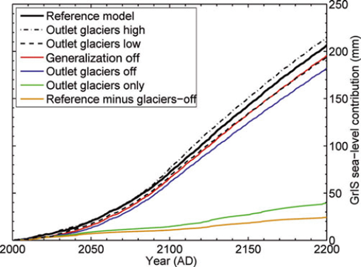
The sensitivity of the large-scale ice-sheet projections to uncertainty in outlet glacier treatment can be quantified by comparing the medium retreat scenario of the reference model against alternative minimum and maximum retreat scenarios (Fig. 9). The resulting range of outlet glacier contributions to sea-level rise is 7–15 mm at ad 2100 and increases to 12–32 mm by ad 2200. The additional uncertainty introduced by extending the response of only four glaciers to the entire ice sheet can, however, not be captured rigorously, but is believed to be to some extent covered by the range of physically plausible retreat scenarios for the explicitly modelled glaciers.

In the projections, the four explicitly modelled outlet glaciers account for 45% of the total sea-level contribution from ice-dynamic discharge at ad 2100. The extrapolation to the other calving glaciers accounts for the remaining 55%. Over the course of the 22nd century the importance of the extrapolation is decreasing (45% by ad 2200) as many smaller marine-terminated glaciers retreat entirely on land so that oceanic influence is removed. This is, for instance, the case for all glaciers in the west (except for JKB), which are mostly grounded above sea level <10 km inland from their present-day calving front position. Observation-based estimates suggest a contribution of the four glaciers (JKB, HH, PTMN, KNG) to the present-day ice discharge of only ∼25% (Reference Rignot and KanagaratnamRignot and Kanagaratnam, 2006). This suggests that observed accelerations and increased ice loss of some large glaciers cannot be simply extrapolated to the entire ice sheet and into the future by following simple scaling arguments based on their present-day contribution to the total discharge. Following another approach, Reference Price, Payne, Howat and SmithPrice and others (2011) assess the mass loss from Jakobshavn, Helheim and Kangerdlugssuaq glaciers after one-time dynamic perturbations and scale results to the entire ice sheet. The contribution of Greenland outlet glacier dynamics to 21st-century sea-level rise in their experiments depends on the recurrence time of these perturbations. Associating retreat events in our modelling with such perturbations and inferring an approximate recurrence time of 50 years from Reference NickNick and others (2013), our results are in line with their findings of a ∼10 mm contribution from outlet glacier dynamics.

The generalization based on only a few explicitly modelled glaciers has its limitation in view of the variability of Greenland outlet glacier speeds (Reference Moon, Joughin, Smith and HowatMoon and others, 2012). The explicitly modelled glaciers (except for PTMN) have shown relatively large changes in the recent past compared to other marine-terminated Greenland outlet glaciers in the same region. This has motivated closer observation, better data collection, and their modelling in the first place. In the short term, our generalization is therefore likely biased towards larger retreat rates that are not necessarily expected for the non-explicitly modelled outlet glaciers. In the longer term, the largest uncertainty arises from the calving glaciers in the north that have so far not shown clear signs of acceleration but are nevertheless retreating. If they were to exceed the range of simulated PTMN retreat rates on average the given extrapolation would underestimate their response. Even at the high horizontal resolution of 1 km applied during the initial selection of forcing locations, an unknown number of smaller marine-terminated outlet glaciers are missing from the budget. Their contribution must, however, be limited because of their small width and the short distance over which they are grounded below sea level.

Ice loss from outlet glacier retreat does not add linearly to the SMB effect. The two processes are in fact mutually competitive in removing mass from the ice sheet. Because runoff removes ice before it can reach the marine margin, a decreasing SMB impacts negatively on the rate of dynamic discharge. Conversely, ice removed by outlet glacier retreat is not subject to surface melting, even if that is a smaller effect. Reference Huybrechts and de WoldeHuybrechts and de Wolde (1999) have indicated another effect whereby increased ablation at lower altitude steepens the surface gradient, which leads to more mass transport into the ablation zone. The effect, is reported to additionally limit the mass loss on centennial timescales due to dynamic thickening of the ablation zone, but cannot be specified for the given experimental set-up as it would require additional control experiments.

The main consequence of interactions between SMB and dynamics in our experiments is that the relative importance of outlet glacier dynamics decreases with increasing runoff (or decreasing SMB). This is illustrated in Figure 9 by comparing an experiment without SMB forcing (Outlet glaciers only) with the outlet glacier effect in the reference model that includes SMB changes (Reference minus glaciers off). Without the competing effect from SMB change, outlet glacier dynamics remove 50% more mass from the ice sheet. In the reference model, the direct effect of outlet glacier dynamics at ad 2200 is almost exactly compensated by other effects (mainly SMB) as the total sea-level contribution of the reference model and the time-integrated SMB anomaly give the same result, but that is a coincidence (Fig. 6). The negative impact of decreasing SMB on discharge rates is also active in experiments where glacier retreat is not considered. In this case, ice discharge is also decreasing with more negative SMB (or increasing runoff at the margin), as the time-integrated SMB anomaly is larger than the total projected sea-level contribution (Fig. 10). This is in line with the passive treatment of the calving flux in many (older) Greenland ice-sheet models in which calving merely removes the ice mass not lost at the surface by meltwater runoff before the coast is reached (e.g. Reference Huybrechts and de WoldeHuybrechts and de Wolde, 1999).

Fig. 10.

Greenland sea-level contributions obtained from an experiment with SMB forcing only (black) and time-integrated SMB changes for the same experiment (green). The difference between the two curves indicates the decrease of discharge with increasing atmospheric forcing.

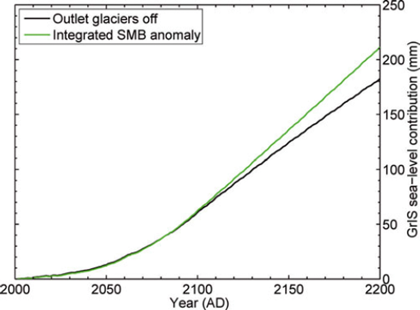
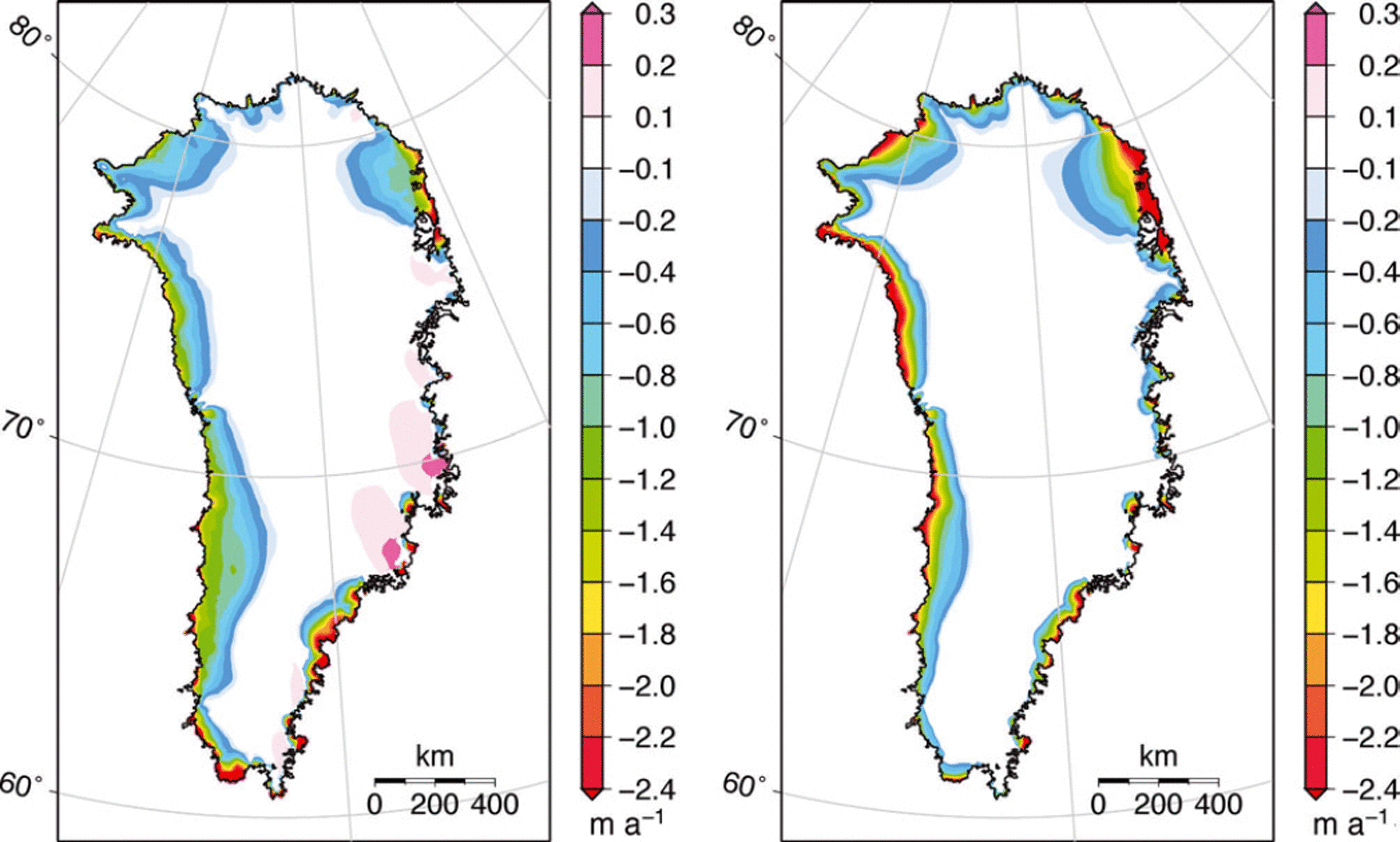
Figure 11 shows the thinning pattern after 200 years. The magnitude of the total thinning by ad 2200 amounts to up to 1000 m at the margin and is still >1 m at the ice divide upstream of JKB and HH. The inland propagation occurs mainly by geometric adjustment and therefore diffuses almost radially from the initial point of perturbation (cf. Reference Fürst, Rybak, Goelzer, De Smedt, de Groen and HuybrechtsFürst and others, 2011). These radial patterns are very similar across all model resolutions tested, suggesting that the effect of glacial channelling at the ice-sheet margin does not have a significant influence.

Fig. 11.

Ice-thickness changes by ad 2200 compared to ad 2000 due to outlet glacier retreat.

An additional experiment, in which only the four explicitly modelled glaciers are considered without further SMB feedbacks, brought to light that simulated fluxes are largely comparable between the flowline and large-scale models (Fig. 12) except for KNG, as discussed above. For a better comparison, the constant mass loss by synthetic SMB correction is added as an offset to the flux of KNG and HH (dashed line in Fig. 12b). The episodic and rapid increase of fluxes in the large-scale model is caused by loss of entire gridcells while the grounding line can retreat more gradually in the flowline model.

Fig. 12.

Comparison of grounding line fluxes between (a) flowline model and (b) large-scale model. (a) is produced with data from Reference NickNick and others (2013) for the applied medium scenario. Dashed lines in (b) result from adding the mass loss by synthetic SMB correction to the simulated fluxes of KNG and HH.

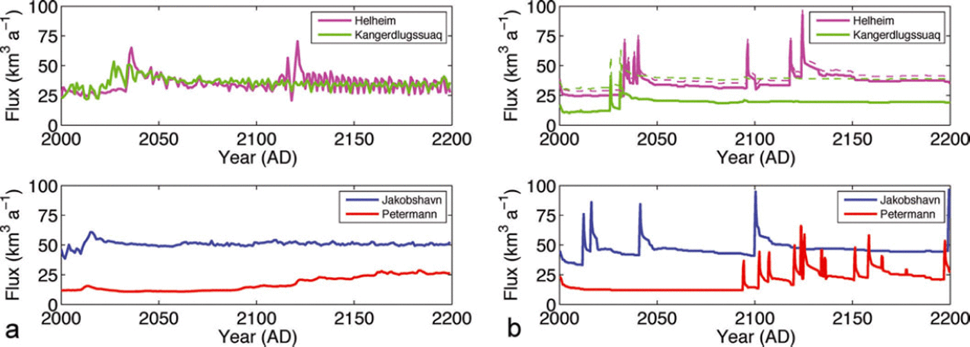
Despite differences in modelling of two and three dimensions, the retreat of the glaciers in the large-scale model, most important for the large-scale response, is (by construction) in good agreement with that simulated by the flowline model. Dynamic sea-level contributions by ad 2200 are somewhat larger in the large-scale model for JKB (7.1 mm) and PTMN (3.5 mm) compared to the dynamic contributions from the flowline model (6.6 and 2.9 mm) of Reference NickNick and others (2013). The large-scale response includes a 3-D thinning propagation in addition to the prescribed retreat and thinning rates at the margin. The 3-D flow reacts as a diffusive thinning wave that is transmitted inland in direct response to a steeper margin.

The dynamic sea-level contributions for HH (4.4 mm) and KNG (1.2 mm) are lower than the flowline model results of 6.1 and 4.3 mm, representing low biases in relative terms of 28% and 72%, respectively. These are similar to the relative amount of flux exported by the synthetic SMB correction for these glaciers (Table 1), which is quasi-constant in time and does not contribute to the dynamic response. To correct for these biases relative to the flowline model results, sea-level contributions for the four glaciers combined would have to be increased by 20%. JKB and PTMN serve for the majority of the generalization, which accounts for on average 50% of the entire mass loss induced by outlet glacier forcing. To cover the additional uncertainty in how far biases for the four glaciers are representative, we increase the lower and upper bound for dynamic contributions including the generalization by 10% and 20%, respectively. The updated range of outlet glacier contributions to sea-level rise is then 8–18 mm at ad 2100 and 13–38 mm by ad 2200.

6.3. Basal lubrication

Including the contribution from enhanced basal lubrication adds only 0.8 mm to the projected sea-level contribution in our reference run. The effect is negligible compared to SMB changes, as shown for a wider range of ice-sheet models and relations between runoff and speed-up in Shannon and others (in press). There appear to be three main reasons for the limited effect. Much of the perimeter of the GrIS is land-based, and here accelerated flow only generates a displacement but not a loss of the ice. This limits the potential effect on sea-level change mainly to marine-terminated margins. But there the process is already active for the present day, and beyond a certain surface melt rate the ice decelerates rather than accelerates. A net marginal deceleration is the reason for negative sea-level contributions for some runoff–speed-up relations in Shannon and others (in press). Finally, there is an additional feedback of meltwater lubrication on SMB changes. As ice is accelerated towards the margin, it increases the surface elevation and increases the SMB there. This effect partially compensates the drawdown of the surface at higher elevations, with an effect of the opposite sign.

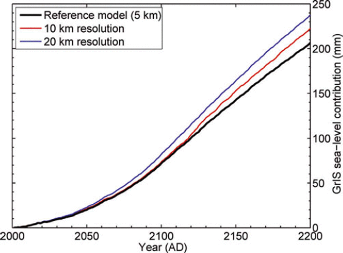
6.4. Horizontal ice-sheet model resolution

To evaluate dependence of the projections on the ice-sheet model resolution, additional experiments were performed on 10 and 20 km grids. The results are shown in Figure 13 for otherwise the same modelling strategies as in the reference experiment. Overall, the GrIS sea-level contribution increases with decreasing model resolution. The associated increases amount to 16 mm (10 km) and 31 mm (20 km) after 200 years. Since these experiments all apply the same MAR-SMB anomalies, the resolution dependence must be due to some aspects of the ice-dynamic model. It appears to be mainly related to the synthetic SMB corrections required for initialization, which are larger for lower-resolution models where outlet glaciers are less well resolved. The bulk of the corrections account for limited ice discharge at marine-terminated margins. While intrinsically simulated discharge decreases over the course of the experiments in a similar way, the corrections are held constant in time and contribute to a larger sea-level response for lower-resolution models. Thinning of affected marine margins is to a minor extent further amplified by the height–SMB feedback. Another (minor) effect is that prescribed outlet glacier retreat is implemented in the model as removal of full gridcells, which leads to a larger contribution in lower-resolution models.

Fig. 13.

Effect of horizontal ice-sheet model resolution on the projected ice-sheet evolution.

6.5. Initialization with freely evolving geometry

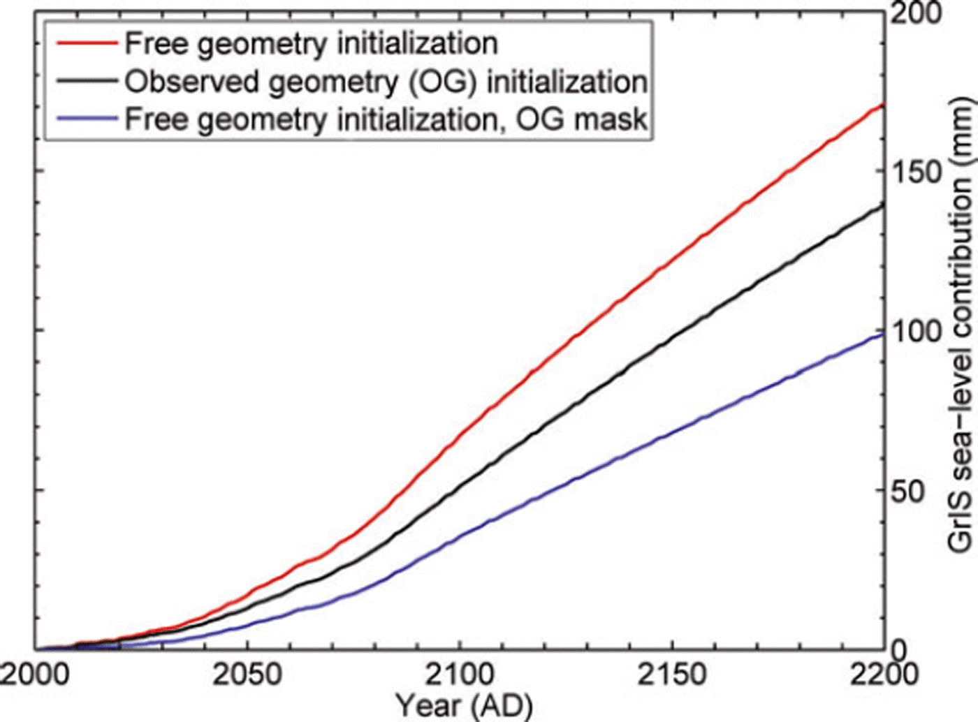
Finally, we also investigated the effect of the initialization technique. Using a freely evolving ice sheet (FG: free geometry) resulting from a glacial–interglacial spin-up procedure as an initial condition (Reference Graversen, Drijfhout, Hazeleger, Van de Wal, Bintanja and HelsenGraversen and others, 2011; Reference Greve, Saito and Abe-OuchiGreve and others, 2011) has the advantage of being fully self-consistent, albeit with the shortcoming that the ice-sheet geometry is not as close to the observations as the reference initialization from observed geometry (OG). A quantitative comparison between the two initialization techniques is limited owing to these differences in ice-sheet geometry, because they feed back on all other variables. A larger ice-sheet area in FG prevents the use of RCM forcing and the application of comparable prescribed outlet glacier retreat rates and basal lubrication. The comparison is therefore done with the same GCM-PDD forcing, only taking SMB changes into account, without outlet glacier dynamics and basal lubrication.

For the FG set-up, we obtain a projected sea-level rise of 171 mm by ad 2200, 22% larger than the 140 mm projected with the OG model (Fig. 14). This is mainly due to the larger size of the ablation area in the FG set-up. Correcting for different surface areas is, however, not straightforward, as illustrated by additionally showing volume changes with the FG model within the OG ice mask. In that case, the projected sea-level change would be 29% lower, as a large part of the FG ablation zone lies outside the OG mask. Projections based on a FG set-up (Reference Huybrechts and de WoldeHuybrechts and de Wolde, 1999; Reference Graversen, Drijfhout, Hazeleger, Van de Wal, Bintanja and HelsenGraversen and others, 2011; Reference Greve, Saito and Abe-OuchiGreve and others, 2011) do not routinely correct for area deviations, and therefore introduce an unquantified bias.

Fig. 14.

Comparison of Greenland sea-level contributions for two different initialization techniques.