

Introduction
For decades, protein chemists showed little interest in the unfolded state of proteins for several reasons. First, a central paradigm of protein biochemistry stipulates that proteins have to adopt a well-defined structure in order to perform their function. Based on Anfinsen’s early work, the respective structure was thought to be determined by its amino acid residue sequence and the solvent conditions (e.g., pH, temperature, ionic strength) (Anfinsen, Reference Anfinsen1973). Second, the unfolded or denatured state was considered as a random ensemble of protein conformations in which individual residues sample all sterically allowed regions of the Ramachandran plot as visualized in Figure 1 (Brant and Flory, Reference Brant and Flory1965a, Reference Brant and Flory1965b). Even the relatively recent energy landscape model of Wolynes and coworkers (Onuchi et al., Reference Onuchi1997; Ferreiro et al., Reference Ferreiro2014), which provides a rather complex physical picture of the folding process, generally assumes that unfolded proteins are describable as a residue-independent random coil-like ensemble. An ideal self-avoiding random coil ensemble does not contain any regular secondary structure sections. Its intrinsic dynamics are considered as a superposition of independent residue motions involving fluctuations along backbone and side chain dihedral angles (isolated pair hypothesis) (Flory, Reference Flory1953).
Upper panel: Resonance Structure of the peptide group (left) and Ramachandran plot based on dihedral backbone angles in folded proteins (right). The dihedral angles φ and ψ are defined by the positions of C’NCα C’ and NCα C’N, respectively (https://commons.wikimedia.org/wiki/File:Ramachandran_plot_general_100K.jpg). Lower panel: Ramachandran plots of the central residue of the cationic tripeptides GAG (left) and GVG (right) obtained from vibrational spectroscopy and NMR data (Hagarman et al., Reference Hagarman2010). The plots were created with a MATLAB program by the author.

Over the last three decades, these paradigms have faced significant challenges from experimental observations. Most importantly, the discovery of intrinsically disordered proteins (IDPs) revealed that a well-defined structure is not a prerequisite for biological function. These proteins perform a plethora of biological functions mostly in cellular contexts. Additionally, intrinsically disordered regions (IDRs) within otherwise folded proteins participate in pivotal protein–DNA and ligand–receptor interactions (Dunker et al., Reference Dunker2002, Reference Dunker2005; Uversky et al., Reference Uversky2008; Uversky, Reference Uversky2012; Holehouse and Kragelund, Reference Holehouse and Kragelund2024; Liu et al., Reference Liu2025). IDPs and IDRs are quite frequently found in eukaryotes, where between 30% and 40% of the residues are located in disordered regions (Deiana et al., Reference Deiana2019). The conformational flexibility of IDPs enables them to perform different functions, depending on their biological environment.
The classification of IDPs and IDRs shown in Figure 2 visualizes their functional diversity (Tompa, Reference Tompa2005). Entropic chains, for instance, function as springs and linkers such as the PEVK domain of titin, which provides a passive force in muscles (Linke et al., Reference Linke2002). All proteins of the second class shown in Figure 2 are involved in molecular recognition via their binding to other biological molecules (proteins, RNA, and DNA). Such interactions involve both permanent and transient binding (Dunker and Obradovic, Reference Dunker and Obradovic2001; Dunker et al., Reference Dunker2005; Uversky et al., Reference Uversky2005; Mohan et al., Reference Mohan2006; Oldfield et al., Reference Oldfield2008). Frequently, the recognition process induces a disorder-to-order transition (Dyson and Wright, Reference Dyson and Wright2005; Wright and Dyson, Reference Wright and Dyson2015). Regarding the latter, so-called short linear motifs (SLiMs) can frequently act as targeting signals, modifications, and ligand binding sites (Neduva and Russell, Reference Neduva and Russell2005, Reference Neduva and Russell2006; Kliche and Ivarsson, Reference Kliche and Ivarsson2022). The structural versatility and the ability of rather fast structural conversion facilitate the capability of IDPs to get involved in multivalent binding, binding to multiple partners, and to produce binding products with rather different dynamic properties (i.e., different degrees of fuzziness) (Oldfield et al., Reference Oldfield2008; Hsu et al., Reference Hsu2013; Wright and Dyson, Reference Wright and Dyson2015).
Functional classification scheme of intrinsically disordered regions. The function of IDRs stems either directly from their capacity to fluctuate freely about a large configurational space (entropic chain functions) or their ability to transiently or permanently bind partner molecule(s). For each functional class, a short description of the function is provided. Taken in modified from Tompa (Reference Tompa2005) with permission. Copyright (2005) Wiley & Sons.

Some IDPs are of great biomedical relevance in that they are prone to self-assembly into amyloid fibrils. The amyloid β -peptides Aβ1–40 and Aβ1–42, the human islet polypeptide, α-synuclein, and the tau protein are prominent representatives of this type of IDPs (Avni et al., Reference Avni2019; Carton and Buchete, Reference Carton and Buchete2025). Moreover, IDPs as well as partially folded proteins with IDRs in water can undergo liquid–liquid demixing processes, which lead to the formation of membrane-less organelles (Martin and Mittag, Reference Martin and Mittag2018; Borcherds et al., Reference Borcherds2021).
The multitude of IDPs and IDRs in nature reveals that the classical function–structure paradigm that guided the thinking of biochemists for a long period of time has to be revisited and extended. The frequent occurrence of IDRs in otherwise folded proteins suggests a continuum of structures, which reaches from fully folded to totally disordered proteins (IDPs with residual structure are counted toward the latter). Obviously, protein dynamics increase along this coordinate. While protein folding aims at minimizing frustration (Ferreiro et al., Reference Ferreiro2014), it is maximized in IDPs. Therefore, Holehouse and Kragelund replaced the classical structure–function paradigm with a sequence–ensemble–function relationship, which applies to all types of proteins.(Holehouse and Kragelund, Reference Holehouse and Kragelund2024). In folded proteins, the ensemble is reduced to taxonomic conformational substates, in which the protein performs the same function, though with different rates (Frauenfelder et al., Reference Frauenfelder1988). In IDPs, the much higher conformational diversity allows for a multitude of functions. The extent of conformational heterogeneity is, of course, dictated by the primary sequence, structural context, and solvent conditions.
IDPs and IDRs contain by far more charged and polar residues than foldable proteins (Uversky et al., Reference Uversky2000; Dunker et al., Reference Dunker2008; Habchi et al., Reference Habchi2014). This is not unexpected, since a dominance of residues with hydrophilic side chains would favor more extended protein structures in which these groups would become fully solvated. However, as demonstrated in Chapter 4 of this article, the relationship between charges and sampled protein conformations is more complicated than one would expect if one solely used the overall hydrophilicity of a protein as an indicator. Here, we just note that structurally, conformational ensembles of IDPs resemble the ones of unfolded proteins, namely pre-molten globules, molten globules, and more extended coils (Uversky, Reference Uversky2002). The latter are frequently described as random coils. This classical view assumes that locally individual amino acid residues sample the entire sterically allowed regions of the Ramachandran plot (Ramachandran et al., Reference Ramachandran1963; Ramakrishnan and Ramachandran, Reference Ramakrishnan and Ramachandran1965; Ramachandran and Sasisekharan, Reference Ramachandran and Sasisekharan1968; Pal and Chakrabarti, Reference Pal and Chakrabarti2002) and that, with the exception of glycine and proline, the Ramachandran distributions of residues with different side chains do not differ significantly. However, over the last three decades, results from experimental and computational analyses of ultrashort peptides in water (Avbelj et al., Reference Avbelj2006; Shi et al., Reference Shi2006; Schweitzer-Stenner, Reference Schweitzer-Stenner2023), and of coil libraries (Fitzkee et al., Reference Fitzkee2005; Jha et al., Reference Jha2005b; Ting et al., Reference Ting2010; Shen et al., Reference Shen2018) as well as from NMR studies (Jensen et al., Reference Jensen2014) of unfolded foldable proteins and IDPs challenged this view. The new view that emerged from these studies is demonstrated by the Ramachandran plots of the central residues of (cationic) GAG and GVG in water shown in Figure 1, which were obtained from spectroscopic studies on GxG peptides (x: host residue) in solution (Hagarman et al., Reference Hagarman2010). Contrary to text book plots for the alanine dipeptides in the classical papers of Ramachandran (Ramakrishnan and Ramachandran, Reference Ramakrishnan and Ramachandran1965; Ramachandran and Sasisekharan, Reference Ramachandran and Sasisekharan1968), Flory (Brant and Flory, Reference Brant and Flory1965a) and later works (Ho et al., Reference Ho2003; Mironov et al., Reference Mironov2019), alanine predominantly samples a space which is assignable to polyproline II (pPII) structures. Sampling of other classical secondary structures (β-strand and right-handed helices) is by far less pronounced. pPII is a conformation adopted by trans-poly-L-proline peptide segments (Cowan and Mc Gavin, Reference Cowan and Mc Gavin1955) or by proteins with PG and PHypG repeat sequences (e.g., collagen) (Matsushima et al., Reference Matsushima2008; Shoulders and Raines, Reference Shoulders and Raines2009). The situation is significantly different for valine. Its Ramachandran plots suggest a similar sampling of pPII and β-strand. For both amino acid residues, helical and turn structures display much lesser populations, a clear departure from the significant helical fractions to be found in older Ramachandran plots (cf. Figure 1). The backbone populations indicated in Figure 1 reveal side chain specificity and, compared with classical plots, a reduced conformational space, which implies a reduced configurational entropy (Schweitzer-Stenner and Toal, Reference Schweitzer-Stenner and Toal2014). Side chain dependencies of Ramachandran plots and high pPII propensity of alanine also emerged from the analysis of coil libraries (Zaman et al., Reference Zaman2003; Shen and Bax, Reference Shen and Bax2007; Jiang et al., Reference Jiang2010; Ting et al., Reference Ting2010; Debartolo et al., Reference Debartolo and Schweitzer-Stenner2012). It is obvious that with such residue-dependent conformational propensities, protein conformations of unfolded and extended intrinsically disordered proteins cannot be nearly isoenergetic. Thus, a totally unfolded polypeptide or protein is locally better described as a statistical coil, as suggested by the late Harold Scheraga and his colleagues (Tanaka and Scheraga, Reference Tanaka and Scheraga1976).
Replacing the random coil view of unfolded proteins with the more general statistical coil concept is an important but still quantitative rather than qualitative change. As a random coil, a statistical coil does not contain any defined secondary residual structure. However, multiple lines of evidence, mostly from comprehensive NMR studies, revealed that such residual structures in fact appear in IDPs (Wells et al., Reference Wells2008; Cho et al., Reference Cho2009; Ozenne et al., Reference Ozenne2012; Jensen et al., Reference Jensen2014; Schwalbe et al., Reference Schwalbe2014). As a representative example, Figure 3 shows the secondary chemical shift of the signal assignable to the 13Cα atoms of the disordered C-terminal of the measles virus nucleoprotein (N-tail) alone and in a complex with the phosphoprotein PXD (Jensen et al., Reference Jensen2011). A secondary shift is calculated as the difference between a measured chemical shift and a residue specific value obtained from the NMR spectra of short host–guest peptides that is considered to represent a statistical coil (Braun et al., Reference Braun1994; Bundi and Wüthrich, Reference Bundi and Wüthrich1979; Kjaergaard and Poulsen, Reference Kjaergaard and Poulsen2011; Wishart et al., Reference Wishart1995; Wishart et al., Reference Wishart1995; Wishart and Nip, Reference Wishart and Nip1998; Wishart and Sykes, Reference Wishart and Sykes1994). The secondary shifts of N-tail in Figure 3 suggest that a substantial number of residues sample backbone distributions differ from the respective local statistical coil distributions. The rather systematic positive shifts in the region around residue 100 are indicative of the transient formation of right-handed helices. The more scattered secondary shifts of other residues might reflect specific nearest- and second-nearest-neighbor interactions between residues (Schweitzer-Stenner and Toal, Reference Schweitzer-Stenner and Toal2016), which are neglected in the classical random coil model (isolated pair hypothesis, IPH). For the above NMR analysis, nearest-neighbor interactions are generally inferred from the influence of neighbors on the chemical shift of glycine or glutamate (Kjaergaard and Poulsen, Reference Kjaergaard and Poulsen2011). Thus, it is assumed that it does not depend on the side chain of the target.
Secondary chemical shifts of the 13Cα atoms of N Tail alone (blue bars) and in complex with the α-helical C-terminal domain of the phosphoprotein (PXD; red bars) with respect to a statistical coil chemical shift standard. In the free form, the values for the region encompassing the residues 90–110 (red bars) are shifted downfield, indicating a transiently populated right-handed α-helix in the presence of PXD. Taken with permission from (Jensen et al., Reference Jensen2011).

The above-discussed local conformational propensities of amino acids are solely relevant for totally unfolded IDPs and IDRs. However, as indicated above, this condition is not always met since both can exist globally as molten globule, pre-molten globule, and statistical coil ensembles. They can be distinguished in terms of the exponent ν of Flory’s scaling law for, for example, the radius of gyration Rg, namely:
 $$ {R}_g=A{N}^{\nu }, $$
where A is a constant, and N is the number of residues. Rg can be determined experimentally by small-angle X-ray scattering (SAXS) measurements and computationally by molecular dynamics (MD) simulations (Zheng and Best, Reference Zheng and Best2018; Mugnai et al., Reference Mugnai2025). Only unfolded or disordered coils describable by a Flory exponent close to 0.6 are described as (global) self-avoiding random coil (Flory, Reference Flory1953). In principle, an exponent of 0.5 is indicative of an ideal Gaussian chain, but such a scenario is unrealistic because of excluded volume effects. Hence, ν values lower than 0.6 reflect different degrees of compactness. Under certain conditions discussed in Chapter 4, the exponent can even exceed this threshold, thus representing an extended statistical coil.
Other metrics such as hydrodynamic radii, end-to-end distances, and average distances between residues follow similar scaling laws with the same exponents for random coil distributions (Mao et al., Reference Mao2010; Waszkiewicz et al., Reference Waszkiewicz2024). Long-range distance distributions between fluorescently labeled residues can be determined by fluorescence energy transfer measurements (Hofmann et al., Reference Hofmann2012). An alternative option to distance distributions is asphericity. It is defined as:
 $$ \Delta =\frac{3}{2}\frac{\sum \limits_1^3{\left({\lambda}_i-\overline{\lambda}\right)}^2}{( tr\hat{T}\Big)}, $$
where $ \overline{T} $
is the inertia tensor, λi its eigenvalues, and
$ \overline{T} $
is the inertia tensor, λi its eigenvalues, and $ \overline{\lambda} $
reads as the trace of the tensor divided by 3 (Dima and Thirumalai, Reference Dima and Thirumalai2004). Apparently, it is zero for a perfect sphere and maximal for a perfect rod. For an ideal random coil (polymer in a theta solvent), it is 0.39 and 0.43 for a self-avoiding random coil (Mao et al., Reference Mao2010).
$ \overline{\lambda} $
reads as the trace of the tensor divided by 3 (Dima and Thirumalai, Reference Dima and Thirumalai2004). Apparently, it is zero for a perfect sphere and maximal for a perfect rod. For an ideal random coil (polymer in a theta solvent), it is 0.39 and 0.43 for a self-avoiding random coil (Mao et al., Reference Mao2010).
This review focuses on IDPs and IDRs that, in the absence of binding and self-assembly, are describable as a statistical coil with and without transient secondary structures. This encompasses proteins with a Flory exponent larger than 0.5 (theta point). Locally, such IDPs are likely to deviate from the local random coil behavior (vide supra). Globally, however, they can behave like a self-avoiding random coil with Flory exponents close to 0.6 (Fitzkee and Rose, Reference Fitzkee and Rose2004; Jha et al., Reference Jha2005a). Several questions are posed by the above results that all focus on the role of water. It is well known that the dominance of intramolecular over protein–solvent interactions promotes the folding of proteins. In an unfolded statistical coil, adopting protein–solvent interactions can be expected to dominate. Therefore, the question arises to what extent peptide/protein–water interactions affect the structural thermodynamics (conformational propensities of residues and residual structure formation) and conformational dynamics of IDPs. Moreover, since the strength of IDP–water interactions determines the solubility of the former, it is of relevance for an understanding of protein aggregation into amorphous aggregates, which can develop into amyloid fibrils or serve as a starting point for liquid–liquid demixing into liquid droplets.
This review article aims to provide a comprehensive overview of all aspects of peptide/protein solvation in the unfolded state, with a strong emphasis on intrinsically disordered proteins and protein segments. It asks to what extent protein-water interactions determine the thermodynamics of local backbone distributions. It addresses the question of the extent to which the dominance of charged and polar residues facilitates interactions with water and stabilizes statistical coil states. Furthermore, it explores to what extent the structure and dynamics of hydration water of IDPs differ from those of folded proteins in a qualitative way. For the latter, several lines of experiments have led to a complex and still not completed picture of the interplay between water and protein dynamics, which is pivotal for its function (Ball, Reference Ball2008; Schirò et al., Reference Schirò2015). Much larger surface accessible areas and the dominance of hydrophilic residues in coiled IDPs make it likely that the coupling between hydration water and protein motions differs from that in folded proteins. Finally, the article explores the role of water in the formation of droplets involving IDPs.
This article is organized as follows. In order to put the discussion of the interplay between protein disorder and solvation into a broader context, the second chapter briefly discusses the properties of hydration water and its influence on folded proteins as a kind of benchmark system. It provides a brief overview of different concepts aimed at describing the stabilizing influence of water on folded proteins as well as the possible functional relevance of water dynamics in the hydration shell. The third chapter focuses on how the free energy landscape of amino acid residues in short peptides is related to site chain-specific residue hydration. They are frequently used as convenient model systems for an exploration of the local conformational dynamics of IDP residues. I describe experimental and computational studies that invoke hydration as the dominant cause for side chain specificity of conformational propensities, which leads to a deviation from the frequently assumed local random coil behavior (vide supra). In this context, I also discuss studies that explored the influence of cosolvents (glycerol, ethanol, etc.) on peptide conformations. The fourth chapter covers experiments and theoretical studies on how the interplay between solvation, charge distribution (of the peptide or protein), ionic strength, and temperature decides whether an IDP adopts a molten globule, pre-molten globule, or coil state. While the peptide studies described in Chapter 3 explore local aspects of unfolded systems, the studies described in Chapter 4 focus more on the above-introduced determinants of their global state. Additionally, this chapter presents the results of some spectroscopic and computational studies that explored structural and dynamic aspects of the hydration shells of IDPs and related coupling between water and protein motions. Chapter 5 looks at the role of water in facilitating or impeding the self-assembly of IDPs into droplets via liquid–liquid demixing. The article closes with a summary of takeaway points and an outlook.
Owing to its focus on IDP hydration, this article discusses structural and specific functional aspects of IDPs only in passing (mostly in Chapter 3). There are several extensive reviews available for readers who are interested in these aspects (Uversky et al., Reference Uversky2008; Uversky, Reference Uversky2013; Habchi et al., Reference Habchi2014; Jakob et al., Reference Jakob2014; Jensen et al., Reference Jensen2014; Uversky et al., Reference Uversky2014; Schweitzer-Stenner, Reference Schweitzer-Stenner2023; Schweitzer-Stenner, Reference Schweitzer-Stenner2025). For a more general overview, the reader is referred to the very recent, excellent article of Holehouse and Kragelund (Reference Holehouse and Kragelund2024). In what follows, I solely use the acronym IDP if general properties of IDPs and IDRs are discussed. The term IDR is only used if the text deals explicitly with a specific disordered region.
Protein stability and dynamics in water
Introduction of the topic
Owing to the abundance of water in all forms of life on earth (Ball, Reference Ball2005), one is tempted to believe that water must be an ideal solvent for many proteins and polynucleotides. Interestingly, however, this notion is only half true. From a polymer physics point of view, water is not a good solvent for foldable proteins at room temperature, because this would require a dominance of protein–water over intramolecular protein interactions (Flory, Reference Flory1953; de Gennes, Reference de Gennes1979). However, the meaning of the term ‘good’ is relative in this context. If water were indeed a good solvent for all proteins, they would not fold at room or physiological temperature, because the vast majority of amino acid residues and the peptide groups would prefer interactions with water over any contact with other protein components. Apparently, this is not the case for foldable proteins.
Water is pivotal for the stability of many non-membrane proteins. Thermodynamically, it can promote folding via the so-called hydrophobic effect. The hydration shell of proteins is constituted by a highly flexible network of hydrogen-bonded water molecules, the dynamics of which are coupled to protein motions and vice versa. Hence, proteins and hydration shells should be understood as an entity. In this first section of this chapter, the thermodynamic aspects of protein–water interactions are discussed. In this context, conflicting views on the role of hydrogen bonding are elucidated. The second and third section presents some representative work on hydration and protein dynamics explored by dielectric, terahertz, fluorescence, IR, and NMR spectroscopy. Conflicting results reveal that a comprehensive and consistent understanding of the interplay between water and protein motions is an ongoing project.
Water and protein folding
Why do certain polypeptides try to avoid water at least partially and fold into relatively compact structures? In attempts to answer these questions, two schools of thought have emerged in the last century. Initially, the understanding of protein folding was dominated by Pauling’s emphasis on intramolecular, inter-peptide hydrogen bonding between amide and carbonyl bonds of different peptide groups. The strength of such hydrogen bonds was estimated to be of the order of −8 kJ/mol (Pauling et al., Reference Pauling1951). Such a model seemed to be entirely plausible since regular secondary structures like right-handed helices and β-sheets involve a very ordered set of exactly this type of hydrogen bonding, which stabilizes backbone structures in the sterically permissible region of the Ramachandran plot. Later developed statistical thermodynamics models of coil to helix transitions provided a plausible rationale for intra-backbone hydrogen bonding to be the source of the cooperativity observed for the formation of helical secondary structures (Zimm and Bragg, Reference Zimm and Bragg1959; Lifson and Roig, Reference Lifson and Roig1961). The model of Pauling and coworkers did not consider any side chain specificity for secondary structure formation. The latter was thought to be relevant solely for the formation of tertiary structures.
In spite of its plausibility, the acceptance of the backbone emphasizing the Pauling model did not last long. Theoretically, the lack of dominance of backbone–backbone over backbone–water hydrogen bonding was rationalized by Fersht’s inventory argument (Figure 4; Fersht, Reference Fersht1987). Here, Pr and Pr’ symbolize two peptide groups. Pr accepts a hydrogen bond from two water molecules and Pr’ donates one to a water molecule. A simple accounting exercise shows that when two peptide groups form an intramolecular hydrogen bond, they must break their existing hydrogen bonds with water. The key insight is that no new hydrogen bonds are created overall – the system merely reorganizes from three peptide–water bonds to one peptide–peptide bond plus three new water–water bonds. Since all hydrogen bonds have similar energies, the net energetic change is minimal, explaining why intramolecular hydrogen bonding provides little driving force for protein folding. The incapability of intramolecular hydrogen bonding to compete with backbone–water hydrogen bonding formation was corroborated by thermodynamic experiments that explored the self-assembly of N’-methylacetamide in different solvents, including water (Klotz and Franzen, Reference Klotz and Franzen1962; Schweitzer-Stenner et al., Reference Schweitzer-Stenner1998).
Schematic representation of the inventory argument. In the separated state, the NH group on one peptide and the CO group of another form a total of three hydrogen bonds with water. Upon dimerization, they are replaced by a single intermolecular bond between the CO and NH group of the interaction peptides and two water–water bonds. Even if one expects that all hydrogen bonds have similar bonding energies, the gain for dimerization should be minimal.

The need for an alternative explanation was met by the hydrophobic interaction model (Kauzmann, Reference Kauzmann1956, Reference Kauzmann1959). It predicts that the dehydration of aliphatic and aromatic groups contributes significantly to the stability of a folded protein. The details of his thermodynamic concepts are textbook knowledge. Here, we just briefly summarize the different contributions of side chain hydration to the total Gibbs free energy of hydration at different temperatures. If we associate the hydrated and dehydrated side chain with the unfolded and folded state, respectively, a negative free energy ΔGh,uf = Gu–Gf indicates a stabilizing contribution to the unfolded, hydrated state of a protein. Figure 5 displays the representative changes of the heat capacity, enthalpy, entropy, and Gibbs free energy of aliphatic and aromatic model compounds, all normalized on the respective solvent accessible surface as a function of temperature. In addition, corresponding data for the glutamic acid side chain, as a representative of ionized groups, are plotted. The solid lines therein connect data points taken from the literature (Makhatadze and Privalov, Reference Makhatadze and Privalov1995). The Gibbs free energy of aliphatic groups is positive over the entire temperature range. Hence, they favor the folded state. The enthalpic contribution is negative below 90 °C and positive above, which indicates that the unfolded state is favored over the folded one at room temperature. However, this is overcompensated by the negative entropy contribution to the Gibbs energy, which clearly favors the folded state until it reaches zero above 100 °C. The heat capacity change exhibits only a modest change with temperature. The traditional interpretation of the data in Figure 5 by Kauzmann invokes a scenario where water forms a cage-like structure around an aliphatic group, which is enthalpically favored but entropically disfavored compared with the much higher mobility of the involved water molecules in the bulk. Hence, the avoidance of water by hydrophobic groups is entropic in nature at room temperature. A modified version involving the ordering of water molecules around aliphatic groups by van der Waals interactions has more recently been proposed (Baldwin, Reference Baldwin2014). The Gibbs free energy of glutamic acid (representing ionized groups) is negative and clearly favors the unfolded state because of its strong interaction with water. This enthalpic stabilization cannot be compensated for by the reduction of entropy. Enthalpy and entropy depend only slightly on temperature. Aromatic groups exhibit a modest preference for the unfolded state. An entropy–enthalpy compensation leads to a nearly temperature-independent Gibbs free energy. Taken together, the data in Figure 5 suggest that with regard to hydration, the folded state is solely stabilized by the entropic contribution of aliphatic group hydration at room temperature. Of course, solute–solvent and solute–solute hydrogen bonding and van der Waals interactions, as well as changes of the configurational entropy, have to be added to the Gibbs energy balance. The proposed propensity of aliphatic groups to become buried in the protein interior is supported by an analysis of 218 proteins, in which aliphatic and aromatic residues were found to be buried, on average, by 75% (Malleshappa Gowder et al., Reference Malleshappa Gowder2014).
Normalized values (per nm2 of the surface accessible area) of heat capacity, enthalpy, entropy, and Gibbs energy of hydration for side chain surfaces plotted as a function of temperature: aliphatic groups (blue, aromatic groups (red), and glutamic acid (yellow) as representatives of charged and polar groups. The solid lines in the figures connect experimental data measured at 5, 25, 50, 75, 100, and 125 °C. The data were taken from Table 4 in the paper of Makhatadze and Privalov (Reference Makhatadze and Privalov1995). The figure was produced with a MATLAB program.

While the hydrophobic effect is still considered the major driving force of protein folding, its dominance over intramolecular hydrogen bonding has not remained unchallenged. For a long period of time, it has been believed that only very long polypeptides can undergo a coil > helix transition (Epand and Scheraga, Reference Epand and Scheraga1968), since peptide segments resembling helical segments in proteins would remain unfolded in isolation. However, this view was challenged by experiments that revealed the capability of (partial) helix formation of the 13-residue C-peptide from the N-terminus of ribonuclease A and of a multitude of alanine-based peptides with fewer than 20 residues (Brown and Klee, Reference Brown and Klee1971; Scholtz and Baldwin, Reference Scholtz and Baldwin1992; Baldwin, Reference Baldwin1995). The thermal unfolding/folding of these oligopeptides could be modeled with modified versions of the classical Zimm–Bragg or Lifson–Roig theory (Qian and Schellman, Reference Qian and Schellman1992). Subsequently, the relevance of intramolecular hydrogen bonding, including the potential role of water bridges for protein folding, has been emphasized by many researchers based on experimental and theoretical insights. The interested reader is referred to a multitude of conceptual and review articles for more details (Ben-Naim, Reference Ben-Naim1991; Scholtz and Baldwin, Reference Scholtz and Baldwin1992; Rose, Reference Rose1997; Baldwin, Reference Baldwin2007; Rose, Reference Rose2021). Here, we just refer to a feature article (Baldwin and Rose, Reference Baldwin and Rose1999), which divides foldable proteins into two classes. Class I (e.g., apo-myoglobin, RNase H, cytochrome c) folds hierarchically in that secondary structure is formed first and is subsequently stabilized in molten globule intermediates. Class II proteins undergo a two-state process (e.g., chymotrypsin inhibitor, cold-shock protein B) that starts with tertiary nucleation. Altogether, one can currently state that at room temperature, water is a poor solvent for the unfolded state of foldable proteins, but a good solvent for the folded protein. The exact mechanism of the folding process depends on the amino acid residue sequence and the respective propensities for distinct secondary structures, as well as on environmental parameters such as pH, ionic strength, and temperature.
One yet unmentioned and not fully understood aspect of water–protein interactions should be mentioned here, since it is also of interest for understanding disordered peptides and proteins (Chapters 3 and 4). Generally, estimations of the contribution of backbone and side chain desolvation are based on the assumption of additivity. In other words, the solvation free energies of individual side chains and peptide groups obtained from organic analogues (Wolfenden et al., Reference Wolfenden1981; Kyte and Doolittle, Reference Kyte and Doolittle1982) and model peptides can just be added up to yield the total solvation/desolvation free energy of a folding process (Dill, Reference Dill1997). However, theoretical considerations by Ben Naim suggest that the solvation of the side chain and backbone is not independent (Ben-Naim, Reference Ben-Naim2011). Experiments by Della Gatta et al. (Reference Della Gatta2006) and theoretical analyses by Avbelj and Baldwin (Reference Avbelj and Baldwin2004) and by König and Boresch (Reference König and Boresch2009) and König et al. (Reference König2013) provide strong evidence for the invalidity of the group additivity concept. The latter researchers surmised that the apparent success of the method (i.e., its ability to reproduce experimental solvation free energies of proteins) might be due to a cancellation of errors.
Water dynamics in the hydration shell
In order to understand the interplay between protein and water in the hydration shell one has to address the following issues: (a) the thickness of the hydration shell, that is the sphere in which the properties of water differ from the one in the bulk, (b) the translational (self-diffusion), rotational and vibrational dynamics of solvation water and (c) the interplay between solvation water and protein dynamics and its relevance for protein function. Items (a) and (b) are addressed in this paragraph, while item (c) is the subject of paragraph 2.3.
The dynamics of water hydration have been studied experimentally and computationally. Experimental studies utilized time-resolved IR and fluorescence spectroscopy, broadband spectroscopy, NMR, and last but not least, terahertz (THz) spectroscopy. For the sake of brevity, I focus here on some very representative studies and refer the reader to the literature for a broader study of the subject (Dill et al., Reference Dill2005; Levy and Onuchic, Reference Levy and Onuchic2006; Laage et al., Reference Laage2012; Nibali and Havenith, Reference Nibali and Havenith2014; Laage et al., Reference Laage2017; Mieres-Perez et al., Reference Mieres-Perez2025).
Let us start with some aspects of water dynamics in the bulk, which can be described in terms of rotational, vibrational, and diffusive motions (Laage et al., Reference Laage2017). Figure 6 shows a representative structure of water, where the central molecule is coordinated by four other water molecules, forming two hydrogen bonds to O and receiving two from the OH groups. This hydrogen bonding network does not permit unhindered rotational and translational motions. Molecular rotation is replaced by a so-called hindered rotation or liberation mode around the principal axis. Results from computational studies by Petersen et al. suggest that upon excitation, this small-scale change predominantly transfers rotational energy to its neighbors in the hydration shell on a femtosecond time scale (Petersen et al., Reference Petersen2013; Laage et al., Reference Laage2017). Only a small fraction is used for translation. Of greater interest and relevance is a larger-scale collective motion that was originally suggested by Hynes and coworkers, namely a combined jump-reorientation motion (Laage et al., Reference Laage2012). Its basic aspects are also depicted in Figure 6. It involves first an elongation of a hydrogen bond upon the approach of an oxygen acceptor. Once the initial and the new acceptor have the same distance to the hydrogen atom of the rotating water molecule, the hydrogen bond switches between acceptors after the formation of a bifurcated transient state.
(a) Representation of water complexes in bulk water. The central water molecule is hydrogenbonded to four water molecules which constitute its first hydration shell. Molecules 1 and 2 are accept ing hydrogen bonds from the central H2O molecule, and molecules 3 and 4 are donating H-bonds to the central molecule. (b) The principal axes for a rigid rotor type H2O molecule. Taken from (Petersen et al., Reference Petersen2013) with permission. Copyright by the American Chemical Society 2013.

In a very recent study of Offei–Danso et al., the details of this combined rotational and jump motion were explored by molecular dynamics simulation (Offei-Danso et al., Reference Offei-Danso2023). They characterized the underlying dynamics by measuring the permanent dipole moment of water molecules with respect to a fixed coordinate system. Their results are illustrated in Figure 7, taken from their paper. On the left, the fraction of water molecules found to undergo reorientations by more than 60° are highlighted (a). The extent of their rotational changes is shown in the central images (b and c). The plots in the 7d show the oscillation of permanent dipole moments on a femtosecond time scale. The obtained results revealed further that dipole swings and the variation of defects (water with a lack of water coordination) are somewhat correlated. The observed angular jumps were found to involve highly cooperative motions of water molecules.
Representation of the collective nature of angular jumps in water. Left: Highlighted in red are all water molecules undergoing angular reorientation of magnitude greater than 60 degrees in a box of 3.2 nm within the time interval of 350 fs (which spans between time steps 1000 fs and 1350 fs in the MD simulation). They encompass an amount of around 5% of the total number of 1019 molecules used for the simulation. Middle: Zoom in on 8 of these molecules in a small region of the box at the start (b) and at the end (c) of a large angular jump as observed from the changes in their dipole vectors. The colored arcs outline the angular motion carried by the dipole vectors in the direction of the dashed arrow. Right: Change of the permanent dipole vector over time plotted with respect to one of the axes of the laboratory coordinate system for each of the selected molecules. For each molecule, the component that changes most in this time interval is shown. The regions between the start and the end of the angular jump are shaded by the colors of the corresponding molecules in panels b, c. Taken from Offei-Danso et al. (open source) Offei-Danso et al. (Reference Offei-Danso2023).

What happens with water in the vicinity of the protein surface? Generally, one can state that orientational motions are constrained owing to hydrogen bonding to backbone and side chain groups and the low-entropy solvation of aliphatic groups. This leads to higher water density, which can be probed by neutron scattering. Due to the rather different physical and steric properties of side chains, protein surfaces have a complex topography that gives rise to a heterogeneity in terms of a broad spectrum of rotational correlation times, which range from pico- to nanoseconds (Persson and Halle, Reference Persson and Halle2008).
For a long period of time, it was assumed that the thickness of the solvation shell of proteins amounts to about 3 Å (Svergun et al., Reference Svergun1998). This number was inferred from orientational correlation data. However, as Havenith and collaborators claimed, the number depends very much on the time window that an applied (spectroscopic) method uses. These researchers used terahertz (THz) spectroscopy as a tool to probe the vibrational dynamics of hydration water (Nibali and Havenith, Reference Nibali and Havenith2014). The insights gained by their work warrant a short account of the employed experimental method.
THz spectroscopy probes vibrations in the far-infrared regime. Figure 8 shows the experimental and calculated THz spectrum of water. Contrary to vibrational bands in classical IR spectra (1,000–3,500 cm−1), the bands are rather broad, which reflects the delocalized nature of the probed vibrations. Delocalization occurs through the hydrogen bonding network and electrostatic interactions between water molecules. The isotropic absorption coefficient for each mode can be calculated as a function of the total electronic dipole moment $ \overrightarrow{M} $
of volume V fluctuating with a frequency ω via the following Fourier transformation (Nibali and Havenith, Reference Nibali and Havenith2014):
$ \overrightarrow{M} $
of volume V fluctuating with a frequency ω via the following Fourier transformation (Nibali and Havenith, Reference Nibali and Havenith2014):
 $$ \alpha =F\left(\omega \right){\int}_0^{\infty }{e}^{\left( i\omega t\right)}\left\langle \overrightarrow{M}(0)\overrightarrow{M}(t)\right\rangle dt $$
Experimental terahertz absorption spectra of H2O (blue) and D2O (green) measured at 20 °C with Fourier transform spectroscopy compared to the ab initio molecular dynamics (AIMD) based H2O spectrum (red) obtained from Eq. (1). The thick red line shows smoothened AIMD data to guide the eye. In the upper inset, the full AIMD IR spectrum is compared to the standard experimental H2O spectrum. The change in absorbance of mixtures of light and heavy water with increasing mole fraction of heavy water at 20 °C is shown in the lower inset with respect to the pure water spectrum. The difference of the integrated THz absorption coefficient between 2.1 and 2.8 THz (centered at 2.4 THz) was measured as a function of the D2O fraction. Taken from Heyden et al. (Reference Heyden2010) with permission. Copyright by the National Academy of Sciences USA, 2010).

The frequency-dependent pre-factor is written as:
 $$ F\left(\omega \right)=\frac{1}{4\pi {\epsilon}_0}\frac{2\pi \beta {\omega}^2}{3 Vcn\left(\omega \right)}, $$
where c is the vacuum velocity of light and n is the frequency-dependent refractive index. The correlation function for the total dipole moment in Eq. (3) can be expressed as a sum over self- and cross-correlation functions of molecular dipoles (Heyden et al., Reference Heyden2010). The spectrum in Figure 8 contains only two broad maxima at 200 and 620 cm−1. The latter can be assigned to collective liberation modes introduced above. The former can be decomposed into contributions at 80, 160, 220, and 290 cm−1. The 80 cm−1 mode was assigned to a concerted motion in the second hydration shell. The remaining three wavenumbers represent coupled stretching modes of the first hydration shell, which represent different donor-acceptor topologies.
If the hydration water of proteins followed Beer–Lambert’s law, the relationship between absorptivity and protein concentration would be linear upon subtraction of bulk contributions. As shown in Figure 9 for the thus corrected absorptivity of the five-helix bundle helix protein λ*6–85 at 2.25 Thz (75 cm−1), this is not the case. The data recorded at the indicated temperature exhibit a pronounced maximum in a region around 0.5 mM. Molecular dynamics simulations with a GROMOS99 force field and an SPC (simple point charge) water model produced at least a qualitative explanation for the observed non-monotonic behavior by relating the observed decrease of the absorptivity in Figure 9 to an increasing overlap of protein hydration shells in the sample. Hence, the measured absorptivity becomes a function of the average distance between proteins. The results of the MD simulations suggest that the absorptivity decreases with decreasing distance between 24 and 18 Å. Furthermore, their results suggest that the hydration shell extends to approximately 10 Å, which lies significantly above the 3 Å value deduced from more static experiments. Since the maxima in Figure 9 lie at lower values than the one obtained from the MD simulations, Ebbinghaus et al. concluded that the hydration shell might extend even further up to an average thickness of 20 Å (Ebbinghaus et al., Reference Ebbinghaus2007). Later work from the Havenith group confirmed this view by relating the absorptivity behavior in Figure 9 to its vibrational basis, namely to the umbrella mode of two hydrogen bond tetrahedra in the second hydration shell (Ebbinghaus et al., Reference Ebbinghaus2008). This contrasts with the behavior of the absorptivity at 200 cm−1, which probes the dynamics in the first hydration shell.
Comparison of the integrated THz absorbance (between 2.1 and 2.8 THz) of the pseudo-wild-type lambda repressor with three indicated mutants of the protein, all measured at pH 7.3. The inset depicts the frequency dependence of the THz absorption for buffer and the solvated protein at 0.37 mM and 20 °C. Taken from Ebbinghaus et al. with permission Ebbinghaus et al. (Reference Ebbinghaus2008). Copyright by the American Chemical Society 2008.

The interpretation of the above Thz data was challenged by Halle and coworkers on experimental and theoretical grounds. The debate between the two research groups first focused on the hydration of trehalose rather than on proteins. Winther et al. used H217O to probe the longitudinal 17O nuclear spin relaxation of hydration shell water as a function of trehalose concentration and temperature (Winther et al., Reference Winther2012). They found their data to be consistent with what they called a short-ranged solvent perturbation, which encompasses only water molecules that directly interact with the solute. Contrary to these results and in line with the above-described work on the lambda repressor, Thz experiments on trehalose and lactose in water lead to respective hydration shell thicknesses of 6.5 and 5.7 Å, respectively, which would encompass water molecules not directly bound to the solute (Heyden et al., Reference Heyden2008). Winter et al. argued that the discrepancies cannot be explained solely by the different dynamics probed by the employed methods (single molecule by 17O relaxation versus collective modes probed by Thz spectroscopy). From an analysis of the concentration dependence of the dielectric absorption coefficient in the 2.1–2.8 Thz region, they arrived at the conclusion that a potential perturbation of a second hydration layer would be negligibly small. Their paper triggered a back-and-forth controversy in the literature, which also included investigations of ubiquitin at different pH values. For details of the arguments, the reader is referred to the respective papers (Halle, Reference Halle2014; Heyden et al., Reference Heyden2014). For illustrative purposes, I confine myself to just three of the arguments given in Halle’s paper. The first one states that the hydration number obtained from Thz experiments on trehalose is consistent with a monolayer hydration. The second takes issue with the neglect of cross-correlations of what Halle describes as the restricted primitive three-component model of Heyden and colleagues. Halle argues that the absorption coefficients Heyden et al. associate with the solute and hydration water are subject to solute–solvent cross-correlation. An additional complication might arise from solute–solute interactions if the solution is not dilute. Third, Halle combined the three-component model of Heyden et al. in a fit to the experimental plots of the normalized absorption coefficient α/αW (αW: absorption coefficient of bulk water) as a function of the volume fraction of the investigated solutes and found that the obtained values for the number of water molecules in the hydration shell as well as the absorption coefficient of the solute are subject to large uncertainties, which are in part caused by correlation effects (i.e., off-diagonal elements in the correlation matrix).
There is no doubt about the seriousness of the concerns expressed by Halle and coworkers. However, I am not fully convinced that the issue of hydration shell thickness has been finally resolved. There are papers from the Havenith group that are noteworthy. Here, I just mention the work of Meister et al, which combined Thz-spectroscopy with MD simulation in an investigation of antifreeze proteins (Meister et al., Reference Meister2013). In addition to identifying strong interactions of water with the (threonine) OH-groups of the ice binding sites, they found evidence for long-range interactions which they reported to extend 20 Å from the protein surface. While data and analysis of this study look convincing, one might ask whether the hydration properties of such antifreeze proteins can be generalized.
A different and possibly complementary view on hydration dynamics was more recently provided by a paper of Doan et al., who used broadband MHz to THz spectroscopy to probe the hydration dynamics of myoglobin (Doan et al., Reference Doan2022). Their experiments cover a region between 108 and 1012 s. In order to understand the results depicted below, the basic physics of dielectric spectroscopy must be remembered. The complex index of refraction is written as:
 $$ {n}^{\ast}\left(\nu \right)=n\left(\nu \right)+ i\kappa \left(\nu \right), $$
where n(ν) is the dispersive refractive index and κ(ν) the extinction coefficient, which is related to the measured absorptivity by Beer–Lambert’s law. In the field of dielectric spectroscopy, it is common to use the complex dielectric function ε*(ν) = (n*(ν)) 2, for which one can write:
 $$ {\epsilon}^{\ast }={\epsilon}^{\prime}\left(\nu \right)+i{\epsilon}^{\prime \prime}\left(\nu \right)+\frac{i\sigma}{2\pi \nu {\epsilon}_0}, $$
where ε’(ν) and ε”(ν) denote the dielectric dispersion and loss, respectively. The third summand accounts for the contribution of the electrical conductivity σ of the solution.
The authors analyzed their data in terms of a linear combination of Debye-type relaxation functions, for which one can express the real and imaginary parts of the complex dielectric constant in Eq. (6) as follows:
 $$ {\epsilon}^{\prime}\left(\nu \right)={\epsilon}_{\infty }+\overset{3}{\sum \limits_{i=1}}\frac{\varDelta \epsilon}{1+{\left(2\pi \nu {\tau}_i\right)}^2} $$
and
 $$ {\epsilon}^{\prime \prime}\left(\nu \right)={\epsilon}_{\infty }+\overset{3}{\sum \limits_{i=1}}\frac{2\pi \varDelta {\epsilon}_i\nu {\tau}_i}{1+{\left(2\pi \nu {\tau}_i\right)}^2}, $$
where Δεi are the dielectric strengths of tightly bound (i = 1, TB), loosely bound (i = 2, LB) and bulk water (i = 3, D). τi denotes the corresponding relaxation constants.
Figure 10a shows the dielectric loss contributions for the three assumed relaxation processes. For tightly bound water, it covers the Gigahertz regime; loosely bound and bulk water give rise to a broad distribution in the upper and lower THz regimes, respectively. The bulk water corrected dielectric loss spectrum of myoglobin is shown in Figure 10b. The thermal analysis of the Debye relaxation times yielded an Arrhenius-type behavior for bound water and a non-Arrhenius behavior for bulk water.
Dielectric response of 10 mM myoglobin. (a) Dielectric loss and dispersion (inset) spectra, which reflect the cooperative relaxation dynamics of water molecules in the solution. The spectra were decomposed into three Debye-type contributions (Eq. (5)), elucidating the contributions from the loosely bound (τLB), tightly bound (τTB), and bulk (τD) water in the solution. The red curves represent fits to the dielectric spectra based on the considered Debye elements. (b) Dielectric loss and dispersion (inset) spectra for hydrated myoglobin are extracted at 25 and 55 °C. The bulk water contribution was subtracted. Taken from Doan et al, (Reference Doan2022) (open source).

I conclude this paragraph by briefly describing another spectroscopic approach used to probe the hydration dynamics of proteins. Zhang et al. subjected apo-myoglobin to site-directed mutagenesis, thus producing 16 mutants where amino acid residues in different positions were replaced by a fluorescing tryptophan residue (Zhang et al., Reference Zhang2007). They measured femtosecond-resolved fluorescence at different emission wavelengths and the folded and molten globule (unfolded, pH 4) protein. The authors subjected their data to a correlation analysis, the details of which can be inferred from their paper. Figure 11 shows that two relaxation times in 10−12 and 10−11–10−10 s region depend on the position of the mutation and the related H-bond rigidity, which suggests a side chain dependence of water dynamics and thus the heterogeneity of protein solvation. This observation is in line with the hydration of amino acid residues in solution (Hecht et al., Reference Hecht1993) and in the crystal structure of a rather large number of proteins (Biedermannová and Schneider, Reference Biedermannová and Schneider2015).
The hydration dynamics, 1 (a) and 2 (b), of all myoglobin mutants plotted according to the order of their time scales in the native state. (a) The beads above the bars represent the native-state mutants and are classified according to their probe positions (yellow), local charge distributions (green), and local secondary structures (blue). (b) The native-state mutants are simply grouped by two bars, dense charge surfaces and distant probe, and an arrow with the increased structural rigidity, colored with the same code for the beads in a. The inset of (B) shows the correlation between the two relaxation constants. Taken from Zhang et al. (Reference Zhang2007) with permission. Copyright by the National Academy of Sciences USA.

Coupling of water and protein dynamics
Thus far, I have discussed work that focused on the dynamics of the hydration shell without explicitly considering motional coupling between protein and water. The former was thus treated as a static entity. However, it is well known over a long period of time that this view is too simplistic (Parak et al., Reference Parak1982; Frauenfelder et al., Reference Frauenfelder1988; Steinbach et al., Reference Steinbach1991; Ansari et al., Reference Ansari1992; Doster et al., Reference Doster2010). Even folded proteins at the bottom of the folding funnel fluctuate between conformational substates in which they perform the same function, albeit with different rates. Below the glass transition of the solvent (often a water-glycerol mixture in the performed experiments), proteins are frozen into a heterogeneous distribution of substates from which they cannot escape. This has a significant impact on, for example, the kinetics of ligand binding to myoglobin and other heme proteins. The results indicated a strong correlation between water and protein dynamics. They were in line with findings that many enzymes do not properly function if their hydration shell is taken away (Kocherbitov et al., Reference Kocherbitov2013). In this paragraph, I focus on describing some experiments and theoretical analyses of the late Hans Frauenfelder and his colleagues that led to the concept of so-called slaved protein dynamics, where relaxation processes are driven by water dynamics.
To probe solvation dynamics, Frauenfelder and colleagues employed dielectric relaxation spectroscopy on myoglobin subjected to a different degree of hydration (Frauenfelder et al., Reference Frauenfelder2009). The relaxation spectra shown in Figure 12 were measured for the fully hydrated and partially hydrated proteins (h is the weight ratio of water to protein) at 160 K. In order to account for the asymmetry of the observed distributions, the authors used the Havriliak–Negami function for the analyses of the measured dielectric loss, in which the frequency denominator in the Debye equations is substituted by a stretched exponential:
 $$ {\epsilon}^{\mathrm{\prime}\mathrm{\prime }}(\nu, T)=-\varDelta \epsilon \cdot \mathrm{Im}{[1+{(i2\pi \nu \tau )}^{\alpha }]}^{-\beta }, $$
where α and β are empirical constants. Figure 12a shows this rate constant for h = 1 as a function of the inverse temperature. Two phases are clearly discernible. At high temperature, the plot is non-linear with a convex curvature. Below 200 K, the data indicate a linear, Arrhenius-type behavior. The first phase can be assigned to an α-relaxation process for which the rate constant is indirectly proportional to viscosity. The Arrhenius-like behavior resembles β-relaxations in glasses. The rate constant plots in Figure 12b were measured with myoglobin in a solid poly(vinyl)alcohol (PVA) matrix, again for different degrees of hydration. All datasets show a linear behavior, indicating the dominance of β-relaxations. This observation indicates that the replacement of bulk water by a solid environment eliminates the α-relaxation processes. The β-relaxation still occurs in the glass phase of the glycerol-water mixture, where the α-relaxation is too slow to be detected. From the slope of the data in Figure 12, one learns that the activation enthalpy increases with decreasing hydration. The different relaxation processes were assigned to different tiers of fluctuations between substates. Details can be found in the cited study.
Relaxation processes in myoglobin as a function of protein temperature and hydration. (a) Arrhenius plot of the α and the βh relaxation processes of the protein embedded in a 50:50 (wt/wt) glycerol/water solvent with a water–protein weight ratio h = 1. The plotted rate constant values emerged from an analysis of dielectric relaxation spectra. The α-relaxation process is plotted in blue, while the βh process is plotted in red. (b) Arrhenius plot for the relaxation constant of the βh processes for myoglobin embedded in poly-vinyl-alcohol for various values of the hydration h. (c) Dielectric spectra of myoglobin in 50:50 (wt/wt) glycerol/water samples recorded at 160 K for h = 0.5 and 2.5. A solvent spectrum is shown for comparison. Taken from Frauenfelder et al. (Reference Frauenfelder2009). Copyright by the National Academy of Sciences USA 2009.

The proposed coupling between protein and water motions was corroborated by a quite different study of Lewandowski et al., who utilized 13 different NMR resonances of the fully hydrated crystalline protein GB1(Lewandowski et al., Reference Lewandowski2015). This is a small globular protein with significant β-sheet content (Frericks Schmidt et al., Reference Frericks Schmidt2007). The longitudinal and transversal relaxation processes probed by these resonances reflect protein and hydration dynamics. The different sensitivities and the ribbon structure of the protein are shown in Figure 13. The authors measured the relaxation time constants as a function of temperature. Some representative plots are shown in Figure 13. They indicate an Arrhenius-like behavior in the low temperature regime and a certain jump above threshold temperatures. The data are reminiscent of the T-dependence of Debye–Waller and Lamb–Mössbauer factors observed for myoglobin (Hartmann et al., Reference Hartmann1982; Parak et al., Reference Parak1982; Knapp et al., Reference Knapp1983). The authors analyzed their data in terms of a simple model, that is, the linear combination of Arrhenius equations representing different relaxation processes. Their results are visualized by the scheme in Figure 14, which resembles the hierarchical substate concept of Frauenfelder and colleagues. Four different transition temperatures are indicated. Restricted solvent motions are activated at 160 K. High-energy side-chain and solvent motions start at 195 K (termed TI in the paper). The hydration shell starts to melt at TII (220 K), where backbone and solvent motions get activated. Very high-energy side-chain motions are activated at 250 K (TIII). This very illuminating study demonstrates the coupling between solvent and protein motions (Parak et al., Reference Parak1982; Frauenfelder et al., Reference Frauenfelder2006, Reference Frauenfelder2009, Reference Frauenfelder2017).
Left: Representation of the location of motions and the corresponding relaxation rates that are sensitive to these motions. The rates written in green, purple, and red reflect backbone, side chain, and solvent dynamics, respectively. Right: Bulk longitudinal relaxation rates in hydrated nanocrystalline [U-13C,15 N]GB1 plotted as a function of temperature. Rates are sensitive to picosecond-nanosecond motions of protein backbone [(a) and (b)], side chain [(c) and (d)]. The individual components with distinct activation energies obtained from a global fit over each type of nucleus are indicated with dashed lines. Taken with permission from Lewandowski et al. (Reference Lewandowski2015). Copyright by American Association for the Advancement of Science 2015.

Graphical representation of the hierarchical dynamic behavior of the protein-solvent system as deduced from solid-state NMR spectra of a microcrystalline globular protein GB1. The approximate temperature for the transitions between dominant dynamic modes is indicated on the blue axis. The image in the top right corner represents an ensemble extracted from a 200-ns molecular dynamics simulation of the protein in a crystalline environment. The left panel presents a simplified representation of the link between small- and larger amplitude backbone motional modes. At low temperatures, the protein backbone is constrained to small-amplitude modes separated by low-energy barriers, within substates separated by high barriers. As the temperature increases, these modes become excited, thus enabling anisotropic modes with large amplitudes. Taken from Lewandowski et al. (Reference Lewandowski2015) with permission. Copyright by American Association for the Advancement of Science 2015.

There were some earlier experimental and theoretical studies that all corroborate the above coupling between water and protein motions. Here, I briefly mention only a few for readers who want to dig deeper into this subject. Tarek and Tobias performed MD simulations with a CHARMM 22 force field combined with TIP 3P water on crystalline RNase A at five different temperatures between 100 and 300 K (Tarek and Tobias, Reference Tarek and Tobias2002). They found that anharmonic and diffusive motions (between substates) involved in structural relaxation processes are correlated with the dynamics of protein–water hydrogen bonds. The authors validated their results by comparing them with neutron scattering data. Even earlier, Vitkup et al performed a series of very creative MD studies on myoglobin, where they kept protein and solvent at the same temperature and at different temperatures (i.e., 180 K/180 K, 180 K/300 K, 300 K/180 K, and 300 K/300 K for the protein and the solvent, respectively; Vitkup et al., Reference Vitkup2000). The results reveal the dominance of solvent motions above 180 K, but intrinsic protein motions are not totally absent at 180 K (below the glass transition).
The results of a more recent experimental and computational study on hen egg white lysozyme (HEWL) (King and Kubarych, Reference King and Kubarych2012) shed some more light on the underlying mechanism of protein–water coupling. The authors attached a ruthenium dicarbonyl to the H15 residue of HEWL (CORM-2, [RuCl2(CO3)]2 shown in Figure 15). Another metal complex (PI-CORM, [CO]Fe[N5C22H21]) was used to probe the dynamics of water in the bulk. Two-dimensional IR spectroscopy utilized the IR band of the CO-bonds of these compounds, which lies close to 2000 cm−1 and thus does not overlap with any solvent and protein bands. They obtained a correlation function reflecting spectral diffusion due to coupling between molecular motion (carbonyl stretching mode) and bath dynamics (protein and solvent environment). Theoretical details can be inferred from the Supporting Information of their paper and the cited work of Tokmakoff and coworkers (Roberts et al., Reference Roberts2006). Figure 16a shows the decay of the correlation function of the employed probes on a picosecond timescale. The data for the CORM-2 label attached to the protein indicate a significant slowdown of the spectral diffusion in the environment of the probe. Moreover, it reveals a starting offset produced by protein motions. The latter are too slow to be directly detectable in the investigated time window. Figure 16b,c show the changes of the correlation function in the presence of the indicated volume percent of glycerol, which reveal a slowing of the hydration as well as of protein dynamics. Since earlier work has shown that glycerol does not preferentially bind to proteins (Gekko and Timasheff, Reference Gekko and Timasheff1981; Timasheff, Reference Timasheff2002), the authors concluded that changes in the bulk dynamics produced by the addition of glycerol are transferred to the protein.
(a) Crystal structure of the hen egg white lysozyme – ruthenium dicarbonyl complex (HEWL-RC). The most prominent binding locations of the vibrational probe are exhibited. The structure is shown together with crystallographic water. (b) Zoom in on the local binding of the vibrational probe to the H15 residue. Taken with permission from King and Kubarych (Reference King and Kubarych2012). Copyright by the American Chemical Society.

(a) Frequency–frequency correlation function of HEWL-RC in pure D2O. The plotted data show the initial exponential decay due to hydration dynamics and the static offset of the correlation function corresponding to the protein dynamics. (b) Correlation functions for the indicated D2O/glycerol mixtures (in vol %) (c) Time constants obtained from an analysis of the correlation function plotted as a function of the bulk viscosity. Taken with permission from King and Kubarych (Reference King and Kubarych2012). Copyright by the American Chemical Society.

Finally, I briefly mention some studies that have reported alternative interpretations of the temperature dependence of protein hydration and, thus, also of the possible mechanism by which how hydration water and proteins interact. Most of these studies focused on the interpretation of neutron scattering data. For instance, Chen et al. interpreted the obtained switch of the dynamic of the hydration water of lysozyme as resulting from a transition of a high-density to a low-density fluid, less fluid state of hydration water (Chen et al., Reference Chen2006). On the contrary, Doster and coworkers provided evidence for the notion that the inflection point of elastic neutron scattering at lysozyme observed at 200 K has a dynamic origin and is therefore consistent with glass transitions detected by calorimetry (Doster et al., Reference Doster2010). Alternative views suggest that the apparent onset of anharmonic motions could reflect changes in protein flexibility and/or that activated protein relaxation motions move into the time window of the experimental setup (Chen et al., Reference Chen2008; Doster, Reference Doster2011). However, a neutron scattering study by Cupane and coworkers on homomeric polypeptides revealed that the anharmonic onset temperature does not depend on the energy resolution of the instrument, which led the authors to corroborate the phase transition model of Chen et al. To the best of my knowledge, researchers in the field have not yet come up with a decision on which of the two models, glass or phase transition, is preferable.
A graphical summary visualizing the highlights of this chapter is shown in Box 1.
Graphic summary of the chapter’s content. The depicted protein is oxidized yeast cytochrome c (pdb 2YCC). The red dots mark the position of hydration water molecules. The dashed lines represent hydrogen bonding.  are bulk water molecules. Results presented in this chapter are indicated in the boxes.

Conformational dynamics of peptides in water
Introduction of the topic
Starting with the work of Ramachandran, Flory, and their respective coworkers, short peptides were used as model systems for understanding the local conformational dynamics of unfolded proteins (Ramachandran et al., Reference Ramachandran1963; Ramakrishnan and Ramachandran, Reference Ramakrishnan and Ramachandran1965; Ramachandran and Sasisekharan, Reference Ramachandran and Sasisekharan1968). The classical model systems have been N-methylacetamide (NMA), representing planar peptide linkages with C=O and NH as functional groups, as well as the alanine dipeptide, representing the simplest backbone-side chain model, respectively. These choices are based on an understanding of completely unfolded proteins (and thus of non-compact IDPs and IDRs) as an ideal or self-avoiding random coil, the thermodynamics of which can essentially be understood as the sum of the properties of its functional groups and side chains. As outlined below, this view has to be challenged based on several lines of experimental evidence.
While NMA has been used as a model system to explore the vibrational dynamics of a peptide group and to lesser extent to obtain the characteristics of trans to cis transitions (Miyazawa and Blout, Reference Miyazawa and Blout1961; Mirkin and Krimm, Reference Mirkin and Krimm1991a; Wang et al., Reference Wang1991a; Wang et al., Reference Wang1991b; Chen et al., Reference Chen1995a, Reference Chen1995b), the alanine dipeptide emerged as the model system for exploring the energy landscape of protein backbones with regard to the dihedral angles φ and ψ (Brant and Flory, Reference Brant and Flory1965a; Brant and Flory, Reference Brant and Flory1965b; Tobias and Brooks, Reference Tobias and Brooks1992; Weise and Weisshaar, Reference Weise and Weisshaar2003; Drozdov et al., Reference Drozdov2004; Kim et al., Reference Kim2005; Jansen and Knoester, Reference Jansen and Knoester2006; Feig, Reference Feig2008; Kwac et al., Reference Kwac2008; Ishizuka et al., Reference Ishizuka2010; Cruz et al., Reference Cruz2011; García-Prieto et al., Reference García-Prieto2011; Parchaňský et al., Reference Parchaňský2013; Mironov et al., Reference Mironov2019). Most of these Ramachandran plots resembled the ones obtained from the analysis of a large protein library (crystal structures) shown in Figure 1. The similarity of the plots seems to suggest (a) that taking the dihedral backbone angles from a large set of proteins delivers a picture that resembles the situation in unfolded proteins, (b) that the alanine distribution is very much representative of all amino acids with the exception of glycine and proline (more extended for the former and more restricted for the latter) and (c) that individual residues sample the entire sterically allowed space of the Ramachandran plot. The local aspects of Flory’s random coil model for unfolded protein were based on these insights. However, as already described in Chapter 1, experimental studies and bioinformatics analyses have revealed that Ramachandran distributions are highly side-chain-specific, with all amino acids showing significantly more restricted conformational preferences. This restriction cannot be explained by steric factors alone, pointing to additional physical forces that constrain backbone flexibility. As detailed in section ‘Hydration of short peptides I: Experiments’, hydration effects emerge as a primary driver of these side chain-specific conformational preferences.
The challenges to the classical random coil model extend beyond individual residue conformations to encompass residue–residue interactions. A second fundamental assumption of Flory’s model – the isolated pair hypothesis – posits that each residue adopts its conformational distribution independently of neighboring residues. However, as examined in section ‘Hydration and nearest neighbor interactions’, this context independence proves to be an oversimplification. Neighboring residues exert significant influence on local backbone dynamics, and mounting evidence suggests that water-mediated interactions contribute substantially to these cooperative effects, further undermining the simple additive model of unfolded protein behavior.
Hydration of the peptide group
Thus far, I have discussed the static influence of hydration only in thermodynamic terms, where the addition of water would force aliphatic groups into the interior of the protein. Water interacts preferably with polar and charged groups, which would therefore be found more on the periphery of a folded protein. The functional group of peptide units would either react with water via hydrogen bonds or become involved in intramolecular hydrogen bonding for the formation of secondary structures. In this picture, water would not affect the chemistry of peptide groups and side chains. However, early vibrational spectroscopy studies on model peptides like NMA suggest this view is an oversimplification. Supporting experimental evidence for this notion is briefly discussed in the following.
Vibrational spectra of peptide groups contain a series of characteristic bands termed amide I–VIII. Among them, the amide bands above 1,000 cm−1 have gained prominence. Amide I, the wavenumber position of which varies over a broad range (1620–1730 cm−1) depending on the solvent/protein environment and the secondary structure (Wang et al., Reference Wang1991a; Torii et al., Reference Torii1998; Schweitzer-Stenner, Reference Schweitzer-Stenner2001). It is very prominent in IR spectra owing to its large transition dipole moment (Cheam and Krimm, Reference Cheam and Krimm1985). Its visible Raman cross-section is relatively moderate (Schweitzer-Stenner, Reference Schweitzer-Stenner2001). For a peptide monomer, its intensity and its wavenumber position depend on the solvent. This can be directly inferred from the three resonance Raman spectra of NMA in water, deuterated acetonitrile, and deuterated diethyl ether (Figure 17a; Wang et al., Reference Wang1991a). For NMA dissolved in the latter, the amide I band is observed at 1690 cm−1 and is very intense. It dominates the high-wavenumber Raman spectrum. In acetonitrile, the amide I band redshifts to 1676 cm−1. Its relative intensity is less pronounced. In water, amide I downshifts to 1639 cm−1. It becomes very broad and just appears as a shoulder on the left-hand side of a very intense amide II band. Amide II and III are barely detectable in the spectrum of NMA in diethyl ether, but become very prominent for acetonitrile and even more for water.
(a) Ultraviolet resonance Raman spectra of NMA (5–10 mM) taken with 200 nm excitation in (a) water, (b) acetonitrile-d3, and (c) diethyl ether-d10, illustrating the dramatic changes in the amide band frequencies and intensities with decreasing solvent acceptor number. (b) Correlation between the amide I wavenumber (cm−1) with solvent acceptor number (circles) and interaction enthalpy (squares). The enthalpies are plotted for (a) NMA vapor (AH = 0), (b) CCl4, and (C) NMA dimer (with νr, for liquid NMA). The open circles represent NMA wavenumbers in (1) vapor (this point is placed on the line in order to scale AH with acceptor number), (2) n-hexane, (3) di-n-butyl ether, (4) benzene, (5) CCl4, (6) pyridine, (7) acetonitrile, (8) nitromethane, (9) ethanol, (10) liquid NMA, and (11) water. The filled circles represent amide I wavenumbers of N-acetyltrialanine methyl ester in acetonitrile (ACN) and H2O. Taken with permission from (Wang et al., Reference Wang1991a). Copyright by the American Chemical Society 1991.

Normal mode analyses of isolated as well as of hydrated NMA were carried out by several research groups (Miyazawa and Blout, Reference Miyazawa and Blout1961; Mirkin and Krimm, Reference Mirkin and Krimm1991a, Reference Mirkin and Krimm1991b; Chen et al., Reference Chen1995b). Amide I can be described as a combination of CO stretching (dominant), CN stretching, and NH bending. AII and III are basically in-phase and out-of-phase combinations of CN stretching and NH bending, respectively. However, CH bending is admixed to amide III as well (Asher et al., Reference Asher2001; Schweitzer-Stenner et al., Reference Schweitzer-Stenner2002). In D2O, where NH is replaced by ND, the bending mode of the latter decouples from the amide modes. This leads to a dramatic downshift of amide III out of the window probed by the spectra in Figure 17a. The redshifts for amide II and I are less pronounced (the modes are now called amide II’ and I’). In order to understand the wavenumber shifts displayed in Figure 17a, one has to look at Figure 17b, which reveals a linear relationship between the solvent’s acceptor number for electrons in hydrogen bonds and the corresponding amide I wavenumber. The stronger the hydrogen bond, the weaker the carbonyl bond and the lower the amide I wavenumber. This implies a shift of the resonance structure of the peptide group toward the more dipolar resonance form shown in Figure 17a. As a consequence, CN gains more double bond character at the expense of CO, amide I shifts to the red while amide II and III shift to the blue.
The resonance Raman spectra in Figure 17a result from an excitation close to the lowest electronic energy π2 → π3* transition of the peptide group (S1 transition). It involves an electron transfer from nitrogen to the carbonyl carbon and, as a consequence, an elongation of the CN bond and, to a significantly lesser extent, of the CO bond (Robin, Reference Robin1975). Hence, amide II and III are predominantly enhanced by S1 (Chen et al., Reference Chen1995a; Asher et al., Reference Asher1997). The less polar the solvent, the more S1 appears at lower wavelengths, thus moving amide II and III out of the region of resonance enhancement (Figure 17a). These observations show that the peptide–solvent interactions affect the electronic structure of both the ground and the excited electronic states.
The loss of Raman intensity and the broadening of amide I in water predominantly result from fluctuations between different H-bond configurations and vibrational coupling between amide I and water bending vibrations (Mayne and Hudson, Reference Mayne and Hudson1991; Chen et al., Reference Chen1995b; Mirkin and Krimm, Reference Mirkin and Krimm1996; Sieler and Schweitzer-Stenner, Reference Sieler and Schweitzer-Stenner1997; Gorbunov et al., Reference Gorbunov2007; Ilawe et al., Reference Ilawe2015; Tan et al., Reference Tan2019). These works unambiguously revealed that the peptide and hydration shell form a dynamic entity.
The thermodynamics of NMA–H2O interactions have been investigated in several studies. Akiyama reported concentration-dependent hydration enthalpies between 13.22 and 13.59 kJ/mol at 30°C (Akiyama, Reference Akiyama2002). Other researchers reported much higher values. The distribution coefficient reflecting the transfer from the vapor into the dilute aqueous phase reported is 4.1×10⁻⁸ (Wolfenden, Reference Wolfenden2007), which corresponds to a hydration Gibbs energy of −42.2 kJ/mol. The corresponding enthalpic change is −81.0 kJ/mol, and the entropy change amounts to −130.1 J/mol*K. Thus, the latter compensates in part for the former by ca. −38 kJ/mol at room temperature. Graziano, by employing an earlier suggested thermodynamic scheme (Ben-Naim, Reference Ben-Naim2011), analyzed individual contributions to these numbers and found that the entropic part results predominantly from the solvent volume excluded by the addition of solute molecules (Graziano, Reference Graziano2000). It does not contribute to the Gibbs free energy due to total enthalpy–entropy compensation (vide infra). Enthalpic and internal energy contributions encompass hydrogen bonding between peptide and water; the hydration of the terminal methyl groups, and the reorganization of water, which leads to the reorganization of water.
Hydration of short peptides I: Experiments
In this section, I focus on studies that explored the relation between solvation and residue backbone structure. As indicated above, early Ramachandran plots of the alanine dipeptide suggest a complete sampling of the sterically allowed region of the Ramachandran plot. However, hydration must have an influence on the backbone structure, because the absence of water or of any solvent with hydrogen bonding capacity should facilitate intrapeptide hydrogen bonding. As shown by Rose and coworkers, any alternative scenario would be energetically unfavorable (Porter and Rose, Reference Porter and Rose2011).
One of the first works that revealed the structural relevance of peptide–water interactions utilized quantum chemical methods (Han et al., Reference Han1998). The authors investigated the alanine dipeptide N-acetyl-L-alanine-methylamide (AAMA) by means of Hartree–Fock calculations of AAMA in vacuo, in implicit solvent (modeled by a self-consistent reaction field), and in a reaction field augmented by up to four water molecules hydrogen bonded to the respective CO and NH groups. The optimized structures for the AAMA-(H2O)4 complex are shown in Figure 18. The internal energies of the optimized structures were used to calculate the ensemble average of IR, vibrational circular dichroism (VCD), and Raman optical activity (ROA) spectra for a qualitative comparison with experimental data. Technical details can be found in the above-cited paper. In the absence of water, a conformation termed C7eq, which very much resembles an inverse γ-term, was identified as the most stable one, followed by the very extended C5ext with a relative energy of ca. 6 kJ/mol. The energy of the remaining peptide conformations shown in Figure 18 lies above 10 kJ/mol. Implicit hydration leads to a relative stabilization of C5ext (for a SCIPM reaction field), αr, and β2 (both with the SCIPM and the Onsager model). The addition of explicit water changes the energy balances in a qualitative way. It stabilizes a structure that resembles polyproline II (pPII). The minimized structure was found at (φ,ψ) = (−94°, 128°). The addition of the Onsager reaction field produces only minor changes in these coordinates, but stabilizes β2, αr, and αl, so that αr and pPII become nearly isoenergetic. The identification of pPII as an identifiable backbone structure was surprising at the time this paper was published. It was known as a singular structure of trans-poly-L-proline (Cowan and Mc Gavin, Reference Cowan and Mc Gavin1955), but was not considered as an identifiable stable conformation for other residues, even though earlier CD and VCD spectra had indicated before that poly-L-lysine and poly-L-glutamic acid might predominantly sample pPII conformations (Tiffany and Krimm, Reference Tiffany and Krimm1968; Ronish and Krimm, Reference Ronish and Krimm1974; Dukor and Keiderling, Reference Dukor and Keiderling1991). The energies reported by Han et al. do not contain an entropic contribution; hence, the real Gibbs energy landscape might look different.
Eight ab initio optimized AAMA+4H2O conformers: (a) pPII, (b) C7ax, (c) β’2 (d) αL’, (e) αR’ (f) αD’, (g) αP’, (h) Crystal. Taken from (Han et al., Reference Han1998) with permission. Copyright by the American Chemical Society 1998.

The significance of the work of Han et al. was not fully appreciated for several years. It took another 4 years before rather elementary UVCD and 1H NMR experiments showed that the alanine residues of a hepta-alanine peptide with charged terminal residues predominantly occupy pPII conformations (Shi et al., Reference Shi2002). Femtosecond IR spectroscopy on unblocked tri-alanine led to a similar result (Woutersen and Hamm, Reference Woutersen and Hamm2000, Reference Woutersen and Hamm2001). For a couple of years, the notion of a high pPII propensity of alanine was challenged, because it seemed to be at variance with the well-established aspects of the local random coil model and its success in predicting properties of denatured proteins (Makowska et al., Reference Makowska2006, Reference Makowska2007). However, a large number of spectroscopic experiments on blocked and unblocked peptides clearly corroborated the preference of alanine residues for pPII (cf. Figure 1). Basins assignable to β-strand type and right-handed helical conformations are much less sampled (mole fractions below 0.1 in GAG, AAA, and AAAA peptides) (Graf et al., Reference Graf2007; Hagarman et al., Reference Hagarman2010; Toal et al., Reference Toal2013). Moreover, a series of investigations on other GxG peptides, blocked dipeptides, and blocked host-guest GGxGG peptides revealed that, contrary to the classical view, Ramachandran distributions are side-chain specific (Shi et al., Reference Shi2005; Avbelj et al., Reference Avbelj2006; Grdadolnik et al., Reference Grdadolnik2008; Hagarman et al., Reference Hagarman2010, Reference Hagarman2011; Grdadolnik et al., Reference Grdadolnik2011; Rybka et al., Reference Rybka2013; Schweitzer-Stenner et al., Reference Schweitzer-Stenner2013). They mostly differ in terms of their pPII-β strand population ratio, which is the highest for alanine and the lowest for aspartic acid and valine. The respective Ramachandran plots for GAG and GVG are shown in Figure 1. The plots were created as a superposition of Gaussian distributions associated with the populated secondary backbone structures. An overview of the conformational analysis of these and other short peptides can be found in recent Perspective articles (Toal and Schweitzer-Stenner, Reference Toal and Schweitzer-Stenner2014; Schweitzer-Stenner, Reference Schweitzer-Stenner2023).
The work of Han et al. strongly suggests that water is a major determinant of the Ramachandran population of pPII. In the following, I first review indirect and direct experimental evidence for the notion that residue backbone populations are governed by peptide–water interaction. In the subsequent paragraph, I turn to computational work that reveals the specifics of the interplay of backbone hydration, side chain hydration, and the structural preferences of residues.
I start with a work that explored the thermodynamics of GxG conformations by measuring the 3J(HNHCα) constant of the x-residue and the respective UVCD spectra as a function of temperature (Toal et al., Reference Toal2014). The isodichroic points found in the CD spectra suggest that, in spite of the population of helical and turn-supporting conformation, the measured temperature dependence can be explained with a two-state pPII-β strand model. Figure 19 exhibits the enthalpic, entropic, and Gibbs free energy differences (at room temperature) between the two conformations. Only for V, T, and D, the β-strand conformation is the most stable one, whereas pPII is stabilized for most guest residues. The Gibbs free energy differences of alanine and arginine exceed RT. Enthalpy and entropic contributions at room temperature to the Gibbs energy are by far larger, in particular for V, I, and R. pPII is always favored enthalpically, while β strand is stabilized entropically. In all cases, the enthalpy–entropy compensation is significant. It is nearly total for F and W. The linear relationship between entropy ΔSβ,p and enthalpy in ΔHβ,p shown in Figure 19 was fitted with the linear function:
 $$ \varDelta {H}_{\beta, p}={\alpha}_{\beta, p}-{T}_{c, ideal}\varDelta {S}_{\beta, p}. $$
(Left) Thermodynamics of pPII-β equilibrium of GxG peptides in aqueous solution. ΔH (gray bars) and TRΔS (black bars) values (upper panel) and ΔG (lower panel) obtained for the indicated residues of GxG proteins (upper Panel). (Right) Plot of ΔH versus ΔS values obtained from a thermodynamic analysis of 3J(HNHCα)(T) data of all investigated amino acid residues in GxG. The solid line results from the linear least-squares fit described in the text. From (Toal et al., Reference Toal2014) with permission. Copyright by the American Chemical Society 2014.

Tc,ideal is called the ideal compensation temperature, which would correspond to the real compensation temperature if the uncompensated enthalpy α was zero. The authors obtained a compensation temperature of 295 K and an α-value of −0.77 kJ/mol. Further analysis of the data revealed an iso-equilibrium temperature of 302 K for a cluster of seven amino acid residues (I, V, L, Y, S, W, and F) and a slightly higher one (312 K) for a second cluster of four amino acids (R, E, M, and N). Isoequilibrium means that all systems have (nearly) the same free energy difference between the considered states (Liu and Guo, Reference Liu and Guo2001). For the larger of the above clusters, the pPII/β strand ratios are close to one. The near-exact ΔH/ΔS compensation and the iso-equilibria both suggest that a common mechanism determines conformational propensities in the coil state of unfolded peptides and proteins. Protein/peptide hydration and solvent reorganization are likely to play a key role in conformational changes of peptides and proteins in water. Lumry and Shyamala constructed a two-state hydration model in which the reaction/transition of a protein is coupled to a transition of water (Lumry and Shyamala, Reference Lumry and Shyamala1970). With this model, the compensation behavior observed here for pPII ↔ β transitions would result from a direct interaction of hydration shell water with the peptide. Grunwald and Steel (Reference Grunwald and Steel1995), as well as Ben-Naim (Reference Ben-Naim2011), proposed a similar theory according to which compensation is linked to changes in solvent reorganization, distinguishing between environmental processes in the solvent and nominal reactions of the solute. To account for these and other insights about the enthalpy–entropy compensation in aqueous solution, Toal et al. decomposed the Gibbs free energy of the pPII ↔ β transition as follows:
 $$ \varDelta {G}_{\beta, p}=\varDelta {G}_{{\left(\beta, p\right)}_c}+\varDelta {G}_{{\left(\beta, p\right)}_{PS}}+\varDelta {G}_{{\left(\beta, p\right)}_S}, $$
where $ \varDelta {G}_{{\left(\beta, p\right)}_c} $
is the nominal free energy of the solute (peptide),
$ \varDelta {G}_{{\left(\beta, p\right)}_c} $
is the nominal free energy of the solute (peptide), $ \varDelta {G}_{{\left(\beta, p\right)}_{PS}} $
denotes the solvation free energy difference between the two states and
$ \varDelta {G}_{{\left(\beta, p\right)}_{PS}} $
denotes the solvation free energy difference between the two states and $ \varDelta {G}_{{\left(\beta, p\right)}_S} $
is the free energy of the solvent relaxation process triggered by the pPII<- > β transition. The latter is general zero owing to a complete enthalpy–entropy compensation at all temperatures, but the corresponding enthalpic and entropic contributions can be considerable (Grunwald and Steel, Reference Grunwald and Steel1995; Qian and Hopfield, Reference Qian and Hopfield1996; Ben-Naim, Reference Ben-Naim2011). At the ideal compensation temperature, the free energy change in the environmental process is zero, and hence the remaining ΔG associated with the reaction is solely due to the nominal process and peptide–solvent interactions. According to Ben Naim, purely conformational enthalpies and entropies do not compensate each other. Hence, the summand α can be understood as a representative nominal enthalpy difference between pPII and β.
$ \varDelta {G}_{{\left(\beta, p\right)}_S} $
is the free energy of the solvent relaxation process triggered by the pPII<- > β transition. The latter is general zero owing to a complete enthalpy–entropy compensation at all temperatures, but the corresponding enthalpic and entropic contributions can be considerable (Grunwald and Steel, Reference Grunwald and Steel1995; Qian and Hopfield, Reference Qian and Hopfield1996; Ben-Naim, Reference Ben-Naim2011). At the ideal compensation temperature, the free energy change in the environmental process is zero, and hence the remaining ΔG associated with the reaction is solely due to the nominal process and peptide–solvent interactions. According to Ben Naim, purely conformational enthalpies and entropies do not compensate each other. Hence, the summand α can be understood as a representative nominal enthalpy difference between pPII and β.
The rather different enthalpy and entropy values reported for the investigated GxG peptides are surprising. It is very likely that they reflect differences between the solvation of the aliphatic side chains in pPII and β-strand and/or side chain influences on the order of hydrogen bonds to the backbone groups (Gnanakaran and Garcia, Reference Gnanakaran and Garcia2003; Garcia, Reference Garcia2004; Kentsis et al., Reference Kentsis2004; Mezei et al., Reference Mezei2004; Fleming et al., Reference Fleming2009; Meral et al., Reference Meral2015; Zhang et al., Reference Zhang2020). Contributions from solvation relaxation processes might contribute as well (Grunwald and Steel, Reference Grunwald and Steel1995; Qian and Hopfield, Reference Qian and Hopfield1996). Some explanation will be provided in the next paragraph, when I discuss density functional theory and molecular dynamics calculations for GxG peptides. Here, I just emphasize that Gibbs energy values can become much more different between, for example, alanine and valine at high temperatures. Therefore, one cannot solely rely on ΔG values at room temperature if one wants to understand the backbone thermodynamics. Taken together, this work provides strong though still indirect evidence for the notion that conformation preferences of amino acid residues in unfolded peptides are governed by the specifics of peptide–water interactions.
A suitable strategy to probe the influence of solvation on the structural distributions of peptides and proteins alike involves the addition of cosolvents. Glycerol and ethanol have gained some prominence in this regard. Glycerol is a cryoprotectant that lowers the freezing point of water. It is frequently used for spectroscopic experiments on proteins at temperatures below the freezing point (Steinbach et al., Reference Steinbach1991). Glycerol-water mixtures undergo a glass transition at ca. 160 K. At room temperature, glycerol generally stabilizes the folded state of a protein. It is believed to enhance the preferential binding of water to the protein backbone while it does not bind to the backbone or side chain itself (Gekko and Timasheff, Reference Gekko and Timasheff1981; Timasheff, Reference Timasheff1993, Reference Timasheff1998). However, the latter view is at variance with the observation that glycerol can be found to interact with aliphatic side chains of hen egg white lysozyme (Vagenende et al., Reference Vagenende2009). Ethanol can either stabilize or destabilize proteins. It can preferentially bind to proteins. The influence of both cosolvents on the conformational ensemble of cationic tri-alanine (AAA) was investigated with UVCD, 1H-NMR, and IR spectroscopy as a function of temperature (Toal et al., Reference Toal2011). The polyproline II propensity of the central residue of this peptide lies slightly above 0.9, irrespective of the protonation state of the terminal groups (Graf et al., Reference Graf2007; Toal et al., Reference Toal2013). The authors analyzed their data in terms of the above pPII-β strand two-state model. The thermodynamic analysis revealed that in pure water, pPII is stabilized enthalpically by 30.43 kJ/mol, while the β-strand conformation is entropically stabilized by 23.49 kJ/mol at room temperature. These values significantly exceed the ones obtained for GAG (10 kJ/mol and 6.8 kJ/mol) (Toal et al., Reference Toal2014). Owing to the enthalpy–entropy compensation, the corresponding difference between the Gibbs free energy values is less drastic, i.e −6.71 kJ/mol for AAA and −3.14 kJ/mol for GAG. A later re-analysis of GAG data yielded a slightly more negative value (Zhang et al., Reference Zhang2020). These data reveal a strong influence of the alanine neighbors, which is only fully appreciated if one considers enthalpy and entropy rather than focusing only on the Gibbs energy. Second, the influence of the co-solvents on conformational propensities was found to be only modest for the investigated volume fractions of 5 and 30%. For 5%, the pPII conformation is stabilized by negative Gibbs energies of 0.76 kJ/mol (glycerol) and 0.30 kJ/mol (ethanol). The very opposite was observed for 30%, namely a β-strand stabilization by 1.69 and 1.7 kJ/mol, respectively. The corresponding changes of enthalpy and entropy are again much more significant. This notion can be illustrated by the respective values for 5% ethanol: pPII is enthalpically stabilized by 18.74 kJ/mol, which is mostly compensated by a larger destabilizing entropic free energy difference of 18.44 kJ/mol at room temperature. The dominant role of enthalpy–entropy compensation was further corroborated by a nearly perfectly linear plot of enthalpy and entropy values obtained for both cosolvents. Linear fitting to the plot yielded an ideal compensation temperature of 321.5 K and an uncompensated α-value of −4.28 kJ/mol, which is more negative than the one obtained for the GxG series (vide supra). Third, IR spectra of AAA in water and in 5% ethanol(glycerol)/95% water revealed a close proximity of co-solvent molecules to the aliphatic alanine side chain, but an absence from the backbone hydration shell. Taken together, the results from the two referenced papers of Toal et al. strongly suggest that the conformational energy landscape of peptide residues is governed predominantly by peptide–solvent interactions.
The above data reported for ethanol and glycerol indicate a non-monotonic dependence of thermodynamic parameters on the fraction of the added cosolvent. This phenomenon has been confirmed and further analyzed for GAG in water-ethanol in later studies (Milorey et al., Reference Milorey2015; DiGuiseppi et al., Reference Diguiseppi2017). The authors found that the well-known non-ideality of ethanol-water mixtures directly affects the conformational distribution of the peptide (Franks and Ives, Reference Franks and Ives1966). For 42 volume % ethanol, the shift toward β-strand conformations becomes more substantial. A rather qualitative change was observed for ethanol fractions above 50%, where GAG self-assembles into a gel phase with exceptionally long crystalline fibrils (Farrell et al., Reference Farrell2016; DiGuiseppi et al., Reference Diguiseppi2017). I will return to this finding in the last chapter of this review.
The strong influence of solute–solvent interactions on the conformational ensembles of short peptides was also corroborated by a study of Liu et al. They investigated the Ac-X2A7O2-NH2 (X: aminobutyric acid, O: ornithine, XAO peptide) in solvents of different polarity (Liu et al., Reference Liu2004). Their results suggest that with decreasing the latter, the conformational preference switches from pPII to β and γ-turns. This is likely to reflect the increasing competitiveness of intramolecular hydrogen bonding (vide infra). NMR and MD studies of [Val5]angiotensin in 35 vol% ethanol/65 vol% water suggested a stabilization of the β strand (compared with water) and preferential binding of ethanol to the peptide (Neuman and Gerig, Reference Neuman and Gerig2019).
Hydration of short peptides II: Computational studies
After having discussed experimental studies of the structural aspects of solvent–peptide interactions, I turn to a series of corroborating computational studies. An emphasis is put on molecular dynamics and quantum mechanical studies on peptides in explicit solvents, but a brief discussion of the conformational analysis of dipeptides in a more recently developed implicit solvent model (ABSINTH; self-assembly of biomolecules by an implicit, novel and tunable Hamiltonian) (Vitalis and Pappu, Reference Vitalis and Pappu2009) is presented as well.
I already mentioned the early study of Han et al. on an alanine dipeptide derivative that suggested the role of hydrogen-bonded water for the stabilization of pPII (Han et al., Reference Han1998). For a long period of time MD simulations were unable to reproduce the pPII propensity of alanine, but after the first experimental studies reporting the high pPII propensity of alanine had been published, results of MD studies with a modified Amber 94 force field combined with TiP3P water suggested that the pPII conformation of alanine allows for an optimal packing of water in the first hydration shell (Garcia, Reference Garcia2004; Gnanakaran and García, Reference Gnanakaran and García2005). Solvation free energy calculations revealed that water as a solvent screens electrostatic interactions between peptide groups, which would otherwise stabilize a more extended (β-strand-like) conformation of the backbone (Avbelj and Baldwin, Reference Avbelj and Baldwin2003; Mezei et al., Reference Mezei2004; Avbelj, Reference Avbelj and Schweitzer-Stenner2012). A first very thorough analysis of how water affects backbone structure was carried out for a poly-alanine 11-mer peptide in right-handed helical, parallel, and antiparallel β-strand and pPII (Mezei et al., Reference Mezei2004). The authors used a CHARMM 22 force field and a TIP3P water model. The results of this study indicate that the pPII stabilizing solvation free energy is governed by interactions between the peptide and water in the first hydration shell. While they appear to be very supportive of the conclusions drawn from the above experimental studies, differences are noteworthy. Mezei et al. claimed that the adoption of β-strands involves peptide–water bridges, which are entropically not favorable. This notion seems to be at odds with the finding that β-strands are entropically favored.
For a long period of time, MD simulations were unable to reproduce the pPII propensity of alanine. The above work of Gnanakaran and Garcia involved the elimination of the potentials for the dihedral backbone angles φ and ψ in the Amber 94 force field. Later, researchers tried less drastic changes of various Amber force fields to account for the pPII propensity of alanine (Best et al., Reference Best2008, Reference Best2014; Best and Hummer, Reference Best and Hummer2009; Best and Mittal, Reference Best and Mittal2010; ). Reviewing all this work is out of scope for this article. Instead, I just focus on some solvent-related aspects of recent MD work. While all these works were aimed at accounting for the high pPII propensity of alanine, MD simulations of Beck et al., who combined a newly constructed in lumen forcefield with a so-called flexible three-centered water model (F3C) (Levitt et al., Reference Levitt1997) to simulate the equilibrium conformational distributions of GGxGG peptides. The reported results are totally at variance with the experimentally determined propensities of Kallenbach and coworkers in that they, for example, predict a dominance of right-handed helical conformations for x = A. With the exception of proline, none of the pPII mesostate populations of non-alanine residues exceeds 0.3. The authors calculated the 3J(HNHCα) constants for the simulated distributions. For alanine, they obtained a value of 7.3 Hz. Since they reported a statistical error of 1.8 Hz for this value, they claimed it to be consistent with the corresponding experimental value, which is 5.8 Hz. In view of the fact that the J-coupling constants of alanine are systematically by far lower than 7.3 Hz even in rather large IDPs such as the tau protein (Shi et al., Reference Shi2002; Chen et al., Reference Chen2004, Reference Chen2007; Graf et al., Reference Graf2007; Schwalbe et al., Reference Schwalbe2014), this line of argumentation makes no statistical sense. The claimed preponderance of right-handed helical structures for all GGxGG peptides would also be inconsistent with measured UV circular dichroism spectra (Shi et al., Reference Shi2005).
Nerenberg and Head–Gordon used different water (TIP3P and the re-parameterized TIP4P, called TIP4P-Ew) in conjunction with AMBER ff99SB and AMBER f99SB* to simulate the conformational sampling of cationic AAA, GGG, VVV, and GLG (Nerenberg and Head-Gordon, Reference Nerenberg and Head-Gordon2011). TIP4P differs from the classical TIP3P model in that it contains a dummy atom with a negative charge close to the oxygen atom (Figure 20). The simulations were validated with a set of J-coupling constants reported by Schwalbe and collaborators (Graf et al., Reference Graf2007). An optimized potential for the dihedral angle φ’ (CNCαCβ) was obtained from simulations of other GxG peptides, the coupling constants of which are reported in the above references. The goodness of the simulations was judged based on the chi-square values, which are indicators of the differences between simulated and experimental values. The authors used three different sets of Karplus constants, an empirical one (Hu and Bax, Reference Hu and Bax1997) and two sets obtained from DFT calculations for alanine (Case et al., Reference Case2000; Best and Hummer, Reference Best and Hummer2009). They used the mesostates defined by Best et al. to determine conformational sampling. Since they are covering rather large areas, values should be comparable with the statistical weights of Gaussian sub-distributions (Hagarman et al., Reference Hagarman2010). Most of the reported chi-square values lie below 2.0, which is normally an indicator of a good reproduction of experimental data. However, instead of using the standard deviation of the Karplus parameters reported by Hu and Bax, the authors estimated errors of the calculated coupling constants from the scattering of the data, to which the Karplus equation was fitted. These errors are large and would make J-coupling constants a very insensitive tool. In any case, these errors cannot be applied to the results of DFT calculations. However, what is of interest in our context is the influence of the water model. For all their simulations, their use of TIP4-Ew slightly (by 5–10%) increases the pPII population, thus demonstrating that any further development of force fields should deal with both the force field and the water model.
Geometry for the water models referred to in this article. Oxygen and hydrogen are colored red and white, respectively. The offset partial charge on oxygen, M, in 4-point models is colored pink. The lone pairs in 5-point models, L, are colored cyan. The Drude oscillator in the polarizable model is colored purple. Taken with permission from Kadaoluwa Pathirannahalage et al. (Reference Kadaoluwa Pathirannahalage2021). Copyright by the American Chemical Society.

I now move to briefly describe the solvation aspect of a series of MD simulations that Urbanc and colleagues carried out on tripeptides. First insights came from simulations of cationic and zwitterionic AAA as well as of the alanine dipeptide with two force fields (OPLS and Amber 03) and four water models (SPC/E, TIP3P, TIP4P, and TIP4P-Ew, cf. Figure 21) (Toal et al., Reference Toal2013; Meral et al., Reference Meral2015). Overall, the difference between populations obtained with the same force field and different water models is marginal, with the exception of the Amber 03 – TIP4P-Ew combination, which underestimated the pPII population by far more than any of the other combinations. This result is at variance with the observation of Nerenberg and Head–Gordon. OPLS combined with the other three water models yielded pPII fractions slightly above 0.6. This is still substantially below the experimentally based values (0.86–0.94), but much better than the values that emerged from earlier studies (Best et al., Reference Best2008; Best and Hummer, Reference Best and Hummer2009). For the dialanine peptide, the simulations predicted that its pPII propensity is lower than that of AAA (Toal et al., Reference Toal2013). This is qualitatively in agreement with experimental results. A comparison of the hydration shells of AAA and the alanine dipeptide revealed that the water density around the central residue is less in the latter than it is in the former.
Upper panel: Geometric representation of water orientation angles η and θ, which describe the orientation of a water molecule in the hydration layer surrounding the side chain of the guest residues. (a) η, the angle between the normal to the solution accessible surface of the peptide, $ \hat{n} $
, and the symmetry axis of the water molecule,
$ \hat{n} $
, and the symmetry axis of the water molecule, $ \hat{w} $
, (b) θ, the angle of rotation of a water molecule around
$ \hat{w} $
, (b) θ, the angle of rotation of a water molecule around $ \hat{w} $
as measured from the vector
$ \hat{w} $
as measured from the vector $ \hat{n}\times \hat{w} $
, which lies on the base plane of the cone traced by two hydrogens of the water molecule rotating around w, and is parallel to the local surface accessible surface of the peptide. Taken from Meral et al. (Reference Meral2015) with permission. Copyright by the American Chemical Society 2015. Middle panel and lower panel: Hydration properties of AAA, GAG, and AdP obtained from the results of MD simulations with an OPLS-AA force field and a TIP3P water model. (a) Water orientation plots showing distributions of η and θ angles of water surrounding the side chain of (central) A in pPII (top) and β (bottom) conformations. (b) Radial distribution functions of water around the CO (top) and NH (bottom) groups of guest A in pPII conformations (black curves), β (red curves) conformations, and the corresponding pPII to β differences (green curves). Taken from Meral et al. (Reference Meral2015) with permission. Copyright by the American Chemical Society 2015.
$ \hat{n}\times \hat{w} $
, which lies on the base plane of the cone traced by two hydrogens of the water molecule rotating around w, and is parallel to the local surface accessible surface of the peptide. Taken from Meral et al. (Reference Meral2015) with permission. Copyright by the American Chemical Society 2015. Middle panel and lower panel: Hydration properties of AAA, GAG, and AdP obtained from the results of MD simulations with an OPLS-AA force field and a TIP3P water model. (a) Water orientation plots showing distributions of η and θ angles of water surrounding the side chain of (central) A in pPII (top) and β (bottom) conformations. (b) Radial distribution functions of water around the CO (top) and NH (bottom) groups of guest A in pPII conformations (black curves), β (red curves) conformations, and the corresponding pPII to β differences (green curves). Taken from Meral et al. (Reference Meral2015) with permission. Copyright by the American Chemical Society 2015.

In a follow-up study, the hydration shell characteristics of GxG peptides in different conformations were explored (Meral et al., Reference Meral2015). Their computational strategy involved an analysis of the water orientation around the side chains of the guest residue. Figure 21 illustrates the two orientational angles and corresponding population plots for cationic GAG. Figure 21 compares the water distribution around the alanine side chains of the alanine dipeptide, GAG, and AAA, as well as radial distribution functions reflecting the hydration of the peptide groups. For pPII, there are more water molecules oriented parallel to the side chain. The distribution is more heterogeneous and thus more entropic for the β-strand. Moreover, the authors found that the backbone is more hydrated in the pPII conformation. They concluded that a local, hydrogen-bonded clathrate-like water structure facilitates pPII. From an analysis of a large set of GxG peptides, the authors discovered that the CO···H distances and the difference between the number of peptide–water hydrogen bonds correlate strongly (R = 0.605 and R = 0.603) with the pPII fraction of the x-residue. The NH···O distances correlate only moderately with the latter (R = 0.48). This work provides compelling evidence for the notion that water orientation and peptide–water distances in the hydration shell are key parameters for the Gibbs energy landscape of amino acid residues.
A more recent study from the same research group compared the ability of different force fields to reproduce experimental scalar coupling constants and amide I’ profiles of GAG and AAA (Zhang et al., Reference Zhang2020). A comparison of GAG and AAA hydration revealed that the replacement of glycine neighbors by alanine led to a considerable reorientation of hydration water and a reduction of the average number of water molecules and water–water hydrogen bonding.
I now move to the description of the results of DFT calculations that explored the influence of explicit water on the conformational propensities of tripeptides. Ilawe et al. determined the optimized geometries and energetics of four GxG peptides (x = A, V, L, and I) in vacuo, in implicit water, and in a complex with 10 water molecules and implicit water (Ilawe et al., Reference Ilawe2015). The influence of water on the internal energy/enthalpy difference between pPII and β-strand is visualized in Figure 22. In vacuo, all values are positive, indicating that the β-strand is enthalpically more stabilized. In the presence of water, pPII is the most stable conformation. The calculations could not reproduce the exceptionally large enthalpy values that Toal et al. obtained for GIG and GVG (vide infra). Interestingly, however, the vibrational entropy difference between pPII and β-strand is much larger for V and I than for L, in qualitative agreement with experimental values. The reason for this lies in vibrational mixing between low-wavenumber peptide and liberation modes of water, which is conformationally sensitive.
Comparison of experimental enthalpies (black bars) and calculated energies (light gray: explicit water; gray: in vacuo) for the pPII <- > β-strand equilibrium of the indicated amino acid residues in cationic GxG peptides in H2O. Taken from (Ilawe et al., Reference Ilawe2015). Open access.

Lanza and Chiacchio performed a series of investigations of short oligo-alanine residues (Lanza and Chiacchio, Reference Lanza and Chiacchio2013, Reference Lanza and Chiacchio2014, Reference Lanza and Chiacchio2016). For cationic AAA, they added up to 41 water molecules to the peptide to mimic its hydration shell. They geometry optimized these peptide-water complexes with DFT calculations on a 6–31 + G* level of theory. They found that an increasing number of water molecules built a network with individual molecules hydrogen-bonded to all functional groups of the protein. The pPII conformation becomes increasingly stabilized with the addition of water molecules. This is illustrated in Figure 23, which depicts the conformational energies of pPII and β-strand as a function of water molecules.
Calculated relative electronic energies (ΔE) and relative entropies at 298 K (ΔS°298) for zwitterionic A3·nH2 O (n = 2 − 22) complexes for the indicated pairs of conformation adopted by the central and C-terminal residue, plotted as a function of water coordination of the peptide. The A3 ·nH2O energies and entropies with the peptide in the fully extended conformation are taken as references. Taken from Lanza and Chiacchio (Reference Lanza and Chiacchio2016) with permission. Copyright by the American Chemical Society.

Experimental and computational results delineated in this section provide compelling evidence for the notion that peptide–water interactions, water densities, and water orientation are the main determinants of the statistical weights that determine the population of basins in the Ramachandran plot. Hence, any theory aimed at reproducing experimental data must consider the influence of water explicitly. This is generally the case in MD simulations; the force constants of the newest force fields were determined from DFT calculations in vacuo or in implicit solvent. It is obvious that this approach is insufficient. Constructing force fields based on DFT calculations in explicit solvents should involve a sufficient number of water molecules. As even demonstrated by the influence of hydrogen bonding on NMA, the electronic properties of the peptide group change by hydration. A very recent study by Wong and collaborators showed that the enormous influence of explicit water on the electronic ground state structure of GxG peptides (Kumar et al., Reference Kumar2020). This notion applies particularly to β-strand conformations for which a natural transition orbital analysis suggests an admixture of water orbitals. Obviously, changes in the electronic structure led to changes in all types of force constants.
Thus far, we have assumed in this section that solvent–peptide interactions exceed intramolecular interactions for all short peptides. This is generally, but not entirely true. In particular, residues with side chains that contain groups with hydrogen bonding capacity (either as donor or acceptor) can form hydrogen bonds with backbone groups. Serine, threonine, cysteine, arginine, and asparagine have been shown to fall into this category (Hagarman et al., Reference Hagarman2011; Rybka et al., Reference Rybka2013). Aspartic acid, as well as aspartate, is remarkable in this regard in that side chain–peptide H bonds can stabilize a rarely mentioned turn structure, the so-called asx-turn (asx represents aspartate or asparagine) (Duddy et al., Reference Duddy2008; Hagarman et al., Reference Hagarman2010; Rybka et al., Reference Rybka2013). It can be found in the upper right quadrant of the Ramachandran plot just above the position of the left-handed helix. In addition, aspartate can stabilize structures found at the i + 2 position of type I and II β-turns. The population of these conformations occurs at the expense of pPII. Protonated and deprotonated aspartic acid are both at the bottom of the pPII scale. Altogether, the results obtained for some short peptides with polar and charged side chains suggest that peptide–water does not always dominate over intramolecular interactions.
I finish this paragraph by briefly describing a recent use of an implicit water model in conjunction with MD simulations, that is, the above mentioned ABSINTH model (Vitalis and Pappu, Reference Vitalis and Pappu2009). It was developed in order to facilitate the computation of protein folding processes in combination with a classical force field. The use of an implicit solvent avoids the waste of computation time on bulk water dynamics. The details of the underlying thermodynamic and electrostatic theory can be found in the above-cited paper. The main physical ingredients can be summarized as follows. The total energy accounting for the solute–solvent interactions is written as follows:
 $$ {E}_{int}={W}_{sol}+{U}_{IJ}+{W}_{el}+{U}_{corr}. $$
Wsol represents the mean-field interaction between solute and solvent. It is written as a weighted sum of reference Gibbs energies of solvation groups into which a polypeptide chain is subdivided. These solvation groups are represented by model compounds, for example, NMA for the peptide groups, acetamide for the C-cap, methane for alanine, propane for valine, toluene for phenylalanine, and so forth. A complete listing can be found in the above-referenced paper. The weighting factor depends on the solvation state of individual atoms. ULJ denotes a Lennard–Jones potential, which accounts for short-range steric and dispersive interactions. Wel is a solvent-modulated interaction energy. Generically, it can be expressed as:
 $$ {W}_{el}=\sum \limits_{i=1}^{N_c}\sum \limits_{k=1}^{n_i}\sum \limits_{j=i+1}^{N_c}\sum \limits_{l=1}^{n_j}{f}_{ij}\frac{q_k^i{q}_l^l}{4\pi {\varepsilon}_o{r}_{kl}}{s}_{kl} $$
where Nc is the number of charged groups, ni(j) is the number of point charges in the charged groups i(j), qki and qjj are the point charges that denote the charges of the kth and lth atom in the groups i and j, rkl is the distance between these charges, and ε0 represents the vacuum permittivity. The factor fij was set to zero if the considered charged groups contain any charges covalently connected by one or two bonds. Otherwise, the factor is one. The most decisive parameter in Eq. (12) is the screening factor skl, which accounts for the modulation of electrostatic interactions by the mean field dielectric environment, which depends on the conformation of the solute. Ucorr is described as a torsional correction term. Apparently, the approach is based on the assumption that solvation Gibbs energies are additive. Its validity will be discussed in the next paragraph.
The authors combined the ABSINTH model with different MD force fields (OPLS-AA, AMBER-99, GROMOS53a6 for a modelling of the equilibrium distributions of guest residues in Ac-x-NMe dipeptides, which were then used to calculate the respective 3J(HNNCα) constants for a comparison with experimental data (Avbelj et al., Reference Avbelj2006). For all these force fields, the slope of the linear correlation fit was much lower than 1, indicating a lack of side chain specificity of the used Ramachandran plots. To reduce these discrepancies, the authors modulated their Lennard–Jones parameters. This led to somewhat larger slopes of the correlation fit, but still not to a satisfactory reproduction of the very low alanine value. The authors indicated that the broad distributions in their Ramachandran plot are indeed not consistent with a high polyproline propensity of alanine, which puts their results at variance with above cited experimental results and coil library values.
Taken together results presented in this paragraph strongly suggest the need for the explicit consideration of water for developing an understanding of the conformational dynamics of individual amino acid residues in short peptides.
Hydration and nearest-neighbor interactions
Locally, the applicability of the random coil model depends on the validity of the isolated pair hypothesis, which stipulates that conformational motions of residues are independent of the conformations adopted by their neighbors (Flory, Reference Flory1953; Pappu et al., Reference Pappu2000). However, as already indicated by the above thermodynamic comparison of AAA and GAG, such an assumption might be questionable. A plethora of bioinformatics and experimental data obtained from coil libraries and short peptides with two or three guest residues have indeed provided ample evidence for the notion that the conformational dynamics of adjacent residues in unfolded peptides and proteins are correlated. Theoretical analyses of Ramachandran plots reveal strong correlations between pPII and β-strand conformations of adjacent residues. These correlations can be either cooperative (favoring alternating pPII-β-pPII-β sequences) or anti-cooperative (favoring homogeneous pPII-pPII-pPII and β-β-β sequences) (Schweitzer-Stenner and Toal, Reference Schweitzer-Stenner and Toal2018; Schweitzer-Stenner et al., Reference Schweitzer-Stenner2022). The thermodynamic significance of these insights stems from the fact that the invalidity of the IPH implies that the energetics of residues are not additive. Details about structural aspects of nearest-neighbor interactions can be found in a recent Perspectives article (Schweitzer-Stenner, Reference Schweitzer-Stenner2025). Here, I focus exclusively on the question of the extent to which nearest-neighbor interactions in peptides are governed by interactions between water and peptide groups.
Computational evidence for the role of hydration in nearest-neighbor interactions emerged from calculations of solvation free energies of oligopeptides (Avbelj and Baldwin, Reference Avbelj and Baldwin2004). The authors calculated the electrostatic free energy change produced by replacing the 5th alanine residue of an oligo-L-alanine 9mer by valine. For all residues except the substitution site, the residues were locked into a β-strand conformation (φ,ψ) = (−120°, 120°). For the fifth residue, a pPII conformation with (φ,ψ) = (−70°, 150°) was additionally considered. Figure 24 exhibits the change in the calculated electrostatic free solvation energy of both pPII and β-strand due to a replacement of alanine by valine at the fifth position. The plotted data suggest that the replacement destabilizes pPII much more than the β-strand, in agreement with respective GxG data (Hagarman et al., Reference Hagarman2010). Moreover, and this is important in the context of this paper, the solvation free energy change caused by the A to V replacement propagates along the backbone further by destabilizing both conformations of its downstream and upstream alanine neighbors. In the case of the latter, this affects pPII by nearly 1.4 kJ/mol more than the β-strand. The results of these calculations thus suggest that the electrostatic free energies of individual residues are not additive.
Change of electrostatic solvation energy per residue of a oligopeptide with 9 alanine residues due to the substitution of the 5th alanine by valine. The units of the solvation energy is kcal/mol. The energy changes were calculated for two conformations, namely pPII ((φ,ψ) = (−70°, 150°) and β-strand ((φ,ψ) = (−120°, 120°). Taken with permission from Avbelj and Baldwin (Reference Avbelj and Baldwin2004). Copyright by the National Academy of Sciences USA, 2004.

While some efforts have been invested in exploring nearest-neighbor interactions over the last 25 years, the role of solvation has not been highlighted after the publication of the above paper of Avbelj and Baldwin. The sole exception is a combined NMR and vibrational spectroscopy analysis of GxyG peptides from which Ramachandran plots of x and y guest amino acid residues were obtained (Toal et al., Reference Toal2015). Their data have been further analyzed in subsequent papers and incorporated in several review/perspective articles (Toal et al., Reference Toal2015; Schweitzer-Stenner and Toal, Reference Schweitzer-Stenner and Toal2016, Reference Schweitzer-Stenner and Toal2018; Schweitzer-Stenner, Reference Schweitzer-Stenner2023, Reference Schweitzer-Stenner2025). Here, I exclusively focus on the results of their thermodynamic analysis, which have thus far attracted limited attention.
Toal et al used the strategy described in their earlier paper (vide supra) to obtain the thermodynamic parameters for both the investigated x and y guest residues in GxyG. Figure 25 shows the Gibbs free energy, enthalpy, and entropy differences between pPII and β-strand for alanine and lysine. Entropies are expressed in terms of the respective Gibbs free energy contribution at room temperature. The displayed results can be summarized as follows.
Upper panel: Diagrammatic representation of the Gibbs energy difference between pPII and β-strand conformations of alanine (left) and lysine (right) in GxyG peptides at room temperature. The corresponding Gibbs energies of GAG and GKG were added for comparison. Lower panel: Enthalpic (yellow) and entropic free energy differences (green, at room temperature) between pPII and β-strand conformations of alanine (left) and lysine (right) in GxyG peptides. The thermodynamic parameter values were obtained from a thermodynamic analysis of the temperature dependence of the respective 3J(HNHCα) constants. Details of the thermodynamic analysis can be found in Toal et al. (Reference Toal2015).

As shown in Figure 25, all neighbors reduce the Gibbs energy difference between pPII and β for alanine. Regarding aspartic acid as upstream and leucine as downstream neighbor, enthalpic and entropic differences do not change much, but it is enough to detune ΔG. For lysine, only the leucine neighbor induces significant changes in room temperature propensities (in favor of pPII). ΔH and TΔS changes do not correlate with ΔG changes at all. Only valine and serine as neighbors reduce all thermodynamic parameters. Details about the thermodynamics of serine, aspartic acid, leucine, and valine can be found in Toal et al. Here, I just mention that nearly all neighbors eliminate the huge enthalpy and entropy difference observed for GVG. It remains significant only for L as a neighbor. There is no clear tendency depicted by this dataset that allows one to assign certain residue pairs to specific thermodynamic properties. However, it can be stated that leucine, as a neighbor, and in some cases, serine, produced relatively high enthalpic and entropic differences. Individual linear enthalpy–entropy relations were observed for all investigated residues (i.e., all neighbors of A, V, S, D, L, and K, including the respective tripeptide residue). The ideal compensation temperatures for the D, L, S, and V series are within a range between 280 and 320 K (Table 1). The respective value for K is significantly lower (243 K), while it is exceptionally high for A (482 K). The values for the uncompensated enthalpies are not listed by Toal et al., but they can be easily derived from their data. They are also listed in Table 1. The positive values for A, D, and V are all indicative of a preference for the β-strand in the absence of hydration. The negative values for serine and lysine suggest a preference for pPII.
Regression coefficient, ideal and real compensation temperature obtained from the linear regression to temperature-dependent 3J(HHHCα) of the x and y residues of the indicated tetrapeptide series

Taken from Toal et al. (Reference Toal2015) with permission (Note that the values for the L and V series are different from the ones in Table 6 of Toal et al. They were calculated with the enthalpy and entropy values reported in the corrigendum of their paper.
The enthalpy–entropy compensation parameters of GxyG in Table 1 suggest a clear dependence on the target amino acid residue. While the correlation levels and modest uncompensated enthalpy values suggest that peptide hydration plays a dominant role in mediating nearest-neighbor interactions, the specific mechanisms by which water facilitates these interactions cannot be determined from the available data. The spreading of the ideal compensation temperature suggests that nearest-neighbor interactions are very residue specific. A closer look at the real compensation temperature, that is,
 $$ {T}_{c, real}=\frac{\alpha }{\varDelta S}+{T}_{c, ideal} $$
reveals that a large spread of ΔS values in Figure 25 causes a comparatively large variation of the real compensation temperature. All these data indicate that nearest-neighbor interactions produce a large inhomogeneity of backbone/side chain hydration, the details of which have still to be explored. The different nominal contributions obtained for different target residues are quite understandable, since one can expect that the enthalpic differences between pPII and β-strand in vacuo could still be residue specific. Taken together, the above data suggest that solvation water is heavily involved in the obtained nearest-neighbor interactions.
A graphic summary of this chapter’s content is shown in Box 2.
Graphic summary of the chapter’s content. The equilibrium between two upper left quadrant conformations (pPII and β-strand) is dictated by side chain-dependent hydration. The interconnectivity of the hydration shell can be expected to be cooperative in character. For longer peptides, this could lead to nearest-neighbor interactions. The conformational equilibrium is subject to enthalpy–entropy compensation. The two figures were taken from Ilawe et al. (Reference Ilawe2015), copyright by the Royal Society of Chemistry, and from Zhang et al. (Reference Zhang2020), copyright by the American Chemical Society, 2015.

Solvation of intrinsically disordered proteins
Introduction of the topic
As mentioned above, IDPs differ from foldable proteins in that their primary structure is richer in amino acid residues with charged and polar groups. That makes it more likely for water to act as a good solvent, that is, protein–solvent trump intra-protein interactions. However, as described in the second section of this chapter, this is not always the case. It describes computational and experimental work that explored how solution conditions like temperature and ionic strength can affect the effective goodness of the solvent and thus the global state of IDPs. The third section of this chapter describes work that characterizes IDP hydration with regard to the density and the dynamics of hydration water, which will be compared with situations in the hydration shells of folded proteins. Some technical issues regarding the choice of the water model for the MD simulation of IDPs are briefly described in the fourth section.
Charge distribution, hydrophobicity, and IDP solvation
This section examines how charge distribution and hydrophobicity influence IDP structures and solvation, beginning with computational studies from Pappu and colleagues on low-complexity peptide systems. In one of their studies, they performed atomistic simulations with an OPLS-AA/L force field and combined with the above-described ABSINTH solvation model (Vitalis and Pappu, Reference Vitalis and Pappu2009) to probe conformational ensembles of arginine-rich protamine sequences that differed in length and charge composition (Mao et al., Reference Mao2010). The list in Figure 26 is ordered with respect to the positive net charge of the sequence, starting with the lowest value for #1 and ending with the maximal value of 1 for a poly-L-arginine sequence with 34 residues. The left representation in Figure 27 shows the calculated radii of gyration normalized on the respective self-avoiding random coil value as a function of the net charge per residue. Sequences with a low net charge and significant hydrophobicity (H-value in the above list) support structures that are more compact than those of a random coil, for which the normalized radius of gyration would be 1. On the contrary, sequences 18–21, which carry a high net charge, were found to be, on average, more extended than a random coil. Not unexpectedly, the calculations yielded the largest Rg value for the poly-L-arginine peptide. In the right representation of Figure 27, the distances between residues i and j (i = 1,‥,N-1; j = 2,‥,N, N: number of residues) are plotted as a function of |i-j|.| It reveals significant differences between the very extended poly-L-arginine ensemble and the plots for the ones of the various net charge sequences. Plots above the grey reference curve indicate Flory coefficients above 0.6 (cf. Eq. (1) for the radius of gyration). The following classification can be drawn from the data presented in Figure 27: (a) |f+-f−| < 0.2 with small values for f+ (fraction of positive charges) and f− (fraction of negative charges) are weak polyelectrolytes, where attraction dominates over (electrostatic) repulsion, (b) polar tracts with near zero net charge have a propensity for collapsing, (c) strong poly-ampholytes with a negligible net charge where attractive electrostatic interactions clearly favor collapsing and (d) segments with a high net charge and low hydrophobicity which can be extended above the limits of the self-avoiding random coil.
List of protamine sequences of different lengths carrying different net charges. For each protamine, the columns show numeric and graphic identifiers, amino acid sequence, number of residues, UniProtKB accession code, f+, and f− denotes the fraction of positive and negative charges, respectively; H represents the mean Kyte–Doolittle hydropathy score, and MinVSL2 the minimum VSL2B disorder prediction score over all residues. Sequences are sorted by their net charge per residue. Note that filled shapes (solid diamonds, circles, and squares) denote polyelectrolytes, whereas thin or hollow shapes denote polyampholytes. Taken with permission from Mao et al. (Reference Mao2010) Copyright by the National Academy of Sciences USA 2010.

(Left) Normalized <Rgi > plotted against net charge per residue. A value of 1 represents a self-avoiding random coil. (Right) Scaling of the ensemble-average internal distances, <R ij>, between residues i and j plotted as a function of chain separation, Ij-jI. Gray squares and circles show data obtained from reference simulations for atomistic self-avoiding random walks and self-attracting versions of sequences 16 and 7 in Figure 26, respectively. Gray diamonds denote the internal scaling profile for a reference rod-like chain. The latter data were obtained from a fully extended conformation for a 25-residue polyarginine chain with all backbone and side chain dihedral angles in trans. Taken with permission from Mao et al. (Reference Mao2010) Copyright by the National Academy of Sciences USA 2010.

The plots in Figure 27 seem to suggest that the net charge of an IDP sequence is a good predictor of the global character of a polypeptide sequence. However, as shown by Das and Pappu in a subsequent paper (Das and Pappu, Reference Das and Pappu2013), this is not the case. Besides the net charge, the properties of IDPs and IDRs depend on the patterning parameter κ. It quantifies charge distribution, ranging from 0 (well-mixed charges) to 1 (completely segregated charges. Figure 28 shows a plot of calculated radii of gyration as a function of the κ value of sequences solely composed of differently positioned glutamic acid (25 negative charges) and lysine residues (25 positive charges). The low κ-value of 0.009 indicates a very well-mixed charge distribution, as seen in the (KE)25 sequence. The other extreme is a scenario with K25E25 where κ = 1. In the latter case, the formation of intramolecular salt bridges is facilitated, and a collapsed state is more likely. Sequences with low κ values favor extended states (Figure 28). If the κ value is low, the radius of gyration exceeds the self-avoiding random coil level. However, even for very high κ values, the radius of gyration does not significantly decrease below the ideal random coil expectation value.
Ensemble average of the radius of gyration for different variants of the sequence of an artificial peptide containing 25 glutamic acid and lysine residues, respectively. The embedded structures show representative conformations for four of these sequences (E: red, K: blue). The dashed lines represent the radius of gyration of the self-avoiding random coil (EV) and of the ideal Flory random coil (FRC). Taken from Das and Pappu with permission Das and Pappu (Reference Das and Pappu2013). Copyright by the National Academy of Sciences, USA 2013.

The above work is illuminating in that it reveals the complexity of interactions that determine whether an IDP adopts a molten globule, a self-avoiding coil, or even a more extended statistical coil ensemble. However, these studies examined polypeptides with low-complexity sequences, which may not fully represent typical IDPs. Moreover, all calculations were done in implicit water, so that they might insufficiently describe conformational propensities on a local level, but that might not affect the calculation of global descriptors such as the radius of gyration or end-to-end distances. The question arises whether the screening of side chain charges in water is sufficiently accounted for.
I now move to some experimental work that leads us more into the realm of disordered proteins. Schuler and colleagues probed the influence of charge distributions on conformational distributions of IDP fragments and IDRs by measuring the distance between fluorophores attached close to the termini of the investigated proteins with fluorescence resonance energy transfer as a function of guanidinium chloride concentration in the absence and presence of 1 M KCl (Müller-Späth et al., Reference Müller-Späth2010). They investigated the following IDRs: a C-terminal truncated cold shock protein (CspTm), the N-terminal domain of the HIV-1 integrase (IN), and the N and C-terminal domains of prothymosin α (denoted as ProTαN and ProTαC), which are both highly, though differently charged. They employed a Maxwell-like probability density distribution for the end-to-end distance to calculate the mean energy transfer efficiency. Details can be inferred from their paper; a summary is presented in a recent textbook (Schweitzer-Stenner, Reference Schweitzer-Stenner2024). Figure 29 depicts the radius of gyration of the four investigated proteins as a function of guanidinium chloride and urea concentration. Note that the former is charged itself and therefore contributes to the ionic strength of the solvent. Apparently, CspTm and IH behave differently from the two more charged ProTα derivatives. The radius of the gyration of CspTm increased with the guanidinium concentration. This change becomes less pronounced in KCl. The same can be stated for IH in urea, but in guanidinium chloride, the protein collapses at very low denaturant concentration before it continuously increases. The same can be stated for ProTαN, but the initial collapse at low guanidinium concentration is more pronounced. The data for ProTαC were taken with urea and guanidinium chloride in the presence of 1 M KCl, which causes a drastic collapse at low denaturant concentration and is only partially compensated at high denaturant concentration. These data indicate an intricate relationship between compactness, net charge (−2 for CspTm, −4 for IN, −14 for ProTαN, and −27 for ProTαC), and the ionic strength.
Apparent radii of gyration (Rg) of the labeled segments of (a) CspTm (yellow), (b) IN (red), (c) ProTαN (cyan), and (d) ProTαC (blue) plotted as a function of the concentration of GdmCl (filled circles) and urea (open circles). Fits of a binding model to the experimentally obtained urea dependence, and of a polyampholyte theory to the GdmCl dependence are shown by colored dashed and solid lines, respectively. Details of the underlying theory can be found in ref. Müller-Späth et al. (Reference Müller-Späth2010) The colored squares in (a) and (d) indicate the values of Rg on the addition of 1 M KCl. Taken with permission from Müller-Späth et al. Copyright by the National Academy of Sciences, USA 2010.

How can we understand the data in Figure 29? In the case of CspTm, the expansion is apparently caused by a combination of the specific binding of guanidinium and repulsive forces, which are reduced in the presence of salt due to screening effects. The strong collapse in the presence of salt at low denaturant concentrations reflects the reduced repulsive (high net charge) interactions due to the presence of shielding ions (K+). The difference between the influences of urea and guanidinium chloride on IN at low denaturant concentration is due to the fact that only guanidinium chloride contributes to the ionic strength.
Experiments and computational simulations thus far focused on the parameters that influence the radii of gyration of IDP fragments. However, for a complete characterization of an unfolded system, the θ points of systems have to be identified at which the respective protein behaves like an ideal random coil (ν = 0.5). To determine Θ-conditions for four foldable proteins and two highly charged IDPs, the Schuler group performed fluorescence energy transfer studies aimed at determining the Θ-conditions for four foldable proteins and two highly charged IDPs (Hofmann et al., Reference Hofmann2012). The data were analyzed with the more advanced coil to globule transition theory of Sanchez (Reference Sanchez1979), which is described in detail in their paper (a summary can be found in Schweitzer-Stenner, Reference Schweitzer-Stenner2024). Figure 30 depicts the Flory exponent of the above proteins as a function of the guanidinium chloride concentration (activity). The colored distributions on the left and right sides of the figure exhibit the conformational distributions in water and at the maximal guanidinium chloride concentration, respectively. With the exception of ProTα, all curves converge around ν = 0.6 (self-avoiding random coil, Eq. (1)) at high guanidinium activity. The special behavior of ProTα deserves to be noted. It is significantly more extended at high denaturant activities, where it reaches a ν-value of 0.7. This demonstrates again that the self-avoiding coil limit is not absolute. Interestingly, ProTα and to a minor extent IN expand in water (compared with the situation at very low denaturant concentration). This is the consequence of electrostatic repulsion between the negative charges of these IDPs. For ProTα, the respective ν-value lies significantly above 0.6.
Scaling exponents of the indicated proteins and variants. The expectation values for the folded state, the ideal random coil (Θ), and the self-avoiding random coil are indicated by horizontal lines. Taken with permission from Hofmann et al. (Reference Hofmann2012). Copyright by the National Academy of Sciences USA.

Taken together, the computational and experimental results presented in this section show that water does not naturally become a good solvent for IDPs, neither at room nor at elevated temperatures, at which folded proteins normally unfold. Even in (artificial) cases of a large number of charged residues, the propensity for adopting random coil or even more extended statistical coil states depends on the charges’ position and the net charges. The terms like disordered and unfolded describe a situation that encompasses a broad range of conformational ensembles. The surplus of charges (compared with foldable proteins) alone does not guarantee a statistical coil state (ν ≥ 0.5), but rather requires a high net charge and a low patterning parameter value κ. The increase of the ionic strength of the solution can cause collapse or extension, depending on whether ions attenuate repulsive or attractive electrostatic forces. The influence of the canonical denaturing agent guanidinium chloride is rather complex because it contributes to the ionic strength and stabilizes more expanded states by preferential binding. On the contrary, urea just stabilizes the extended state by preferential binding and by decreasing the hydrophobic effect by changes in the water structure (Bennion and Daggett, Reference Bennion and Daggett2003).
This section focuses on the global aspects of IDPs. The amino acid composition mattered only with regard to their contribution to the charge distribution and overall hydrophobicity. In the preceding section, we showed how peptide–solvent interactions cause a residue-specific sampling of the Ramachandran space. Do these local properties matter for an understanding of more global parameters? Theoretical evidence suggests that global and local properties are mostly decoupled (Fitzkee and Rose, Reference Fitzkee and Rose2004; Jha et al., Reference Jha2005a; Schweitzer-Stenner, Reference Schweitzer-Stenner2025). However, this notion might no longer be true for IDPs with a Flory exponent that exceeds 0.6. If, for example, one uses the conformational propensities of the central arginine in H-GR3G-OH to estimate the expectation value of the end-to-end distance for various Rn segment one arrives at a scaling exponent of 0.66, which is very close to computational results (Milorey et al., Reference Milorey2021).
Thermodynamics and relaxation processes of IDP hydration
Bokor et al. conducted one of the first studies specifically focused on IDP hydration (Bokor et al., Reference Bokor2005). They used solid-state NMR to study the water proton spin–lattice relaxation in the presence of three disordered segments of proteins, namely the inhibitory domain of calpastatin (CSD1), an inhibitor of calpain, a calcium-dependent cysteine protease, the microtubule-associated protein 2c, which regulates microtubule dynamics, and plant dehydrin, a protein crucial for stress tolerance of plants. Bovine serum albumin (BSA) was used as a folded reference system. Most experiments were conducted at sub-zero temperatures, where bulk water freezes while the hydration shell remains liquid – a condition the authors termed ‘region d. The authors recorded spin–lattice relaxation data over a broad range of temperatures. Their data allowed them to determine the fraction of bound water relative to the situation above the freezing point.
Figure 31 depicts the relaxation rate and mole fraction data observed for CSD1and BSA. According to the Redfield–Slichter model, the former relation is defined as:
 $$ {R}_1=\frac{\frac{2}{3}{\gamma}^2\left\langle {B}_{loc}^2\right\rangle \tau }{1+{\omega}_0^2{\tau}^2}, $$
where γ is the gyromagnetic ratio of the 1H nucleus, ω0 is the Larmor frequency, and τ denotes the mean jump time characteristic due to the fluctuation of the local magnetic field Bloc. This parameter quantifies how the system responds to local magnetic field fluctuations, which reflect changes in spin orientations and magnetic moment ordering. A longer jump time indicates slower molecular motion, thus allowing spins to interact more effectively with their surroundings, which affects the relaxation process. The time constant τ is expected to show an Arrhenius-type temperature dependence, which indicates that jumps encounter an enthalpic activation barrier. The higher the activation enthalpy, the longer the system stays in a certain configuration. For BSA, R 1 becomes maximal at 250 K. Only the low temperature region can be fitted with the Redfield–Slichter approach (solid line in Figure 40). The freezing of the supercooled water starts just above 260 K, and the fraction of unfrozen water drops as a consequence. Liquid hydration water could still be detected at 220 K. The behavior of CSD1 is significantly different. R1 becomes maximal at 230 K. The R1-value at its maximum position is significantly lower than the one observed for BSA, thus suggesting a slower dynamic of hydration water. The fraction of hydration water is higher for CSD1 than for BSA. Similar results were obtained for the other two IDRs. The data for CSD1 reveal some complexity, in that a second slower relaxation process appears below 230 K. Apparently, the Redfield–Slichter model accounts for the experimental data only in the low temperature regime. The activation energies obtained from the fits are 20 kJ/mol for BSA and above 30 kJ/mol for the IDRs. These results suggest that water is more tightly arrested in orientational configurations in the hydration shell of the IDR.
1H spin–lattice relaxation rate (circles) and unfrozen water fraction (squares) in CSD1 (left) and BSA solution 44.14 MHz. (Solid line) Redfield–Slichter model was fit to R 1 data; dotted lines are guides to the eye. Taken from Bokor et al. (Reference Bokor2005) with permission. Copyright by Elsevier 2005.

The dynamics of water in hydration shells of proteins can also be studied by neutron scattering. This experimental approach takes advantage of the fact that hydrogen nuclei exhibit the largest scattering cross-section. Gallat et al. combined neutron scattering with pre-deuteration of the protein to investigate the hydration shell of the human tau protein (Gallat et al., Reference Gallat2012). In its monomeric state, the protein is known to be entirely disordered, but transient structures appear in certain regions. Tau is associated with microtubules and is primarily found in neurons. The elastic scattering intensity can be written as:
 $$ I(Q)\approx \mathit{\exp}\left(\frac{-{Q}^2\left\langle {u}^2\right\rangle }{6}\right), $$
where Q is the scattering vector and < u 2 > is the mean square displacement of atoms. Eq. (15) is valid if the numerator of the exponent is smaller than 2. Figure 32 compares the temperature dependence of the mean square displacement observed for tau and the folded maltose binding protein (left), as well as the corresponding displacement for hydration water. The protein data in Figure 32a were obtained with unmodified proteins in D2O, while pre-deuterated proteins in H2O were used for the data in Figure 32b. Generally, these neutron scattering data reveal the onset of anharmonic motions at temperatures above 200 K. Apparently, the respective dynamics is less pronounced in the folded protein, which is not surprising. The situation is less clear regarding the behavior of hydration water (Figure 45b), where the differences between tau and the maltose binding proteins are less systematic. The data suggest a region between 220 and 260 K in which the hydrogen displacement of hydration water is larger for tau than it is for the maltose binding protein. A more informative picture was gained by a direct comparison of the protein and hydration water displacements, as shown in Figure 32. For tau, the respective values are practically identical, which suggests a strong coupling between solvent and protein motions. This finding is consistent with a very detailed NMR and MD-based study of segmental dynamics in the disordered C-terminal domain of the Sendau virus (Ntail), which identified a relationship between intra-segmental dynamics of the protein and the lifetime of hydrogen bonds in the hydration shell (Salvi et al., Reference Salvi2019). For the folded protein, the hydration displacement exceeds that of the protein at temperatures above 250 K, thus suggesting a decoupling of protein and water dynamics.
Temperature-dependent atomic mean square displacement of proteins (orange data points) is compared with that of hydration water (blue data points). Technical details about how the displayed structures were obtained computationally and the performance of the neutron scattering experiments can be taken from the paper of Gallat et al. (Reference Gallat2012), from where the figure was taken with permission. Copyright by Elsevier 2012.

I now turn to two more recent (mostly) experimental papers aimed at exploring hydration dynamics of IDPs and IDRs. Dogra et al. employed time-resolved fluorescence spectroscopy to probe the disordered imperfect repeat region of the amyloigenic protein Pme17 (Dogra et al., Reference Dogra2022). The repeat motif contains glutamic acid combined with different aliphatic residues. The sequence is very rich in threonine. The authors used femtosecond upconversion to probe the dielectric response to the excitation of two fluorescing groups attached to cysteine groups inserted at the N- and C-terminal ends of the above IDR. The authors found that the C-terminal part is more compact than the N-terminal, which leads to a different water structure. More information about water dynamics is provided by a study that used dielectric spectroscopy to probe the hydration dynamics of IDRs from D-fibrinogen, D-stannin, and D-myosin, as well as those of two very small foldable helical proteins termed HP24 and HP24stab (Reid et al., Reference Reid2022). Figure 33 compares the dielectric loss spectra and the time decay of the derived time correlation function of D-fibrinogen with the spectra of the two folded proteins. The spectra of the folded proteins cover a far broader frequency range. The obtained rotational relaxation of hydration water is biexponential. The shorter times are practically identical, but the longer ones of D-fibrinogen are indicative of a slower process.
(a) Measured dielectric loss spectra for DF (green), HP24wt (red), and HP24stab (blue). (b) Computed rotational time correlation function, C1 (t), plotted for DF (green), HP24wt (red), HP24stab (blue). Taken with permission from Reid et al. (Reference Reid2022). Copyright by Elsevier 2022.

Reid et al. decomposed their dielectric spectra into three Debye components (cf. Eq. (5) assignable to bulk water, water lightly bound to the protein (LB), and tightly bound water (TB) (Reid et al., Reference Reid2022). The results of this decomposition are shown in Figure 34. It is noticeable that the spectrum of the IDR is dominated by TB, whereas the spectra of the two folded systems exhibit a dominance of LB water. The data clearly indicate stronger water binding to D-fibrinogen. The authors augmented their experimental studies with MD simulations. They used a CHARMM 36 m force field combined with TIP3P water. The results revealed a longer lifetime of hydrogen bonds in the hydration shell of the IDR. With regard to the vibrational density of states, they found that water motions are predominantly coupled to side chains in the folded protein, while dynamic coupling with the backbone is dominant for D-fibrinogen. This is an important result in that it suggests that water–backbone interactions have a major influence on conformational backbone dynamics, which would be in line with results obtained with short peptides (Chapter 3 of this article). This work did not provide the specifics of the backbone motions, but it is likely that changes in dihedral backbone angles play a role. In larger IDPs, water was found to facilitate low-frequency motions of domains.
The dielectric loss spectra of (a) DF, (b) HP24wt, and (c) HP24stab solutions are deconvoluted into three Debye components, assigning to contributions from TB water (yellow), LB water (green), and bulk water orientational dynamics (gray). The dielectric spectra for protein solvation are shown for (d) DF, (e) HP24wt, and (f) HP24stab, indicating contributions to the dielectric response from hydration water molecules only. Taken from Reid et al. (Reference Reid2022) with permission. Copyright by Elsevier 2022.

Molecular dynamics simulations of IDPs
In principle, MD simulations should be well-suited to augment experimental studies of IDP/IDR dynamics. In line with the general focus of this article, I focus on studies aimed at exploring the explicit influence of water on conformational ensembles of disordered proteins. Computational results obtained with coarse-grain models and/or implicit water models are only briefly discussed at the end of this section. For a detailed account of MD simulation on IDPs, the reader is referred to recent publications (Wang, Reference Wang2009; Shrestha et al., Reference Shrestha2021; Gaalswyk et al., Reference Gaalswyk2023).
Rather than dealing with disordered proteins right away, I start with a very recent MD analysis of the above mentioned XAO peptide. It does not have a direct biochemical relevance, but it gained prominence nearly 24 years ago, when Shi et al. reported that based on the measured UVCD spectrum and residue-specific, all of its seven alanine residues predominantly sample the pPII region of the Ramachandran plot (Shi et al., Reference Shi2002). At that time, this notion was completely in variance with conventional wisdom, even though coil library data had indicated such a preference for unfolded proteins beforehand (Serrano, Reference Serrano1995). The conclusions of Shi et al. were subsequently challenged first on computational and subsequently on experimental grounds (Zagrovic et al., Reference Zagrovic2005; Makowska et al., Reference Makowska2006, Reference Makowska2007). Subsequently, Schweitzer–Stenner and Measey combined vibrational spectroscopy data (Raman, FTIR, and vibrational circular dichroism spectroscopy) with earlier reported 3J(HNHCα) constants (Shi et al., Reference Shi2002) and the radius of gyration derived from SAXS measurements to arrive at a compromise which still involved high pPII propensities for the central alanine residues (A2–A6), while the two flanking alanines, which are adjacent to negatively (X) and positively (O) charged groups, prefer a variety of turn-stabilizing structures (Schweitzer-Stenner and Measey, Reference Schweitzer-Stenner and Measey2007). Linse et al. employed different versions of the AMBER ff03 force field in conjunction with various TIP water models (Reference Linse2026). The simulations were constrained by the earlier reported SAXS profile. In addition to the wild-type XAO, we investigated several mutants at the X and O positions. Figure 35 shows the difference between the water content of the overall hydration shell of the XAO peptide relative to an equivalent volume of bulk water obtained from a SAXS constrained MD-based analysis. The depicted negative values generally suggest a reduced water density in the hydration shell of the peptide compared with the bulk. This reduction of peptide hydration is further enhanced in most of the mutated peptides, in particular in those where the two charged terminal residues were replaced with aliphatic and aromatic ones. The extent to which this happens depends on the chosen water model. Overall, these results contradict the experimental findings described in the preceding section, which is quite surprising. There are two possible explanations for this discrepancy. The first one would invoke the idea that the employed force field – water model combinations underestimate the peptide–water interactions. Second, one could surmise that the transient turns formed at the ends of the peptide (Schweitzer-Stenner and Measey, Reference Schweitzer-Stenner and Measey2007) deplete the overall hydration to an extent that cannot be compensated by the expected strong hydration of the central five alanine residues.
Contrast of the overall hydration shell of the XAO peptide relative to an equivalent volume of bulk water obtained from a SAXS constrained MD-based analysis. Negative values indicate depletion of water in the hydration shell. The abscissa displays the amino acid residues replacing the X and O residues of the wild type. Bars of different colors represent the following water models: yellow (TIP4P/2005), blue (TIP4P/2005s), and red (TIP3P). The corresponding forcefields were AMBER ff03w, AMBER ff03ws, and AMBER ff03*. Taken from Linse et al. (Reference Linse2026). Open source.

In order to move from model oligo-peptides to biologically relevant proteins, let us start with the results of an MD study that Rani and Biswas carried out on a folded, three partially disordered and one completely disordered protein (Rani and Biswas, Reference Rani and Biswas2015). For the sake of brevity, I focus on the comparison of the folded α-lactalbumin with α-synuclein. The former is a globular protein with a considerable α-helical content. It regulates the production of lactose in milk. α-synuclein is one of the canonical IDPs. It can self-assemble into fibrils, which are found in Lewy bodies. They are implicated to play a role in the development of Parkinson’s disease. The authors used the Amber ff99SB force field combined with TIP3P water. The results of the MD simulations reveal striking differences in hydration patterns between folded and disordered proteins. A comparison of the color plots in Figure 36, which exhibits the distribution of water with respect to angular coordinates related to the schematic representation also found in this figure. The angle θ is defined as ⦨(d,rOH); φ is the dihedral angle between the d,rOH and the d,rnh plane. The difference between the plots can be inferred from the red regions R1 and R2, which are significantly more populated in α-synuclein. This difference can be attributed to a higher order of water molecules that interact with charged side chains, in line with the work of Bokor et al. (Reference Bokor2005).
(Left) Schematic representation of the vectors used to evaluate the orientation (i.e., cos θ and sin ϕ) of the water molecule. d denotes the permanent dipole moment vector of the water molecule, rOP is the vector connecting the oxygen atom of water to the nearest oxygen/nitrogen atom of the protein, and rHH is the vector joining both hydrogens of the water molecule. (Right) Percentage fraction of water molecules as a function of cos θ and sin ϕ for lactalbumin (1A4V) and α-synuclein. The angles θ and ϕ are defined in the text. Taken from Rani and Biswas (Reference Rani and Biswas2015) with permission. Copyright by the American Chemical Society 2015.

Rani and Biswas also evaluated the time a water molecule stays in a volume element of the hydration shell (residence time). To this end, they subjected the decays of the survival probability to fits with the following function:
 $$ S(t)=a{e}^{{\left(-\frac{t}{\tau_s}\right)}^{\gamma }}+b{e}^{-\frac{t}{\tau_2}}+c{e}^{-\frac{t}{\tau_3}}. $$
The first term is a stretched exponential, which is normally used to describe relaxation processes in heterogeneous systems like glasses (Ansari et al., Reference Ansari1987; Nienhaus et al., Reference Nienhaus1992; Frauenfelder et al., Reference Frauenfelder2006). Terms 2 and 3 account for longer fractions of the relaxation processes. All τ-values of the IDP α-synuclein are larger (11.22, 6.89, 805 ps) than corresponding lactalbumin values (10.67, 131, 666 ps), suggesting reduced water dynamics in the hydration shell of the former. The reported γ-values indicate a substantial degree of heterogeneity for both proteins, but even more so for the IDP. It is interesting to compare the time constants with the conformational dynamics of tri-alanine (Toal et al., Reference Toal2013). These authors found that pPII populations decay bi-exponentially with time constants of 15.77 and 181.81 ps. The first value is well within the range of τs, while the second one is much lower than τ3. The corresponding β-strand population decays mono-exponentially with a time constant of 15.95 ps. The helical fraction is slightly more stable (70 ps). In an alanine dipeptide, pPII decays more slowly, whereas β-strand and right-handed helical populations decay faster. This comparison allows at least to state the hypothesis that conformational motions of residues between different basins and water dynamics might be correlated. Obviously, the results of this study are at odds with the above work on the XAO peptide in that it suggests that water molecules are more tightly bound to the solvent accessible surface of α-synuclein than to the folded lactalbumin.
Even though a plethora of experiments have been conducted on IDPs and IDRs, thorough investigations of their structure and dynamics are difficult owing to the complexity and flexibility of these systems. Even the analysis of site-specific results of NMR experiments, that is, the measurement of secondary chemical shifts and J-coupling constants, relies on the validity of the employed statistical models (Jensen et al., Reference Jensen2014). Hence, computational studies have emerged as an invaluable complementary tool for the structural characterization of IDPs. However, the full utilization of MD simulations is currently hampered by rather fundamental difficulties. As already delineated in section ‘Hydration of short peptides II: Computational studies, the simulation with different force fields and water models yields different results even for blocked dipeptides and tripeptides (Vitalis and Pappu, Reference Vitalis and Pappu2009; Nerenberg and Head-Gordon, Reference Nerenberg and Head-Gordon2011; Meral et al., Reference Meral2015; Zhang et al., Reference Zhang2020). The same can be stated about the use of MD simulations of IDPs (Rauscher et al., Reference Rauscher2015; Huang et al., Reference Huang2017; Rahman et al., Reference Rahman2020). Thus far, most of the currently used force fields fail to account for the side chain specificity of conformational propensities. On a global level, differences between calculated radii of gyration are particularly noteworthy. For instance, simulations of monomeric Aβ1–42 with an Amber ff99SB force field yielded different results for TIP3P and TIP4PEw (Chong et al., Reference Chong2017). Calculations with canonical force fields and water models frequently lead to an overestimation of an IDP’s compactness, which indicates an underestimation of protein–water interactions. Several attempts have been made to address this problem. Piana et al. added a dispersion term to the TIP4P(TIP4PD) water model (Piana et al., Reference Piana2015). The success of this modification can be seen in Figure 37, which compares the experimentally determined with the calculated radius of gyration distribution of monomeric α-synuclein. Calculations with different force fields combined with TIP3P produce a vast underestimation of the experimental data. Replacing TIP3P by TIP4PD shifts the distributions closer to the (different) values of <Rg > obtained from SAXS and NMR experiments.
The distribution of the radius of gyration observed for α-synuclein by simulations performed with Amber99SB-ILDN (blue), CHARMM22* (black), and Amber12 (red), and either the TIP3P (dashed line) or the TIP4P-D (solid line) water models. Estimates of Rg obtained experimentally using SAXS* and NMR* are also indicated. Taken from Piana et al. (Reference Piana2015). Open access.

A different though conceptually similar approach was undertaken by Best et al., who specifically scaled the Lennard–Jones energy term for the interaction between the water oxygen and protein atoms in Amber ff03w to reproduce the radius of gyration for the M34 of CspTm (vide infra) (Best et al., Reference Best2014). They were able to reproduce Rg −values obtained from FRET and SAXS experiments by a very moderate scaling factor of 1.1. Other authors employed similar strategies in combination with other force fields. Maiti and Heyden used the above-discussed water model of Piana et al. in combination with Amber 99D, where D indicates the addition of dispersion forces (Maiti and Heyden, Reference Maiti and Heyden2023). They investigated the K-18 fragment of the tau protein. Figure 38 compares the results of their simulations with various force fields and water models. Results obtained with modified force fields and water models (indicated by ws, D, and *) perform better than their conventional counterparts, in that they predict a less compact state for the protein closer to the experimental value (i.e., Rg > 30 Å). In addition to calculating the radius of gyration, the authors carried out a thermodynamic analysis very much along the model outlined in Chapter 3 for the analysis of tripeptides. Thus, they obtained that the loss of entropy compensates 43% of the negative enthalpy associated with the hydration of polar groups and 34% of the negative enthalpy of water binding to non-polar groups. The authors did not specify the thermodynamics of water binding to the peptide backbone groups.
Time traces of the MD-based radius of gyration simulations of the K-18 domain of the Tau protein with distinct sets of the indicated force-fields. An equilibration time of 200 ns is highlighted and excluded from further analysis. Dashed horizontal lines indicate averages, and shaded gray backgrounds represent standard deviations due to conformational fluctuations. The numerical values are given as insets, and histograms of R G are indicated on the alternative y-axis. Taken from Maiti and Heyden (Reference Maiti and Heyden2023) with permission. Copyright by the American Chemical Society 2023.

The work discussed thus far did not specify water binding to individual amino acid residues; the latter were just classified in terms of polarity or their charge status. However, based on the results on short peptides discussed in the last chapter, it is likely that the enthalpy and entropy of water binding depend on the residue and the conformations it can adopt in water. It is therefore likely that, for example, a poly-alanine stretch would exhibit a higher degree of backbone water binding than a stretch of arginines and valine. One would not expect the backbone hydration to be optimal for charged and polar groups. However, since room temperature just lies slightly below the iso-equilibrium points described in Chapter 3 (alanine being an exception) (Toal et al., Reference Toal2014), the scenario could change significantly at lower temperatures at which part of the above experiments have been conducted. From the work of Maiti and Heyden, it is understandable why pPII should be expected to be a major component of the free energy landscape of IDPs. The validity of this notion was recently demonstrated for the tau protein (Schwalbe et al., Reference Schwalbe2014).
This paragraph has deliberately focused on full atomic MD simulations with explicit water. For proteins, such simulations are computationally very expensive but provide details about protein–water interactions and the related dynamics on a site-specific and molecular level. Alternative options, like the use of coarse-grain models for proteins and of implicit water models, are less expensive, but do not provide any information about the interrelationship of protein and water dynamics. However, it should not be concealed that they can more easily be tuned to describe global properties of IDPs. As an example, I refer to the recently developed self-organized polymer model (SOP) of Thirumalai and coworkers (Baul et al., Reference Baul2019; Mugnai et al., Reference Mugnai2025). Mathematical details of this model can be found in the paper of Baul et al. Briefly, each amino acid residue is represented by two beads, one for the Cα atoms and the other one for the respective side chain. Thus, the functional groups of the peptide linkages are ignored. The total energy function accounts for the chain connectivity, side chain repulsion, and electrostatic interactions. Solvent effects are taken into account only indirectly. By means of proper calibration of the energy terms, the authors were able to reproduce radii of gyration for 35 IDP and IDR sequences. Moreover, the latter were found to exhibit the scaling behavior of a self-avoiding random coil. These successes demonstrate that global properties of statistical coils do not depend very much on the local sampling of residue structures. The applicability of another coarse-grained MD model called Martini 3 for the reproduction of global IDP parameters had been demonstrated earlier (Thomasen et al., Reference Thomasen2022). Doubtless, these results demonstrate the usefulness of coarse-grained models for specific aspects of IDP modelling. However, a thorough understanding of protein–water interactions requires the use of fully atomistic models.
A less drastic simplification is employed in combinations of all-atom protein simulations combined with the implicit ABSINTH water model (Vitalis and Pappu, Reference Vitalis and Pappu2009). The usability of this approach is exemplified by the work of Martin et al., who combined SAXS and secondary chemical shift analysis (NMR) on the 81-residue IDR to explore the structural ensemble of the S. cervisiae transcription factor Ash1 on a global and local level, respectively (Martin et al., Reference Martin2016). These experiments were augmented with Monte Carlo simulations utilizing a combination of OPLS-AA/L with ABSINTH (vide infra). Overall, the results of this work suggest a statistical coil state of the protein located between an ideal and a self-avoiding random coil. While phosphorylation changes local structures, it does not change global properties. The performed Monte Carlo simulation could reproduce SAXS data sufficiently well. The agreement between calculated and experimental chemical shifts is qualitative rather than quantitative. This notion applies particularly to the phosphorylated state, for which the simulation predicts by far more pronounced transient helical segments.
A graphic summary of this chapter is given in Box 3.
Graphic representation of major aspects of IDP/IDR hydration. Experiments and computational results suggest that their hydration shell contains more strongly bound water molecules than folded proteins. The higher density reduces the water mobility and thus reduces the solvent entropy, which to some extent compensates the negative enthalpy of water binding. The influence of water on global properties of IDPs is a complex function of the charge distribution along the respective polypeptide chain. While hydrophilicity generally facilitates hydration and thus stabilizes extended statistical coil structures, it can also lead to collapses if positive and negative charges are well separated. This can be prevented by the addition of salt, which reduces charge–charge interactions. Regarding dynamics, experimental data indicate a synergistic relationship between water and IDP dynamics (Salvi et al., Reference Salvi2019). The figures were taken from Gallat et al. (Reference Gallat2012) and Das and Pappu (Reference Das and Pappu2013) with permission. Copyright by Elsevier, 2012, and the National Academy of Science USA, 2013.

Solubility and peptide/protein self-assembly
Introduction of the topic
The preceding chapters focused on the monomeric state of peptides and proteins and their interaction with water. A closer examination of water–protein interactions in intrinsically disordered proteins and protein segments reveals a complex picture, where water’s effectiveness as a solvent depends on multiple parameters such as net charge, charge distribution, and the ionic strength of the solvent. However, for a complete understanding of how IDPs, IDRs, and non-foldable peptides interact with water, we must consider an additional dimension, namely the self-assembly of unfolded peptides and proteins into rather extended fibrils and into droplet-like condensates. Foldable proteins are often susceptible to self-assembly at high temperatures where the protein is predominantly unfolded (Roberts, Reference Roberts2003; Roberts et al., Reference Roberts2003). Generally, intrinsically disordered proteins and peptides, including short and ultrashort peptides, are capable of self-assembly into ordered structures. The fibrilization of the former is often implicated in neurological diseases such as Alzheimer’s (Aβ1–40/24, tau), Parkinson’s (α-synuclein), transmissible spongiform encephalopathy (prion scrappie), and Huntington’s (mutated Huntington protein with an excess of polyQ repeats) (Dobson, Reference Dobson1999; Auer et al., Reference Auer2008; Cho et al., Reference Cho2009; Gerum et al., Reference Gerum2009; Galvagnion et al., Reference Galvagnion2015; Takeuchi and Nagai, Reference Takeuchi and Nagai2017; Boyko et al., Reference Boyko2019, Reference Boyko2020; Sharma and Burré, Reference Sharma and Burré2023). All types of unfolded polypeptides can undergo self-assembly if the concentration exceeds the solubility limit. Adding peptide/protein solutes to a saturated solution produces supersaturation, from which the solutes either form amorphous aggregates and precipitates or self-assemble into a more ordered soluble structure of fibrils or crystals. The simplified representation in Figure 39 shows the one-dimensional Gibbs energy landscape for two possible aggregation processes. The classical view starts with a nucleation process, which facilitates the crossing of a barrier from the top of which the system relaxes into a lower lying state of peptide/protein fibrils. The second model incorporates recent research on droplet formation and liquid–liquid demixing (Mittag and Forman-Kay, Reference Mittag and Forman-Kay2007; Borcherds et al., Reference Borcherds2021). The free energy profile depicts an intermediate state that is rich in peptides or proteins. In other words, the solvent (water) and the solute (peptide/protein) undergo demixing. Figure 40 exhibits different pathways of self-assembly processes that involve phase separation and droplet formation (Yuan et al., Reference Yuan2023). It adds temperature as an essential coordinate. Droplets can form at all temperatures, but produce peptide/protein fibrils only below a critical temperature (higher critical solution temperature, HCST). Below another critical temperature, fibrils can form a sample spanning network, thus transforming into a gel phase.
Comparison between the classical nucleation-dependent self-assembly mechanism and a model describing fibril formation out of the condensed phase formed after liquid–liquid phase separation has occurred. Taken with permission from Yuan et al. (Reference Yuan2023). Copyright by Elsevier 2023.

Schematic illustration of different formation pathways of the hydrogel network modulated by phase-separated droplets. Taken with permission from Yuan et al. (Reference Yuan2023). Copyright by Elsevier 2023.

This chapter is not designed as a review of the vast literature of peptide/protein self-assembly. It rather focuses on how self-assembly depends on solubility and puts an emphasis on the interplay of IDP hydration and phase separation rather than on the self-assembly into amyloid fibrils. Readers interested in the role of hydration water in the latter are referred to the NMR-work of Dregni et al. on the self-assembly of the full-length tau protein and references therein (Dregni et al., Reference Dregni2020). In a first section, I briefly summarize work from my own laboratory that focused on the self-assembly of ultrashort tripeptides. The second section discusses some recent research that sheds light on droplet formation and subsequent fibrilization of peptides and proteins.
Self-assembly of ultrashort peptides
It is known for a long period of time that oligo- and polypeptides can self-assemble into amyloid fibrils if a certain critical concentration is exceeded. The latter depends on solution conditions and temperature. For peptides with a high net charge, such as the so-called MAX peptides, the pH has to be altered, or salt has to be added to reduce solubility and trigger aggregation (Rajagopal and Schneider, Reference Rajagopal and Schneider2004; Branco and Schneider, Reference Branco and Schneider2009). Peptides with repeats that contain alternative charges are particularly suitable (low κ-values, cf. 4.2) for self-assembly due to the formation of salt bridges between side chains (Yokoi et al., Reference Yokoi2005; Ye et al., Reference Ye2008). For a long period of time, it was believed that oligopeptides had to exceed a certain length in order to form stable fibrils (Reches and Gazit, Reference Reches and Gazit2003, Reference Reches and Gazit2004; Nguyen and Hall, Reference Nguyen and Hall2005; Gazit, Reference Gazit2007; Measey and Schweitzer-Stenner, Reference Measey, Schweitzer-Stenner and Schweitzer-Stenner2012; Adler-Abramovich and Gazit, Reference Adler-Abramovich and Gazit2014; Tao et al., Reference Tao2016). This view had to be corrected when Gazit and coworkers found that, depending on solution conditions, diphenylalanine peptides can self-assemble into a variety of supramolecular structures (Reches and Gazit, Reference Reches and Gazit2003, Reference Reches and Gazit2004; Gazit, Reference Gazit2007). A replacement of the N-terminal charged group by aromatic groups such as fluorenylmethyloxycarbonyl (FmocFF) facilitates gel phase formation in water and in mixtures of water and organic solvents such as dimethylsulfoxide (DMSO) (Adler-Abramovich and Gazit, Reference Adler-Abramovich and Gazit2014; Tao et al., Reference Tao2016). In pure DMSO, the peptide solely forms amorphous aggregates in the centimolar region (Levine et al., Reference Levine2020). In pure water, it becomes soluble only at very alkaline pH, where it forms more ordered, worm-like aggregates stabilized by ππ stacking between Fmoc groups and phenylalanine side chains, respectively (Draper et al., Reference Draper2015; Hughes et al., Reference Hughes2025). More details about the self-assembly of ultrashort and short peptides can be found in recent Perspective and review articles (Schweitzer-Stenner and Alvarez, Reference Schweitzer-Stenner and Alvarez2021; Draper and Adams, Reference Draper and Adams2018). Here, I focus on a very special type of ultrashort GxG tripeptides, which were investigated in the laboratory of the author and his collaborator Alvarez at Drexel University.
GxG peptides have a rather high solubility. In its cationic state, it stays monomeric even in the lower sub-molar concentration region, irrespective of the character of the side chain of its guest residue. However, the situation changes in the presence of a cosolvent (ethanol) or a switch of the pH, which causes the deprotonation of the C-terminal carboxyl group and of side chains. Here, I briefly discuss the self-assembly of GAG and GHG and, to a more limited extend of GFG, highlighting the peculiar properties of the respective gel states and the role of liquid–liquid demixing as a starting point of the self-assembly process.
As already briefly mentioned in section ‘Hydration of the peptide group’, GAG forms a hydrogel in a 200 mM solution of 55 mol% ethanol and 45 mol% water (Milorey et al., Reference Milorey2015; Farrell et al., Reference Farrell2016). The experiments were performed at pH 2 to ensure the protonation of the C-terminal group. Under these conditions, the peptide is soluble in water. The addition of ethanol triggers the formation of a sample spanning network. Figure 41 shows light microscopic images taken at different temperatures (Thursch et al., Reference Thursch2020). Due to the high peptide concentration, the density of fibrils is by far higher than that generally observed for more conventional peptide self-assemblies. A closer look identifies individual nuclei from where exceptionally long fibrils grow on a 10–50 μM scale. With increasing temperature, the image becomes more transparent since the number of nucleation centers decreases, until only a single colloid-like droplet remains at 40°C. The complex modulus of the gel phase can become exceptionally large (104–105 Pa, depending on the concentration). This reflects the density of fibrils and nucleation centers, which produce a high degree of connectivity. The critical concentration for the gelation process depends very much on the ethanol fraction and on temperature. Figure 42 shows two three-dimensional phase diagrams for GAG in water/ethanol that visualize the phase boundary between the sol and gel phases. The left diagram was obtained from rheological data and uses the softening temperature, the GAG concentration, and the ethanol fraction as coordinates. The right diagram was obtained from UVCD measurements, where a peculiar fingerprint of self-assembled GAG allows for the identification of peptide aggregation preceding the gel formation (Farrell et al., Reference Farrell2016; DiGuiseppi et al., Reference DiGuiseppi2020). Here, the dissolution temperature is used as a coordinate. It should be noted here that the parameters governing self-assembly and gelation are not identical. Both diagrams reveal the extent to which an increasing peptide concentration and even more an increase in the ethanol fraction increase the dissolution temperature. For 300 mM GAG in 70 mol% ethanol/30 mol% water, the peptide fibrils dissolve at a temperature above 70°C.
Microscopic images of gels formed with the indicated concentration of cationic GAG peptides in different mixtures of water and ethanol. The images were taken at a temperature of 20 °C. Taken from (Thursch et al. (Reference Thursch2020) with permission. Copyright by Elsevier 2020.

(Left) Three-dimensional phase diagram of the GAG hydrogel formed in water ethanol mixture drawn with respect to peptide concentration, ethanol fraction and the softening temperature derived from the temperature dependence of the storage modulus. (Right) Three-dimensional phase diagram of the GAG hydrogel formed in water ethanol mixture drawn with respect to peptide concentration, ethanol fraction, and the dissolution temperature derived from the temperature dependence of UVCD spectra. Taken with permission from Thursch et al. (Reference Thursch2020) and DiGuiseppi et al. (Reference DiGuiseppi2020), respectively. Copyright by Elsevier 2020.

The second self-assembling GxG peptide I selected for a brief discussion is GHG. No cosolvent is necessary to trigger self-assembly and gelation; it suffices to dissolve the peptide at acidic pH and increase the pH by the addition of NaOH until it reaches the region around pH 6 (Hesser et al., Reference Hesser2020). Upon the deprotonation of the positively charged imidazole side chain, the peptide self-assembles into very long fibrils (10–100 μm scale) with exceptionally large storage moduli (105–106 Pa), which are indicative of a very strong gel phase. Figure 43 shows light microscope images of gel phases of 80 mM GHG at different temperatures in the absence and presence of 100 mM NaCl. As is the case for GAG in water/ethanol mixtures, a large number of nucleation sites cover the image. Fibrils again grew from these nuclei to form a gel supporting network. With increasing temperature, the number of voids increases, and the gel softens. Interestingly, longer fibrils dissolve prior to shorter ones. In the presence of NaCl, the sample becomes more homogeneous and melts at a lower temperature (O’Neill et al., Reference O’Neill2024). Figure 44 shows a two-dimensional phase diagram that illustrates how the critical gelation temperature depends on the peptide concentration and pH.
Microscopic images of zwitterionic GHG gel → sol transitions. Snapshots of the gel → sol process show a larger number of nucleation sites in the (a) ‘no salt’ gel compared to the (b) NaCl gel. The fibrils are more homogeneous in the presence of salt, with larger voids compared to the no salt gel. Images were taken using a Nikon objective with a 4 × magnification. (c) Longer fibrils can be seen spanning the network in the background of smaller aggregate clusters. These longer fibrils appear to disappear first, being nearly eliminated in the 45 °C image. The blue arrows point in the direction of the fibrils, while the light blue lines run parallel to the fibrils. Taken from O’Neill et al. (Reference O’Neill2024) with permission (open source).

Phase diagram of GHG in water with respect to peptide concentration and solution pH. Samples were characterized visually as those showing no visible large-scale peptide aggregates (red dots), those with partial visible aggregation (yellow dots), and the gel phase with nearly complete aggregation (green dots). Taken with permission from Hesser et al. (Reference Hesser2020). Copyright by the Royal Chemical Society 2020.

Generally, even short self-assembling peptides form an ordered β-sheet structure stabilized by inter-peptide hydrogen bonding and, if present, ππ interaction between aromatic groups (Fleming and Ulijn, Reference Fleming and Ulijn2014; Draper et al., Reference Draper2015; Draper and Adams, Reference Draper and Adams2017; Schweitzer-Stenner and Alvarez, Reference Schweitzer-Stenner and Alvarez2021). GxG fibrils are an exception to this rule. Combined spectroscopic and crystallographic studies on GHG and GFG reveal a crystal structure with well-defined unit cells, in which GHG adopts a distorted pPII structure (O’Neill et al., Reference O’Neill2024) similar to what was found for the central residue of KKK in solution (Verbaro et al., Reference Verbaro2012), while GFG exhibits a very strange inverse pPII structure, which is normally sterically forbidden. As shown in Figure 45, it is stabilized by a network of hydrogen bonding, salt bridges between the terminal groups of anti-parallel oriented peptides, and ππ-stacking of the respective side chains (O’Neill et al., Reference O’Neill2022). Interestingly, water seems to play a different role in the fibril formation of the two peptides. The crystal structure of GFG suggests stabilizing roles of so-called H2O bridges between carboxylate and amide groups (Figure 45, lower panel) in which a water molecule bridges two functional groups. The structure of GHG, however, does not contain a significant amount of water. Instead, it shows hydrophobic channels perpendicular to the main fibril axis, which are formed by ππ-stacked imidazole rings (Figure 45, upper panel). IR spectra of GAG, GFG, and GWG gels are also indicative of the formation of non-β-sheet structures (Thursch et al., Reference Thursch2022; Figure 45).
Upper panel: The xz projection propagated in the x direction of the unit cell system of GHG fibrils produced simulations in best agreement with the experimental amide I’ band profiles in IR, polarized Raman, and vibrational circular dichroism spectra. Hydrophobic channels are seen running perpendicular to the x axis, stabilizing growth in this direction. The interplanar distance between adjacent imidazole rings measures 4.84 Å with the shortest carbon–carbon distance at 3.6 Å, lengths which allow for edge-to-face ππ-interactions. Parallel-displaced ππ-stacking is also observed in the y direction. Taken from O’Neill et al. (Reference O’Neill2024) with permission. Copyright by Elsevier 2024. Lower panel: Fibril evolution in the y-axis of the unit cell system of GFG fibrils includes a water bridge between the N-termini amide proton and the adjacent carboxylate group with an edge-to-face π − π interaction between adjacent side chains. The water bridge between the carboxylate groups is described in the text. The carboxylate groups accept a hydrogen bond with a second water molecule, which interacts with another C-terminus bound water molecule in the z-direction. Overall, a total of eight H2O molecules in the unit cell contribute to interpeptide interactions and the saturation of functional groups. Taken from O’Neill et al. (Reference O’Neill2022).Copyright by the American Chemical Society 2022.

A screening of other tripeptides showed that, with the exception of GAG, only peptides with an aromatic guest residue can self-assemble into a gel supporting network (GFG, GWG, GYG, and GHG). Figure 46 shows images of the gel phases for different experimental conditions (Thursch et al., Reference Thursch2022). The images for GDG reveal peptide self-assembly as well, but the formed network is too inhomogeneous to support gelation. The images of the aromatic peptides all show nucleation centers from which fibrils grow. Only the image of GYG shows the colloid-like droplet structure, which one expects to be the result of liquid–liquid demixing. However, it is more than likely that such a process also governs the fibril formation of the other investigated GxG peptides. Movies of the fibril formation process clearly reveal the initial formation of large peptide clusters with high density from where the formation of the long crystalline fibrils is initiated (Farrell et al., Reference Farrell2016; Thursch et al., Reference Thursch2022). Hence, it is safe to conclude that the self-assembly and gelation of tripeptides result from phase separation via liquid–liquid demixing.
Microscope images of the hydrogel samples: (a) 96 mM GDG pH 4, (b) 200 mM GDG pH 4, (d) 100 mM GFG pH 4, (e) 200 mM GFG pH 3.8, (g) 75 mM GWG pH 0.7, (h) 200 mM GWG pH 0.7, (i) 100 mM GYG pH 4.0, (j) 200 mM GYG pH 4.0, (k) 75 mM GHG pH 7.1, (l) 300 mM GG pH 6.6, and 55 mol% ethanol gels: (c) 75 mM GDG, (f) 100 mM GFG and (m) 220 mM GAG. Taken from Thursch et al. (Reference Thursch2022).

Liquid–liquid demixing of IDPs
In the last section, I already mentioned liquid–liquid demixing as the possible step initiating the self-assembly and gelation of tripeptides in water and water/ethanol mixtures. The relevance of this thermodynamic process for biological systems was first emphasized by Walter and Brooks (Reference Walter and Brooks1995), who hypothesized that the microcompartmentation in cellular cytoplasm may result from phase separation, which generally occur, for example, in a two-component system if the components become immiscible. In the realm of polymer chemistry, dextran and poly(ethylene glycol) serve as a classic example of a binary mixture of components, which become immiscible below a critical temperature. A generic phase diagram for a two-component system is shown in Figure 47. The x-label of the abscissa denotes the mole fraction of one of the two components. The ordinate represents the temperature. Below a certain upper critical solution temperature (UCST), indicated by the maxima of the two depicted boundary curves, the increase of x leads to liquid–liquid demixing. In the 2P region, the two phases coexist. The metastable M region is separated from the two-component region by the so-called spinodal curve, which is defined by the condition:
 $$ \frac{\partial^2G}{\partial {x}^2}=0. $$
Generic phase diagram of liquid–liquid demixing of proteins that leads to the formation of droplets. Zoom-ins of the depicted phases are shown on the right. Taken from Brangwynne (Reference Brangwynne2013). (Open access).

At the UCST:
 $$ \frac{\partial^3G}{\partial {x}^3}=0. $$
Walter and Brooks reasoned that, just based on the usual protein fractions in the cytoplasm phase separation would be unlikely because the weight fraction of proteins lies below the threshold of 7–10% w/w. However, since proteins are not alone in cells, the authors surmised that molecular crowding could facilitate the phase separation process.
In order to undergo phase separation, biomolecules have to interact non-covalently via hydrogen bonding, van der Waals and/or ion pair interactions. This requires either the solvent exposure of hydrophobic groups or a proper charge distribution. It is now known that phase separation can produce membrane-less cytoplasmic organelles that predominantly contain proteins and RNA (Berry et al., Reference Berry2015; Shin and Brangwynne, Reference Shin and Brangwynne2017; Alberti et al., Reference Alberti2019). Regarding proteins, IDPs or proteins with IDRs in statistical coil-like states play a major role because of their solvent exposure. The upper region of the phase diagram in Figure 47 represents a single phase with dissolved biomolecules (proteins and RNA). In the lower region below the spinodal boundary, protein aggregation leads to the formation of droplets. This can but must not involve the self-assembly into fibrils as described in the preceding section. During the formation phase, droplets increase until the monomer source in the aqueous phase is depleted. If the concentration of biomolecules is kept constant during cell division (only possible in embryonic cells), larger cells will contain more droplets. If the concentration is not maintained, the total component concentration will decrease.
Figure 48 shows three different types of RNA/protein droplets (RNP). Figure 48a exhibits RNP and other droplets in x-laevis oocytes. These are cells found in an ovary. Droplets formed in vitro from myelin basic proteins are shown in Figure 48B. Figure 48c depicts in vitro droplets of multi-domain SH34/PRM4. Multiple lines of evidence suggest that RNP droplets function as microreactors in which cytoplasmic reactions are accelerated. For example, the assembly of RNA splicing factors in Cajal bodies (CBs) was found to proceed 10 times faster than it does in the surrounding nucleoplasm. CBs can be found in eukaryotic cells. They are involved in RNA metabolism. Biological droplets in cells have to communicate with the nucleoplasm, where the diffusive flux of molecules through the droplet surface grows linearly with size. However, this does not mean that large droplets are always advantageous, since the transport time within the droplet decreases with size. Thus, the formation of many small droplets is favored over a few larger droplets.
RNA/protein droplets produced by liquid–liquid demixing. (a) Nucleoli (and other RNP droplets) within the nucleus of an X. laevis oocyte (data from Brangwynne et al. (Reference Brangwynne2011)). (b) in vitro droplets formed from myelin basic protein (MBP) (data from ref. (Aggarwal et al., Reference Aggarwal2013)). (c) in vitro droplets of fluorescently labeled multi-domain SH34 /PRM 4 proteins. Taken from Brangwynne (Reference Brangwynne2013) (Open access).

Phase separations, as the ones discussed here, can generally be explained with the Flory–Huggins theory. The most generic equation for the free energy representing the dominant contribution to the state of a binary mixture is written as:
 $$ F= RT\left[\frac{\phi }{N}\mathit{\ln}\left(\phi \right)+\left(1-\phi \right)\mathit{\ln}\left(1-\phi \right)+\chi \phi \left(1-\phi \right)\right], $$
where φ is the mole fraction of one of the two mixed components. The interaction parameter χ accounts for the interaction between the two components of the mixture and contributes an enthalpic term to the free energy. The first two terms just describe the mixing entropy. In the case of disordered proteins, χ > 0 reflects a poor solvent that facilitates an ensemble of compact structures. In the case of binary mixtures, it favors phase separation.
Due to its generic character, the Flory–Huggins theory (Flory, Reference Flory1942) does not have predictive character and therefore does not allow for a more first-principle-based modeling. An alternative, which is currently favored in the literature, is the sticker-spacer model that Pappu and coworkers developed based on the more fundamental theory of liquid–liquid phase transition by Semenov and Rubinstein (Reference Semenov and Rubinstein1998). Basic conceptual aspects of the model are visualized in Figure 49, which was taken from a very nice review article (Borcherds et al., Reference Borcherds2021). The theory considers a polypeptide or protein as chains of sticker point separated by flexible spacers with a different degree of compactness. Stickers are adhesive elements that define the total interaction potential. They are connected by largely non-interacting spacers. Stickers may include residues or larger motifs shown in Figure 49. A linear multivalent protein might have domains connected by flexible spacers. An IDP might have stickers all over the place connected by a very inhomogeneous set of spacers. Right from this figure, it becomes obvious that IDPs (or sufficiently long IDRs) have an advantage for phase separation due to their multivalency, which allows for a large number of contacts to form. This is particularly true for IDPs that adopt self-avoiding random coils or even more extended statistical coil structures. The theory of Choi et al. solely takes into account interactions between different stickers. It augments the respective Flory–Huggins equation by a term reflecting the interaction energy between different stickers. The mathematical details of the sticker-spacer model can be found in a recent article from the Pappu group (Choi et al., Reference Choi2020). The underlying basic concepts, their relationship to the theory of Semenov and Rubinstein, and some more extended models are all discussed in a recent monograph (Schweitzer-Stenner, Reference Schweitzer-Stenner2024).
The interactions that drive lipid–lipid phase separation in domain-motif systems and IDPs/IDRs can both be described by the stickers-and-spacers framework. Stickers are adhesive elements that contribute the main interaction potential, and they are connected by largely non-interacting spacers. (a) Heterotypic LLPS in domain-motif systems, for example, between a folded SH3 domain and a proline-rich motif (PRM) (top, PDB ID: 1SEM). Compared with LLPS of IDRs can be mediated by a multitude of multivalent interactions. These may include interactions of individual residues or longer motifs, for example, LARKS (bottom, PDB ID: 6CF4). (b) SH3 tandem repeats connected by linker regions can phase separate in the presence of tandem repeats of PRMs (top). The homotypic intermolecular interactions that drive phase separation of IDRs are satisfied intramolecularly in the dilute phase (bottom). (c) In the stickers-and-spacers framework, SH3 domains and PRMs are stickers, and the connecting linkers are spacers. For IDRs, single residues or motifs are the stickers, and the intervening residues are spacers. This figure and most of the figure legend were taken from Borcherds et al. (Reference Borcherds2021) with permission. Copyright by Elsevier 2021.

The above outlined sticker-space model is conceptually very elementary and does not consider the specifics of the functional groups that constitute a polypeptide chain. The latter could be taken care of by atomistic MD simulation in explicit water, but such an approach would become too computationally expensive. A compromise solution was developed in the form of coarse-grained MD models. Here, I just focus on the heavily utilized MARTINI model to illustrate the underlying concepts of coarse-grain models. It utilizes a so-called four-to-one mapping, where four heavy atoms are represented by a single bead called the interaction center. Only for the ring structure of aromatic groups, a different mapping is applied. The model distinguishes between four types of interaction sites, that is, polar, non-polar, apolar, and charged. Each interaction site type is subdivided into subtypes, which, for example, reflect whether the site is a hydrogen bonding donor or acceptor. Water is represented explicitly by a single bead. In later versions, the algorithm was augmented by allowing for polarizability effects in addition to charged beads. Details of the theory and its applicability to a variety of very different biological systems can be found in the papers of Marrink and coworkers (Marrink et al., Reference Marrink2007; de Jong et al., Reference de Jong2013).
A recent study of Benayad et al. illustrated the applicability of the MARTINI 3 model (Benayad et al., Reference Benayad2021). The authors applied it to model the liquid–liquid phase separation involving the low complexity domain of the RNA binding protein fused in sarcoma (LCD-FUS). It participates in transcription and DNA repair. In order to tune the force field to experimental data obtained for this protein, the authors finetuned an interaction parameter that governs the Lennard–Jones interactions in the MARTINI model. This way, they were able to reproduce the phase transition, the density profiles of the formed droplets, their surface tensions, and their shear viscosity. Needless to say, this performance is remarkable. In the context of this article, I just focus on what their data reveal about the separation of water and protein, which is illustrated in Figure 50. The graphs in Figure 50a depict the radial distribution of the protein concentration with respect to the center of the formed droplet. The complementary information about water is shown in Figure 50b. The displayed datasets were obtained for different numbers of proteins and different scaling parameters α for the employed Lennard–Jones potential. Apparently, the simulation responded very sensitively to small changes of α. Increasing the latter led to much more sigmoidal curves indicative of a depletion of proteins outside of the droplet. The water profiles indicate a reduced water concentration in the droplet, but even for the highest α value, water was not completely expelled.
Radial protein and water concentration profiles in FUS-LCD droplets obtained with a molecular dynamics simulation with the coarse-grained MARTINI3 force field. Basic elements of the force field are described in the text. (a) Protein mass density as a function of radial distance r from the droplet center. (b) Relative mass fraction of water as a function of r. Radial density profiles from MD simulations (symbols) are shown for different values of the Lennard–Jones scaling parameter α and different numbers of proteins. The solid curves result from a fitting procedure described in the original literature (Benayad et al. Reference Benayad2021) from where the figure was taken (open access).

Phase-separating components discussed thus far in this section are large biomolecules. The multivalency requirement discussed above might tempt the reader to believe that smaller molecules are unsuitable for phase separation. However, such a notion would be at variance with the results shown in section ‘Self-assembly of ultrashort peptides’, which demonstrate the possible involvement of tripeptides. The ability of short peptides to promote droplet formation has been computationally demonstrated (Workman and Pettitt, Reference Workman and Pettitt2021). Interestingly, glycine-based GGxGG peptides with x = G, N, Q, and V) were shown to undergo liquid–liquid phase separation. A thermodynamic analysis revealed that the concurrent loss in translational and rotational (and most likely also conformational) entropy is overcompensated by a strong enthalpy decrease (i.e., increasing negativity).
The above sticker-spacer model does not explicitly consider the role of water. The Flory–Huggins theory contains an unspecified solute–solvent term, but the dynamics and thermodynamics of water are not explicitly considered. The extent to which water contributes to the formation of condensates like liquid droplets has been explored theoretically and experimentally by Schäfer, Havenith, and their respective coworkers (Mukherjee and Schäfer, Reference Mukherjee and Schäfer2023; Mukherjee et al., Reference Mukherjee2024). In order to overcome size-dependent difficulties of applying MD simulations to multi-protein samples in explicit water, they avoided the expensive time-dependent modeling by just exploring two prepared states, that is, the monomeric and the condensed one. Since they were predominantly interested in a decomposition of enthalpic and entropic contributions to the free energy of formation, just analyzing the initial and final state is sufficient, because enthalpy/internal energy and entropy are both state functions. An image representing their theoretical concept is shown in Figure 51, which zooms in on two regions of a formed condensate. The upper part shows part of the condensate surface together with water released from the hydration shell; the lower part shows the interior of the condensate with the retained water. Muhkherjee and Schäfer used MD simulations to explore the droplet formation of the low complexity domain (LCD) at the N-terminal of the human FUS protein, a 525-residue protein (Mukherjee and Schäfer, Reference Mukherjee and Schäfer2023). Figure 51 taken from their paper, visualizes their results. The upper graph shows the number of water molecules in the hydration shell of the condensate as a function of the protein concentration in the considered droplet. The values were normalized in the number identified for a monomer (initial state of the simulation). The middle panel shows the corresponding number of water molecules as a function of protein density. The lower panel displays the distribution of water molecules in the bulk and in the 3 Å hydration shell of proteins in the condensate regarding an order parameter which runs from 0 (perfect tetrahedral arrangement) to 1 (no local order). The results show that hydration water decreases with increasing protein concentration, while it does not disappear for the highest considered concentration value. Hydration water is by far more ordered than in bulk. It also exceeds the order in the hydration shell of monomers (not included in the figure).
Left: Illustration of protein condensate formation by liquid–liquid phase separation. The zoomed-in views show the water molecules that are released into the bulk-like environment (top) and the ones that are retained inside the condensate (bottom). Right: Hydration properties at different FUS-LCD concentrations. (a) The number of water molecules in the protein hydration layer (assumed thickness: 0.3 nm) NWPHL plotted as a function of the protein concentration ρ. The asterisk (*) denotes that the numbers are normalized with respect to the number of hydration waters found for a single FUS-LCD protein in the high-dilution limit. (b) The number of water–water hydrogen bonds per water molecule is plotted as a function of the protein density. (c) Tetrahedral order parameter distribution of water in 350 mg/ml FUS-LCD solution (orange) compared to bulk water (blue). Taken from Mukherjee and Schäfer (Reference Mukherjee and Schäfer2023) (open access).

The authors also determined the enthalpic and entropic contributions to the solvation free energy. The revealed picture is complex, but it deserves to be accounted for here because of the relevance of a thorough thermodynamic understanding of how water promotes liquid–liquid phase separation for FUS-LCD. Figure 52 shows different enthalpic and entropic contributions to the solvation free energy as a function of the protein concentration in the condensate. The data plotted in Figure 52a suggest what Mukherjee and Schäfer called a tug of war between the increasing entropy assignable to the released water and a decreasing entropy of the retained water. The net balance of −TΔSsolv is slightly negative and thus in favor of condensation. Interestingly, the corresponding changes of the protein–water and water–water related entropy are significantly larger at all concentrations. However, as already indicated in the model used for peptide hydration in section ‘Conformational dynamics of peptides in water’, water–water interactions show a total enthalpy–entropy compensation and therefore only the difference between TΔSPW (Figure 52b) and TΔSWW (Figure 52c) contributes effectively to the solvation Gibbs energy. It is therefore ignored in Figure 52a. With regard to the solvation enthalpy, the water–water and water–protein interaction show opposite behavior in that the negative value of the former decreases (more water molecules and hydrogen bonding) while the positive value of the latter decreases (less water molecules available for hydrogen bonding). The total free energy (Figure 52f) is negative (favorable for demixing, but decreases with increasing concentration).
Changes in the solvation-related thermodynamic quantities of a FUS-LCD solution as a function of the protein concentration. The quantities plotted in (a–f) are indicated at the top of each panel. The dashed red, blue, and gray lines denote the released, retained, and total water contributions. Taken from Mukherjee and Schäfer (Reference Mukherjee and Schäfer2023). Open access.

The above picture has been confirmed and extended by THz spectroscopy measurement of the Havenith group (Pezzotti et al., Reference Pezzotti2023). I just picked one representative of a series of papers from this group to illustrate their strategy and some main results. Figure 53 illustrates how their strategy works. They found that THz absorptivity below 200 cm−1 is probing water wrapped around hydrophobic groups in the condensate, while water bound to polar and charged groups contributes to the signal above 400 cm−1. Both signals are different from the ones assignable to the bulk and hydrated monomers in the bulk. Hence, liquid–liquid phase separations can be probed by the difference spectra sketched in Figure 53. Figure 54 shows such difference spectra between the final and the initial state of α-elastin and FUS. A thermodynamic analysis of their data, very much along the lines sketched in Muhkherjee and Schäfer, reveals that the water bound to hydrophobic groups is released during the demixing process, thus contributing favorably to the process entropically (Mukherjee and Schäfer, Reference Mukherjee and Schäfer2023). On the contrary, the binding to polar groups comes with a stabilizing negative enthalpy that is only partially compensated for by a loss of rotational and translational entropy. Hence, the total free energy balance of the liquid–liquid phase separation process can be written as:
 $$ \varDelta {G}_{LLPS}=\varDelta {G}_{pp}+\varDelta {H}_{wrap}+\varDelta {H}_{bound}-T\left(\varDelta {S}_{rel}+\varDelta {S}_{bound}\right), $$
where $ \varDelta {G}_{pp} $
denotes the free energy associated with protein–protein interaction. The enthalpic changes
$ \varDelta {G}_{pp} $
denotes the free energy associated with protein–protein interaction. The enthalpic changes $ \varDelta {H}_{wrap} $
and
$ \varDelta {H}_{wrap} $
and $ \varDelta {H}_{bound} $
are positive and negative, respectively, owing to the release of cavity water and increased strength of binding to charged and polar residues. The entropy terms
$ \varDelta {H}_{bound} $
are positive and negative, respectively, owing to the release of cavity water and increased strength of binding to charged and polar residues. The entropy terms $ \varDelta {S}_{rel} $
and
$ \varDelta {S}_{rel} $
and $ \varDelta {S}_{bound} $
account for the entropy gain due to water release and the entropy loss due to stronger water–protein interactions. Pezzotti et al. showed that
$ \varDelta {S}_{bound} $
account for the entropy gain due to water release and the entropy loss due to stronger water–protein interactions. Pezzotti et al. showed that $ \varDelta {S}_{rel} $
exhibits a significant temperature dependence below 300 K (Pezzotti et al., Reference Pezzotti2023).
$ \varDelta {S}_{rel} $
exhibits a significant temperature dependence below 300 K (Pezzotti et al., Reference Pezzotti2023).
Schematic illustration of liquid–liquid phase separation (LLPS) in a temperature–concentration phase diagram (top). Upon cooling the homogeneous protein solution (green arrow), the yellow region resembling a dome enters, and the system phase-separates into two phases, a condensed and a dilute phase. This process involves the release of a portion of hydration water (red) into the dilute phase, while another portion is retained within the protein condensates (blue). The plot at the bottom displays a THz difference spectrum acquired during LLPS. Two distinct spectroscopic signatures emerge, HB-wrap water (depicted in red) at lower frequencies and bound water (shown in blue) at higher frequencies, which are assigned to the released (HB-wrap) and retained (bound) waters, respectively. The amplitude of the signal is employed to quantify the HB-wrap water, while the slope of the curve between 450 and 650 cm–1 is utilized to quantify the bound water. The figure and the legend were taken from Mukherjee et al. (Reference Mukherjee2024) Open access.

Difference terahertz absorption spectrum calculated by subtracting the spectrum of the final state from that of the initial state. The difference spectra of a time series of THz measurements were recorded during the liquid–liquid phase separation for (a) αelastin and (b) FUS aqueous solutions. The red box highlights the characteristic wrap feature that appears with a negative sign (see red curve in Figure 1a for comparison) due to the release of hydrophobic water during the phase separation. (c) Illustration of initial (top) and final (bottom) states investigated by the terahertz experiments by fluorescence microscopy images (for FUS9). In the initial state, THz spectra probe the diluted phase (uniform background). The end of the measurement series mostly probes the formed droplets (green spots, some are highlighted with red circles), as they sink to the bottom of the cell. Taken with permission from Pezzotti et al. (Reference Pezzotti2023) Copyright by the American Chemical Society 2023.

A very recent molecular dynamics study of Li et al suggests that water dynamics might be even more complex than suggested by the above-mentioned work (Li et al., Reference Li2025). The authors used an Amber 99SB-disp force field to investigate the dynamic behavior of LAF−1 RGG domain. LAF−1, a RNA-helicase, can be found on P-granules in the germ cells of Caenorhabditis elegans. The N-terminal region of this protein contains an IDR-region encompassing 168 residues with repeated RGG motifs. The authors investigated a double protein system in explicit water and compared it with the behavior of a single protein. The effective concentration of the double IDR system corresponds to the situation in condensates. The authors determined the diffusion constant from the mean square displacements of the solutes and found it to be reduced in the double protein system even in the absence of direct non-covalent interactions between the proteins. Additionally, the authors also investigated the diffusion constants of water in the bulk and in the space between the two proteins (interfacial water, cf. Figure 55). They found it to be significantly lower in the latter (1.29 ·10−9 m2/s) than in the former (1.91 ·10−9 m2/s). These differences would correspond to a cooling effect of 18 K. The diffusion coefficient in the interfacial region outside of the first hydration shell lies between these values (1.59·10−9 m2/s). These differences are reflected by the plot of the mean square displacements in Figure 55. Li et al. showed further that interfacial order is more ordered than bulk water. The exciting results of this study suggest that the above-described thermodynamic model might be incomplete in that it is missing (negative) enthalpy and entropy terms accounting for the water-mediated interactions between proteins in IDP and IDR condensates.
(a) Representative conformation illustrating interfacial water in a constructed artificial double-protein system. Water molecules within 2 nm of both protein surfaces are shown in red. (b) Cartoon schematic representation of interfacial and intermediate water. The two proteins are depicted in green and orange, while water molecules are shown as blue dots. The interfacial water includes both light blue and dark blue regions, where light blue represents the first hydration layer, and dark blue denotes intermediate water between the two proteins. (c) Representative evolution of interfacial and intermediate water molecules. The blue and green lines represent the number of interfacial and intermediate water molecules, respectively. (d) Mean square displacement (MSD) of water molecules over time. Black: bulk water; green: intermediate water; orange: interfacial water; blue: hydration water. Taken from Li et al. (Reference Li2025) with permission. Copyright by the American Chemical Society 2025.

An attentive reader might have realized that the above-referenced phase separation studies focus on systems with a USCT. Hence, heating such samples above the critical temperatures leads to the return to a one-phase system. Phase separation and self-assembly into fibrils are governed by negative enthalpy and entropy change. Obviously, the situation could change if the hydrophobic effect becomes predominant (i.e., the contribution of wrapping water described above). Generally, protein condensates seem to be of the USCT type. On the contrary, RNA condensates can be formed at higher temperatures, which puts them into the LSCT column.
A graphic summary of the chapter is given in Box 4.
Graphic representation of the combined action of interactions between stickers and water–mediated protein–protein interaction that leads to the condensation of IDPs and proteins with IDRs. Stickers and linkers might be of very different sizes. The lipid–lipid phase separation of short and ultrashort peptides shows that side chains and/or peptide groups might function as stickers. Proteins with IDRs might condensate via interactions between folded domains while the IDRs serve as linkers. The different colors of the stickers in the representation represent different types of stickers, for example, charged, polar, aliphatic, and aromatic amino acid residues mimicked in the MARTINI force field. The degree of hydration in droplets depends on the strength Lennard–Jones type interaction energies (vide infra). The thermodynamic analysis delineated in this chapter again underscores the role of enthalpy–entropy compensation, which reduces the free energy of solvation to a significant extent. However, the thermodynamic balance described by Eq. (20) and the need to add water-mediated interactions to it suggest that the enthalpy–entropy compensation might be the result of different ΔH/ΔS contributions associated with different compensation temperatures.

General summary and outlook
Even though some researchers think that water might not be essential for life in general (cf. the essay by Ball (Reference Ball2005) and the work of Benner and Ellington (Reference Benner and Ellington1988), cited therein), there is no doubt about the validity of the notion that water is essential for life on Earth as we know it. The average water content of human bodies lies in the region between 55 and 78%. As pointed out in Ball’s essay, water is an excellent solvent for ions, it is crucial for nerve signaling, enzymatic function, biomineralization, and the behavior of DNA. The fact that at physiological temperatures water is not a good solvent for proteins is essential for their capability to fold into a functioning structure. It is, however, a good solvent for quite a few IDPs and IDRs, but as demonstrated by their propensity for liquid–liquid phase separation, only up to a certain concentration. Water dynamics in the hydration shell are coupled to protein motion in both folded and intrinsically disordered proteins. The peculiar relevance of water is a result of its capability to form up to four hydrogen bonds with other molecules or with other water molecules. The latter produces a dynamic, highly cooperative network of hydrogen-bonded water. While the role of water in the protein folding process and in function-related structural changes is known and well characterized (though with some alternative views, which should not be neglected), its relevance for an understanding of unfolded and intrinsically disordered proteins is still a field of research, as demonstrated by the literature cited in the preceding chapters of this article.
While the plethora of research on the contribution of hydration to the stability, dynamics, and function of folded proteins has been documented in several reviews and fundamental papers, a systematic account of IDR and IDP hydration has not yet been reported. This review attempts to fill this gap by presenting an overview of the rich body of experimental and computational work on IDR and IDP hydration. Gathered knowledge about the hydration of folded proteins and the respective interplay between hydration and protein dynamics serves as a benchmark. IDP/IDR hydration is treated by using a concept that can be described as a minore ad maius. Thus, in a first step, the article looked at the local aspects of disordered proteins and peptides by describing experimental and computational work that reveals the influence of backbone and side chain hydration on the conformational space sampled by individual residues. Still existing differences notwithstanding, the results suggest that the upper left quadrant of the Ramachandran space can be subdivided into two basins assignable to pPII and β-strand-like conformations, the equilibrium of which depends on the side chain-dependent balance between the enthalpic (favoring pPII) and entropic (favoring β-strand) contributions to the solvation Gibbs energy of a residue. Work on tetra- and pentapeptides suggests that the cooperative character of the water network in the hydration shell facilitates nearest-neighbor interactions. As a consequence, solvation enthalpies and entropies of residues are context dependent. The thermodynamic characteristics of the above states suggest that the backbone and side chain hydration in IDPs should depend on the adopted conformation. The picture might be even more complex than delineated in Chapter 3, owing to known correlations between side chain on backbone dynamics.
The hydration of IDPs has attracted increasing interest over the last 20 years. Results from time-resolved spectroscopic experiments (NMR and optical) show that water is generally more strongly bound to IDPs than to folded proteins. However, some MD simulations suggest the very opposite. Stronger binding is frequently explained by the presence of charged and polar residues that allow for a lot of hydrogen bonding. However, it is unclear to what extent hydrogen bonding with backbone groups is included. Thermodynamic arguments and results from MD studies clearly reveal that side chain and backbone hydration are not independent of each other. One might wonder whether the stronger hydrogen bonding to IDPs might reflect the population of pPII states in which the binding of water is highly enthalpically favored. As one would expect, stronger hydrogen bonding reduces water dynamics in the hydration shell to a significant extent, which in turn might slow down the conformational motion of the protein. Strong coupling between highly anharmonic water and protein motions has been inferred from neutron scattering experiments. For IDPs, the time scale of these motions must be tuned in a way to optimize the adaptation to different functional tasks, that is, the binding to different components of their cellular environment. Overall, the results of the discussed experimental and computational studies reveal how sequence, conformational ensemble, and its intrinsic dynamics and solvent structure and dynamics are interrelated.
It is well known for quite some time that IDPs can either self-assemble into amyloid fibrils or into liquid droplets through liquid–liquid demixing. Several lines of evidence suggest that the former can be initiated in the latter (Martin and Mittag, Reference Martin and Mittag2018; Alberti et al., Reference Alberti2019; Borcherds et al., Reference Borcherds2021). While most of these condensation processes involve intact proteins with a high propensity of IDPs or of proteins with IDRs, some short GxG can undergo liquid–liquid demixing as well. Owing to the high solubility of these peptides, it occurs at rather high concentrations in the centimolar or even sub-molar regime. As a consequence, the initial peptide concentration is already high, which facilitates the rapid formation of highly dense nuclei from where fibrils can grow in all directions. Generally, such phase separations are thought to be facilitated by larger systems, that is, IDPs in the same type of coiled state. The sticker-spacer model of Pappu and coworkers requires a certain number of separated stickers (Choi et al., Reference Choi2020). Within the theoretical framework of this model, one might wonder how GxG and other short peptides could meet this requirement. Even if one declares each functional group of these peptides as a sticker, it is not clear what would count as a spacer. However, this conceptual conflict might be resolvable in the light of the above-described work on the role of hydration water, actually promoting phase separation and condensation. The very recent work of Li et al. suggests that ordered water might even serve as a bridge between adjacent proteins in the condensate (Li et al., Reference Li2025).
The work on tripeptides described in Chapter 3 and on IDP hydration in protein condensates all point to the importance of enthalpy–entropy compensation. Obviously, the hydration-based thermodynamics of the backbone free energy landscape of individual residues are related to the obtained strengthening of water–protein interactions for IDP monomers and even more for IDPs in condensates, where water is not fully expelled. Measured enthalpies and entropies of water binding to backbone and side chains must represent an average over protein-water binding in different conformations and to different groups. The high degree of correlation of water dynamics makes it likely that individual residues cannot be considered as isolated entities, contrary to the isolated pair hypothesis on which the assumed additivity of side chain and backbone solvation free energies is built.
Acknowledgements
First of all, I thank Dr. Siobhán E. Toal from Rowan University for a critical reading of the manuscript and many valuable comments. When she was still a graduate student, she, as well as Drs. Hagarman, Measey, Milorey, DiGuiseppi, Verbaro, and O’Neill as well a Stephanie Farrel and Morgan Hesser contributed significantly to the research activities of our group described in this article. Our collaborations with the groups of Drs. Schwalbe (Johann Wolfgang Goethe University, Frankfurt), Alvarez and Urbanc (both Drexel University, Philadelphia) are herewith acknowledged. The text of this article was checked and modified with the help of Claude AI.
Author contribution
R.S.-S. is the sole author of this manuscript.
Financial support
There is no financial support to acknowledge for the writing of this manuscript. Financial support for earlier work in the author’s former research group at Drexel University, referenced in this article, was supported by grants from the National Science Foundation (grant no. Chem 0804492 and grant no. 1817650).
Competing interests
I do not declare any conflict of interest.

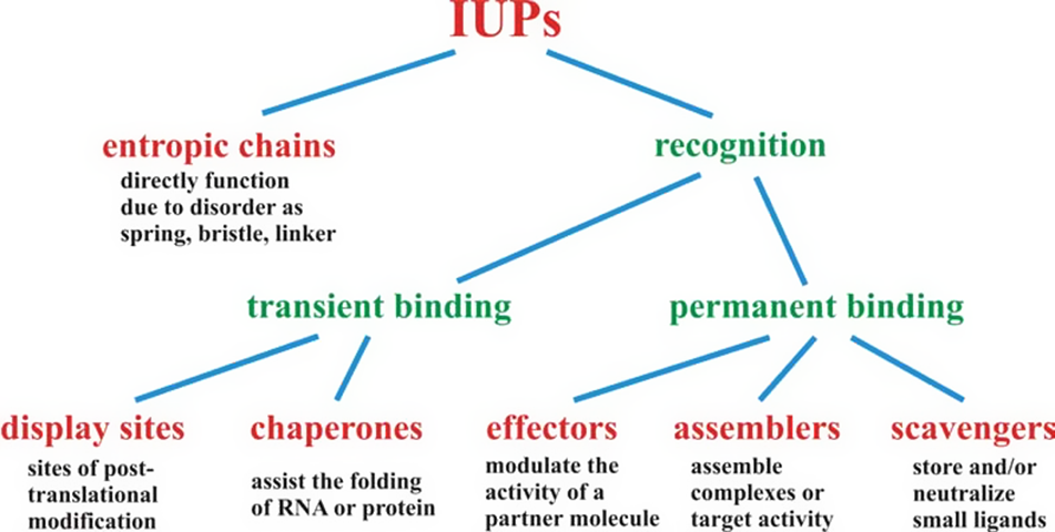
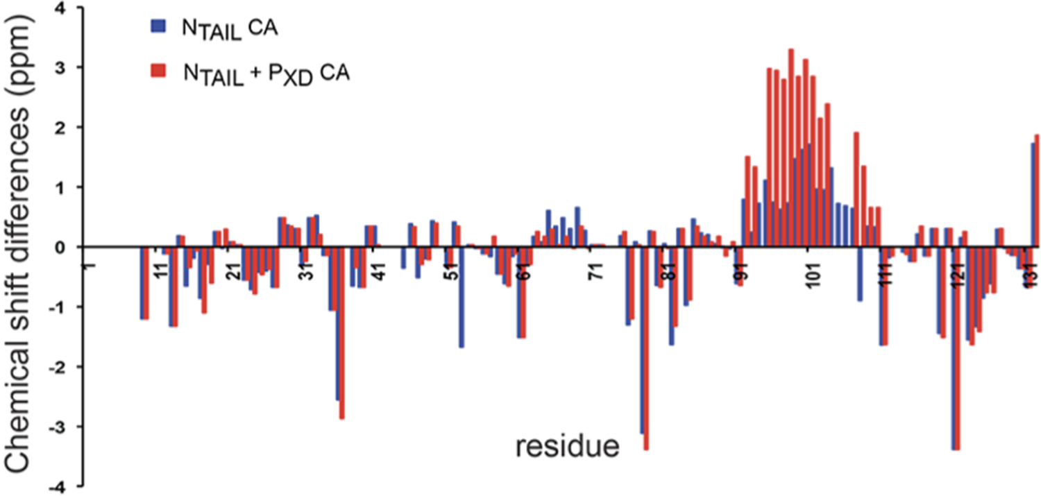


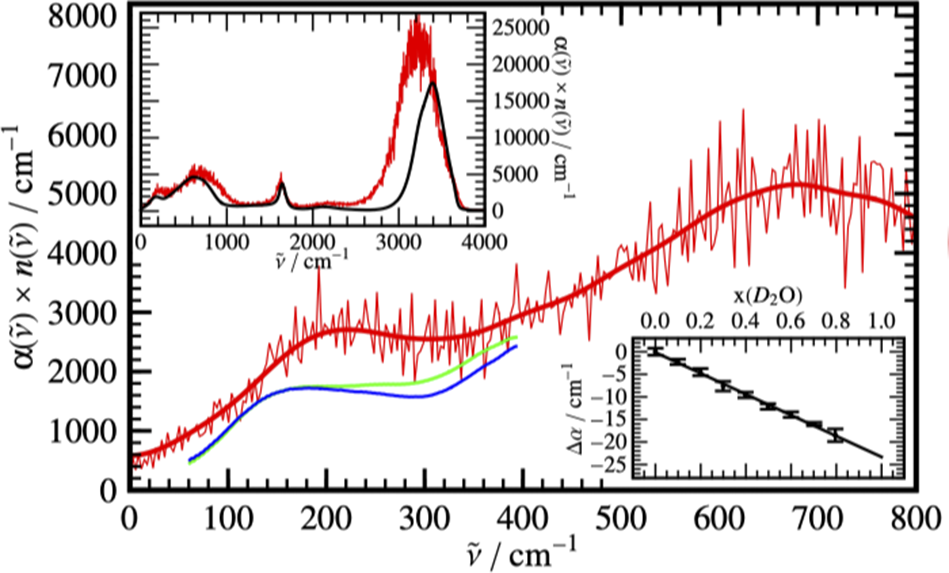


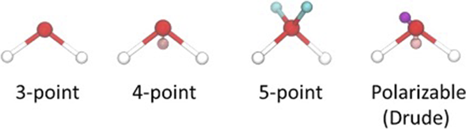


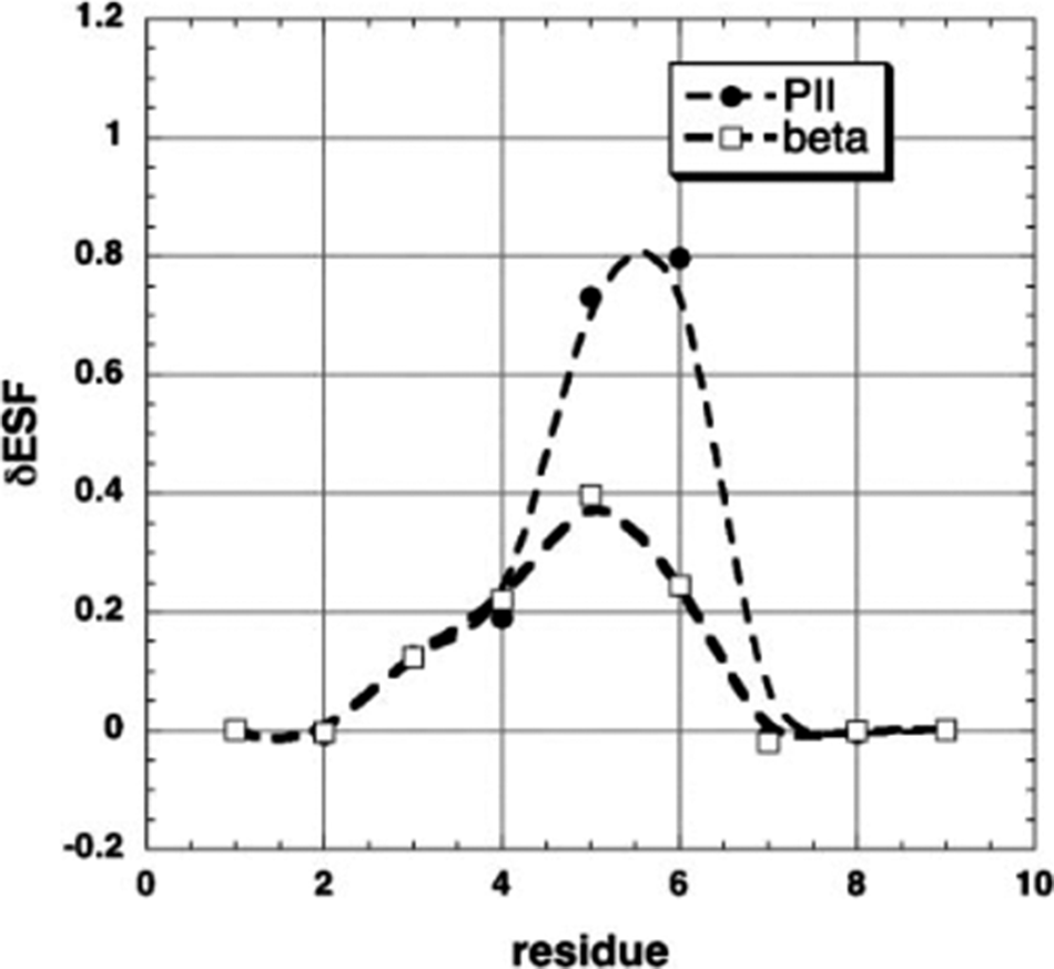
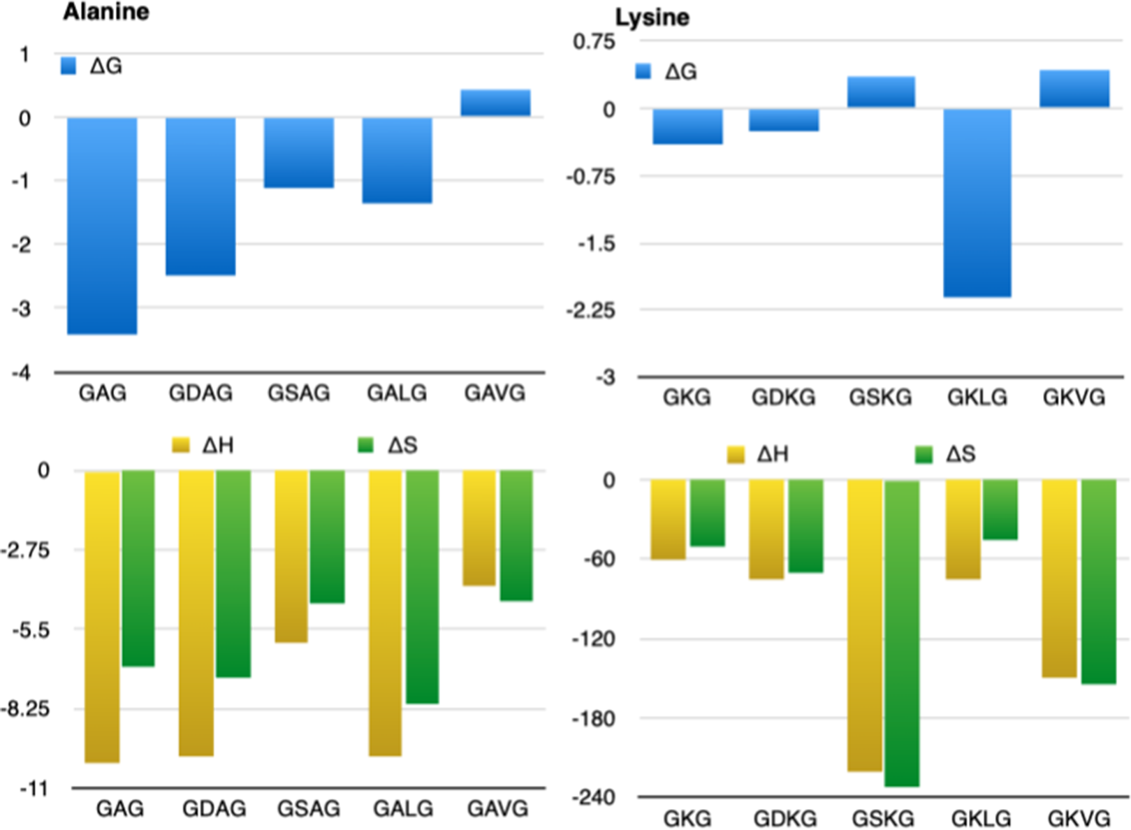

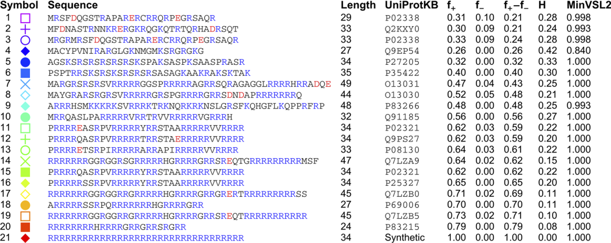
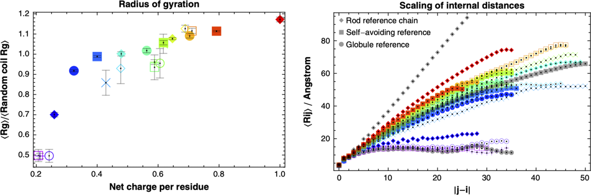

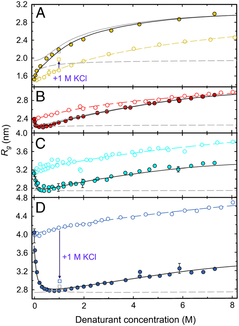


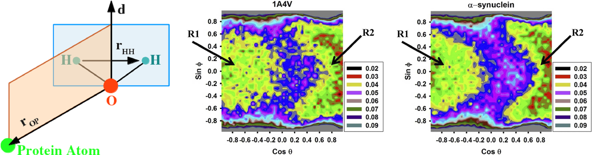


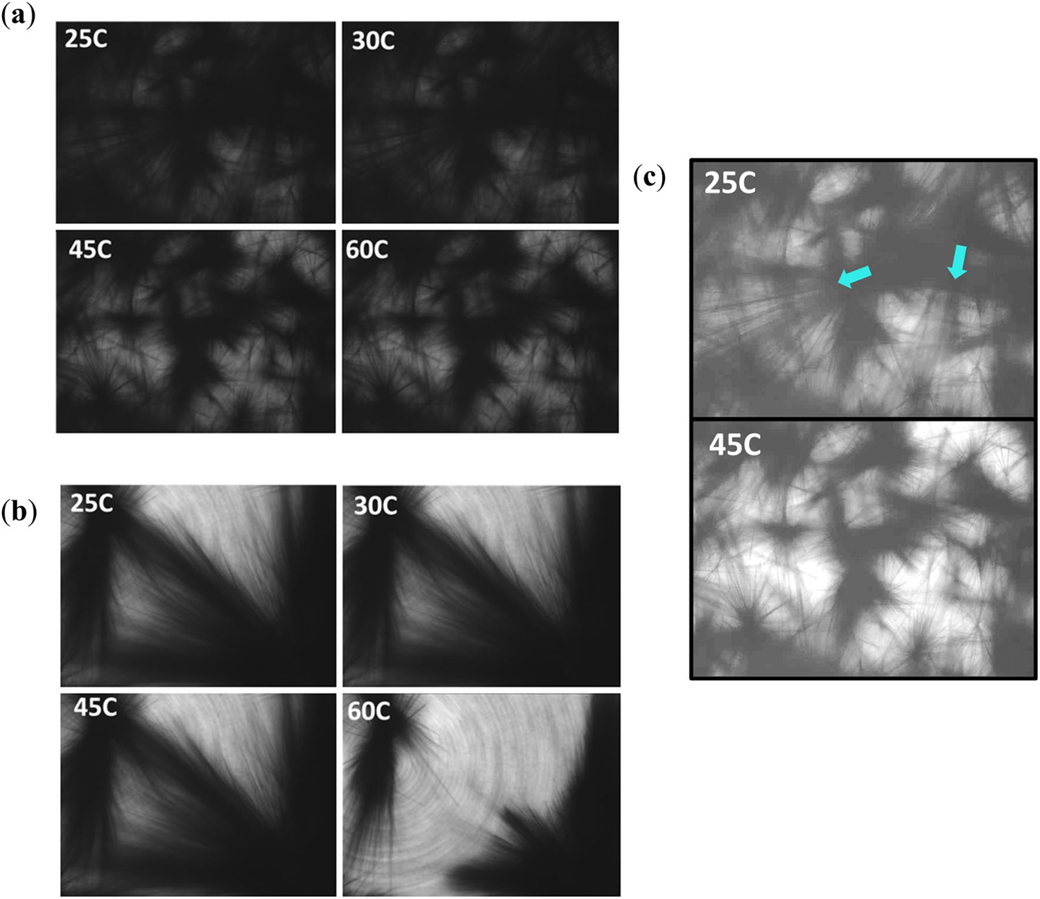
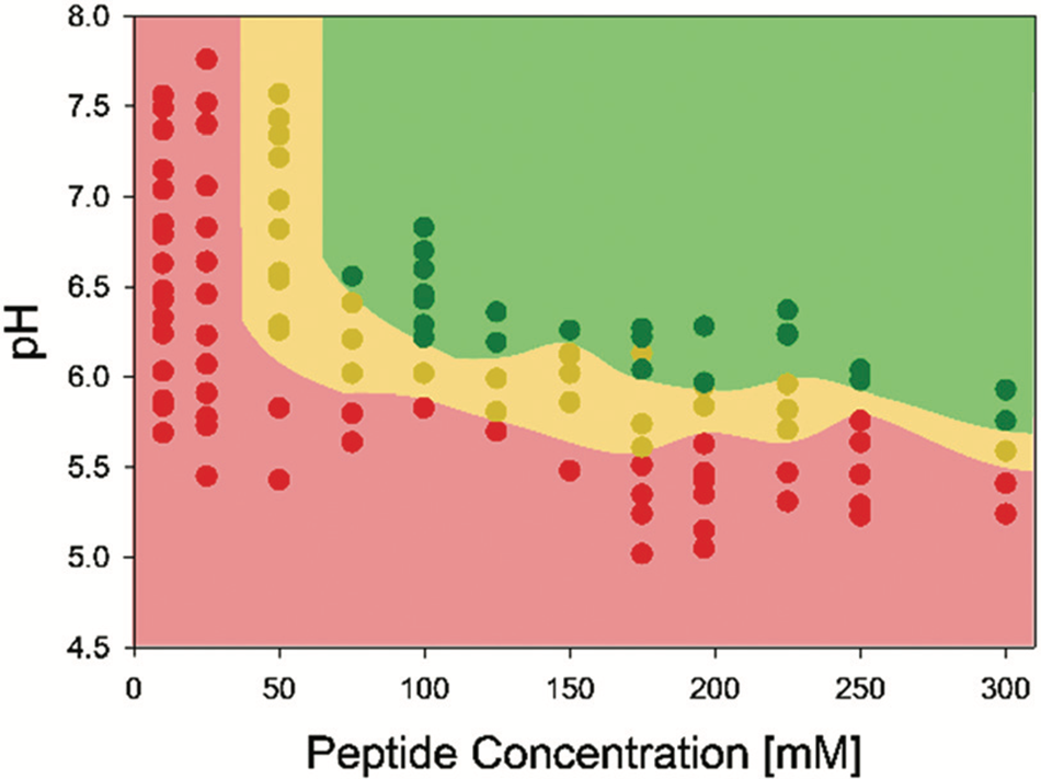
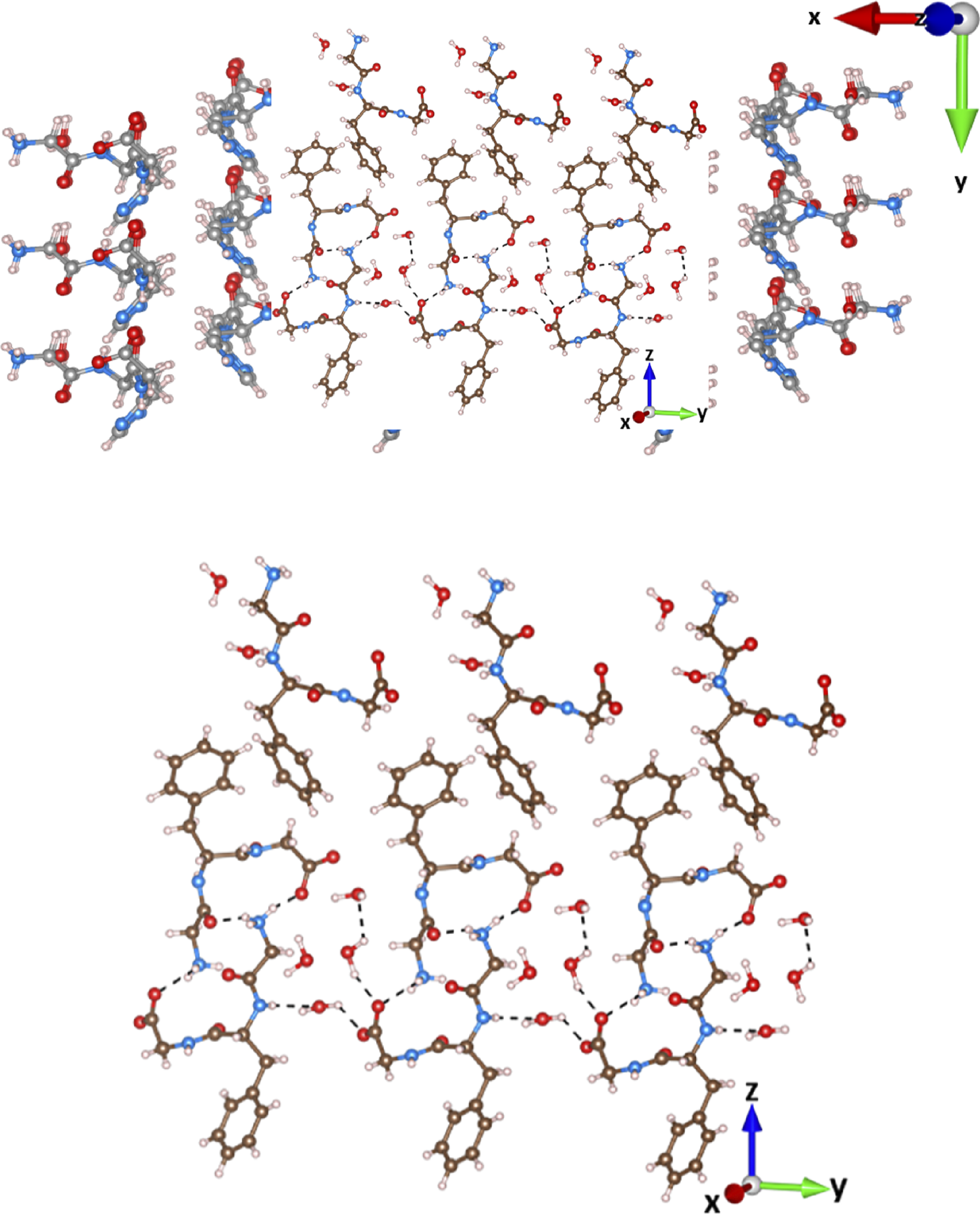

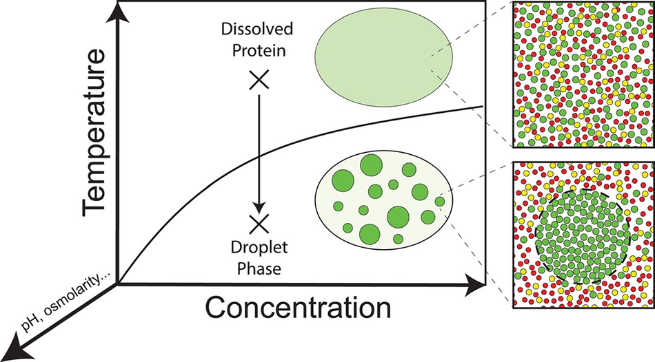
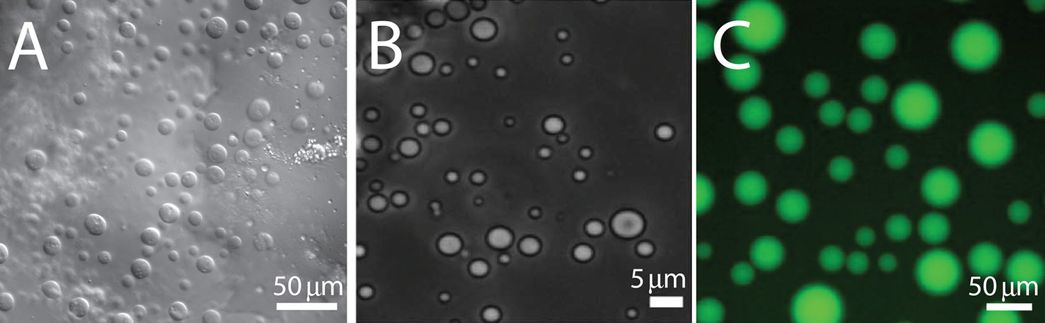

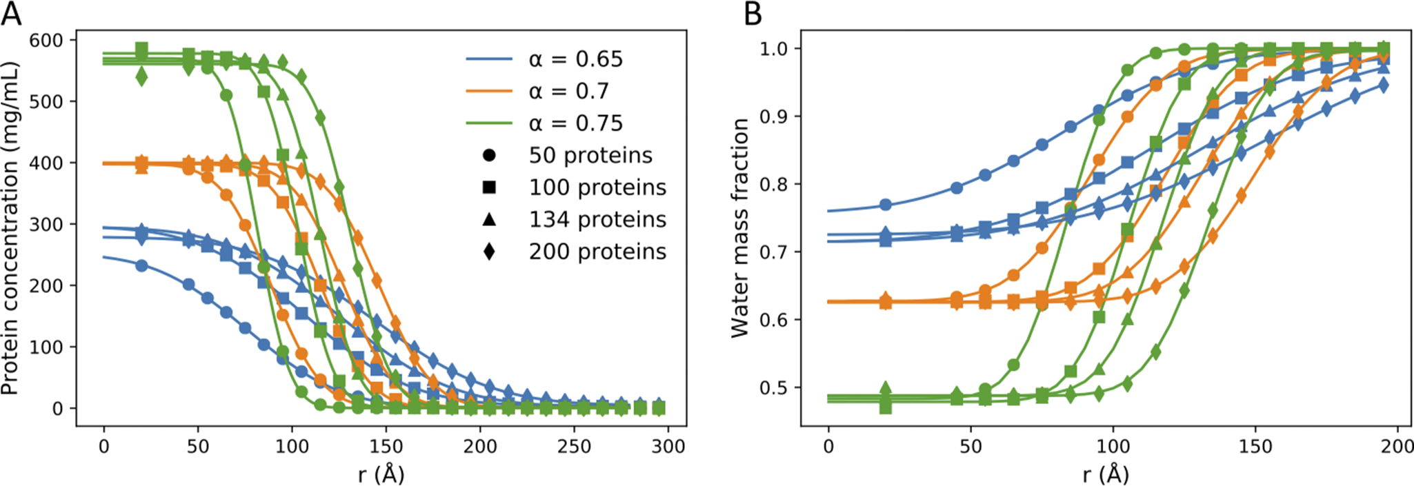

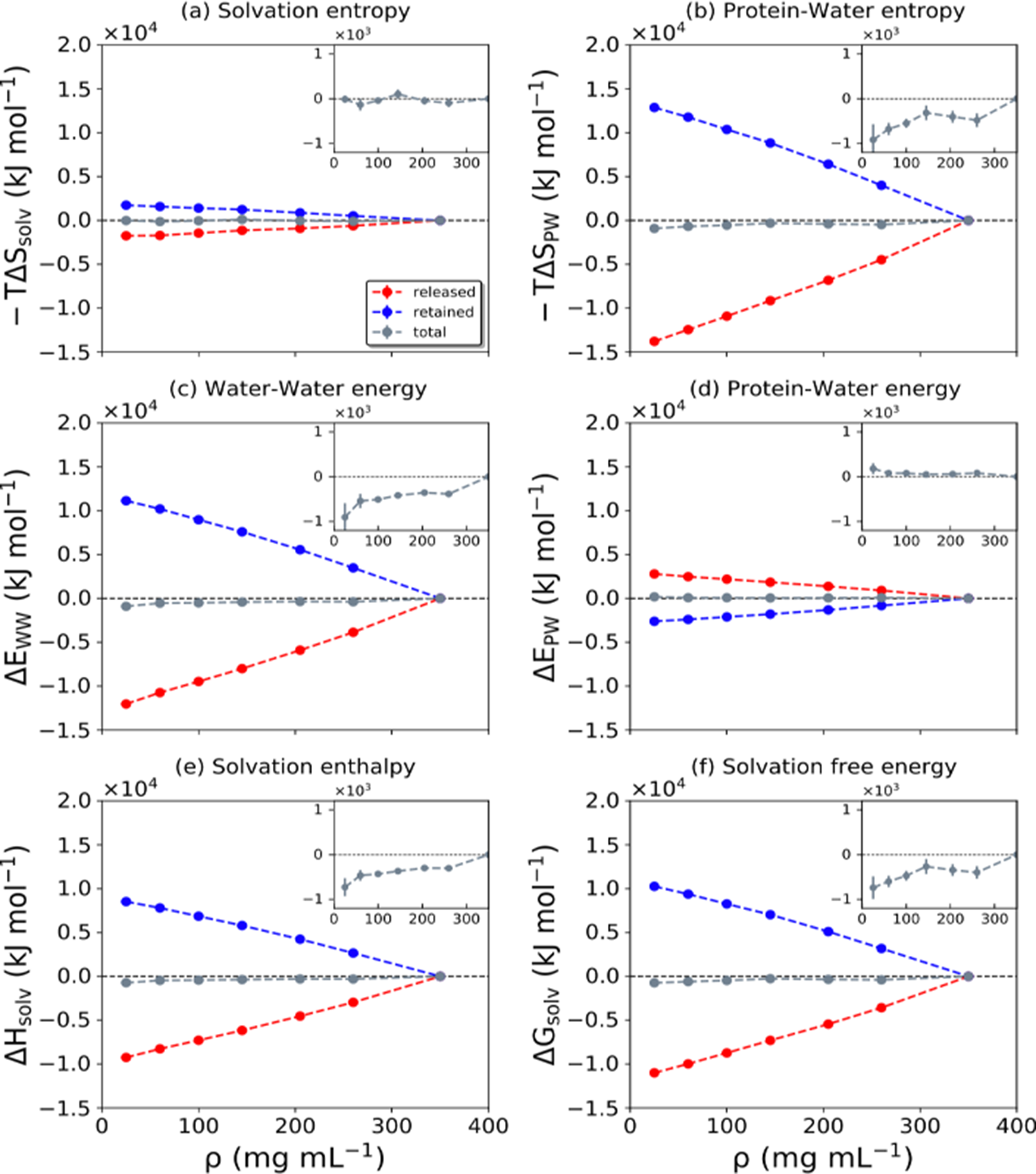

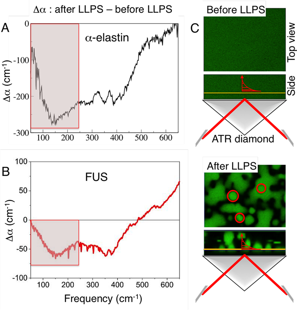
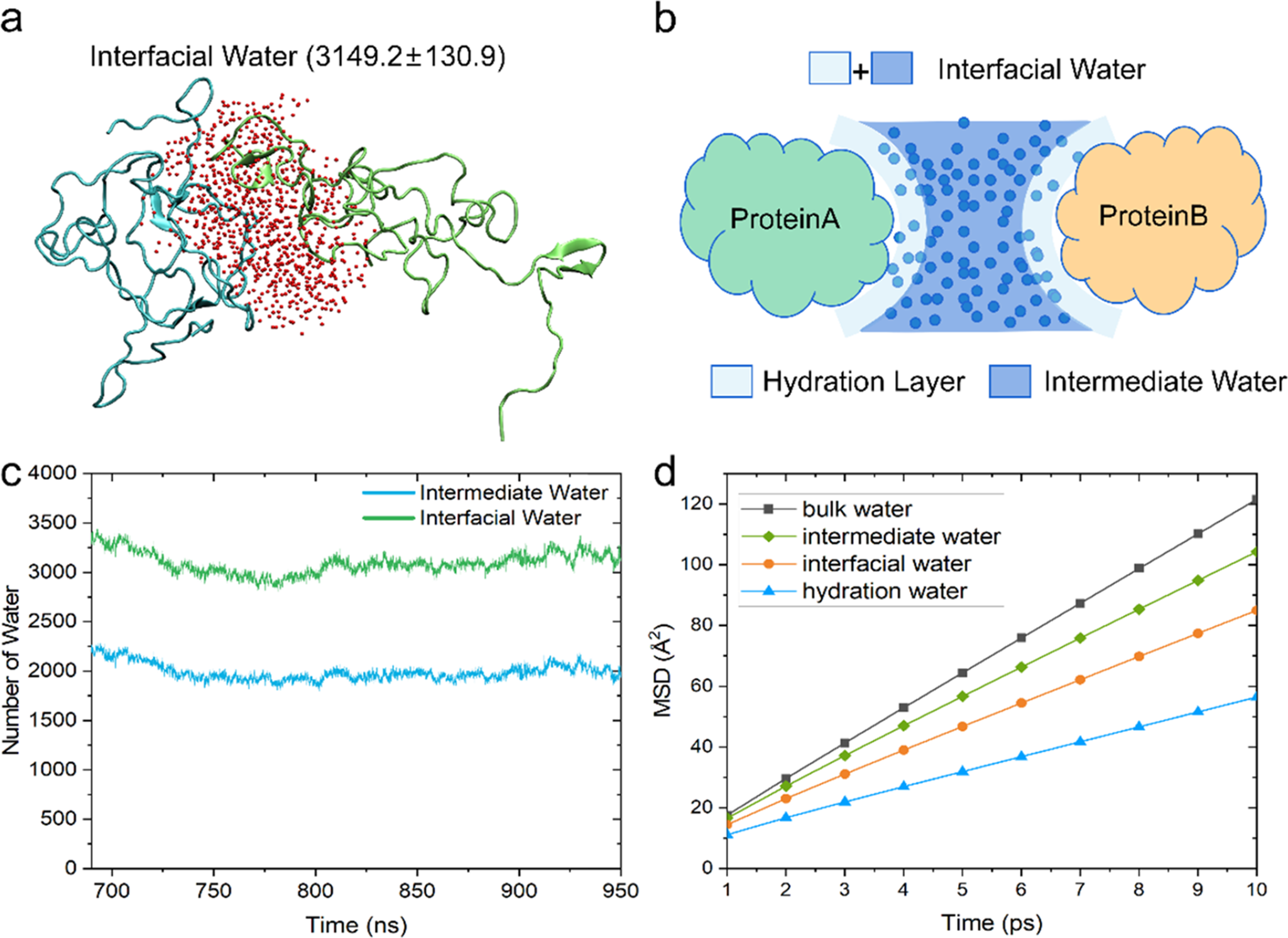

 Open access