

Introduction: force and displacement as controlled variables
Energy has been an essential concept in the vocabulary of biochemists and biophysicists as it permits a system of interest to be evaluated and analyzed under the powerful predictive value of thermodynamics. It furnishes the essential criterion to determine the spontaneity of a process, the affinity of binding partners, the likelihood of a spontaneous crossing of a thermal barrier, etc. Force, on the other hand, has been practically absent in the terminology of biological research in part because of the difficulty or impossibility of its implementation in traditional bulk or ensemble experiments. Force is indeed a mysterious quantity in physics. Its existence and interpretation have been a constant preoccupation of philosophers and scientists since antiquity. Often confused with energy, power, and momentum throughout history, its clear formulation and acceptance in mechanics had to await Newton's definition of his second law in his ‘Philosophia Naturalis Principia Mathematica’ published in 1687. Even after this crucial development, the interpretation of force as a physical entity has continued to be a source of much epistemological debate. See for example the excellent monograph on the subject by Max Jammer (Jammer, Reference Jammer1962).
Yet, force has been an implicit concept in physical chemistry all the way back to its foundational research period in the last quarter of the nineteenth century. In 1873, the Dutch scientist, Johannes D. van der Waals, proposed his theory of ‘Continuity of the Solid and Liquid States of Matter.’ In it, he states: ‘All properties of matter depend on the strength and the direction of the forces that molecules exert on each other.’ From today's perspective, this statement may seem self-evident and trivial, but van der Waals lived and worked at a time where one of the arguments utilized by the opponents of the molecular theory of matter was precisely the huge difference in the physical macroscopic properties of solids, liquids, and gases, which they argued could not be rationalized if matter was made up of discrete entities. Similarly, the idea that forces and torques develop in the course of chemical reactions is not new. In 1889, the Swedish scientist Svante Arrhenius (1859–1927) proposed that the rate of a chemical reaction is determined by how rapidly reacting molecules could reach and overcome a strained, high-energy, or activated state through collisions with other molecules along their reaction coordinate. The attainment of these strained, high-energy states requires the generation of torques and forces (stresses) acting on molecules. Despite their explanatory power, forces, torques, strains, and stresses, remained largely theoretical concepts as they were not under the control or the ability to measure by the experimentalist working with molecular ensembles.
The ability to apply and measure forces in a controlled manner at the single-molecule level has allowed scientists to revisit the theoretical concepts of force, torque, strain, and stress development in the course of chemical and biochemical reactions and has made the fundamental ideas of van der Waals and Arrhenius experimentally addressable. The development of single-molecule force spectroscopy has made it possible to think of many chemical and biochemical processes as being essentially mechanochemical phenomena and study them with the aid of externally applied forces and torques. Moreover, as a vectorial quantity, force has both direction and locality. Its application or generation in a reaction privileges the particular direction in which it acts and makes it possible to deliver energy (via the resulting displacement) both locally and selectively on one part of the molecule without necessarily affecting the rest. This locality gives researchers a great deal of flexibility in experimental design and implementation. Finally, force's conjugate variable, displacement, brings us back to more solid grounds as their product is the work done on or by the system and therefore a form of energy transfer, thus establishing the bridge between single-molecule force spectroscopic measurements and traditional bulk or ensemble experiments.
Beginnings
In 1981 I (C.B.) was a postdoctoral fellow in the laboratories of Ignacio Tinoco, Jr. (‘Nacho’) and Marcos Maestre in Berkeley, and John Hearst, a professor who had attended the Cold Spring Harbor Symposium on Quantitative Biology, gave a summary of the work presented that year to a group of students. He told us that one of the most surprising talks of the conference had been presented by a Japanese group that were able to observe molecules of DNA in solution under a fluorescence microscope with the molecules labeled with an intercalating fluorescent dye. I was profoundly impressed by the description of this work. It was a Eureka moment for me, and I remember thinking ‘Of course! It's just like watching constellations against a dark firmament! Why did I not think about that myself!’. I had to wait until the following year when the paper appeared published in the XLVII volume of the Symposia by M. Yanagida et al. (Yanagida et al., Reference Yanagida, Hiraoka and Katsura1983). I photocopied the paper the day before I left Berkeley to start my career as an independent researcher in the Chemistry Department of the University of New Mexico in Albuquerque. I remember promising myself to read the article as soon as I had time, and threw it into the trunk of my car, which I hauled behind a moving truck all the way to Albuquerque.
Once in New Mexico, I had to set aside my interest in this work and I concentrated to establish my research efforts on what had been my doctoral thesis and postdoctoral work, the characterization of the differential scattering between right- and left-circularly polarized light by chiral molecules. In 1984 I got a Searle Scholarship and for the first time I had enough discretionary funds to buy a fluorescence microscope. I knew that the paper was still in the trunk of my car, dirty and soiled with dust and oil, but there it was. With Tim Houseal, a postdoctoral fellow in the laboratory, we began to work on reproducing the results of the Japanese group but with the emphasis in externally manipulating the molecules. We watch with fascination how some molecules that were non-specifically attached to the glass slide by one end were stretched under the application of flow or of an electric field, and how they retracted themselves when the flow or the field were turned off. Soon after, with Marcos Maestre, we decided that we were going to use this approach to study how molecules of DNA moved during gel electrophoresis. We placed the molecules in a thin gel of agarose cast between a slide and a cover slip and look at them moving under the influence of an electric field in a fluorescence microscope. The experiments worked and the results were stunning. We could see how molecules moved and ‘reptated’ through the gel. We were recording the movies when one morning Tim brought to me the week's issue of Science and opened it in an article where an identical study had been performed by a group of scientists led by Steve Smith, at the University of Washington. I was shocked! I had been confident that nobody had thought about such experiments! It was hubris on my part. We were obliged to scramble our work. Within a week we had a paper finished and sent to Biochemistry, where it soon appeared as a rapid communication. The following February I presented a poster with our results at the Annual Meeting of the Biophysical Society and met Steven Smith, the person that had literally scooped us and who was also presenting his results. Our posters were far from each other, but we naturally sought each other and then spent the rest of the four days of the meeting talking about science and dreaming about the things that could be done next. In our study of the DNA electrophoresis the elastic behavior of the DNA molecule had become even more evident. I wanted to characterize that elastic behavior. Steve and I departed with me telling him that maybe one day we could work and collaborate doing some fun science together. One week later, back in Albuquerque, I received a letter from Steve where he told me that he had enjoyed greatly our meeting and that he wondered whether I really thought we could work together or if I had said that just out of politeness. I wrote back and invited him to join my laboratory and six months later we were working together to investigate the elastic properties of single DNA molecules.
DNA elasticity
The entropic elasticity regime
Steve and I discussed various schemes; first, we decided to use a molecule of lambda DNA to perform a ‘Physics 1’ experiment under an optical microscope. Treating the molecule as a spring, Steve, Laura Finzi – at the time a chemistry graduate student in my laboratory – an undergraduate student, and I began by attaching the DNA via one of its ends to the coverslip of a micro-chamber. We then stretched the molecule by hanging one, two, three, four, or five denser-than-water beads, from its free end. We were able to calculate the beads' weight under water and to determine the resulting molecular extension using the microscope focus. In this way we obtained the first force versus extension curve of a single polymer molecule. We used to joke that the experiment involved the largest instrument we had ever designed, since it required the gravitational force exerted by the whole planet on the beads. Despite its crude design, the experiment already revealed the highly non-linear character of the extensional elasticity of the DNA molecule (Bustamante et al., Reference Bustamante, Finzi, Sebring and Smith1991). Encouraged by this result, Steve, Laura, and myself decided to improve the experiment. In the new scheme, we used a dimer of lambda DNA to increase the signal-to-noise of our experiment. We bound the DNA molecule to the coverslip by one end as before, but attached a paramagnetic bead to the other end, so that we could apply increasing magnetic forces to the molecule by moving magnets closer to the side of the coverslip. To increase the range of forces applied to the molecule we combined the magnetic forces applied along the x-axis with flow forces applied along the y-axis. Inverting the direction of the magnetic and flow fields we were able to stretch the molecule along the four quadrants of the x-y plane. The extension of the molecule, measured from its point of attachment on the glass to the position of the magnetic bead, described an ellipse as the ratio of the flow over the magnetic forces increased and the molecule got more extended (see Fig. 1). For every position of the bead along this ellipse, the end-to-end extension of the molecule responded to a resultant force FR = FM sec(θ), where θ is the angle between the DNA molecule and the x-axis, and FM is the magnetic force applied. For every bead position (angle θ) the resultant force acting on the molecule could be determined simply by measuring the magnitude of the magnetic component and the angle θ.
(a) A microchamber made from slide and cover slip. Magnets (1 cm diameter) were moved to repeatable positions as close as 9 mm from the objective's center. Buffer flow was maintained by a constant pressure system. A computer cursor superimposed on the microscope image was used to record the equilibrium bead positions, time-averaged over their Brownian motion. The magnetic bead was tethered by a DNA molecule. (b) Ellipse of bead positions (●) obtained from various combinations of flow and magnetic forces (determined by Stokes' law). The strongest magnet force is FM. The flow force is FMtan(θ), and the total force stretching the DNA along θ is FMsec(θ). Low-force positions (○) at zero flow and weak magnetic forces. (c) The extension of DNA is the shortest path from its point of attachment on the bead to that on the glass. Each bead is internally anisotropic, giving it a permanent magnetic dipole μ that nearly aligns with the external magnetic field B. The bead attachment point is constrained to some arbitrary latitude line, with the bead free to rotate about μ and minimize the DNA extension. This constraint is removed in the high-flow zero-magnet cases. By selecting a ‘best fit’ latitude for each bead, the force versus extension data on the ellipse converge to one continuous curve, characteristic of the polymer. Reprinted with permission from Smith et al. (Reference Smith, Finzi and Bustamante1992).

To determine the magnetic force, we detached the bead from the molecule using a laser beam and measured the velocity attained by the bead for the same magnet position. According to Stokes' law, the magnetic force is simply FM = 6πηrv, where v is the measured bead velocity, η is the viscosity of the water, and r is the radius of the bead. The resulting force versus extension curves spanning between 40 femto Newtons (fN) and 10 pico Newtons (pN) can be seen in Fig. 2. The non-linear nature of the extensional response of a polymer is clearly evident. Our paper appeared in 1992 (Smith et al., Reference Smith, Finzi and Bustamante1992).
Force versus extension data for four different λ-DNA dimer molecules (●, □, +, and ○) in 5 mM Na2HPO4 buffer (10 mM Na+, pH 8.3). Inset: expanded vertical scale (0–0.5 pN). Continuous curves are FJC models assuming a DNA contour length L = 32.7 μm and Kuhn segment b = 500 Å (top), 1000 Å (middle), and 2000 Å (lower). L = 32.7 μm was chosen to agree with the accepted value of 3.37 Å rise per base pair, not to fit the data. Reprinted with permission from Smith et al. (Reference Smith, Finzi and Bustamante1992).
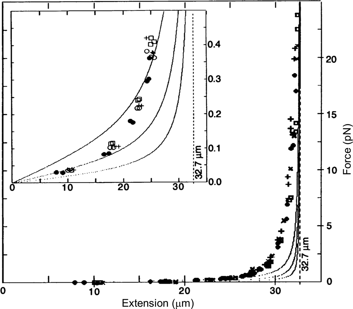
Under the forces applied to the molecule its end-to-end distance never reaches its theoretical contour length (indicated by the vertical dashed line in Fig. 2), because in this regime of forces these only align the segments of the molecule against the disorder exerted by the thermal bath. As we mechanically extend the molecule by an amount Δx, we greatly reduce the number of its accessible configurations reducing, correspondingly, its entropy. The reversible work done in extending the molecule (the area under the force-versus-extension curves in Fig. 2) is then simply proportional to the entropy change, ΔS, of the molecule, w = –FΔx = TΔS, where T the absolute temperature. This behavior corresponds to the so-called entropic elasticity of a polymer. In the 1992 article we tried to fit the data to the freely jointed chain (FJC) model of polymer elasticity. This model assumes that the molecule is made up of straight segments, known as Kuhn segments (after Hans Kuhn who introduced the concept in 1930s) that are completely free to adopt any orientation in space. In this model the elastic response of the polymer is parametrized by the size (length) of its Kuhn segments. The stiffer the molecule the longer its Kuhn segments. Our data, obtained using the combination of flow and magnetic forces, were precise enough to show that the FJC model did not correctly describe the elastic response of a DNA molecule. The idealization of a molecule made up of identical segments whose lengths are fixed and force independent greatly neglects many of configurations accessible to the molecule at any given force. In reality, any segment of a molecule placed in a thermal bath will bend smoothly and slightly in response to thermal fluctuations.
In 1994, Eric Siggia and John Marko approached me to test the idea that the worm-like chain (WLC) model could provide a better fit for the elastic response of dsDNA; this model describes the molecules as behaving locally as Hookian springs, deviating slightly and smoothly from their straight configuration due to thermal fluctuations. Introduced initially by Kratky and Porod in 1949 (Kratky and Porod, Reference Kratky and Porod1949) and later elaborated by Landau and Lifshitz (Landau and Lifshitz, Reference Landau and Lifshitz1980), the WLC model describes the elasticity of a molecule at equilibrium in a thermal bath in terms of its persistence length, P. The persistence length can intuitively be described as the distance along the molecule through which the memory of its initial orientation persists. Stiffer molecules have larger persistence lengths. Mathematically, the model posits that the average autocorrelation between unit tangents to the molecule at two different points decays exponentially with the separation s between the two points at a rate proportional to its persistence length: $ \langle\hat{t}( 0 ) \cdot {\rm \;}\hat{t}( s )\rangle = e^{-( s/P) }$ . The FJC and the WLC models can be used to predict the statistical properties of the molecules, such as its mean square end-to-end distance or its radius of gyration. The results of the mean square end-to-end distance, <(Δx)2>, are: <(Δx)2>FJC = Lb, where b is the length of the Kuhn segment and L is the contour length of the molecule, and <(Δx)2>WLC = 2PL. The two results can be reconciled by identifying a Kuhn segment as twice the persistence length of the molecule. While the fact that both models make similar predictions is satisfactory, it is also clear that in the absence of an applied force, when the molecules are only subjected to thermal fluctuations, the average statistical parameters derived from ensemble experiments cannot be used to determine which of these two models more appropriately describes the elastic behavior of the molecule.
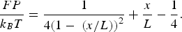
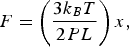
In their derivation of the effect of an applied external force F on the end-to-end distance x of a WLC of contour length L attached to a wall by one end, Eric Siggia and John Marko were able to describe two extreme regimes of the molecule: the low-force or linear regime, where the extension of the molecule is proportional to the force, with the molecule behaving as a linear spring that follows Hooke's law: ‘uc tensio sic vis’ or ‘as the extension so goes the force’; and the high-force regime in which the extension grows proportional to the inverse of the square-root of the force. It is possible to combine these two regimes into an extrapolation formula (Bustamante et al., Reference Bustamante, Marko, Siggia and Smith1994; Marko and Siggia, Reference Marko and Siggia1995):
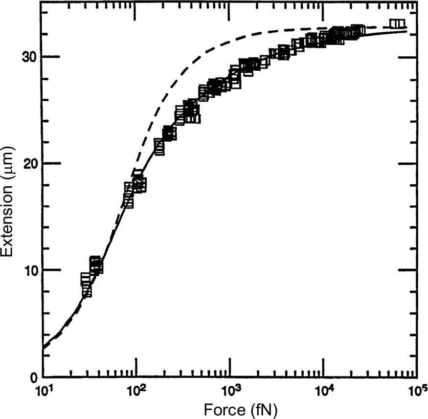
A comparison between the FJC and the WLC models can be seen in Fig. 3 wherein it is clear that the latter describes much better the elastic response of the DNA molecule. The application of a stretching force to the molecule thus made possible to discriminate between the predictions of two models of polymer elasticity. For DNA dissolved in 10 mM NaCl, the best fit was obtained for a persistence length of 53 nm (Bustamante et al., Reference Bustamante, Marko, Siggia and Smith1994).
Squares are experimental force versus extension (F-x) data for 97 kb λ-DNA dimers from Smith et al. (Reference Smith, Finzi and Bustamante1992). Solid line is a fit of the entropic force required to extend a worm-like polymer. The fit parameters are the DNA contour length (L = 32.80 ± 0.10 μm) and the persistence length (P = 53.4 ± 2.3 nm). Shown for comparison (dashed curve) is the freely jointed chain model (Smith et al., Reference Smith, Finzi and Bustamante1992) with L = 32.7 μm and a Kuhn segment length b = 100 nm chosen to fit the small-x data. Reprinted with permission from Bustamante et al. (Reference Bustamante, Marko, Siggia and Smith1994).
When x/L << 1, we can expand Eq. (1) and obtain Hooke's law:
with the spring constant given by the term in parenthesis. Note that the stiffer the molecule, i.e., the larger its persistence length, the smaller its spring constant, and the easier it is to extend it. Also, the longer the molecule, the easier it is to align it with the force.
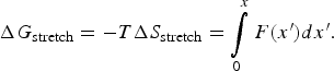
Tethering a dsDNA molecule to the beads by the 3′- and 5′-ends of the same strand, it was possible to melt-off the unlabeled strand by subjecting the molecule to successive cycles of extension and relaxation, either in water or in 20% formaldehyde. These experiments allowed us to obtain the force-extension curves of ssDNA (Fig. 4). ssDNA is more flexible and more contractile than dsDNA; therefore, at the beginning of the extension cycle, it takes more force to extend it than dsDNA. However, dsDNA has a shorter contour length than ssDNA, and the force needed to continue to extend the duplex eventually increases rapidly. The two curves cross at ~7 pN. Above this force, dsDNA is markedly harder to extend than ssDNA (see section ‘DNA polymerase’). We found that it was possible to fit the force-extension curve of ssDNA using an extensible freely-jointed chain model (Smith et al., Reference Smith, Cui and Bustamante1996), which yielded a persistence length of 0.75 nm. This analysis shows that the braided structure of the DNA duplex is responsible for being nearly 70 times stiffer than its component strands.
A λ-phage ssDNA molecule was stretched in 150 mM NaCl, 10 mM Tris-HCl, 1 mM EDTA, pH 8.0 (green triangles). The dashed line represents the elasticity of a freely jointed chain (FJC). The continuous line represents an extensible FJC with stretch modulus. Figure adapted and reprinted with permission from Smith et al. (Reference Smith, Cui and Bustamante1996).
This large difference in elastic response between these two forms of the molecule furnishes the basis of assays designed to monitor the activity of DNA polymerases and other non-processive enzymes (see section ‘DNA polymerase’). Ritort and collaborators have performed a systematic analysis of the elasticity of single-stranded DNA over two-orders of magnitude of monovalent and divalent salts (Bosco et al., Reference Bosco, Camunas-Soler and Ritort2014). These authors found an intrinsic persistence length of 0.7 nm with the electrostatic contribution to the persistence length varying as the inverse of the cation concentration.
As mentioned before, in the force regime in which Eq. (1) applies, the work done on the molecule to stretch it only changes its entropy. Thus we can write (Tinoco and Bustamante, Reference Tinoco and Bustamante2002):
Using Eq. (1) and integrating we obtain:

As expressed in Eqs. (1) and (4), the force, the free energy, and the entropy are all inversely proportional to the persistence length of the molecule. From Eq. (1) we obtain that the force needed to stretch a double-stranded DNA molecule at 298 K to 75% of its contour length (x/L = 0.75), assuming a persistence length of 53 nm, is 0.37 pN. A similar fractional extension of a single-stranded DNA, assuming a persistence length of 1 nm, requires a force of 19.5 pN. Similarly, the stretching free energy for a double-stranded DNA molecule of 2940 base pairs (bp) is 2091 kJ mol–1, and for a single-stranded DNA with 1700 nucleotides (nt) is 41.8 kJ mol–1.
The intrinsic elasticity regime
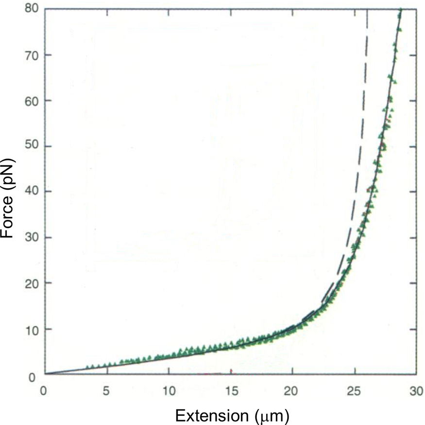
In 1996, Steve Smith, myself (C.B.), and a graduate student, Yujia Cui began to investigate the elasticity of the DNA beyond the entropic regime. Using an optical tweezers instrument that employed the principle of conservation of linear momentum (Smith et al., Reference Smith, Cui and Bustamante2003), we were able to subject the molecule to forces greater than 10 pN. At this force the molecule is more than 96% extended and the force applied to its ends begins to distort the very fabric that maintains the molecule's structure, the stacking interactions between its base pairs. As we continue to increase the force on the molecule, we find that it reaches and eventually crosses its theoretical Watson–Crick contour length at about 40 pN. The molecule continues to extend beyond this length displaying a stretch modulus of 1100 ± 200 pN (Smith et al., Reference Smith, Cui and Bustamante1996). For applications involving forces above 30 pN, an empirical correction that takes into account this stretch modulus can be employed (Wang et al., Reference Wang, Yin, Landick, Gelles and Block1997b; Bustamante et al., Reference Bustamante, Chemla, Liu and Wang2021). Then, depending on the ionic strength conditions, as the force increases above 60 pN, the molecule undergoes a sudden, cooperative, and reversible transition reaching an extension of ~70% over its contour length. At the time we suggested that this ‘overstretched’ form of the molecule should correspond to a distinct structure that we called S-DNA. We communicated this observation of the overstretching transitions simultaneously with a group in France (Cluzel et al., Reference Cluzel, Lebrun, Heller, Lavery, Viovy, Chatenay and Caron1996; Smith et al., Reference Smith, Cui and Bustamante1996). Several groups challenged the assertion that under high tensions the molecule adopts a distinct structural form. In their view, S-DNA was not a distinct structural form of the molecule but denatured DNA (Rouzina and Bloomfield, Reference Rouzina and Bloomfield2001a, Reference Rouzina and Bloomfield2001b; Williams et al., Reference Williams, Wenner, Rouzina and Bloomfield2001a, Reference Williams, Wenner, Rouzina and Bloomfield2001b; Shokri et al., Reference Shokri, McCauley, Rouzina and Williams2008; van Mameren et al., Reference Van Mameren, Gross, Farge, Hooijman, Modesti, Falkenberg, Wuite and Peterman2009). The controversy persisted for a few years until it was eventually settled when all groups involved agreed that above 65 pN, the molecule adopts a structure, different from its denatured form (Bosaeus et al., Reference Bosaeus, El-Sagheer, Brown, Smith, Akerman, Bustamante and Norden2012; King et al., Reference King, Gross, Bockelmann, Modesti, Wuite and Peterman2013; Zhang et al., Reference Zhang, Chen, Le, Rouzina, Doyle and Yan2013). In collaboration with the group of Bengt Nordén at Chalmers University, we applied these high forces to very short molecules of DNA that could be prevented from denaturation by cross-linking of both of their ends (Bosaeus et al., Reference Bosaeus, El-Sagheer, Brown, Smith, Akerman, Bustamante and Norden2012). With molecules with a high GC content (60%) it was possible to clearly distinguish the overstretching transition from melting. In these cases, the molecule displayed an end-to-end extension of 50% above its contour length (Fig. 5). Accordingly, the 70% increased seen in the original work (Bustamante et al., Reference Bustamante, Marko, Siggia and Smith1994; Marko and Siggia, Reference Marko and Siggia1995) represent the combined contribution of overstretching and some frying from pre-existing nicks in the molecule. Significantly, a 50% increase in extension is precisely what results from the binding of RecA or Rad51 to DNA (Chen et al., Reference Chen, Yang and Pavletich2008; Reymer et al., Reference Reymer, Frykholm, Morimatsu, Takahashi and Norden2009). The existence of a defined overstretched state accessible directly by mechanical means suggests that evolution may have simply taken advantage of this inherent property of the molecule for the process of homologous recombination. A future task will be to establish the structure of the overstretched or S-form DNA.
Stretching of λ-phage dsDNA in 150 mM NaCl, 10 mM Tris-HCl, 1 mM EDTA, pH 8.0 (black diamond). The ‘inextensible wormlike chain’ curve is from Bustamante et al. (Reference Bustamante, Marko, Siggia and Smith1994), for a persistence length of 53 nm and a contour length of 16.4 μm. Reprinted with permission from Smith et al. (Reference Smith, Cui and Bustamante1996).
Many articles using single-molecule force spectroscopy of ss- and dsDNA have appeared since the original work described here. The interest has extended beyond the biophysical community to the polymer physics community. The reason, in part, is that unlike non-biological polymers, DNA molecules can be prepared as mono-disperse samples making it possible to investigate many aspects of polymer elasticity and to test and formulate alternative theoretical models. For a recent review see Camunas-Soler et al. (Reference Camunas-Soler, Ribezzi-Crivellari and Ritort2016).
The torsional elasticity of dsDNA
Having investigated the non-linear elastic behavior of DNA we turned to characterize its torsional elasticity. The motivation from these studies arose in part from experiments performed in the laboratory of David Bensimon and Vincent Croquette at the Ecóle Normal Superieur in Paris (Strick et al., Reference Strick, Allemand, Bensimon, Bensimon and Croquette1996). These authors used a rotating magnet to twist and supercoil both positively and negatively (i.e., overwind and unwind) single molecules of DNA, which were torsionally constrained through attachments at one end to a glass surface and at the other to a magnetic bead while subjected to force. The magnitude of the force applied to the molecule was determined from its effect on the observed Brownian fluctuations of the bead in the image plane. These experiments revealed sharp transitions, which involve a change in extension for both underwound and overwound molecules and correspond to the formation of plectonemes.
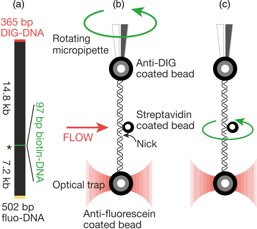
That work was our motivation to measure the torsional rigidity of the molecule, a parameter that ultimately determines its behavior under torsion and its partition between writhe and twist. Moreover, many DNA-binding proteins are known to unwind the double helix, including helicases and regular binding proteins such as TATA-box binding protein and enzymes such as homing endonuclease I-ppoI (Becker and Everaers, Reference Becker and Everaers2009); the energy involved in the process depends on the torsional rigidity of the molecule. Thus, because of its importance, several groups had previously used various ensemble methods to measure this quantity for dsDNA. Its value showed great dispersion among the different ensemble methods used to determine it. For example, fluorescence polarization anisotropy experiments yielded a value of 200 pN⋅nm2 (Selvin et al., Reference Selvin, Cook, Pon, Bauer, Klein and Hearst1992). Using the distribution of topoisomers in gel electrophoresis a value of 300–400 pN⋅nm2 was obtained (Horowitz and Wang, Reference Horowitz and Wang1984; Heath et al., Reference Heath, Clendenning, Fujimoto and Schurr1996), and circularization kinetics methods gave a value as high as 480 pN⋅nm2 (Shore and Baldwin, Reference Shore and Baldwin1983). Finally, the average value derived from topoisomer distribution of small DNA circles gives a value of 300 ± 100 pN⋅nm2 (Crothers et al., Reference Crothers, Drak, Kahn and Levene1992). The large dispersion among the different measurements likely reflects the fact that in ensemble methods the torsional stress introduced in the molecule necessarily partitions between writhe and twist. This partitioning will vary from method to method and, in general, will tend to reduce the apparent torsional rigidity to twist the molecule. Two graduate students in Molecular and Cell Biology, Zev Bryant and Michael Stone became interested in measuring this quantity directly on a single molecule. The experimental method is shown in Fig. 6. They attached a single DNA molecule between two beads in a torsionally constrained manner via multiple antigen-antibody linkages. One of the beads was held through suction by a micropipette and the other was held in an optical trap. The molecule was subjected to a tension of 15 pN to prevent it from writhing when twisted. A single nick in one of the strands was engineered one-third from one of the ends of the molecule so that rotation around a single bond in the backbone of the molecule could take place. They attached a third small bead (the ‘rotor’) to the side of the DNA molecule via biotin-streptavidin linkage just above the nick. The experiment consisted in introducing torsional strength in the molecule by rotating the micropipette. At the beginning of the experiment, flow was introduced in the chamber, so that the rotor bead could be held fixed on one side of the molecule to prevent it from turning about the single strand in front of the nick while the pipette was rotated via a computer-controlled motor to introduce torsional stress in the molecule. Once the desired number of turns in the molecule had been introduced, stopping the flow would allow the small bead to rotate as the twisted molecule unwound.
(a) The molecular construct contains three distinct attachment sites and a site-specific nick (*), which acts as a swivel. (b) Each molecule was stretched between two antibody-coated beads using a dual-beam optical trap (Smith et al., Reference Smith, Cui and Bustamante2003). A rotor bead was then attached to the central biotinylated patch. The rotor was held fixed by applying a fluid flow, and the micropipette was twisted to build up torsional strain in the upper segment of the molecule. (c) Once the flow was turned off, the central bead rotated to relieve the torsional strain. Reprinted with permission from Bryant et al. (Reference Bryant, Stone, Gore, Smith, Cozzarelli and Bustamante2003).
The torque τ stored in a cylinder of length L that has been twisted by an angle ϕ is τ = C(ϕ/L), where C is the coefficient of torsional rigidity. This expression is valid for small angles or for linear torsional springs. Moreover, as the molecule unwinds, the torque stored for any given twist angle ϕ(t) is given by τ(t) = C(ϕ(t)/L) = ξ rotω(τ). In other words, as the molecule unwinds, the instantaneous value of the torque stored in the molecule can be determined from the angular velocity of the rotor bead, ω(τ), and the drag coefficient of a bead that rotates eccentrically around the molecule, ξ rot. For a bead of radius r, ξ rot = 14πηr 3.
Figure 7 shows that the torque stored in the molecule increases linearly with twist angle ϕ(t). Interestingly, despite the chiral nature of the molecule, the slope of the torque stored with the twist angle is constant and the same for over- and under-twisting DNA. The slope corresponded to a value of C = 440 ± 30 pN⋅nm2 (Bryant et al., Reference Bryant, Stone, Gore, Smith, Cozzarelli and Bustamante2003). Therefore, although DNA is a highly non-linear extensional spring, it behaves linearly as a torsional spring. These experiments yielded a value of the coefficient of torsional rigidity of DNA 50% larger than the average of 300 pNnm2 accepted at the time. We performed an independent estimation of this parameter using the same geometry as before but at zero twist and recording the angular fluctuations of the bead. Using the equipartition theorem, according to which, the energy associated with the mean quadratic angular fluctuation of the rotor bead should be equal to one half of kBT. Mathematically, (1/2)(C/L)<Δϕ 2 >= (1/2)k BT. These experiments gave a value of C = 460 ± 30 pN⋅nm2, confirming our previous result. Something really funny happened while Zev and Mike were doing the experiments. They had had a rough time getting all the many parts of the experiment to work simultaneously. Finally, one day, it was 3 am when everything seemed to be working. Now they had to introduce a number of turns to the micropipette (of the order of 500) and were doing so manually. So, one of them would turn a small handle and begin to count one, two, three, etc, by the time they were in the hundreds any distraction made them loose their count; they were decided to do the experiment well and so they had to begin all over again. In the middle of this frustration, Jan Liphardt, then a postdoctoral fellow in the lab, told them that what they needed was a motor that could be hooked to the computer. Zev and Mike agreed but, where to find such a motor at 3:30 am! Much to their surprise Jan told them that he had a motor of his Lego set. Apparently, he went everywhere with it and it was in his apartment. He lived only two blocks from campus, so he went and brought it back for them to interface it to the instrument. It worked like a charm! Zev and Mike were still in the lab when I arrived later that morning, and with a big smile they told me that they had a working experiment. I approach the optical tweezers instrument and I saw all these color Lego blocks, red, blue, green, yellow, white in the middle of the optics and holding the motor that was twisting the pipette. When they explained to me what had happened, we all agreed that we would complete all the data with that motor. When the paper was published in Nature a few months later (Bryant et al., Reference Bryant, Stone, Gore, Smith, Cozzarelli and Bustamante2003), we appropriately provided all the specifications of this efficient little motor that had done so well the tedious job of turning the pipette.
Twist elasticity of DNA. τC, critical torque. Negative torques: average of 39 runs at 15 pN. Positive torques: 37 runs at 45 pN and 27 runs at 15 pN gave very similar traces and were averaged together. Green lines, constant-torque structural transitions. Blue, linear fit to the data points falling within ±8 pN⋅nm. Anharmonic models (C(Δθ) = a − bΔθ/N, where N = 14 795 bp) give superior fits to the data over the full range of B-DNA stability. Red, two-parameter anharmonic fit (b/a = 4.5); dashed purple, anharmonic fit constraining b/a = 8.16 to agree with FPA data (Selvin et al., Reference Selvin, Cook, Pon, Bauer, Klein and Hearst1992). Blue and red fits give C(0) = 4.1 × 10² pN⋅nm2; purple fit gives C(0) = 4.3 × 10² pN⋅nm2. Figure adapted and reprinted with permission from Bryant et al. (Reference Bryant, Stone, Gore, Smith, Cozzarelli and Bustamante2003).

Note that when the torque reaches a critical value of 34 pN⋅nm, the molecule suddenly enters a plateau, and any further twist introduced in the molecule does not increase the stored torque (Fig. 7). This behavior indicates that at this critical torque the molecule undergoes a phase transition into a different structure. Any additional twist simply converts more of the molecule into this new form while keeping the torque value constant. This critical transition has been confirmed using torsional optical tweezers (Deufel et al., Reference Deufel, Forth, Simmons, Dejgosha and Wang2007). Using a different experimental geometry, Allemand et al. (Allemand et al., Reference Allemand, Bensimon, Lavery and Croquette1998) had found that positively supercoiled molecules of DNA obtained by twisting them with a magnetic bead produced a highly twisted form with supercoil densities σ > 0.037 at a tension of 3 pN. Numerical simulations and experimental data indicated that the molecule has ≈2.62 bases per turn and is 75% longer than B-form DNA. These authors labeled it ‘P-DNA’ for it resembled an early structure proposed in 1953 by L. Pauling in which the bases were exposed toward the solvent and the phosphodiester backbone was sequestered in the middle of the molecule (Pauling and Corey, Reference Pauling and Corey1953). With my students we joked that sooner or later Pauling is always right! A similar plateau is observed for underwound DNA molecules at the torque of −10 pN⋅nm, corresponding to the torque required to denature the DNA double helix (Fig. 7).
Twist-stretch coupling in dsDNA
A third and equally important mechanical property of DNA is its twist-stretch coupling constant g. This parameter determines how the stretching of the molecule affects its twist and vice-versa. Since the molecule's strands have a shorter end-to-end distance in the double helix due to its braided structure, simple physical intuition suggests that tension and the resulting extension should unwind the DNA. Accordingly, ensemble estimations of the twist-stretch coupling parameter yielded a value of g = 200 ± 100 pN⋅nm. However, at the time we became interested in this issue, there were a number of observations that were not consistent with this picture. For example, analysis of the distribution of base pair steps in atomic structures of DNA-protein complexes shows a weak positive correlation between twist and rise (Olson et al., Reference Olson, Gorin, Lu, Hock and Zhurkin1998). Likewise, all-atom simulations indicate that rise and twist are positively correlated in the small distortion limit (Kosikov et al., Reference Kosikov, Gorin, Zhurkin and Olson1999; Lankas et al., Reference Lankas, Sponer, Langowski and Cheatham2003). Also, unlike the overstretching transition in which DNA unwinds as it extends, during a B to A transition the molecule unwinds slightly while the double helix compresses (Wahl and Sundaralingam, Reference Wahl and Sundaralingam1997).
Incidentally, using the rotor bead assay described earlier, we were able to determine the number of turns that remains in the molecule when it adopts the S-form under the forces above 60 pN. We found that the overstretched S-DNA form has an average of 33 bp per turn, slightly less than the previously reported value of 37.5 bp per turn (Léger et al., Reference Léger, Romano, Sarkar, Robert, Bourdieu, Chatenay and Marko1999; Sarkar et al., Reference Sarkar, Léger, Chatenay and Marko2001).
At the time, Jeff Gore, then a graduate student in physics, was busy developing a single DNA molecule assay to investigate the activity of the enzyme gyrase. In his experiment a single molecule of DNA was attached to the glass slide and the other end attached to a magnetic bead. Again, a nick in the double helix was engineered one-third from the end bound to the glass, and immediately above it a small rotor bead was attached to the molecule. In the process of setting up the experiments he noticed something very peculiar. When he stretched the molecule, the bead appeared to turn in the direction of increasing the molecular twist. I remember being very skeptical about this result. Microscopes can be tricky instruments. A simple lens in the optical path or a mirror can make ‘right’ appear ‘left’ and vice-versa. When we made sure that there was no image inversion, we decided to investigate this issue in earnest. Figure 8 shows our results for an 8.5 kbp molecule.
DNA overwinds when stretched. The overwinding scales linearly with applied tension and with the length of the torque-bearing DNA segment. Plotted data (mean ± s.e.m.) correspond to an 8.4 kb segment (blue squares) and a 2.7 kb segment (red circles). Reprinted with permission from Gore et al., Reference Gore, Bryant, Nollmann, Le, Cozzarelli and Bustamante2006.
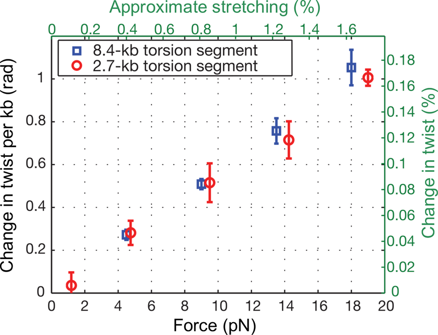
We found that an increase in extension of the molecule by 1% produced an increase in twist of 0.1%. To determine the value of the stretch-twist coupling parameter, at forces sufficient to suppress bending fluctuations (F >> kBT/P), we write the total energy of a DNA/magnetic bead system in which the molecule has been extended by an amount x beyond its contour length L and twisted by the amount ϕ, from its unperturbed equilibrium position, as:

We can then minimize this expression with respect to the angle ϕ, while holding the stretching x of the molecule and the torque τ applied to it constant:
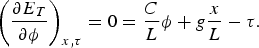
This expression gives the angle ϕ that minimizes the total energy for a given imposed extension x. Then:

Analysis of the experimental data gave a value of g =−90 ±20 pN⋅nm. This result showed that the value previously accepted for this parameter was not only wrong, but it had the wrong sign. The molecule overwinds when stretched, and this was indeed the title we chose for Jeff Gore's paper (Gore et al., Reference Gore, Bryant, Nollmann, Le, Cozzarelli and Bustamante2006).
How could we reconcile the negative twist-stretch coupling with the fact that DNA is known to unwind partly as it adopts the overstretched S-form under forces around 65 pN? Thus, to look for the change in sign of g at high tensions, we monitored the rotor bead as we gradually applied increasing magnetic force. We found that as the force rises and the extension of the DNA increases, the twist also increases – until the critical force of 30 pN is reached. Beyond this force, the molecule begins to unwind, as expected (Gore et al., Reference Gore, Bryant, Nollmann, Le, Cozzarelli and Bustamante2006).
The negative value of the twist-stretch coupling parameter observed below 30 pN implies that the molecule should lengthen if overwound. To estimate the magnitude of this effect we now write the total energy of the molecule/magnetic bead system as:

We can now minimize this expression with respect to the stretching x while we hold the twist and the force, F, constant:

Thus, the value of x* that minimizes the total energy of the system is then:

From this expression we obtain:

Given the value of −90 ± 20 pN⋅nm and the value of the stretch modulus of 1100 ± 200 pN determined previously, we expect that for each rotation in the overwinding direction, the molecule will lengthen by about 0.5 ± 0.1 nm. We tested this prediction by using again a torsionally constrained single DNA molecule attached to a glass surface on one end and to a magnetic bead on the other. Those experiments confirmed the predicted increase in length with each added turn of the magnetic bead using a rotating magnet (Gore et al., Reference Gore, Bryant, Nollmann, Le, Cozzarelli and Bustamante2006).
To rationalize the negative twist-stretch coupling parameter, we noted that a helix with a fixed backbone length and fixed radius must necessarily unwind as it is stretched. However, the DNA molecule is made up of a stiff phosphodiester backbone arranged on the surface (its solvent-exposing side) and a softer inner core. As the molecule is stretched, the tendency of the backbone to conserve its length and of the inner core to deform can result in a decrease of diameter of the latter and an increase in the number of turns of the former around the helix axis, as shown in Fig. 9. In such a model, the molecule overwinds when stretched and is no longer an isotropic rod.
At low force regime (⩽30 pN), stretching generates an overwinding of the helix because the inner core decreases in diameter as it is stretch. The outer helix is then able to wrap a larger number of times over the length of the molecule. Figure adapted and reprinted with permission from Gore et al. (Reference Gore, Bryant, Nollmann, Le, Cozzarelli and Bustamante2006).

Mechanical melting of DNA
In 1997, Heslot and collaborators used a microneedle to mechanically exert force and unzip the strands of a λ-DNA molecule. Typical unzipping forces were in the range of 10–15 pN and were related to the local GC and AT content of the molecule (Essevaz-Roulet et al., Reference Essevaz-Roulet, Bockelmann and Heslot1997). The spatial and temporal resolution of the experiment was improved later on by the same group using an optical trap (Bockelmann et al., Reference Bockelmann, Thomen, Essevaz-Roulet, Viasnoff and Heslot2002).
The approach of mechanically unzipping DNA allowed Michelle Wang and her collaborators to estimate the energy of interaction of DNA with the histone octamer. These authors determined the modification of the unzipping pattern of the DNA molecule by the presence of the histone components (Shundrovsky et al., Reference Shundrovsky, Smith, Lis, Peterson and Wang2006). In a later publication, Wang and collaborators applied a constant force to the ends of a histone-DNA complex and determined the residence time of the advancing fork as it progressed over the protein core. These residence times provided a measure of the strength of the protein–DNA interactions at those positions (Hall et al., Reference Hall, Shundrovsky, Bai, Fulbright, Lis and Wang2009). This same approach has been used by Ariel Kaplan and collaborators to study how the binding of a transcription factor with multiple zinc finger motifs is modulated by the sequence and context of its target sites (Rudnizky et al., Reference Rudnizky, Khamis, Malik, Squires, Meller, Melamed and Kaplan2018).
Traditionally the free energy associated with the base pairing and stacking interactions in dsDNA has been estimated using thermal denaturation. In 2010, Félix Ritort and collaborators showed that it is possible to determine the free energies of the 10 possible combinations of nearest-neighbor base pairs (NNBP), by mechanically unzipping a single DNA molecule (Huguet et al., Reference Huguet, Bizarro, Forns, Smith, Bustamante and Ritort2010). As the strands of the molecule are pulled apart, these authors observed reversible and reproducible force-extension transitions in the form of a saw-tooth pattern, that are correlated with the DNA sequence. This method allowed the authors to determine the free energies with a precision of 0.1 kcal mol–1 and to investigate the ionic strength dependence of these values. Félix and his collaborators further adapted the mechanical unzipping protocols to experimentally derive the NNBP free energies for RNA in sodium and magnesium salt conditions (Rissone et al., Reference Rissone, Bizarro and Ritort2022).
To summarize, the application of force spectroscopy methods to single molecules of DNA has resulted in the precise measurement of the molecule's mechanical properties, provided a rigorous test of theories of polymer elasticity, allowed the characterization of stress-induced extreme states of the molecule, and, as will be seen in section ‘Molecular motors’, established the conceptual and experimental basis for the design and analysis of mechanical assays of enzymes that act on DNA.
Folding studies
The studies of DNA elasticity taught us that it was possible to design experiments in which forces in the range of 0.1–100 pN could be controlled and used to investigate the mechanical behavior of polymers. But could we use these same approaches to study macromolecules organized in specific three-dimensional structures, like proteins and RNA? We wished to investigate and establish force as a controllable denaturant agent of these structures and to determine if the mechanical unfolding of these structures occurred in a single step or by populating one or more intermediate states, or if the molecules could be unfolded and refolded in a reversible manner.
RNA folding
Our single-molecule RNA folding studies arose from some discussions that Nacho Tinoco and I (C.B.) had prior to writing an article for the Journal of Molecular Biology in 1999 (Tinoco and Bustamante, Reference Tinoco and Bustamante1999). The motivation to understand RNA folding, we wrote, was based in the ever-expanding functionality of RNAs in the cell which includes being information carriers, scaffolds for complex nucleoprotein structures, adapters in translating the nucleotide code into the amino acid code, as ribozymes that catalyze self-splicing or peptide bond formation, as regulators of gene expression functioning in trans, or as regulators of transcription and translation acting in cis. To understand this large repertoire, we need to characterize RNA structure, how is it attained, how is it maintained, and what factors stabilize or destabilize it. In that article, ‘How RNA folds,’ we reasoned that the RNA folding problem should be an easier problem to ‘solve’ than its protein counterpart for several reasons. First, only 4 building blocks make up RNA as opposed to the 20 amino acids required for building proteins. Second, the ‘rules of engagement’ among these units are much simpler in RNA than in proteins as they mainly involve the canonical Watson–Crick and a few non-Watson–Crick base pairing of purines and pyrimidines. Moreover, these base pairing rules are strong and dominate the molecule's self-interactions. Third, only four basic secondary structure elements exist in RNA (helices, junctions, bulges, and loops). The helices mainly adopt A-form double helical structures, whereas the loops, bulges, and junctions are stabilized by non-Watson–Crick interactions and are bound by one or more helices. Fourth, while the stability of secondary structural elements in proteins depends on the tertiary structural context into which they fold, secondary structures of RNA are much less dependent of their tertiary folding context and can be predicted from thermodynamic data on base pairing and stacking interactions. The contextual nature of secondary structures in proteins results from the fact that the energies that stabilize these elements in proteins are comparable to those involved in their tertiary interactions. Thus, the formation of secondary structure depends on the nature of the tertiary folding contacts, and vice versa. One important corollary of this fact is that the energetic contributions of secondary and tertiary interactions in proteins are not separable. In the case of RNA, by contrast, the energy of the molecule can be written as the sum of the contributions of secondary interactions, those of tertiary interactions, and a significantly smaller term corresponding to the ‘interference’ between secondary and tertiary structures. An important task in the RNA folding problem is the characterization of these contributions during folding and unfolding.
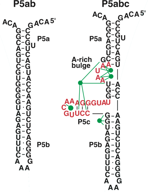
In 2000 Jan Liphardt and Bibiana Onoa came to Berkeley as joint postdoctoral fellows between Nacho Tinoco's laboratory and mine. We agreed that we would initiate the single-molecule RNA folding studies by comparing the folding of the P5abc domain of the Tetrahymena thermophila ribozyme with that of a simple hairpin derived from it that we termed P5ab.
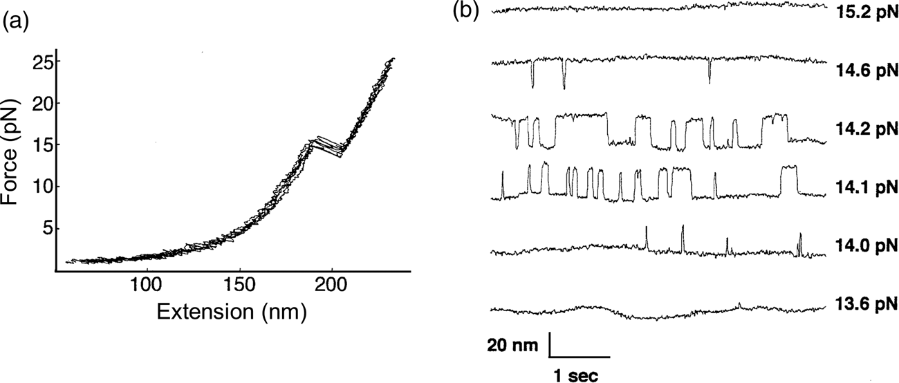
The P5abc domain contains a three-helix junction and can bind Mg2+ ions via an A-rich bulge to attain tertiary structure. In contrast the P5ab can only form secondary structure (Fig. 10). The individual RNA molecules were attached to polystyrene beads by RNA/DNA hybrid ‘handles.’ One bead was held by suction atop a micropipette and the other in a force-measuring optical trap. We moved the pipette relative to the trap at a constant speed to increase the force exerted on the molecules. With the P5ab hairpin, the force increased monotonically displaying the elastic response of the double-stranded handles until a sudden lengthening of the tether was observed between 14.0 and 15.5 pN (Liphardt et al., Reference Liphardt, Onoa, Smith, Tinoco and Bustamante2001) (Fig. 11a). The lengthening of 18 nm was consistent with the complete unfolding of the RNA molecule. By moving back the pipette, we let the molecule refold. Forward and reverse curves nearly coincided, indicating that the process occurred quasi-statically and at equilibrium (Fig. 11a). This observation implies that the work done to unfold and to refold P5ab (the area under the force versus extension curve in the transition region) is reversible. This reversible work is the potential of mean force, and it is equal to the free energy of folding.
Sequence and secondary structure of the P5ab and P5abc RNAs. The five green dots represent magnesium ions that mediate tertiary interactions (green lines) with groups in the P5c helix and the A-rich bulge. Figure adapted and reprinted with permission from Liphardt et al. (Reference Liphardt, Onoa, Smith, Tinoco and Bustamante2001).
(a) Force-extension curves for the unfolding of P5ab RNA in 10 mM Mg2+. The stretching and relaxing curves superimpose; the lack of hysteresis indicates that the unfolding is reversible. The proof of reversibility is shown in panel (b). When the force is held constant at the folding transition, the RNA switches back and forth with time from folded hairpin to unfolded single strand. The equilibrium constant K for the transition is obtained from the total time spent in each conformation; K is close to 1 at 14.1 and 14.2 pN. The rate constants for the forward and back reactions are obtained from the inverse of the average times spent in each conformation. Reprinted with permission from Tinoco and Bustamante (Reference Tinoco and Bustamante2002).
The kinetic data shown in Fig. 11b clearly display a change in folding/unfolding state lifetimes and thus transition rates as the force applied to the P5ab RNA varies. Box 1 describes the basic expressions of thermodynamics and kinetics modified to treat the case of molecules under the effect of force. For the P5ab unfolding transition, x B is equal to 20.2 nm, and x A corresponds to the distance between the two ends of the stem (i.e., the diameter of the folded RNA helix) and is equal to 2.2 nm, therefore Δx = 18 nm. Also, F 1 = 15.5 and F 2 = 14 pN (see Fig. 11a). We can use Eq. (15) to obtain a value of ΔG 0(F = 0). The integral can be evaluated following the WLC expression for the force required to extend the unfolded molecule and using Eq. (1), with a persistence length of 1 nm and a contour length of 0.59 nm⋅nt−1. This analysis gives a value of 157 ± 20 kJ⋅mol−1, which is in reasonable agreement with values obtained in bulk. However, this value will depend on the ionic strength of the medium and the concentration of divalent cations such as Mg2+.
Thermodynamics and kinetics expressions for single-molecule force spectroscopy
Consider the following reaction:

In an energy diagram such as shown in Fig. 12, A and B are states (folded and unfolded, e.g.) that occupy local free energy minima at positions xA and xB along the mechanical coordinate, so Δx = xB−xA. Then the free energy difference at zero force between A and B is (Bustamante et al., Reference Bustamante, Chemla, Forde and Izhaky2004):

where ΔG o is the standard free energy of the reaction at zero force, kB is the Boltzmann constant, T is the absolute temperature, and [A] and [B] are probabilities of occupation. To a first approximation, a force tilts the free energy surface along the mechanical coordinate by an amount linearly dependent on the distance on this coordinate, i.e.,

Here, the force F is the mid force of the transition, i.e., (1/2)⋅(F 1 + F 2). If the system is allowed to equilibrate between states A and B, then ΔG(F) = 0, and

Thus, the equilibrium constant of the unfolding reaction depends exponentially on the force that shifts the populations of states A (folded) and B (unfolded). Now, strictly speaking, the positions of the minima in the energy surface also change with the applied force. That is, in general, force not only tilts the energy surface but also shifts the minima and maxima. This shift depends on the local curvature of the potential energy at these extremes. The stiffer the potential the more ‘localized’ the state and the lesser the shifting effect of force. Because the free energy of the reaction A↔B must be measured between the new energy minima, Eq. (14) must be corrected by the small energy shift due to this change in minima position (see Fig. 12):

where ${\rm \Delta }G_{{\rm stretch}}^{A\to B} ( F ) = {\rm \Delta }G_{{\rm stretch}, B}-\;{\rm \Delta }G_{{\rm stretch}, A} = \int_{x_B( {F = 0} ) }^{x_B( F ) } {Fdx} -\int_{x_A( {F = 0} ) }^{x_A( F ) } {Fdx}$ . That is, this term represents the difference in free energy due to the shift of the minima at states A and at B. In most unfolding reactions, the folded state is quite rigid and only the unfolded state is compliant and contributes to this term. If both states have the same curvature, their minima are shifted by the same amount and ${\rm \Delta }G_{{\rm stretch}}^{A\to B} ( F )$
 = 0. Equation (15) shows that the standard free energy difference of the reaction at zero force, ΔG o, is the reversible work at a given force F minus the effect due to the shift in populations between states A and B under the applied force and minus the difference in free energies of stretching products and reactants at that force (Tinoco and Bustamante, Reference Tinoco and Bustamante2002).
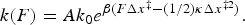
The force dependence of rate constants k(F) results from the fact that the application of force not only affects the heights and positions of the folded and unfolded states along the reaction coordinates but also the relative height of the barrier separating them (Fig. 12). Bell (Reference Bell1978) was the first to phenomenologically describe such an experimental dependence of the rate constant on the external force by introducing a –FΔx factor in the classic reaction kinetics Arrhenius equation:

where A is the attempt frequency of the transition, k 0 is the folding/unfolding rate at zero force, equal to $Ae^{-\beta {\rm \Delta }G^{\ddagger} }$ , β = 1/kBT, Δx‡ is the distance to the transition state (positive from the folded to the unfolded state, and negative in the reverse direction), and ΔG‡ is the apparent free energy of activation at zero force. According to Eq. (16) a plot of the natural logarithm of the rate coefficient versus the applied force should give a straight line with negative slope for the folding rate and a positive slope for the unfolding rate, analogous to the Chevron plots obtained in ensemble kinetic studies where chemical denaturants are used to unfold proteins. Furthermore, the slopes of the fitted lines yield the corresponding distances to the transition state (see examples in section ‘Co-translational folding’ on co-translational protein folding). Since the shape (curvature) of the transition barrier is also modified by the external force, additional corrections can be made by accounting for the local stiffness, κ, of the potential:
The simple-to-apply Bell's model, however, begins to deviate when the potential energy surface becomes more complex. Based on Kramers' theory (Kramers, Reference Kramers1940) of diffusion over a barrier, Dudko et al. (Reference Dudko, Hummer and Szabo2006) incorporated in the Bell equation a scaling factor ν to specify the nature of the underlying free-energy barrier profile, thus establishing a theoretically rigorous and yet generalized framework to describe the force-dependent kinetic rates as follows:

ν = 1/2 corresponds to a harmonic well with a cusp-like barrier, whereas ν = 2/3 corresponds to a linear-cubic free energy surface and an adequate correction for most potentials encountered in RNA and protein folding studies. When ν = 1 the Bell equation is recovered. As long as a broad enough force range is explored when measuring the transition rate, Dudko's formula allows us to extract not only k 0 and Δx‡ but also ΔG‡ without varying the temperature of our experiments. Given that the above expressions of force-dependent rate constant k(F) and equilibrium constant Keq(F) are completely general and valid for RNA and protein folding studies, we can directly determine many features of their folding energy landscapes from the single-molecule force spectroscopy measurements.
The effect of force on the free energy of a two-state system, where x represents the mechanical reaction coordinate. Black solid curve: no force perturbation. Red solid curve: after applying a positive force (blue line) to the system (dashed curve). The application of force lowers the energy of both the transition state ‡ and state B relative to state A (ΔG 0‡ and ΔG 0), which increases the rate of the forward reaction and the population of state B, respectively. The positions of the free energy minima (xA and xB) and maximum (x ‡) shift to longer and shorter x, respectively, with a positive applied force. Their relative shifts in position depend on the local curvature of the free energy surface and the corresponding free energy change of states A and B upon stretching is ΔG stretch. Reprinted with permission from Bustamante et al. (Reference Bustamante, Chemla, Forde and Izhaky2004).
Interestingly, when the force applied to the P5ab RNA was held at or near the midpoint of the transition, the molecule displayed bi-stability, folding and unfolding reversibly. By increasing the pre-set force, we could tilt the equilibrium toward the unfolded state and thus directly control the thermodynamics and kinetics of RNA folding in real time (Fig. 11b). The average life-time of the molecule in the unfolded and the folded states gives the inverse of the rate constant for folding and unfolding respectively, at that force. This rate can be extrapolated to zero force (see Box 1) and their ratio can be used to calculate the equilibrium constant at zero force and from that the corresponding standard free energy. The value obtained was 156 ± 8 kJ mol−1.
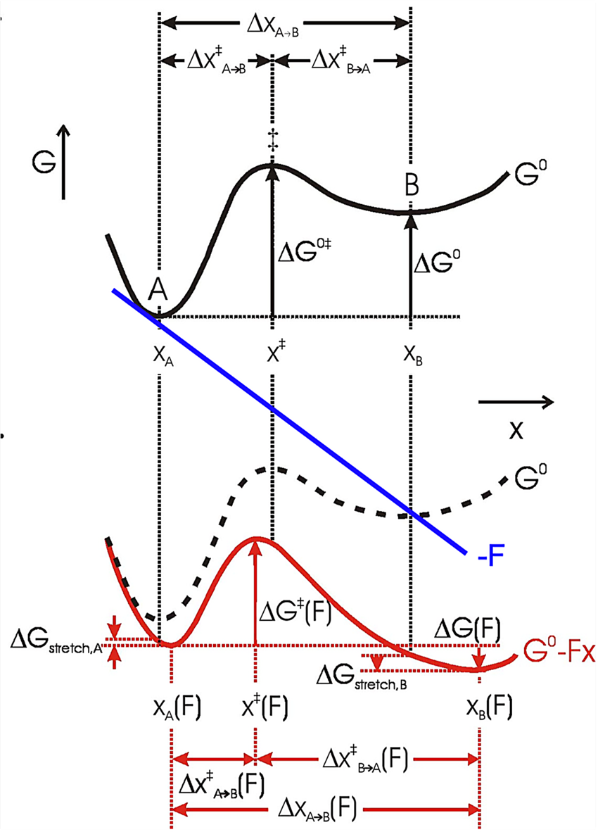
In contrast to the reversible unfolding of P5ab, the force extension curves corresponding to the mechanical unfolding and refolding of P5abc in the presence of Mg2+ display marked hysteresis (Liphardt et al., Reference Liphardt, Onoa, Smith, Tinoco and Bustamante2001), with the force at which RNA unfolds during pulling being larger than that at which it refolds during relaxation (see green curves in Fig. 13). In these conditions, the molecule is known to adopt a tertiary structure. Forces as high as 22 pN are required to unfold the molecule. In some of the force-extension curves the molecule was observed to unfold and refold through an intermediate (see Fig. 13a), which was identified as the molecule having the P5b helix at the base of the hairpin unfolded. Upon removal of the Mg2+, the molecule regains its ability to fold reversibly with little hysteresis (Fig. 13b). This observation indicates that the formation of the tertiary structure in the presence of the divalent cation involves the crossing of a significant energy barrier that greatly slows down the folding and unfolding rates relative to the rate of pulling, giving rise to the hysteresis observed.
(a) Stretch (blue) and relax (green) force-extension curves for P5abc RNA (right; see also Fig. 10) in 10 mM Mg2+. Inset: detail of P5abc stretching curves showing unfolding intermediates (red stars). (b) Comparison of P5abc force extension curves in the presence and absence of Mg2+. Reprinted with permission from Liphardt et al. (Reference Liphardt, Onoa, Smith, Tinoco and Bustamante2001).
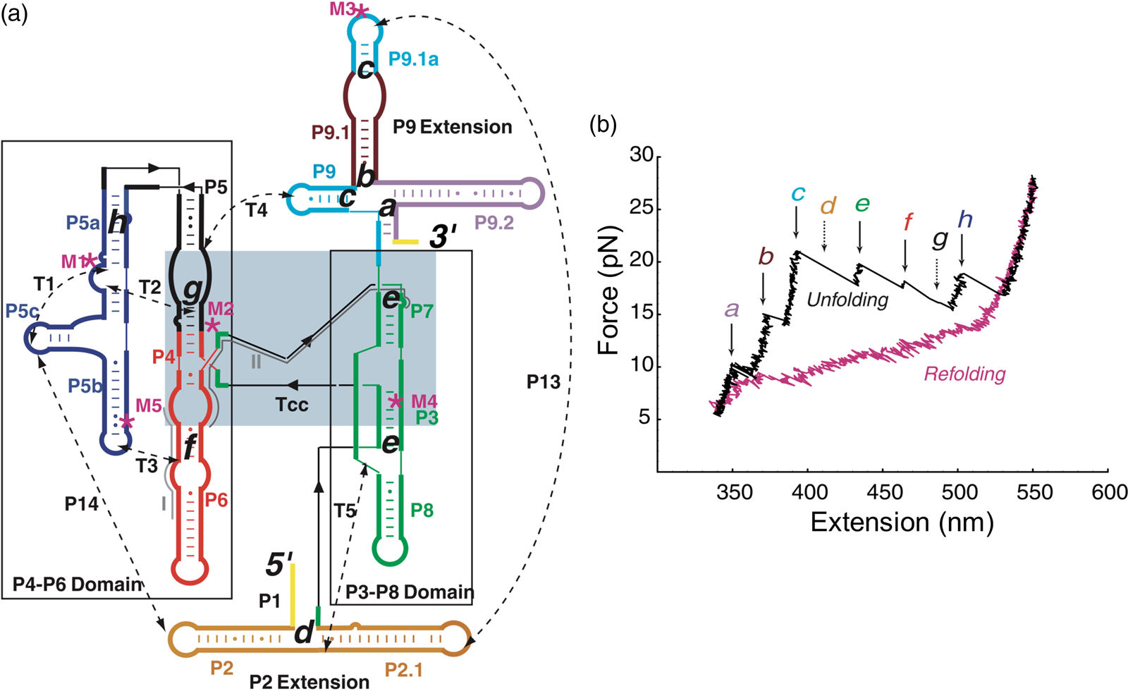
Having succeeded in studying the mechanical unfolding and refolding of a simple domain of the T. thermophila group I intron ribozyme, Bibiana Onoa and Sophie Dumont, then a graduate student in the laboratory, decided to tackle the challenging task of characterizing the unfolding/refolding intermediates of the L-21 derivative of this ribozyme, a 390-nt catalytic RNA whose three-dimensional structure, independently folding domains, and intra and inter-domain contacts were already known (Fig. 14a). The force-extension unfolding curves of this molecule reveal 8 different intermediaries (Fig. 14b). In a veritable tour-de-force, Bibiana and Sophie set themselves to annotate and identify the nature of each intermediate state. Developing mutants to destabilize certain secondary and tertiary contacts, using oligonucleotides to passivate other contacts, and taking advantage of the modular nature of RNA folding which allowed them to characterize some of the domains in isolation, they were able to painstakingly identify and annotate each of the intermediates.
(a) Secondary structure of the L-21 ribozyme. The two main domains, P4-P6 and P3-P8, are boxed; a light blue box indicates the catalytic core, Tcc. Dashed lines are tertiary contacts and base-paired regions; ‘M’ labels are site-directed mutations. The letters a to h indicate the proposed positions of the kinetic folding barriers. (b) Representative unfolding (black) and refolding (pink) force-extension curves of the L-21 RNA displaying six unfolding events (rips, a to h). Experiments were done at 298 ± 2 K in 10 mM Tris-HCl (pH = 7), 250 mM NaCl, and 10 mM MgCl2. The rips correlate to the unfolding of domains and subdomains shown in (a). The unfolding curve chosen here does not display barriers d and g, indicated by the dashed arrows. Reprinted with permission from Onoa et al. (Reference Onoa, Dumont, Liphardt, Smith, Tinoco and Bustamante2003).
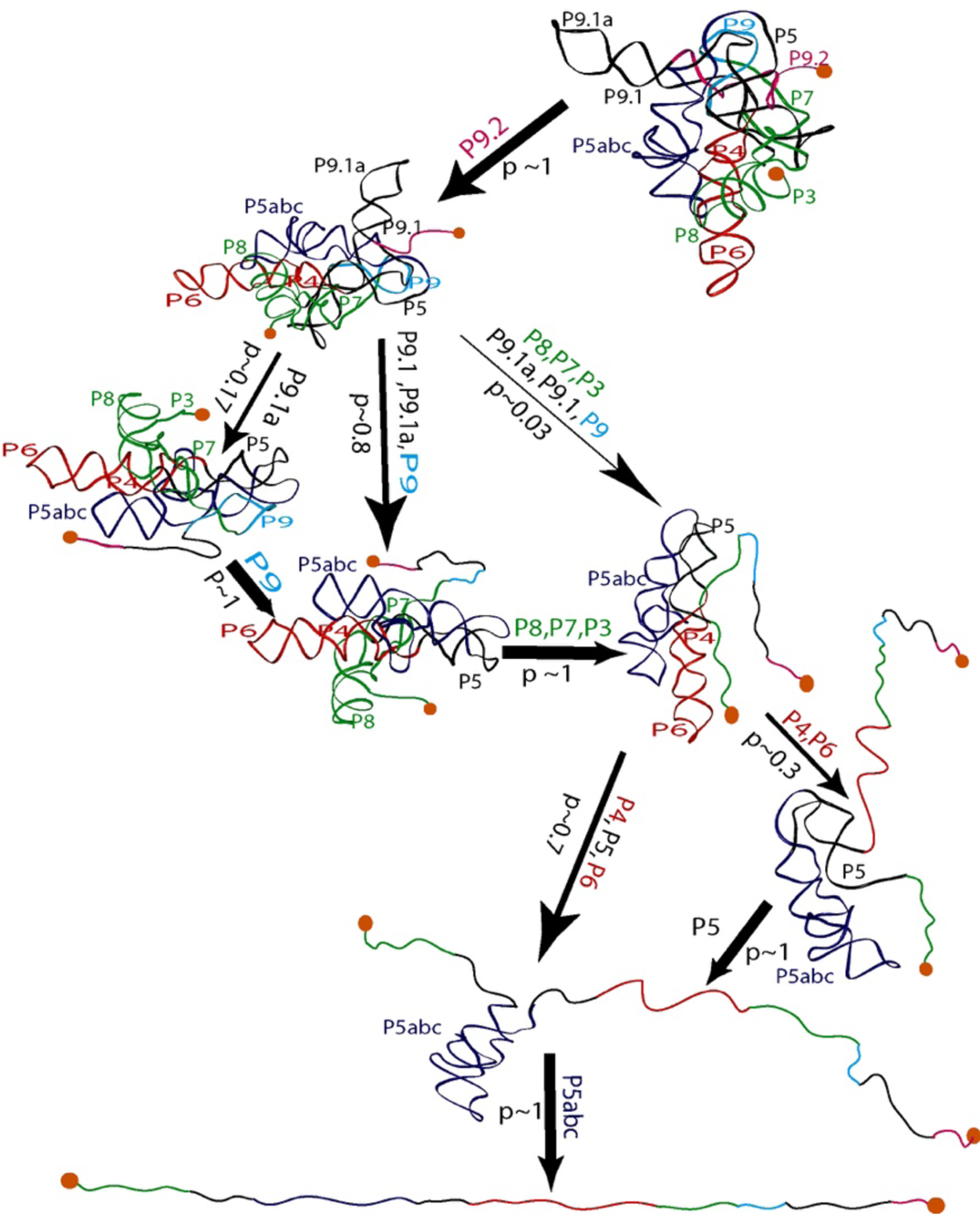
Seeing the richness of the force-extension curves, I told Bibiana that she should obtain a hundred of these curves in order to establish the alternative unfolding paths of the molecule. Bibiana is from Colombia, and I am from Peru, but we used English to communicate in the laboratory. My Spanish accent must have been responsible for her understanding that I had said not ‘a hundred’ but ‘eight hundred’ curves. Three weeks later, Bibiana showed in my office and told me: ‘Well you said eight hundred, but I have obtained nine hundred.’ Because of this small error in our communication, Bibiana ended up acquiring more than sufficient statistics enabling her to determine not only the unfolding intermediates but also the probability that the molecule would visit these states in any given trajectory from the folded to the unfolded state. Figure 15 depicts the molecular trajectory of unfolding the L-21 ribozyme without the small P1 and P2 domains. Clearly the molecule can traverse multiple trajectories in its transition from the fully folded to the completely unfolded state, and certain intermediates are more frequently adopted among all the attainable states identified (Onoa et al., Reference Onoa, Dumont, Liphardt, Smith, Tinoco and Bustamante2003).
Mechanical unfolding pathway of the L-21 ribozyme (Onoa et al., Reference Onoa, Dumont, Liphardt, Smith, Tinoco and Bustamante2003). The domains/subdomains (same nomenclatures as in Fig. 14A) sequentially unfolded at each step are indicated next to each arrow, whose thickness reflects the flux/probability (p) for the corresponding unfolding transition to occur.
More recently, as the temporal resolution of these measurements improved to tens of μsec, Michael Woodside and collaborators (Neupane et al., Reference Neupane, Foster, Dee, Yu, Wang and Woodside2016; Neupane et al., Reference Neupane, Wang and Woodside2017) were able to directly discern the time required for a biomolecule to diffuse across the transition state barrier that dominates the folding kinetics (recall Kramers' in Box 1). This transition path time is largely set by the conformational diffusion coefficient, D, which reflects some details of the energy landscape – such as the roughness around the barrier – and the level of internal friction in the molecule that undergoes the folding transition. Unlike folding rates (k), however, the average transition path time (τ tp) is far more sensitive to D than to barrier height (${\rm \Delta }G^{\ddagger}$ ) (Chung and Eaton, Reference Chung and Eaton2013; Chung et al., Reference Chung, Piana-Agostinetti, Shaw and Eaton2015), and was measured to be 1000-times shorter than the lifetimes of the unfolded and folded states for a DNA hairpin (Neupane et al., Reference Neupane, Foster, Dee, Yu, Wang and Woodside2016). Furthermore, they found that the shapes of the transition-time distributions for unfolding and refolding are identical – as expected from the time-reversal symmetry of the folding transitions – and that the broad distribution with a long exponential tail is consistent with theoretical models assuming simple 1D diffusion over a harmonic barrier for folding processes.
Co-transcriptional RNA folding
Steven Block and collaborators showed that it is possible to grab the nascent RNA chain off the surface of an active RNA polymerase to follow its co-transcriptional folding in real-time. They applied this assay to investigate the co-transcriptional folding of pbuE adenine riboswitch, which can attain alternative RNA folds in an adenine-concentration-dependent manner to regulate adenine efflux from the cell. Specifically, they monitored the co-transcriptional folding of an anti-termination adenine-bound aptamer, which is rather short-lived but lasts long enough to block RNA polymerase from termination, thereby completing the full transcript. Hence, the adenine-bound aptamer, thermodynamically less favorable than the alternative terminator long hairpin fold, is able to control kinetically the fate of the transcript during active transcription (Frieda and Block, Reference Frieda and Block2012). In our laboratory using a similar experimental design, two postdoctoral fellows, Shingo Fukuda and Shannon Yan, showed that the signal recognition particle RNA (SRP RNA) exhibits a robust co-transcriptional folding invariant to transcription rates, and that it attains a non-native obligatory intermediate fold during its synthesis. Shannon further characterized that this obligatory intermediate in fact permits sequence maturation by RNase P on the nascent SRP RNA during early transcription, which possibility was not known before. Yet, she found that RNA mutations stabilizing the intermediate impede folding transitions toward the final native long-hairpin fold of SRP RNA, hence rendering a fatal loss of function that impacts Escherichia coli cell viability (Fukuda et al., Reference Fukuda, Yan, Komi, Sun, Gabizon and Bustamante2020).
Protein folding studies
In 1996, Steve Smith and I (C.B.) attended a Biophysical Society Meeting in New Orléans where we met Miklós Kellermayer. At the time he was a postdoctoral fellow in Henk Granzier's laboratory at Washington State University. Miklós and Henk studied muscle physiology and were interested in understanding the function of the giant muscle protein titin, a 3.5-MDa polypeptide containing a linear array of ~300 immunoglobulin C2 (Ig) and fibronectin type III (FNIII) domains, which spans the half-sarcomere, from the Z line to the M line. This protein, also known as connectin, is responsible for the generation of ‘passive force,’ which is generated when the muscle fiber is stretched and for the generation of the restoring force after sarcomere contraction. Thus, titin function is to maintain the structural integrity of the sarcomere in actively contracting muscle. Miklós, Henk, Steve, and I agreed to collaborate and investigate the mechanical properties of this protein by tethering it between two beads, one held in an optical trap and the other atop a movable micropipette (Kellermayer et al., Reference Kellermayer, Smith, Granzier and Bustamante1997).
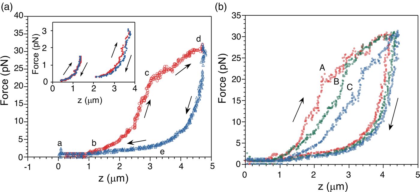
The force-extension curves displayed a smooth monotonic rise that we assigned to the extension of unfolded regions and the alignment of the globular domains in the titin molecule (Kellermayer et al., Reference Kellermayer, Smith, Granzier and Bustamante1997). Between 20 and 30 pN the molecules undergo a structural transition that we identified as the unfolding of globular domains. Upon relaxation, the force-extension curve again decreases monotonically, and a shortening structural transition is observed at ~2.5 pN (Fig. 16a). The elastic behavior of the molecule displays marked hysteresis. A fit of the smooth regions of the relaxation curves to the WLC model yielded a persistence length of 20 Å. Interestingly, we found that the fraction of the molecule that refolded after successive pulling and relaxation cycles decreased steadily, indicating some kind of ‘wearing-out’ or ‘molecular fatigue’ resulting from the mechanical unfolding/refolding cycle (Fig. 16b).
(a) The force-extension (F-z) curve of a single titin molecule, with points (a to e) highlighted at the beginning and the end of the transitions. The rate of stretch (red) and release (blue) is ~60 nm s–1. Inset: F-z curves where the stretch or the release of titin was stopped short of entering the stretch or release transition (i.e., before point c and after point e, respectively) displaying no hysteresis, presumably because no unfolding has taken place at this point. (b) Effect of repetitive cycles of stretch and release (2nd cycle: A, red; 3rd cycle: B, green; 5th cycle: C, blue) in the absence of chemical denaturant; the stretch/release rate is 65 nm s–1. Reprinted with permission from Kellermayer et al. (Reference Kellermayer, Smith, Granzier and Bustamante1997).
The same week in which our work was published, two other reports on the mechanical manipulation of titin appeared. One also in Science by Herman Gaub and Julio Fernández using atomic force microscopy (Rief et al., Reference Rief, Gautel, Oesterhelt, Fernandez and Gaub1997), and another in Nature by the group of Robert Simmons using optical tweezers (Tskhovrebova et al., Reference Tskhovrebova, Trinick, Sleep and Simmons1997). It was a clear indication that increasing number of scientists were beginning to accept force spectroscopy as a viable method of biophysical analysis.
Julio Fernández's group has used extensively AFM-based nano manipulators to investigate the elasticity of titin. In this case, the molecule is usually deposited on a surface of freshly cleaved mica. At the beginning of an experiment, the surface approaches the tip-carrying cantilever to pick up a molecule from the mica. As the sample is retracted, tension is applied to the tethered molecule. The successive unfolding of the individual domains or monomers leads to sudden drops in force, resulting in a characteristic saw-tooth force rip pattern (Rief et al., Reference Rief, Gautel, Oesterhelt, Fernandez and Gaub1997). Since AFM cantilevers are usually 100–1000 times stiffer than optical tweezers, typical loading rates (i.e., the product of the stiffness of the cantilever and the rate of pulling) applied to the molecules in these experiments are much higher than in their optical tweezers counterparts and, accordingly, the molecules are often seen to unfold at 100 pN or above. The technique can also be used in a constant force mode (‘force clamp’) and when used with a molecule like titin or tandem repeats of globular proteins, it allows to observe the stepwise unfolding of the individual monomers as changes in extension as a function of time (Garcia-Manyes et al., Reference Garcia-Manyes, Brujic, Badilla and Fernandez2007).
DNA handles
Our initial study of protein folding had been possible because titin, with a contour length of ~1 μm, could be tethered with relative ease between two beads in the optical tweezers instrument. Tethering much smaller globular domains between the comparatively large beads required a sort of ‘molecular handles’ to connect the molecule of interest to the beads. I (C.B.) thought that segments of dsDNA were the obvious choice given the molecule's large persistence length and that by then the elasticity and other mechanical properties of DNA as a biopolymer have been properly characterized by my group and many other laboratories. Furthermore, it is biochemically feasible to make protein–DNA chimeras using various attachment schemes. Ciro Cecconi, then a graduate student in the laboratory, eventually succeeded in this task (Cecconi et al., Reference Cecconi, Shank, Dahlquist, Marqusee and Bustamante2008, Reference Cecconi, Shank, Marqusee and Bustamante2011).
With the DNA handles in hand, Ciro and a graduate student in Susan Marqusee's laboratory, Elizabeth Shank, set to study the mechanical unfolding of RNAase H. In these studies, we found that the molecule unfolds in a two-state manner and refolds through an intermediate that we interpreted as the formation of a transient molten globule-like structure since it displayed anomalously large compliance. We found a narrow range of forces in which the molecule hops between the unfolded and the intermediate. Occasionally hopping stopped as the molecule transitioned from the intermediate to the folded state. These folding events always occurred from the intermediate, indicating that this was an on-pathway intermediate. This kind of information is very hard to come by using bulk methods. In single-molecule spectroscopy it is a direct observable of the experiment. Our article appeared in 2005 (Cecconi et al., Reference Cecconi, Shank, Bustamante and Marqusee2005).
Ciro and Elizabeth also collaborated in the study of the mechanical unfolding/refolding of T4 lysozyme and showed that the N-terminus and C-terminus domains of the molecule unfold and fold cooperatively (‘all-or-none’ behavior) displaying a single rip and zip, respectively connecting the folded and the unfolded states, when subjected to force. Using mechanical force as the denaturant was essential to characterize the folding and unfolding cooperativity of these domains, because it allowed us to selectively unfold one domain of the molecule and determine the consequence in the other domain. We suspected that the coupling between the two domains is encoded in the topology of the polypeptide chain. Indeed, the molecule has a ‘re-entrant’ connectivity in which the first 12 amino acid residues located at its N-terminus in the primary structure adopt an alpha-helical structure (the A-helix) that is organized instead as part of the C-terminus domain in the tertiary structure. To test that this re-entrant connectivity is responsible for the folding coupling between the two domains, Ciro and Elizabeth generated a circular permutant that relocates these 12 residues after the C-terminus, thus eliminating the re-entrant topology. First, they confirmed that this permutant adopts the same structure and retains the stability and enzymatic activity of the initial molecule. Then, Ciro and Elizabeth showed that this circular permutant unfolds and refolds in two steps, with the intermediate corresponding to the folded C-terminus (Shank et al., Reference Shank, Cecconi, Dill, Marqusee and Bustamante2010). Thus, the reorganization of the molecule's topology (without changing its structure) in the permutant had led to the loss of the folding cooperativity between its domains, which now fold and unfold independently. To arrive at this conclusion, we needed to obtain the free energy of folding of the molecule from non-equilibrium experiments, for which we used for the first time the powerful fluctuation theorems of non-equilibrium statistical mechanics as described in section ‘Bridging equilibrium and non-equilibrium statistical mechanics: fluctuations theorems’ below.
Co-translational folding
In 2006 I (C.B.) visited the University of Texas Medical Branch to give an invited lecture, and I met Christian Kaiser, who at the time was looking for a postdoctoral fellowship to continue his doctoral studies on protein folding. Christian was really excited about the single-molecule studies I presented in that visit and approached me about the possibility of joining my laboratory. A few months later he moved to Berkeley, and we began to work together on co-translational protein folding. One crucial observation is that the rate of protein synthesis is slow compared to the rate of protein folding. Proteins are synthesized by the ribosome in a vectorial manner, that is, residues are added to the C-terminus one by one, and this is a relatively slow process, occurring at ~10–20 amino acids per second in fast growing bacteria, and considerably more slowly in eukaryotes. This slow synthesis rate inevitably leads to the exposure of hydrophobic chains to the aqueous solvent. Folding, on the other hand, can be very fast. Some small proteins fold within microseconds, and many fall in the range between 1 ms and 1 s. Very large proteins sometimes need a long time to reach their native structure, but the formation of intermediates or the folding of individual domains will be faster. It is therefore very likely that folding can begin before the entire sequence has been synthesized. Intuitively, this seems like a good strategy for multi-domain proteins: the first domain can fold before the next one is synthesized, and that avoids non-productive interactions between the unfolded domains. But what about the individual domains or small globular proteins? What conformations do they adopt while they are being synthesized? For example, T4 lysozyme is a small protein with 164 residues. At very fast elongation rates, it will take the cell, at the very least, 8 s to make this protein. During these 8 s, more and more of the sequence emerges from the ribosome. However, 8 s is a really long time for protein folding. We know from in vitro experiments that the full-length T4 lysozyme folds to its native state quite fast, at a rate of about 20 per second (Bremer and Dennis, Reference Bremer and Dennis2008). Then, what factors prevent the protein from adopting aberrant, trapped structures on the ribosome during synthesis? To answer this question, we must look at what happens to the nascent chains as they are being made. Does the ribosomal environment or the vectorial nature of the synthesis modify the folding pathway of the protein or their intermediates? These were the questions that Christian Kaiser and Daniel Goldman, a graduate student at the time, set together to address.
Our idea was to compare the folding of the full T4 lysozyme protein, with its de novo folding as it takes place during translation on the surface of the ribosome. This comparison is difficult to do with ensemble methods because we must follow the folding of a small protein in the context of the ribosome, which itself has more than 50 proteins and is more than 100 times larger. Therefore, it is difficult to employ spectroscopic methods commonly used in bulk folding studies such as circular dichroism, hydrogen exchange, and tryptophan fluorescence spectroscopy, to study co-translational folding. Moreover, we cannot use common denaturants, such as urea or elevated temperatures, because these agents will also affect the ribosome. Thus, we needed a way of selectively inducing the unfolding and following the refolding of the nascent chain. Ideally, we also wanted an approach that can resolve single-molecule events, so we could capture transiently populated and possibly heterogeneous states. We decided to grab an individual fully synthesized protein or its truncated versions, subject it to denaturation by force in solution, and compare its behavior to that of a fully or partially synthesized protein as it emerges on the surface of the ribosome with an in vitro reconstituted translation system (Fig. 17).
Experimental setup for optical tweezers measurements of ribosome-bound nascent proteins. A ribosome–nascent chain complex is tethered between two polystyrene microspheres via DNA handles. Attachment points are located on the large subunit of the ribosome and the N terminus of the nascent protein. The force applied to the assembly can be varied by moving the optical trap. Reprinted with permission from Kaiser et al. (Reference Kaiser, Goldman, Chodera, Tinoco and Bustamante2011).
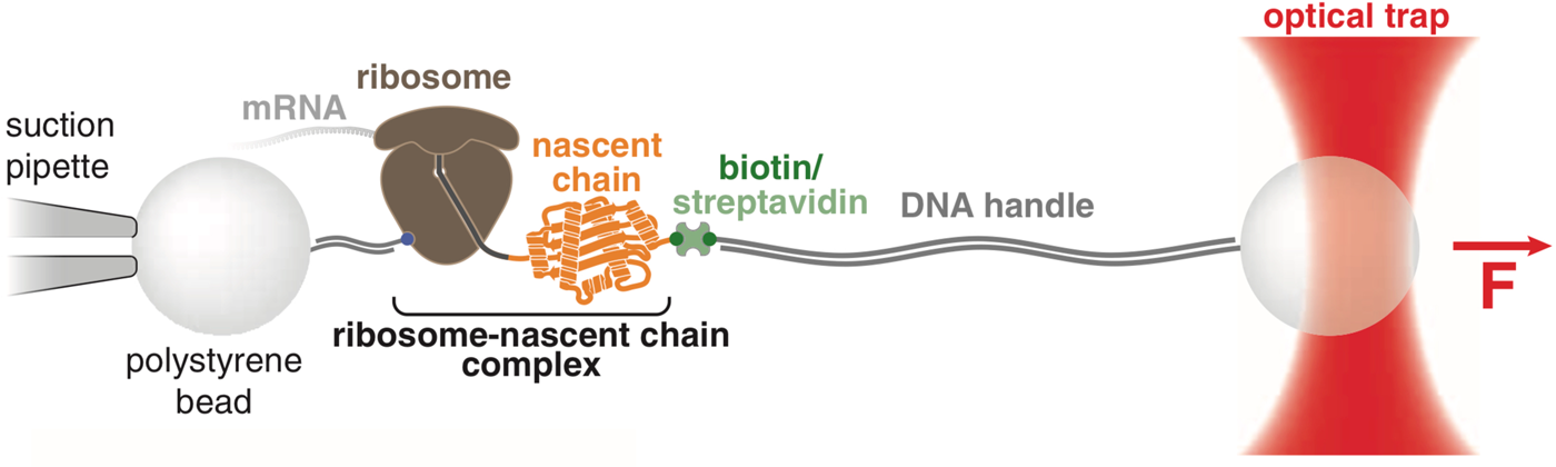
For the fully synthesized molecule we found that the ribosome does not affect the native state: the extension changes upon unfolding are very similar, indicating that the protein folds to the same native state regardless of whether it is free or ribosome-bound. We also found that the unfolding force-distribution for both proteins is very similar with a mean force of ~17 pN, indicating that the ribosome does not measurably destabilize the folded protein, and that unfolding likely occurs through the same pathway in both scenarios. In other words, the ribosome surface does not stabilize or destabilize the folded protein. However, unfolding is only half of the story. The other half, namely folding, is actually more interesting. We know that the protein folds after we relax the force, because when we pull repeatedly, we observe similar unfolding events. What we found is that while the protein in solution quickly refolded upon relaxation after being mechanically unfolded, the protein on the surface of the ribosome very often did not. We found that on the surface of the ribosome the protein refolding rate slows down more than 200 times, relative to its folding in solution. This was surprising to us. Statistical mechanics considerations (Zhou and Dill, Reference Zhou and Dill2001; Mittal and Best, Reference Mittal and Best2008) would instead predict that holding a polypeptide close to a surface decreases the number of its accessible conformations and should speed up folding. The protein was tethered to the ribosome via a 41-amino acid residue linker, long enough to span the ribosomal tunnel. When we extended this linker to provide more spacing between the folding protein and the ribosomal surface, we found that the rate of refolding of the protein increased and continued to do so as we lengthened the linker (Fig. 18), indicating that the interaction of the polypeptide with the surface of the ribosome was responsible for the slowing down of its folding. Moreover, we found that the effect was strongly ionic strength dependent. Increasing the ionic strength of the medium greatly decreased the folding slowdown, indicating that the interactions between the polypeptide and the ribosome were, at least in part, of electrostatic origin. Christian and Daniel were able to also identify the refolding step of T4 lysozyme that was slowed down by the ribosome. Next, we compared the mechanical unfolding and refolding of truncated versions of the protein in solution with their stalled translational counterparts outside the exit of the ribosome. Surprisingly, the truncated polypeptides displayed a very heterogeneous unfolding and refolding force distribution, indicating that each time these molecules were allowed to refold they adopted different misfolded states. However, the same molecules on the surface of the ribosome displayed no unfolding or refolding transitions. Somehow the ribosome surface prevented their misfolding. These results suggest that the surface of the ribosome is not inert; rather, it establishes interactions with the nascent chain that slow down or prevent its misfolding, maintaining it in a folding-competent conformation, and providing time for the rest of the domain or the protein to emerge from the exit tunnel. This work was published in 2011 (Kaiser et al., Reference Kaiser, Goldman, Chodera, Tinoco and Bustamante2011).
Apparent refolding rates for ribosome-bound T4 lysozyme with 41-amino acid (+41) and 60-amino acid (+60) linkers and for the free protein (free). Error bars: 95% CIs. Reprinted with permission from Kaiser et al. (Reference Kaiser, Goldman, Chodera, Tinoco and Bustamante2011).
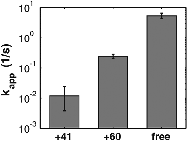
While the co-translational folding of a single-domain protein is decelerated through interactions with the ribosome surface to avoid non-native contacts within the nascent polypeptide chain before the protein is fully synthesized, we wonder how the folding of a multi-domain protein is modulated during active translation. Hence, a recent graduate student Lisa Alexander went on to investigate the real-time co-translational folding pathway of calerythrin, a two-domain calcium-binding protein from the bacterium Saccharopolyspora erythraea (Swan et al., Reference Swan, Hale, Dhillon and Leadlay1987; Tossavainen et al., Reference Tossavainen, Permi, Annila, Kilpelainen and Drakenberg2003). Calerythrin contains four EF hands, each has a helix-loop-helix motif with a calcium-binding site in the loop; the first and second pairs of hands (EF1 + 2 and EF3 + 4) form the N- and C-domain of the protein, respectively. Lisa first found that, under equilibrium conditions (i.e., an isolated protein off the ribosome or as a stalled ribosome-bound nascent chain complex, RNC, that has been allowed to equilibrate), the folding of full-length calerythrin (EF1-4) always proceeds through a C-terminal intermediate, and the N-domain folds last. Given that in solution the C-domain is an obligatory intermediate for productive folding of calerythrin, we wondered whether the vectorial N-to-C nature of protein synthesis on the ribosome forces the protein to fold first through the N-terminus domain. Lisa found that while the N-domain alone, off the ribosome, folds at rates of 600 ± 370 s−1, it does not fold when it emerges on the surface of the ribosome. When she incrementally extended the construct to include EF1 + 2 + 3, she found that off the ribosome, the N-domain does not fold and instead, adopts a misfolded state where EF3 mis-pairs with EF1, replacing EF2. When EF1 + 2 + 3 is allowed to emerge out of the ribosome, the stalled nascent chain also adopts the misfolded state observed off the ribosome. Following the Bell's model discussed earlier (see Box 1), Lisa was able to extract the misfolding kinetics of EF1 + 2 + 3 and compare those rates on and off the ribosome (see Chevron plot in Fig. 19, where the y-axis depicts the natural logarithm of the rates, and the x-axis the force applied to the nascent chain). She found that even though the nascent chain misfolds, the ribosome in fact decelerates the misfolding rate by 104-fold and accelerates the unfolding rate to escape the misfolded state by 90-fold (extrapolated at zero force) compared with the E1 + 2 + 3 off the ribosome. However, the time required for EF1 + 2 + 3 to misfold on the ribosome at zero force is still quite short (6 ± 3 × 10⁻⁴ s), and the time it remains misfolded is still very long (1.9 ± 0.5 s). Hence, under a typical rate of protein synthesis (4–6 s−1 at room temperate to match our experimental conditions) (Zhu et al., Reference Zhu, Dai and Wang2016), the data derived from the stalled nascent chains data would seem to indicate that the intermediate nascent chain EF1 + 2 + 3 would readily misfold during active translation, despite the relative destabilization by the ribosome.
The misfolded state has altered kinetics on the ribosome. (a) Overlaying the refolding curves from RNC177 in which all of the N-domain is out of the tunnel, but part of the C-domain is still in it (magenta) and EF123 (black) shows they are the same size transition, which corresponds to full misfolding. (b) The folding kinetics of RNC177 are slower and the unfolding kinetics are faster relative to EF123. Diamonds: unfolding rates, circles: folding rates. Error bars, standard error (SE). Figure adapted and reprinted with permission from Alexander et al. (Reference Alexander, Goldman, Wee and Bustamante2019).
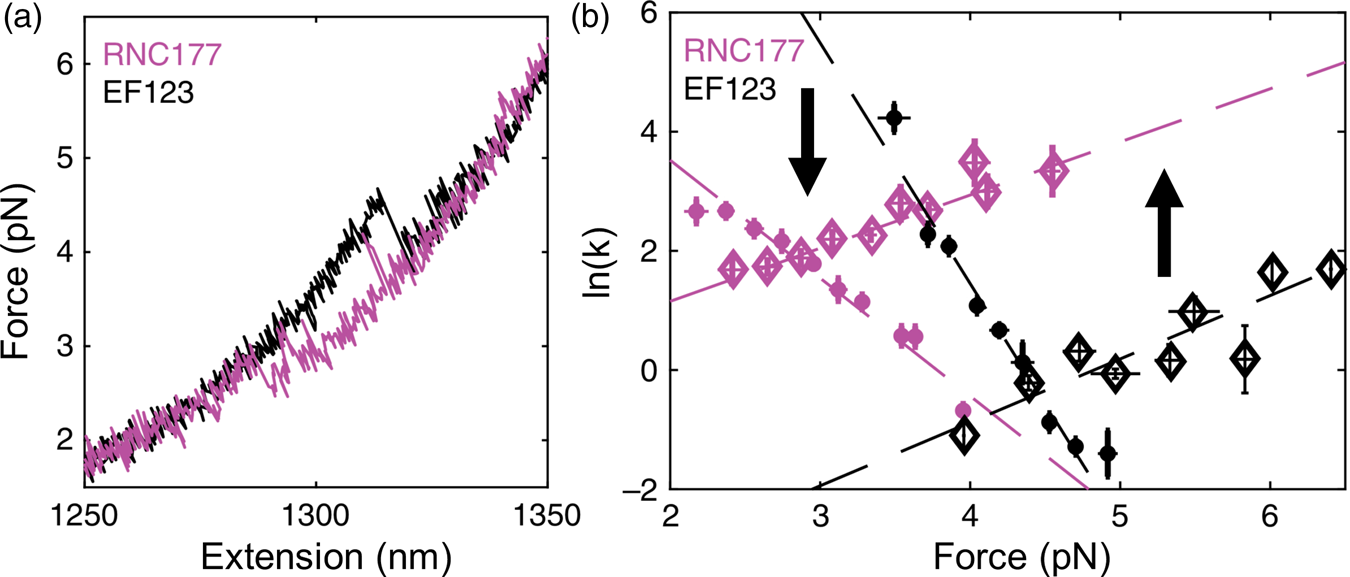
Once again, because the rate of synthesis is very slow relative to the rate of folding, it has been generally assumed that the folding of the growing nascent chain has enough time to equilibrate with its ensemble of accessible conformations after each step of active elongation, and that co-translational protein folding is essentially an equilibrium process. Accordingly, we anticipated that during active synthesis we would expect on average one misfolding event of the nascent EF1 + 2 + 3 per 1.5 s at 4.0 pN. In one of the most difficult single-molecule experiments performed in our laboratory, Lisa managed to use optical tweezers to grab a single calerythrin molecule emerging from the surface of the ribosome and to follow its growth in real-time while simultaneously monitoring its co-translational folding. Much to our surprise, she found that during active translation the misfolded state is only attained after a long delay (τ delay = 63 ± 12 s). In addition, the exponential distribution of the misfolding lifetime suggests that, as the nascent chain is being synthesized, the polypeptide is kept out of equilibrium in the unfolded state (i.e., unable to access the whole ensemble of conformations) until it undergoes a stochastic equilibration step. This trapped unfolded state may involve a set of local interactions with the ribosome surface or with the exit tunnel that were established during its growth in real-time or, alternatively, that may form only in the context of actively elongating ribosome surface dynamics. Note that the unexpected delay of 63 s is long enough to avert misfolding for the remaining duration of translation until the full-synthesized nascent polypeptide emerges, which can then fold through the off-the-ribosome pathway. Lisa's work suggests that the time it takes to prepare the stalled-elongation RNCs for their analysis in the optical tweezers (typically of the order of 15–20 min) is sufficient for them to ‘equilibrate’ and that the measured folding rates of these stalled complexes do not always reflect those of actively translated chains. Moreover, Lisa's work also highlights that co-translational protein folding can be a non-equilibrium process (Alexander et al., Reference Alexander, Goldman, Wee and Bustamante2019).
Other groups have also attempted single-ribosome co-translational folding experiments using in vitro reconstituted translation systems and a dual-trap optical tweezers setup. Specifically, Wruck et al. (Reference Wruck, Katranidis, Nierhaus, Buldt and Hegner2017) monitored the polypeptide synthesis for an unstructured polypeptide and two globular proteins, and they were able to determine possible co-translational folding sites initiated by gradual hydrophobic collapse and correlations between amino acid sequence and nascent chain elongation rate.
Bridging equilibrium and non-equilibrium statistical mechanics: fluctuations theorems
That most proteins show hysteresis when unfolded mechanically meant that we could not get thermodynamic parameters for the process. According to classical thermodynamics, the average work done reversibly on a system to take it from an initial equilibrium state A to a final state B is equal to the change in free energy of the system, i.e., 〈w rev〉≡ ΔG AB. However, the work done to unfold most proteins and RNAs that adopt tertiary structures is often irreversible work. Since the average irreversible work done on the system is the sum of the average reversible work and the average work dissipated in the process, in this case 〈w irrev〉=〈w rev + w diss〉≥ ΔG AB, with the equality holding only when 〈w diss〉= 0. In 1998, I (C.B.) became aware of an article published in 1997 by Christopher Jarzynski, who was working in the theoretical biology division at Los Alamos National Laboratory. In this article, he described his derivation of a remarkable identity (Jarzynski, Reference Jarzynski1997a, Reference Jarzynski1997b). According to this identity, it was possible to extract the free energy of a process carried out irreversibly from the average of the negative Boltzmann exponential of the irreversible work, i.e.:

In other words, Eq. (19) states that the free energy change for a reaction can be determined by averaging negative Boltzmann-weighted work values obtained from repeated irreversible switching of the system. I remember being stunned by this result, and I thought it would be possible perhaps to test it using a single-molecule experiment. While equilibrium statistical mechanics is a well-understood subject that rationalizes the main results of macroscopic thermodynamics from the molecular description of matter, non-equilibrium statistical mechanics remains an area of active research. Surprisingly, the equal sign in Jarzynski's equality represents a bridge between these two realms of statistical physics and, as such, it was truly an outstanding result. At the time when his work appeared, I was about to embark on another move – this time, from Eugene, Oregon to Berkeley, and my students and I were busy packing the laboratory. I remember thinking that once again a move was obliging me to photocopy the article and postpone what could be a crucial experiment. Setting up the laboratory in Berkeley was a tall order. I had appointments in three different departments (Molecular and Cell Biology, Physics and Chemistry) and had equipment and laboratory benches in two of them. This effort kept me busy for a while and for a time I forgot all about Jarzynski's result, until an article by Gerhard Hummer and Attila Szabo (Hummer and Szabo, Reference Hummer and Szabo2001) brought it all back. I approached Jan Liphardt, who had just started his postdoctoral fellowship with Nacho and I, and Sophie Dumont, then a biophysics graduate student, and I suggested them to use an RNA hairpin to test Jarzyinski's equality. We soon agreed that we should use the P5abc RNA domain from the Group I intron in T. thermophila, which unfolds and refolds reversibly under force when stretched and relaxed slowly and does so irreversibly if stretched more rapidly. Jan and Sophie got to work and subjected the RNA hairpin to three different loading rates: 2–5, 34, and 52 pN⋅s−1. As expected, hysteresis in the pulling and relaxation curves was observed only for the intermediate and fast loading rates. Applying Jarzynski's equality to the data obtained with the two fast loading rates yielded values of free energy of unfolding that could be compared with the value derived from the slow loading rate. We found that the equality converged to the value of the free energy obtained from experiments with low loading rates in just under 50 realizations (Liphardt et al., Reference Liphardt, Dumont, Smith, Tinoco and Bustamante2002). Just as important, the experiment revealed very clearly why Jarzynki's relationship works. This is most clearly shown by the plots of the dissipated work values at three different extensions of the molecule (5, 15, and 25 nm) for the three different loading rates (Fig. 20).
Histograms of dissipated work values at x = 5 (a), 15 (b), and 25 nm (c) along the unfolding coordinate. Dissipated work values for a given switching rate were pooled. Blue, 272; green, 119; red, 153 dissipated work values. Solid lines: Gaussian with mean and standard deviation of data. Reprinted with permission from Liphardt et al. (Reference Liphardt, Dumont, Smith, Tinoco and Bustamante2002).
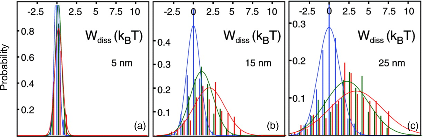
As shown in Fig. 20, the mean and the standard deviation of the dissipated work increase with the loading rate and with the distance along the pulling coordinate (panels A, B, and C). Note also that only when we pull the molecule very slowly the distributions of dissipated work for the different molecular extensions are center around zero (blue curves). The increase of the mean with the loading rate simply indicates that the friction associated with the transition increases with the speed of pulling. Note also that before we start pulling, the molecule is at equilibrium with the thermal bath and therefore samples a Boltzmann distribution of energy states. The faster we pull on the molecule, the less time it has to relax, and an increasingly larger spread (i.e., standard deviation) of the dissipated work distribution is observed, reflecting the spread of those initial energies. Now, the distribution of dissipated work shows that most of the time when we pull the molecule, we end up producing positive dissipation. However, every once in a while a fluctuation in the system occurs such that we end up doing less work that what we would have done if we pulled reversibly the molecule, i.e., w irrev < 〈w rev〉. This is reflected in the fact that all the distributions show a small tail of ‘negative’ dissipated work (smaller than zero). These rare events, however, have a larger statistical weight in the exponential averaging of Eq. (19). Jarzynski's equality asserts that a balance is maintained between the irreversible work trajectories with positive dissipated work values and those with negative ones such that $\langle e^{{-}w_{{\rm diss}}/k_BT}\rangle = 1$ , and the increases in mean and width of the work distributions cancel out, regardless of how quickly a reaction is performed, yielding ΔG independently of the switching rate. Thus, to use the Jarzynski equality, the number of pulling realizations N must be large enough to sample well the rare trajectories that give rise to the negative tail of the distribution. Notice that the cases in which wdiss < 0 are much fewer than those in which wdiss > 0, thus regular averaging of the total work (reversible and dissipated) will always lead to an overestimation of the free energy of a process conducted irreversibly.
The experimental test and confirmation of Jarzynski's result open the path to use it to extract thermodynamic information from mechanical unfolding experiments performed out of equilibrium. Its application reduced to the problem of sampling the rare trajectories responsible for the lower tails in the work distributions. Even at the highest loading rates used in our experiments, the RNA hairpin was never taken more than 3–4 kBT away from equilibrium. Systems that dissipated more work would require a much higher number of realizations. Around the same time, I became aware of a second fluctuation theorem that had been discovered by Gavin Crooks, who was then a graduate student in the laboratory of David Chandler in the Chemistry department at Berkeley. Gavin wished to find a relationship that could quantify the amount of hysteresis when taking a system from an initial to a final state and back. In a remarkably short time after listening to Chris Jarzynski delivering a presentation to Chandler's group, he showed that if P U(W) denotes the probability distribution of the values of the work W performed on the molecule in an infinite number of pulling experiments along the unfolding (U) process, and P R(−W) analogously the probability distribution of the values of the work −W performed by the molecule in the reverse refolding (R) process, then these distributions are related by the following relation (Crooks, Reference Crooks1999):

where ΔG is the corresponding reversible work. Thus, the numerator in the exponent is the amount of work dissipated. For this result, known now as Crooks Fluctuation Theorem (CFT) to be applicable, the unfolding and refolding processes have to be related by time-reversal symmetry. In our experiments, it means that the optical trap used to manipulate the molecule must be moved at the same speeds during unfolding and refolding. Moreover, the molecular transition probed always has to start in an equilibrium state (folded in the unfolding process and denatured or unfolded in the refolding process) and reach a well-defined final state. Also, the CFT does not require the system to reach equilibrium state at the end of the unfolding and refolding processes; only the control parameter (e.g., the position x in time of the trap) must return to its initial value, while the system may continue to equilibrate to a well-defined state allowed by the final value of the control parameter. Equation (20) says that work values greater than ΔG occur most often along the unfolding path while (absolute) work values smaller than ΔG occur most often during the refolding path. Equation (20) also states that when W = ΔG, then P U(W) = P R(W). Therefore, if we plot the unfolding and refolding work distributions obtained experimentally from the pulling (unfolding) and relaxing (refolding) parts of the extension cycle, the point at which they cross will correspond to the free energy of the system. These plots provide a more robust way to obtain the sought-after free energy, making its application desirable for cases involving large dissipations.
A few months prior to our experimental validation of the Jarzynski's equality, I received a letter from Félix Ritort from Spain who wished to join the laboratory as a visiting scholar. Félix was at the time a theorist working in various statistical mechanical aspects of spin glasses. I wrote back telling him that we were interested in fluctuation theorems and their applications to single-molecule force spectroscopy. Félix became immediately interested and soon joined the laboratory. We discussed the idea of using a single-molecule experiment to test experimentally CFT. He and a postdoctoral student in Nacho's laboratory, Delphine Collins, set to test this important theoretical result. Félix and Delphine tested the CFT with two RNA molecules: an interfering (si)RNA that undergoes a transition near-equilibrium and a three-helix junction domain of the 16S RNA from E. coli. In this latter case, they used the CFT to determine the difference in folding free energy for the wild-type RNA and a C.G to G.C mutation (C754G and G587C) of the three-helix junction. They also determined the stabilizing effect of Mg2+ on this molecule. As shown in Fig. 21 the average dissipated work for the unfolding pathway is now much larger – in the range of 20–40 kBT – and the unfolding work distribution shows a large tail and strong deviations from Gaussian behavior. The inset of Fig. 21 shows that a plot of the log ratio of the unfolding to the refolding probabilities versus total work done on the mutant molecule can be fit to a straight line with a slope of 1.06 as expected from Eq. (20). This type of analysis gives a ΔG wt = 154.1 ± 0.4 kBT and ΔG mut = 157.9 ± 0.2 kBT for unfolding the wild-type and mutant types, respectively. After subtracting the handle and RNA entropy loss arising from stretching the unfolded polynucleotide contributions (97 ± 1 kBT) the folding free energies at zero force become ΔG wt(0) = 57 ± 1.5 kBT and ΔG mut(0) = 60.8 ± 1.5 kBT. Free-energy prediction programs such as Mfold and Visual OMP give a ΔΔG(0) = 2 ± 2 kBT at 25 °C and 100 mM NaCl, showing that the CFT furnishes a method precise enough to determine the difference in the folding free energies of RNA molecules differing only by one base pair in 34 base pairs (Collin et al., Reference Collin, Ritort, Jarzynski, Smith, Tinoco and Bustamante2005).
Free-energy recovery and test of the CFT for non-Gaussian work distributions. Plot of unfolding and refolding probabilities on the wildtype (purple) and mutant (orange) 16S RNA three-helix junction without Mg2+. Unfolding (solid lines) and refolding (dashed lines) work distributions. Statistics: wild-type, 900 pulls and two molecules; mutant, 1200 pulls and five molecules. Error bars indicating the range of variability. The crossings between distributions are indicated by black circles. Inset: test of the CFT for the mutant. Reprinted with permission from Collin et al. (Reference Collin, Ritort, Jarzynski, Smith, Tinoco and Bustamante2005).
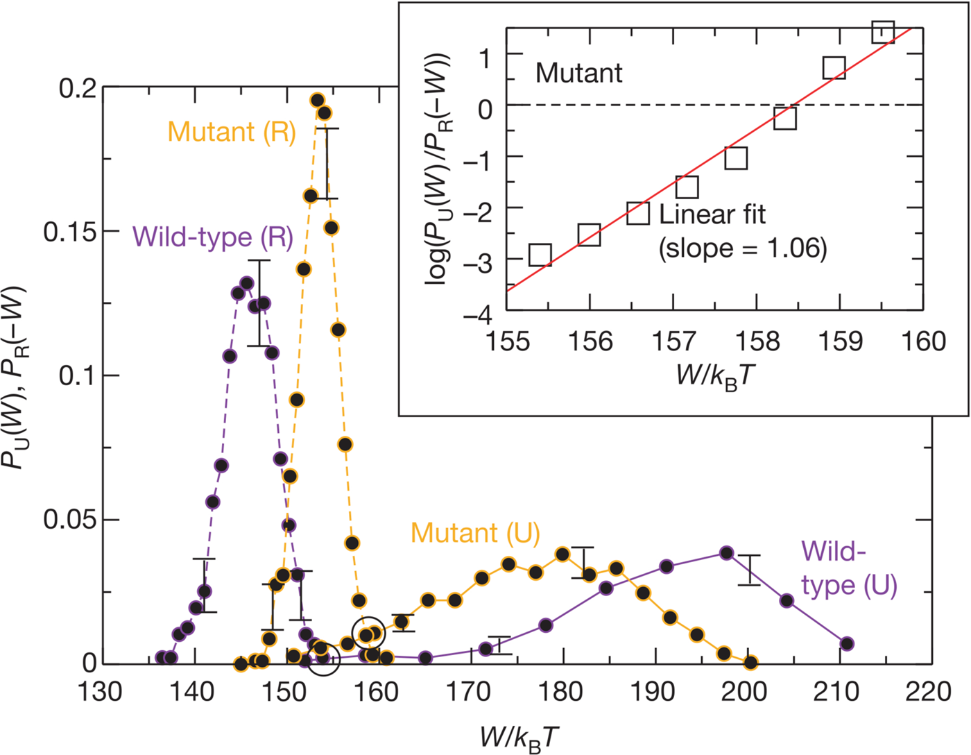
Back in Spain, Félix Ritort and his collaborators introduced a new fluctuation theorem based on the CFT, with which it is possible to calculate the free energy associated with second and higher order binding processes from the irreversible work distributions obtained using single-molecule force spectroscopy. The method requires the unambiguous classification of experimental pulling and relaxation pathways in terms of their initial and final state (folded or unfolded macromolecule and bound or unbound ligand). These authors used this fluctuation theorem to show that it is possible to determine the binding free energy of specific and non-specific macromolecule–ligand interactions and even characterize the cooperative binding between ligand pairs (Camunas-Soler et al., Reference Camunas-Soler, Alemany and Ritort2017).
As illustrated in the previous section ‘Co-translational folding’, complex cellular processes that were thought until now to occur at equilibrium may turn out to involve large relaxation times and happen instead as out-of-equilibrium processes. Accordingly, the discovery of fluctuation theorems and their implementation through single-molecule force spectroscopy experiments are likely to play an increasingly important role in future biophysical studies of those processes. Equally as important, the application of single-molecule force spectroscopy to fluctuation theorems illustrates the power of these methods to investigate non-equilibrium processes in statistical mechanics.
Molecular motors
In an editorial article published in Cell in 1998, Bruce Alberts wrote: ‘The entire cell can be viewed as a factory that contains an elaborate network of interlocking assembly lines, each of which is composed of a set of large protein machines’ (Alberts, Reference Alberts1998). Almost two and a half decades later, this mechanical paradigm about the operation of the cell has now replaced the old one that I (C.B.) was taught back in Peru when I was a biochemistry student. At the time, the cell was viewed as a small bag containing a concentrated solution of macromolecules undergoing second-order reactions. The mechanical paradigm is however not new. In 1666, in his book ‘De Viscerum Structura’, Marcello Malpighi (1628–1694), a professor at the University of Bologna and recognized today as the father of microscopic anatomy, wrote presciently: ‘The operative industry of Nature is so prolific that machines will be eventually found not only unknown to us but also unimaginable by our mind.’ It was a happy coincidence perhaps that at the same time his two great contemporary physicists, Galileo and Newton, were busy perfecting the concepts of force, torque, displacement, mass, acceleration, and energy which became the variables more suited to describe precisely the operation of machines.
The cell milieu is neither isotropic nor homogeneous. Cells have polarity and many of its central processes – from cell motility to internal transport – require directional movement of molecular species through the cytoplasm, across membranes into distinct compartments, and often against chemical gradients. These processes cannot be accomplished by mere diffusion. They require active transport. To perform these directional movements, cells employ tiny machine-like devices that operate as molecular motors, converting chemical energy in the form of bond-hydrolysis or chemical gradients into force and/or torque and displacement. In a more restricted sense, they are enzymes that couple the catalysis of a downhill chemical reaction to the performance of a mechanical task, functioning as energy transducers and converting chemical free energy into mechanical work.
Because force and torque are direct products of these reactions, it follows that externally applied forces and torques can be used to alter their rate, their extent, or even their fate, as well as to learn about their dynamics and mechanisms of operation. Moreover, the variables that are more easily detected by force spectroscopy methods: force, torque, displacement, and time are also the ones of greatest functional value to understand the operation of molecular motors. So, it was natural for researchers interested in studying molecular motors to employ the recently developed methods of single-molecule force spectroscopy.
Transcription studies
In 1995 the laboratories of Steven Block, Jeff Gelles, Robert Landick, and their students published the first force spectroscopy application to the study of DNA-binding molecular motors (Yin et al., Reference Yin, Wang, Svoboda, Landick, Block and Gelles1995). These authors bound an E. coli RNA polymerase non-specifically on the surface of a microscope slide and attached the distal end of the DNA template downstream of the promoter to a bead held in an optical trap. In this way, upon addition of nucleoside triphosphates they could follow the progress of RNA polymerase transcribing along the DNA under tension and working against the force applied by the optical trap (Fig. 22). The experiment yields changes in the distance between the polymerase attached on the glass surface and the downstream end of the DNA template as a function of time, as the enzyme transcribes the DNA. The end-to-end distance of the upstream DNA (see Fig. 22) is force-dependent; therefore, to display the progress of the motor on its track, this distance measured in nm must be converted into the DNA contour length in base pairs. To perform this conversion the authors were able to use the elastic response a DNA molecule to force (Smith et al., Reference Smith, Finzi and Bustamante1992, Reference Smith, Cui and Bustamante1996; Bustamante et al., Reference Bustamante, Marko, Siggia and Smith1994) and the persistence length of the molecule to apply Eq. (1). They found that RNA polymerase could transcribe against forces of around 14 pN. This force is 4–5 times larger than those of cytoskeletal motors. In a follow-up study, these authors characterized the force dependence of the velocity of the motor and found it to be rather insensitive to the applied external load until it decreased sharply at a force between 20 and 25 pN (Wang et al., Reference Wang, Schnitzer, Yin, Landick, Gelles and Block1998). Using an Arrhenius dependence to describe the effect of the force on the velocity of the motor (Eq. (16)), they found that the corresponding distance to the transition state leading to the stall of the motor was between 5 and 10 bp. The authors noted that such large distance was unphysical and suggested that it could be rationalized if under applied force the molecule moved backwards. This observation was consistent with RNA polymerase backtracking, a built-in editing mechanism of the enzyme previously discovered using bulk studies (Komissarova and Kashlev, Reference Komissarova and Kashlev1997b). A few years later, Steven Block and collaborators were able to visualize the backtracking of the enzyme at near-base pair resolution (Shaevitz et al., Reference Shaevitz, Abbondanzieri, Landick and Block2003).
A cartoon illustrating (not to scale) the configuration during subsequent transcriptional elongation. The trap center is located on the optical axis but slightly above the narrow waist of the focused laser beam. The polymerase has proceeded for some distance along the DNA, shortening the segment between the bead and the polymerase. The bead is pulled away from the trap center (arrow), increasing the restoring force of the trap. Reprinted with permission from Bustamante et al. (Reference Bustamante, Chemla, Liu and Wang2021).
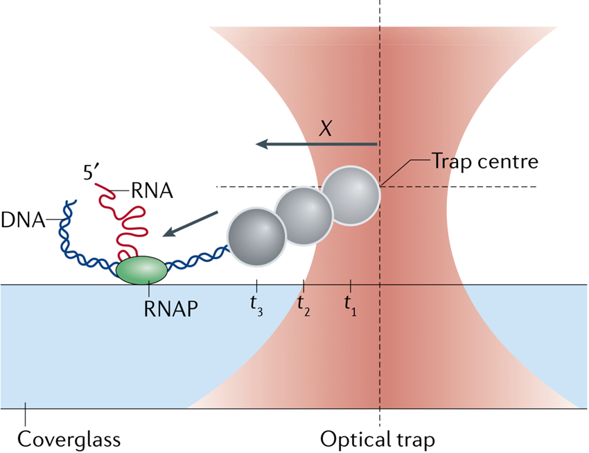
Around this time, two of my graduate students, John Davenport and Gijs Wuite, began to investigate the dynamics of RNA polymerase during transcription using a combined optical tweezers-hydrodynamic flow instrument design. They found significant dispersion in the enzyme's transcription rate, and that this dispersion could be both static (variation among molecules) and dynamic (variation within a molecule). Moreover, they found that the enzyme had high propensity to pause in certain locations along the template. They showed that the probability of pausing (pausing efficiency) was inversely correlated with the rate of transcription of the enzyme prior to entering the pause, supporting the idea that elongation and pausing compete kinetically (Erie et al., Reference Erie, Hajiseyedjavadi, Young and Von Hippel1993; Landick, Reference Landick1999). This observation is consistent with earlier results showing that pauses correspond to states off the main elongation pathway (Erie et al., Reference Erie, Hajiseyedjavadi, Young and Von Hippel1993; Landick, Reference Landick1999). John's and Gijs's results were corroborated by data obtained by Nancy Forde, a postdoctoral fellow. Nancy used optical tweezers to characterize the effect of assisting versus opposing force on E. coli RNAP and found that the former does not alter the translocation rate but reduces the pausing and permanent arrest efficiency of the enzyme. Moreover, arrested molecules cannot be rescued by force, suggesting that arrest involves enzyme backtracking along the DNA followed by a conformational change of the ternary complex (RNA polymerase, DNA, and transcript), which renders this molecular motor permanently inactive (Forde et al., Reference Forde, Izhaky, Woodcock, Wuite and Bustamante2002).
Next, we wished to investigate how the eukaryotic RNA polymerase (RNAP II) transcribes when it encounters a nucleosome. Nucleosomes represent barriers to transcription whose epigenetic modification constitutes an important mechanism of control of gene expression. Before accomplishing this task, however, we had to characterize first the dynamics of RNAP II from yeast while transcribing bare DNA. Eric Galburt and Stephan Grill, at the time two postdoctoral associates in the laboratory, used a dual-trap optical tweezers to perform this characterization. Erick and Stefan found that the response of RNAP II to an opposing force is entirely determined by enzyme backtracking (Roeder, Reference Roeder1996; Nudler et al., Reference Nudler, Mustaev, Lukhtanov and Goldfarb1997; Komissarova and Kashlev, Reference Komissarova and Kashlev1997a, Reference Komissarova and Kashlev1997b; Kireeva et al., Reference Kireeva, Hancock, Cremona, Walter, Studitsky and Kashlev2005). To our surprise they found that RNAP II molecules ceased to transcribe and were unable to recover from backtracks at a force ~7.5 pN, only a third of the stall force determined for the E. coli RNAP (Wang et al., Reference Wang, Schnitzer, Yin, Landick, Gelles and Block1998; Davenport et al., Reference Davenport, Wuite, Landick and Bustamante2000). We suspected that 7.5 pN represented only an ‘operational’ stall force due to the tendency of the molecule to backtrack and that the enzyme could transcribe against higher forces. To illustrate the concept of an operational force, I used the following analogy with my students: Imagine that someone is threateningly coming towards you, and you need to stop him. You will measure two very different ‘stall’ forces of the individual if you grab the person by the shoulders than if you just put your finger on one of his eyes as he advances towards you. The latter is only an ‘operational’ stall force of that individual. To test the hypothesis of an operational force in RNAP II, we decided to perform ‘force jump’ experiments during active enzyme translocation, wherein the force exerted on the polymerase was suddenly increased by displacing one of the two traps. We then restored the original position of the trap (i.e., lowered the force) after 1 s and determined the velocity of the enzyme during the jump. For 50% of the force-jump experiments, we observed RNAP II transcription at 14–20 pN, and for 17% between 20 and 25 pN. No enzymes were seen to transcribe over 25 pN. This is the result one would expect if the rate of forward translocation is larger than the rate of entering a backtracking trajectory. Namely, when we increase the force opposing RNAP II, if the enzyme is still able to transcribe against a higher force, it will continue transcribing for a while at that force before backtracking.
Furthermore, we found that the distribution of backtrack pause duration before transcription restarts follows a t −3/2 power-law. Such dependence is to be expected if RNAP II during backtracking diffuses back and forth on the template DNA in discrete base-pair steps – before the active site of the enzyme re-engages the 3′-end of the transcript and is able to resume transcription. Soon after, Stephan and Eric were able to show analytically the t −3/2 power law was to be expected from a diffusion model of the enzyme during backtracking (Depken et al., Reference Depken, Galburt and Grill2009). This power-law dependence also suggests that backtracking is the dominant mechanism of pausing for RNAP II. Importantly, Eric and Stefan showed that the backtracked RNAP II can be rescued by the transcription factor TFIIS added in trans and that in the presence of this factor the enzyme can proceed to transcribe against a force up to 17 pN. This result reflects how transcription regulation can be achieved by factors that modify the mechanical performance of the enzyme (Galburt et al., Reference Galburt, Grill, Wiedmann, Lubkowska, Choy, Nogales, Kashlev and Bustamante2007).
Having characterized the dynamics of the eukaryotic RNAP II on bare DNA, we were then in the position to find out how the enzyme behaves upon encountering a nucleosome. It was already surprising that RNAP II, an enzyme that must transcribe through the barrier imposed by nucleosomes is three times weaker than its prokaryotic counterpart. Because nothing in biology is fortuitous, it is possible that a weaker version of the enzyme could be an evolutionary strategy to make its progress through chromatin a better target of regulation by cis- or trans-acting factors. Motivated by these ideas two graduate students, Courtney Hodges and Lacra Bintu, took upon themselves to determine how the enzyme transcribes nucleosomal DNA. Figure 23a shows the geometry of their experiment, where an artificial bubble initiation system (Komissarova et al., Reference Komissarova, Kireeva, Becker, Sidorenkov and Kashlev2003) was adapted to follow the RNAP II transcription. The nucleosome is bound to a 601 nucleosomal positioning sequence (NPS) to insure its proper position on the DNA template (Lowary and Widom, Reference Lowary and Widom1998). The molecular trajectories of individual polymerases showed that, in the absence of other factors, the enzymes alone spend a long time crossing the nucleosomal barrier, displaying long pauses, where the crossing time depends on the ionic strength of the buffer medium (Fig. 23b). Based on their results, Courtney and Lacra formulated a model according to which RNAP II is not mechanically strong enough to peel the DNA from the surface of the nucleosome. Instead, their data indicated that the nucleosome functions as a fluctuating barrier, with the DNA constantly wrapping and unwrapping from the histone core in front of the enzyme, which exploits the periods in which the DNA transiently unwraps to advance on the template, thus acting as a rectifier of those fluctuations (Hodges et al., Reference Hodges, Bintu, Lubkowska, Kashlev and Bustamante2009).
Transcription through a nucleosome. (a) Geometry for the dual-trap optical tweezers experiments. (b) Representative trajectories of individual transcribing polymerases with or without the nucleosome at different ionic strengths. The shaded region represents the NPS. Reprinted with permission from Hodges et al. (Reference Hodges, Bintu, Lubkowska, Kashlev and Bustamante2009).

In a subsequent paper, Lacra Bintu, together with graduate student Manchuta Dangkulwanich and postdoctoral associate Toyotaka Ishibashi, used the same experimental design as in Fig. 23 to obtain the first topographic characterization of the barrier (Bintu et al., Reference Bintu, Ishibashi, Dangkulwanich, Wu, Lubkowska, Kashlev and Bustamante2012). By mapping the residence time of the enzyme at different points into the nucleosome, they were able to determine an entry, a central, and an exit region of the barrier (Fig. 24).
Histone tails affect RNA polymerase II pausing in the nucleosome entry region. Pause density as a function the position of the active center of Pol II on the template for tailless (panel A) and acetylated (panel B) nucleosomes. The nucleosome entry/exit regions are shaded yellow, and the central region is shaded gray. Error bars represent s.e.m. Reprinted with permission from Bintu et al. (Reference Bintu, Ishibashi, Dangkulwanich, Wu, Lubkowska, Kashlev and Bustamante2012).
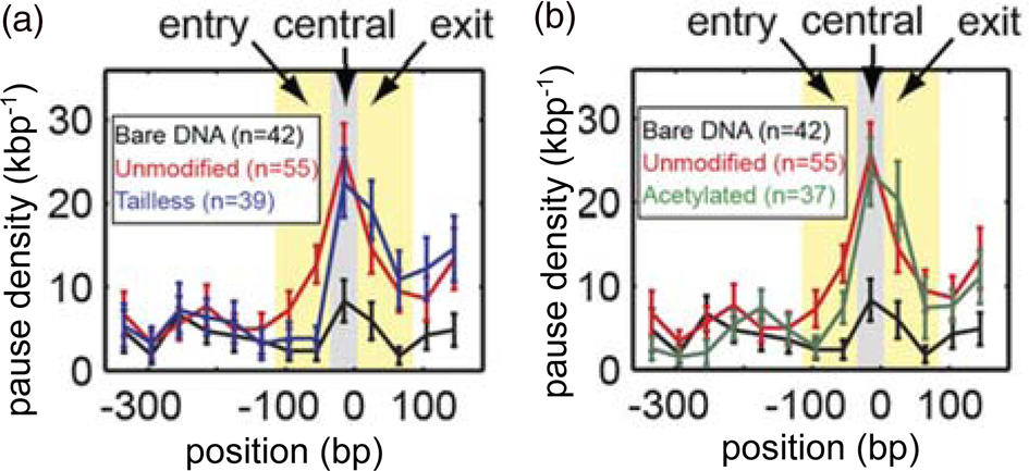
They found that removal of the histone tails favors the progress of the enzyme into the entry region (Fig. 24a). Furthermore, histone mutations that target the histone-DNA contacts near the nucleosome dyad abolish the barrier to transcription in the central region by decreasing the local DNA wrapping rate, while acetylation of the histone tails weakens only slightly the entry region.
These studies allowed us next to attempt a high-resolution, high-accuracy mapping of the transcription barrier. Three postdoctoral fellows, Zhijie Chen, Ronen Gabizon, and Cesar Diaz, together with graduate student Antony Lee, collaborated in this tour-de-force project. The geometry of the experiment is illustrated in Fig. 25a, where a dual trap ultra-high-resolution instrument is used to tether RNAP II via a DNA handle linked to a bead that is kept in one of the optical traps, and the DNA template upstream of the polymerase is tethered to a bead held in the other trap. Downstream from the polymerase we engineered an 8-tandem repeat of a sequence that has been shown to efficiently pause the polymerase, followed by a 601 NPS to which a nucleosome is stably bound. The eight strong pauses of the enzyme, ahead of its encounter with the nucleosome, allowed them to precisely align the molecular trajectories of different polymerases relative to each other so that the data could be averaged together. The improved accuracy, together with the high spatial resolution and minimal drift of the instrument, yielded topographic maps of the barrier with single base pair resolution and accuracy for canonical nucleosomes, for nucleosomes harboring the histone variant H2A.Z, and for nucleosomes with monoubiquitinated H2B (uH2B) (Fig. 25b). RNAP II crossing dynamics are complex, displaying pauses at specific loci, backtracking, and nucleosome hopping between different wrapped states. While H2A.Z widens the barrier, uH2B increases the barrier height, and both modifications greatly lengthen RNAP II crossing time. From the dwell times of RNAP II at each nucleosomal position we were able to extract the energetics of the barrier crossing. The orthogonal barrier modifications introduced by H2A.Z and uH2B, and their effects on RNAP II dynamics, help to rationalize their observed enrichment in +1 nucleosomes and suggest a mechanism for selective control of gene expression (Chen et al., Reference Chen, Gabizon, Brown, Lee, Song, Diaz-Celis, Kaplan, Koslover, Yao and Bustamante2019).
A ‘molecular ruler’ gauges the positions of an elongating Pol II with near-basepair accuracy. (a) Experimental design of an improved single-molecule nucleosomal transcription assay. A single biotinylated Pol II (purple) is tethered between two optical traps. Transcription is measured as increases in distance between the two beads at 10 pN constant force. Inset: composition of the tethered molecule, which is constructed by ligating Pol II stalled complex (cyan), the molecular ruler (green), NPS DNA (or nucleosome, yellow + gray), and a short inter-strand crosslinked DNA at the end (red; so as to stall Pol II). The ‘molecular ruler’ consists of eight tandem repeats of a 64 bp DNA (green), each harboring a single sequence-encoded pause site. (b) A representative trace of a single Pol II transcribing through a Xenopus WT nucleosome. The black dashed lines indicate NPS entry, dyad, and exit, respectively. Inset: Zoom-in of the boxed region, highlighting the repeating pause patterns within the ‘molecular ruler’. The gray dashed lines are the predicted pause sites, whereas the short green lines mark the actual pauses of Pol II. (c) Zoom-in of Pol II dynamics within the NPS region of panel B. The right y-axis (in bp) is offset to the beginning of the NPS. The left y-axis shows regions preceding the dyad as superhelical locations (SHL) in red. Black arrows indicate events of backtracking, pausing, productive elongation, and hopping. Regions corresponding to Pol II located at SHL (−5) and SHL(−1) are indicated with green and cyan dashed lines, with the corresponding Pol II-nucleosome complex structures shown on top (PDB 6A5P for PolII-SHL(−5), 6A5T for PolII-SHL(−1)). Pol II, histones, template DNA, non-template DNA are colored in gray, green, red, and blue, respectively. (d) Transcriptional maps of the nucleosome reveal that H2A.Z enhances the width and uH2B the height of the barrier. Median residence time histograms of Pol II transcription through bare NPS DNA (black), Xenopus WT (xWT, orange), human WT (hWT, red), H2A.Z (blue), and uH2B (green) nucleosomes. Bar width: 1 bp; major peak positions are labeled (in bp) above the corresponding peaks. NPS entry, dyad, and exit are marked with blue dashed lines. The top x-axis (red) indicates positions of the first half of nucleosome expressed as SHL. Polar plots on the right project the residence time histogram onto the surface of nucleosomal DNA, thus representing the corresponding transcriptional maps of the nucleosome. Reprinted with permission from Chen et al. (Reference Chen, Gabizon, Brown, Lee, Song, Diaz-Celis, Kaplan, Koslover, Yao and Bustamante2019).
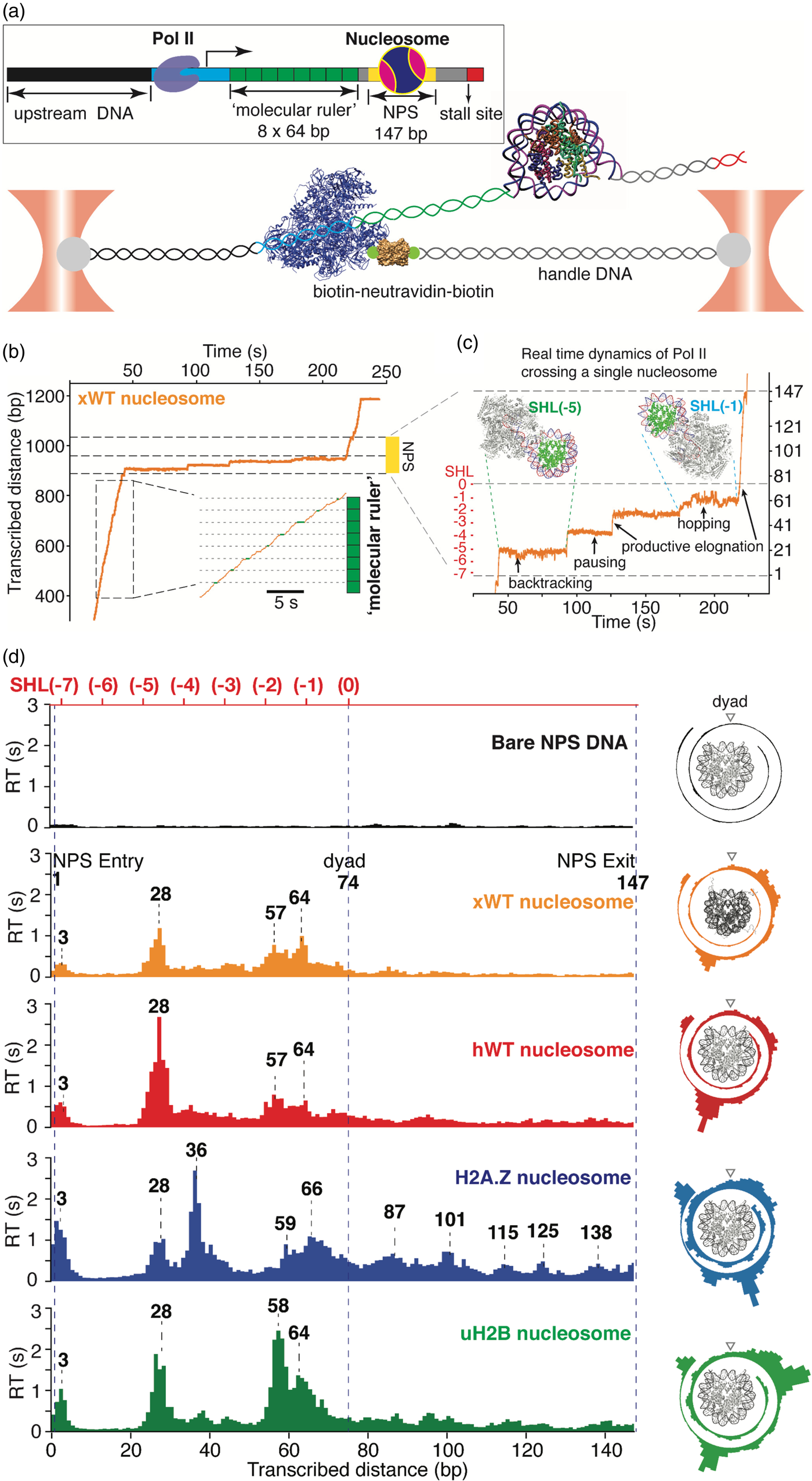
DNA polymerase
Because of its high processivity, RNA polymerase can be directly tethered in single-molecule experiments to follow the enzyme's progression on the DNA template. This direct tethering approach, however, is not applicable for studies of distributive enzymes such as DNA polymerases that bind for a short time to ssDNA replicate a few tens of bases into dsDNA and detach soon after. Therefore, to study T7 DNA polymerase, we decided to develop an assay that took advantage of the difference in the elastic response of dsDNA and ssDNA that we had previously characterized (Cluzel et al., Reference Cluzel, Lebrun, Heller, Lavery, Viovy, Chatenay and Caron1996; Smith et al., Reference Smith, Cui and Bustamante1996) (see section ‘The entropic elasticity regime’). The different elasticity can be clearly seen from the force-extension curves of dsDNA and ssDNA with the same number of base pairs and nucleotides, respectively, as shown in Fig. 26b. Hence, if we tether a ssDNA molecule between two beads and hold it at some constant value of the force above 7 pN, its conversion into dsDNA – upon DNA replication by the polymerase – will necessarily be accompanied by a decrease in its end-to-end distance, which furnishes an experimental readout of the enzyme activity. Conversely, holding the tether at a force below 7 pN, the observed end-to-end distance will increase as the polymerase converts ssDNA into dsDNA. The geometry of such experiment is shown in Fig. 26a.
(a) A 10 416 bp plasmid DNA fragment was attached between two beads, one held on the tip of a glass pipette, the other in an optical trap. ssDNA was obtained by using the force-induced exonuclease activity of T7 DNA polymerase (T7 DNAp) to remove any desired length of the non-template strand. (b) Force–extension data for dsDNA and ssDNA (black dotted lines), compared with the wormlike chain model (solid red lines) using ssDNA and dsDNA persistence lengths of 0.75 nm and 53 nm respectively. (c) Replication of an ssDNA template under 20 pN tension using 8 nM T7 DNAp. Upper red curve: conversion to dsDNA plotted as fraction of ssDNA left in the template versus time. Lower black curve: polymerization rate obtained by differentiating upper curve after smoothing it with a moving-average filter (24 data points) to reduce Brownian noise. Reprinted with permission from Wuite et al. (Reference Wuite, Smith, Young, Keller and Bustamante2000).
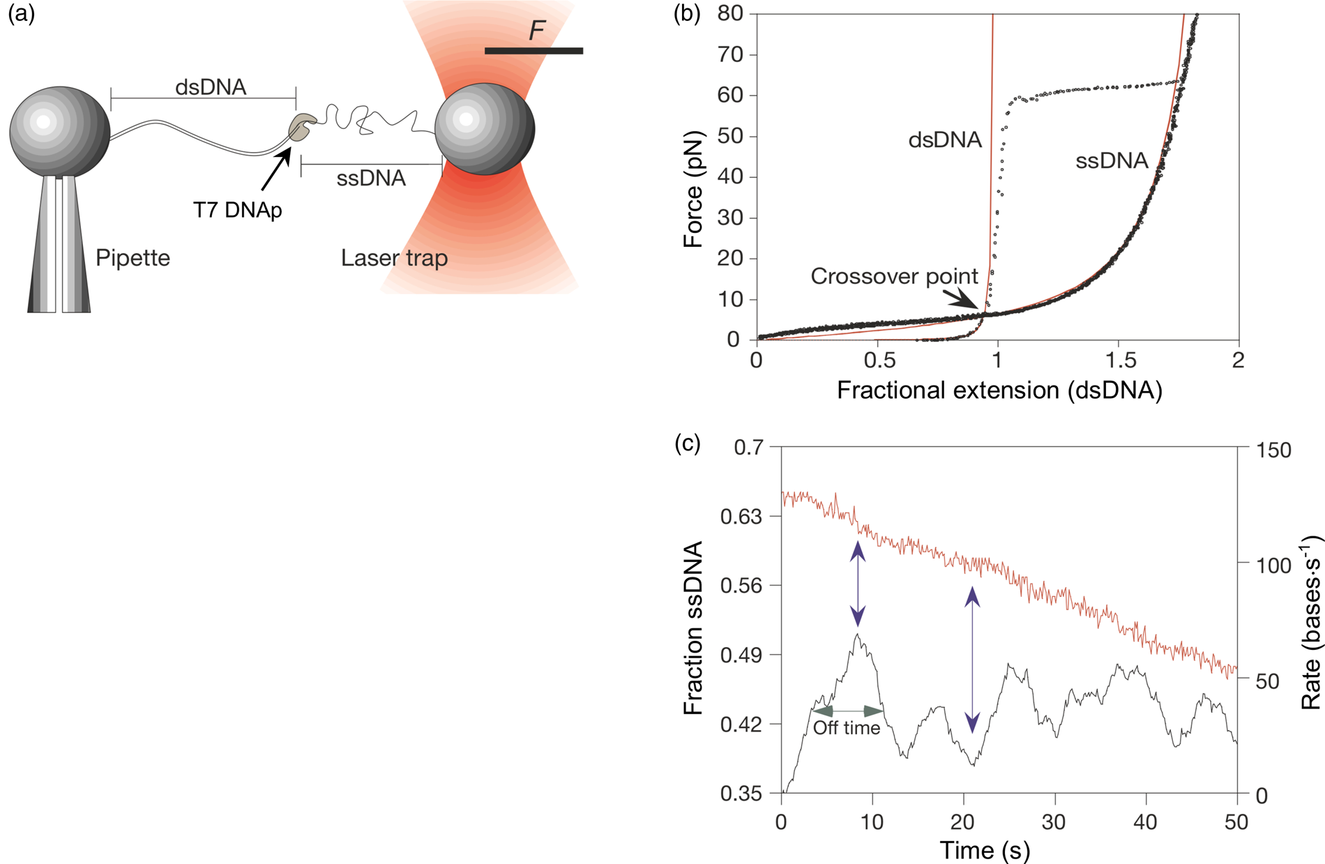
Accordingly, the progress of a DNA polymerase can be followed by the number of ssDNA nucleotides remaining in the tether at time t, given by:

where xmeas(F, t) is the experimental end-to-end distance of the molecule at force F and at time t; x ds,ss(F) are the end-to-end distances of fully double- or single-stranded DNA molecule at that force, and Ntot is the total number of bases in the ssDNA template. Figure 26c depicts the fraction of ssDNA remaining after time t (upper line in red). The time derivative of the fraction of ssDNA remaining at time t yields the instantaneous polymerization rate (lower line in black), where peaks corresponding to burst of enzyme activity reflect periods during which a polymerase was engaged in DNA replication and valleys correspond to periods in which no polymerase is bound to the 3′ end of the growing chain. Repeating the experiments at different forces, we were able to show that the rate of polymerization is slightly higher on an ssDNA template under tension below 7 pN and decreases monotonically when the tension applied to the template is above 7 pN until about 30–35 pN.
Surprisingly, for tensions above 35 pN we observed a lengthening of the tether, corresponding to the stimulation of the exonuclease activity of the enzyme which converts dsDNA into ssDNA. Apparently, the tension applied to the tether above 35 pN induces a structural deformation of the dsDNA base pairing at the active site, which triggers the exonuclease editing activity of the enzyme (Fig. 27) (Wuite et al., Reference Wuite, Smith, Young, Keller and Bustamante2000). Similar tension-induced exonuclease activity was also found by Borja Ibarra, a postdoctoral fellow, with the DNA polymerase from bacteriophage phi29, which unlike the T7 version is able to polymerize processively along the template DNA and stalls at a slightly higher force of ~37 pN. When the tension on the DNA substrate exceeds ~46 pN, the actively replicating phi29 DNA polymerase first comes to a pause, which is an obligatory intermediate state before it switches to the editing mode and begins to degrade processively the primer strand. Furthermore, the processivity of its exonuclease activity increases with force, hence indicating that tension not only triggers the intramolecular transfer of the primer strand from the polymerization to the exonuclease active sites within the phi29 DNA polymerase but also stabilizes the editing conformation of the enzyme. Importantly, when the high tension is dropped below ~37 pN, the processive exonucleolysis comes to a halt, and within a few seconds (~3.2 s) the polymerase resumes DNA replication. Therefore, by resolving changes in DNA extension – namely, the conversion between ssDNA and dsDNA – we were able to identify kinetics intermediates of DNA polymerase, whose pause states may serve as an off-pathway fidelity checkpoint for its proofreading operation (Ibarra et al., Reference Ibarra, Chemla, Plyasunov, Smith, Lazaro, Salas and Bustamante2009).
Force dependence of 3′→5′ exonuclease reaction. Diamonds represent average rates for 49 exonuclease bursts measured at 9 different forces. Traces represent three lines fitted through successions of exonucleolysis burst heights (triangles) initiated at high tensions on DNAs kept at constant end-to-end distances. Digestion lowers the tension on the DNA until the fast exonucleolysis stops. The upper limit for these experiments is determined by the overstretching force of dsDNA, 65 pN. Near the stalling force for polymerization, a competition was occasionally observed between exonucleolysis and polymerization which caused the template tension to bounce up and down every few seconds. Reprinted with permission from Wuite et al. (Reference Wuite, Smith, Young, Keller and Bustamante2000).
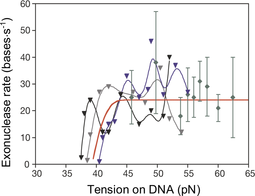
Wang and collaborators used the unzipping DNA geometry (see section ‘Mechanical melting of DNA’) to show that the DNA polymerase from bacterial phage T7 works in conjunction with its helicase and can directly replicate through a DNA lesion instead of dissociating from the template (Sun et al., Reference Sun, Pandey, Inman, Yang, Kashlev, Patel and Wang2015).
DNA packaging motor
Besides RNA and DNA polymerases, we and many other groups had become interested in understanding the molecular mechanisms underlying the operation of P-loop NTPases (Burroughs et al., Reference Burroughs, Iyer and Aravind2007). In particular, the ASCE (i.e., additional strand catalytic E) division from this group of enzymes represents a structurally homologous yet functionally diverse set of proteins that often form multimeric rings and that are involved in various essential tasks in the cell (Liu et al., Reference Liu, Chistol and Bustamante2014a). The first member of the ASCE family that we studied was the DNA packaging motor of the small icosahedral bacteriophage phi29, whose host is Bacillus subtilis. In 1997, still in Eugene, Oregon, Steve Smith and I (C.B.) met with Dwight Anderson, Paul Jardine, and Shelley Grimes from the University of Minnesota to discuss the possibility of studying this motor using our force spectroscopy approach. The following year, having just unpacked our instruments after the move to Berkeley, we started to develop a single-molecule DNA packaging assay for this motor. Two physicists, Doug Smith and Sander Tans, had joined my laboratory as postdoctoral associates, and they immediately set to work on this system.
The phi29 DNA packaging motor is made up of three co-axial rings: a dodecamer that binds to the opening at the base of the viral capsid, a pentameric ring made of RNA, and a pentameric ring of protein gp16, which is the ATPase (Mao et al., Reference Mao, Saha, Reyes-Aldrete, Sherman, Woodson, Atz, Grimes, Jardine and Morais2016). The experimental design by Doug and Sander is shown in Fig. 28. A single capsid head of a phi29 virus that has begun to package its genome is attached to a bead kept by suction atop a micropipette, and the distal end of the DNA is connected to a bead held in an optical trap (indicated by the tick marks). As packaging progressed, they could either move the micropipette closer to the trapped bead to maintain a constant force load on the motor, or hold the distance between the trap and the bead on the pipette constant. In the latter case, as the motor packages the DNA it pulls the bead from the center of the trap, thereby increasing the force against which the motor must operate. This constant position or ‘passive force’ experiment permits us to determine how the motor's velocity responds to increasing mechanical load. Once again, we could convert the end-to-end distance of the DNA tether into number of base pairs using the elastic behavior of dsDNA that we had previously characterized (see section ‘The entropic elasticity regime’). Using the constant force mode of the instrument, we found that the motor velocity at the beginning of packaging was ~100 bp s−1 and that it starts to decrease when approximately 50% of the DNA has been internalized (Fig. 29a and b).
Experimental set-up at the start of a DNA packaging measurement (left), constant force feedback mode (middle), and no feedback mode (right) measurements. A single phi29 packaging complex is tethered between two beads. Optical tweezers are used to trap one bead and measure the forces acting on it, while the other bead is held by a micropipette. Such molecule attachments break in one discrete step as the force is increased, indicating that only one DNA molecule carries the load. Reprinted with permission from Smith et al. (Reference Smith, Tans, Smith, Grimes, Anderson and Bustamante2001).
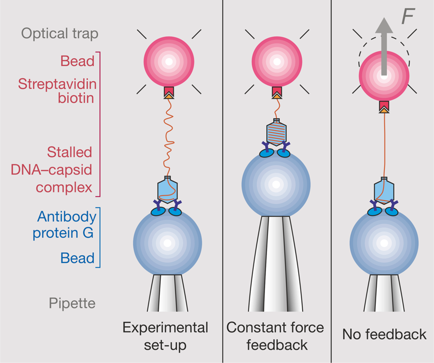
(a) DNA tether length versus time for four different phi29 packaging complexes under a constant force of ~5 pN using a 34.4 kb phi29-λ DNA construct. Inset: increased detail of regions, indicated by arrows, showing pauses during packaging. Black solid lines are a 100-point average of the raw data (gray and cyan). (b) Packaging rate versus the amount of DNA packaged, relative to the original 19.3-kb phi29 genome. Rates were obtained by linear fitting in a 1.5-s sliding window. The red line is an average of eight such measurements. Large pauses (velocity drops >30 bp s–1 below local average) were removed. The red line was smoothed using a 200-nm sliding window. (c) Stall force measured for 65 individual complexes indicates an average stall force of ~57 pN. Stall force refers to the total force (external force plus, in the case of two-thirds of the genome being packaged, the inferred internal force of 14 pN), which is needed to stop further packaging. Reprinted with permission from Smith et al. (Reference Smith, Tans, Smith, Grimes, Anderson and Bustamante2001).

Using the constant position mode, Doug and Sander also showed that the motor velocity was sensitive to the applied external force (Fig. 30a), indicating that the translocation step in the mechanochemical cycle of the motor was rate-limiting under saturating [ATP]. They also found that the average stall force of the motor was about 60 pN (Fig. 29c), reaching in some cases 70 pN, i.e., 15–20 times that of myosin. In addition, they made a very subtle observation: they noticed that the force–velocity relation for packaging when the capsid is two-thirds filled with DNA (solid blue) is very similar to that obtained when the capsid is only one-third filled (red) but appears shifted relative to the latter by ~15 pN (dashed blue; Fig. 30b). This observation implies that as the motor fills the viral capsid, an internal pressure builds up and opposes packaging, thus giving rise to the shift towards lower mechanical loads. From the force–velocity curves obtained at different filling levels, they were able to determine the internal pressure accumulated inside the capsid as the viral genome was packaged. As seen in Fig. 30c, and consistent with the dependence of the packaging rate on the percent genome packaged (Fig. 30b), this internal force due to pressure buildup emerges when ~50% of the genome is packaged and grows steadily as the capsid fills up. Later studies by other groups (Evilevitch et al., Reference Evilevitch, Castelnovo, Knobler and Gelbart2004; Philips et al., Reference Philips, Kondev, Theriot and Garcia2012) confirmed the buildup of an internal pressure, which nearing the end of packaging we estimated to be ~3 MPa or 30 atmospheres, i.e., six times the pressure inside a bottle of a champagne! This result begs the question of why a powerful motor has evolved to work against such large internal pressure if the same task could have been accomplished by a much weaker machine with a capsid twice as large! The answer to this question reveals the mechanical nature – often ignored until the advent of single-molecule force spectroscopy – of many biological processes. The phage not only must package its genome in about three and a half minutes to ensure its reproductive viability, but it also has to solve the problem of how to introduce its DNA into the host in the next cycle of infection. The solution to the problem is indeed mechanical. What the phage does is to convert the free energy from the hydrolysis of ATP into potential mechanical energy and store it inside the capsid in the form of a loaded spring (the packaged DNA). At the end of the infection cycle when packaging is completed, the RNA and gp16 rings detach from the capsid and are replaced by the phage tail. Soon after, the host cell lyses and releases the newly formed viruses. Each of these viruses can then bind to their receptors on the surface of a new host cell to initiate a new cycle of infection. Here is when they can use the potential energy stored in the capsid and convert it into mechanical kinetic energy, effectively injecting their DNA into the new host under pressure. These results were published in 2001 (Smith et al., Reference Smith, Tans, Smith, Grimes, Anderson and Bustamante2001).
(a) Packaging rates as a function of force, where three complexes are shown as examples (black, red, and blue lines, respectively). These lines are obtained by editing out large pauses (asterisks indicate where velocity drops >30 bp s–1 below local average in the raw data, gray line) and smoothing (50-point sliding window). These long pauses were removed so as not to perturb the general trend of the force–velocity (F-v) behavior. (b) External force against velocity curves when about one-third (red line) and about two-thirds (blue line) of the genome is packaged. Curves were obtained from averaging 14 and 8 individual traces, respectively. If, in the case of two-thirds of the genome being packaged, an additional 14 pN (light blue arrow) of internal force were acting on the motor, the dashed blue line would show the expected behavior. The red line and the dashed blue lines would then represent the inherent (total) F-v curve for the motor. (c) Internal force against percentage genome packaged. This plot is obtained by relating the packaging rate, as obtained from the rate against percentage of genome packaged curve (Fig. 29b), to the total force required to produce the same packaging rate, as given by the rate against force curve (see panel B, average of red and dashed blue lines). The internal force is obtained by subtracting from the total force the 5 pN of external constant force that is present in these experiments. Reprinted with permission from Smith et al. (Reference Smith, Tans, Smith, Grimes, Anderson and Bustamante2001).
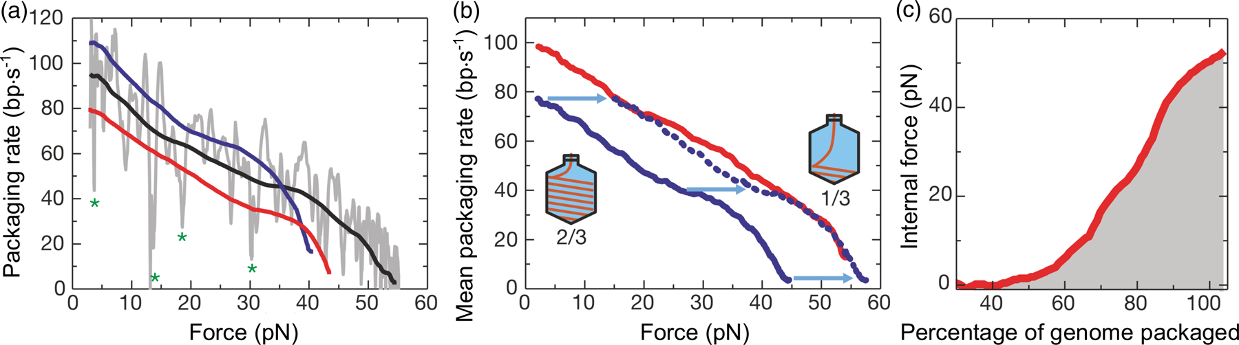
As an independent investigator at the University of California at San Diego, Doug Smith and collaborators showed that it was possible to monitor the initiation phase of the packaging process by directly bringing the end of a DNA molecule attached to a bead in an optical trap, in contact with phage proheads bound to the surface of another bead in the second laser trap (Rickgauer et al., Reference Rickgauer, Fuller, Grimes, Jardine, Anderson and Smith2008). An interesting question is whether the confinement of DNA during packaging occurs at equilibrium, proceeding quasi-statically, or if it is essentially a non-equilibrium process. Doug and collaborators investigated this question using an assay in which packaging was allowed to reach 75% prohead filling. At this point the motor was stalled with non-hydrolyzable ATP. They found that when packaging was restarted by addition of ATP after an imposed waiting time, the motor resumed its operation at a higher velocity, indicating that during the initial packaging period the DNA was in a non-equilibrium state that had been allowed to relax during the stall period (Berndsen et al., Reference Berndsen, Keller, Grimes, Jardine and Smith2014).
In 2000 my colleague David Keller and I had developed a theory of molecular motors that describes the motor's operation as a diffusion process over a potential energy surface, where one dimension represents a chemical reaction coordinate and the other describes the spatial displacement of the motor (Fig. 31) (Keller and Bustamante, Reference Keller and Bustamante2000). The coupling between these two coordinates arises from the shape of the surface, and motor velocities and forces result from diffusion currents on this surface. From this microscopic description we derived an equivalent kinetic mechanism in which some of the rate constants depend on externally applied forces. In this description, assisting and opposing forces correspond to tilting of the potential energy surface around the chemical axis; similarly, an increase or decrease of [ATP] corresponds to tilting the surface around the mechanical axis. This formulation allowed us to classify the different types of motors based on their kinetic schemes according to where the actual mechanical step (i.e., the one sensitive to the application of force and usually coincident with translocation) occurred relative to the binding of the fuel (ATP or GTP) and the release of the products upon hydrolysis (ADP or GDP, and inorganic phosphate, Pi). The classes of motor were defined by whether the actual force generation coincides with the process of nucleotide binding, nucleotide hydrolysis, or the release of products. We were able to obtain general expressions for motor velocity versus loading force for any member of each class. We further showed that in some cases, Lineweaver–Burk plots of 1/velocity versus 1/concentration of fuel in which the force acts as an inhibitor of the motor permit the identification of the class to which the motor belongs and where in the motor kinetic scheme force is generated and transloction occurs. In other words, the force dependence of V max, K M or V max/K M can be used to discriminate among the different classes. By then a new postdoctoral associate Yann Chemla, a physicist by training, had joined the group, and in collaboration with a biophysics graduate student, K. Aathavan (‘Aathi’) and another postdoctoral associate, Jens Michaelis, set to determine where the mechanical step occurs during the operation of the packaging motor. Analysis of the data according to the theory revealed that the force generating step of the motor coincides with the release of the inorganic phosphate, and that the five subunits of the motor function in a highly coordinated fashion (Chemla et al., Reference Chemla, Aathavan, Michaelis, Grimes, Jardine, Anderson and Bustamante2005).
(a) Hypothetical potential energy surface (potential of mean force) for a simple motor with two system variables. The surface is periodic, with four unit cells shown. The trajectory in the lower left shows the path of a hypothetical system point executing a random walk on the surface. (b) Simulated run of position versus time data, calculated using the Langevin equations for a two-dimensional system with the potential surface in panel A. (c) Kinetic scheme overlaid on the potential energy surface in panel A. The fine lines show the boundaries of the regions corresponding to each macroscopic intermediate species. Each macroscopic species is identified with a minimum of the potential, and transitions between species are associated with low energy pathways between minima. Reprinted with permission from Keller and Bustamante (Reference Keller and Bustamante2001).
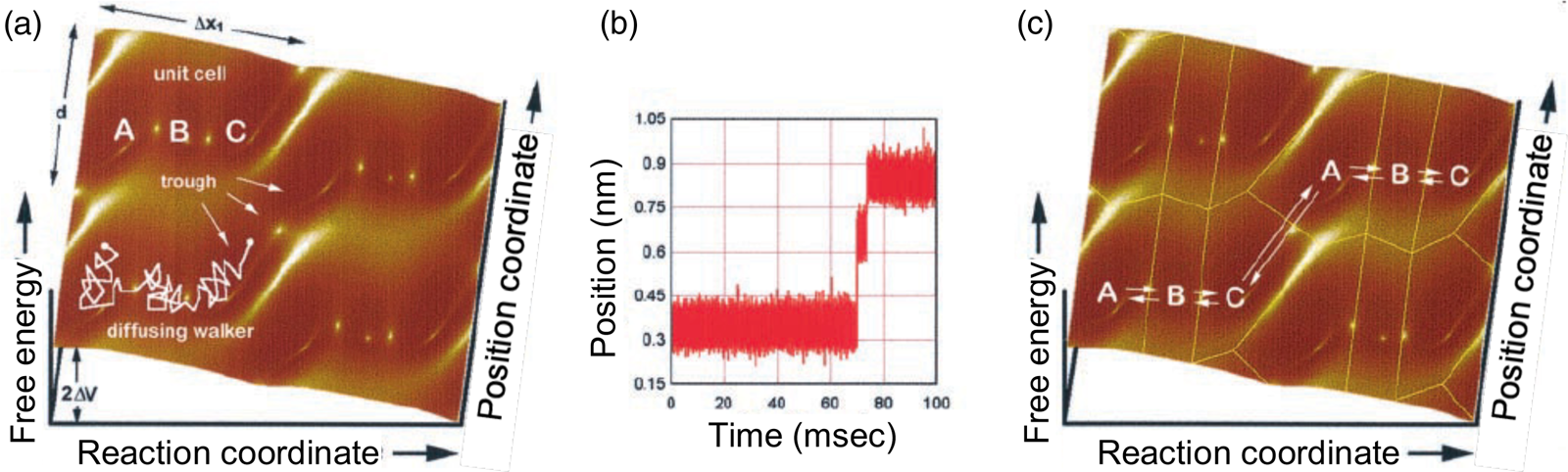
When Jeff Moffitt joined the laboratory as a physics student interested in biophysics, he concentrated his attention in pushing the limits of spatial and temporal resolution of our optical tweezers instrument to extract further information about the phi29 packaging motor. His efforts paid off. Working closely with Yann, Jeff was able to show that the molecular trajectory of the motor was made up of alternating dwell and burst phases. During the dwell (lasting for ~80 ms at saturating [ATP]) the motor does not move, presumably while performing some chemical steps.
During the burst, he showed, the motor translocates the DNA in increments of 10 bp. Significantly, the burst was invariant to whether [ATP] was below or above the motor's K M (40 μM). However, he found that the length of the dwell phase grew inversely proportional to [ATP] (Fig. 32a). This observation immediately implied that the binding of ATP occurs during the dwell. The invariance of the burst size with the [ATP] (Fig. 32a) also indicates a high coordination among the subunits, consistent with what Yann, Aathi, and Jens had observed earlier. Apparently, no subunit fires before all of them have bound ATP, otherwise the burst size would decrease with decreasing [ATP]. But the greatest surprise was still in store. Since the motor is a homo-pentameric ring, the most parsimonious expectation was that each identical subunit packages 2 bp. Indeed, 2 bp is the average number of bp consumed per ATP hydrolyzed in bulk experiments (Guo et al., Reference Guo, Peterson and Anderson1987). Using forces as high as 40 pN to reduce the Brownian noise associated with the fluctuations of the DNA tether Jeff was finally able to observe the stepping of the individual subunits. Much to our surprise, he found that during the burst phase the motor packages the DNA in increments of 10 bp made up not of 5 steps of 2 bp but 4 steps of 2.5 bp! It was a shock. At the beginning I did not believe this result. We were working at what was at the time the limit of our resolution and I thought that this could explain the unexpected result. So, I asked Jeff to repeat the experiments. I still remember that morning when he came to my office and told me: ‘You were right, it is not 2.5 bp it is 2.4 ± 0.1 bp’ (!) Jeff's results indicated that somehow even though all 5 subunits are identical, one of them was not performing the mechanical task of packaging the DNA in each cycle. We did not know what the function of this subunit was, however. We speculated that the discrepancy between the number of bp packaged per ATP hydrolyzed derived from in bulk (in multiplo) and in singulo studies implied that a fifth ATP was being hydrolyzed every cycle – not to perform mechanical movement but for some additional, perhaps regulatory function. Although at the time the discrepancy between experiments bulk and single-molecule experiments remained, our article was accepted for publication in 2009 (Moffitt et al., Reference Moffitt, Chemla, Aathavan, Grimes, Jardine, Anderson and Bustamante2009).
Bacteriophage phi29 packages DNA in bursts of 10 bp, which is composed of four 2.5-bp steps. (a) Representative packaging traces collected under low external load, ~8 pN, and different [ATP]: 250, 100, 50, 25, 10, and 5 μM in purple, brown, green, blue, red, and black, respectively, all boxcar-filtered and decimated to 50 Hz. Data at 1.25 kHz are plotted in light grey. Contour length is plotted in bp of dsDNA. (b) Representative packaging traces collected with external loads of ~40 pN and 250 μM [ATP]. Here data in color are boxcar-filtered and decimated from 1.25 kHz (light gray) to 100 Hz. (c) Average pairwise distribution of packaging traces selected for low noise levels (50% of all packaging data). Inset: force dependence of the observed spatial periodicity. The solid line is the mean for all forces, 2.4 ± 0.1 bp (s.e.m.). Reprinted with permission from Moffitt et al. (Reference Moffitt, Chemla, Aathavan, Grimes, Jardine, Anderson and Bustamante2009).
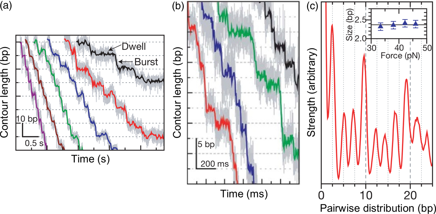
Around the same time another piece of the puzzle was getting in place. Aathi wished to establish what factors determined the grip of the motor toward the DNA substrate. What interactions between the motor and the DNA could account for the large stall forces up to 70 pN observed in our experiments? To this end, he generated DNA molecules harboring varying size (5, 9, 10, 11, 15 and 30 bp) segments of DNA whose phosphates had been neutralized as methyl phosphonates. By selectively neutralizing the Watson or the Crick strand, he showed that during the dwell phase the motor makes contacts with two adjacent DNA phosphates every ten base pairs but only in the strand that is being packaged in the 5′→3′ direction. Significantly, he showed that these DNA contacts had both a load bearing as well as regulatory function in the motor's operation cycle (Aathavan et al., Reference Aathavan, Politzer, Kaplan, Moffitt, Chemla, Grimes, Jardine, Anderson and Bustamante2009).
The next breakthrough occurred when Gheorghe Chistol, a graduate student in Physics, joined the laboratory. At that time, we wished to establish what kind of coordination existed between the subunits of the motor. Recall that Jeff Moffitt had shown that the motor binds ATP during the dwell phase, and Yann Chemla had shown that the motor releases the phosphates from ATP hydrolysis during the burst phase, resulting in the four power strokes from the motor observed by Jeff. Gheorghe now asked: Where in the mechanochemical cycle does the motor hydrolyze ATP? Where in this cycle does the motor release its ADP? And how are these processes coordinated? Joining force with a new postdoctoral fellow Shixin Liu, Gheorghe used ATPγS, a non-hydrolyzable ATP analog, to answer the first question. He found that binding of a single analog is sufficient to induce the motor to pause for several seconds (Fig. 33a). Furthermore, he showed that the induced pauses often appeared as clusters of pauses separated exactly by 10 bp (Fig. 33b). This was a crucial observation. It showed that when one subunit binds the analog and induces pausing, the other four ATP-bound subunits, after pausing for a few seconds, are somehow able to cross a kinetic barrier firing in quick succession one after the other, retaining their coordination and producing a 10 bp burst, only to enter another long pause. This process repeats until the subunit bound to the analog exchanges it for ATP, wherein the motor can resume its normal operation. Importantly, Gheorghe also found that the burst sizes that preceded an ATPγS-induced pause could be 2.5, 5.0, 7.5 and 10 bp (Fig. 34) as would be expected if the hydrolysis of ATP occurred during the burst. To answer the second question, Gheorghe used Na+-orthovanadate, a compound that prevents the release of an ADP that is bound to the motor. As it turns out, preventing the release of ADP also induced a pause in the motor, indicating that the release of ADP was also a coordinated process among the subunits. Interestingly, in this case the burst size that preceded the orthovanadate-induced pause was always 10 bp away from the pause, indicating that the release of ADP happens during the dwell phase. Since we knew that binding of ATP also occurs in the dwell, we wondered whether these two events are somehow coordinated. To answer this question, we noticed that even though the operation of the five subunits is highly coordinated, the Hill analysis of ATP hydrolysis by the motor yielded a Hill coefficient n Hill = 1. This result was totally unexpected. How could a pentameric ATPase whose subunits bind and hydrolyze ATP in a coordinated manner – implying a great degree of communication among them around the ring – behaves as a non-cooperative system? We realized that there was only one possible scheme that could account for this ‘apparent’ lack of cooperativity among the subunits, and that was if the binding of ATP and the release of ADP are interlaced processes. In this scenario, the release of ADP by a subunit allows that subunit to bind one ATP, which in turn induces the release of the ADP in the next subunit, which can then bind an ATP, and so on. Therefore, even though the motor is pentameric and can bind up to 5 ATPs in a coordinated fashion, at any given time it has only one site available to bind ATP, thus resulting in an n Hill = 1. Moreover, in this study Gheorghe showed that the special subunit, i.e., the one that does not do any mechanical work, also binds and hydrolyzes ATP. This additional observation resolved the prior discrepancy between in multiplo and in singulo studies: 5 ATPs are consumed in every operation cycle, but only 4 of them are involved in the mechanical movement of DNA during packaging (Chistol et al., Reference Chistol, Liu, Hetherington, Moffitt, Grimes, Jardine and Bustamante2012).
Non-hydrolyzable ATP analog induces pausing events. (a) Packaging traces at saturating [ATP] (250 μM) and various amounts of ATPγS. (b) ATPγS-induced pausing events consist of one or more pauses separated by 10-bp bursts. Pausing events are characterized by their duration (orange bar) and span (the length of DNA translocated during an event, green bar). Pausing events consisting of two or more pauses are referred to as pause clusters. Reprinted with permission from Chistol et al. (Reference Chistol, Liu, Hetherington, Moffitt, Grimes, Jardine and Bustamante2012).
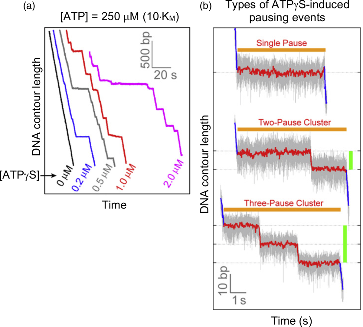
Determining the timing of ATP hydrolysis in the dwell-burst cycle. Detailed view of four sample packaging traces containing an ATPγS-induced pausing event, from 40 bp upstream of the pausing event to 0.5 s after the start of the pausing event. Regular packaging is shown in blue, and the start of the pausing event is shown in red. The large peak (red arrowhead) in the residence time histogram corresponds to the start of the pausing event. Two regular dwells (blue arrowheads) were used as anchors for aligning different residence time histograms. Reprinted with permission from Chistol et al. (Reference Chistol, Liu, Hetherington, Moffitt, Grimes, Jardine and Bustamante2012).
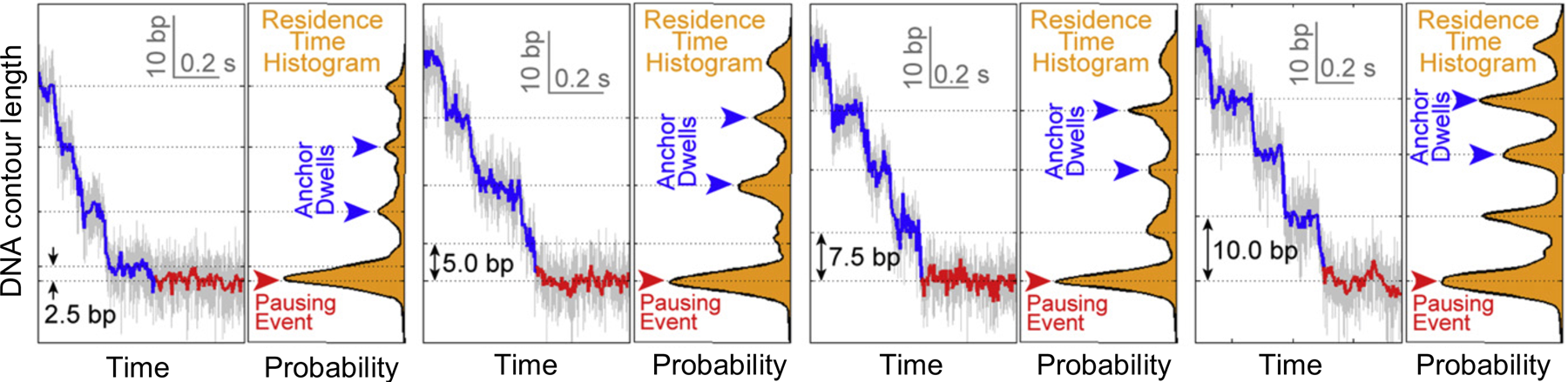
What is the role of the special subunit? Is it the same cycle after cycle, or does it vary from cycle to cycle? We knew that when one of the subunits is bound to ATPγS, the other subunits still retain the ability to hydrolyze their ATP in a coordinated fashion, just that they stall for a long time before packaging 10 bp of DNA only to enter another long pause. It is as if, when one of the subunits is bound to the analog nucleotide, the other subunits are waiting for a signal in order to hydrolyze their ATPs and package the DNA, but that signal never arrives. Eventually, during the long wait, one of the subunits experiences a fluctuation that allows it to spontaneously cross the catalytic barrier, and this event triggers the coordinated firing of the other subunits, thus giving rise to a 10-bp burst. Gheorghe's data could be explained if we hypothesize that the subunit that binds the ATPγS automatically adopts the identity of the special subunit and that the function of this subunit is to hydrolyze ATP in order to signal to the other subunits that they must start firing.
Sara Tafoya, a biophysics graduate student, then joined the laboratory and began to work with Gheorghe. She became interested in developing mutants that could affect the inter-subunit coordination of the motor. Sara targeted arginine R146 that we thought could play a role in that coordination and she showed that when the motor contained one mutant (R146A) subunit, it exhibited the same characteristic as a motor that had one ATPγS bound (Tafoya et al., Reference Tafoya, Liu, Castillo, Atz, Morais, Grimes, Jardine and Bustamante2018), except that here the phenotype was permanent and constitutive of this mutant motor (Fig. 35).
Packaging behavior of hybrid motors containing one R146A mutant subunit out of 5. Left: high-resolution packaging trajectories of WT (blue) and slow R146A/WT hybrid motors from a mixture containing 20% mutant subunits (red). Right: sample packaging trajectory of WT motors in the presence of the non-hydrolyzable nucleotide ATPγS in a 1:500 ([ATP]:[ATPγS]) ratio. ATPγS-induced pauses are highlighted in red; regular packaging behavior is in blue. Reprinted with permission from Tafoya et al. (Reference Tafoya, Liu, Castillo, Atz, Morais, Grimes, Jardine and Bustamante2018).
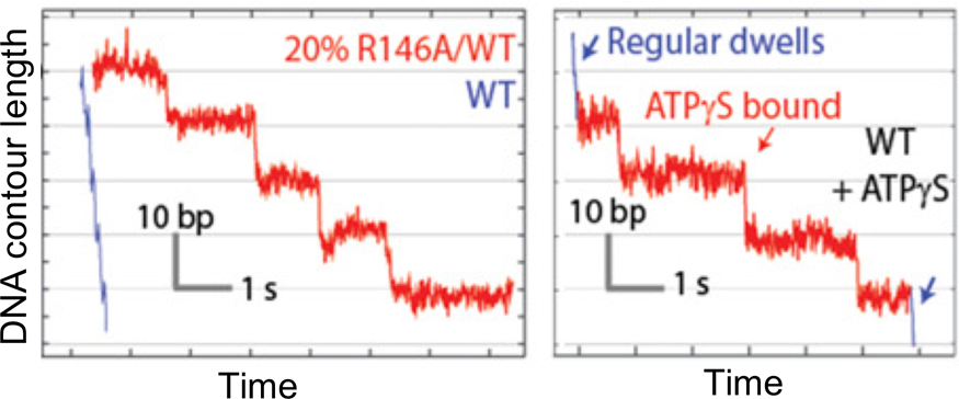
This observation strongly supports our hypothesis that the subunit unable to hydrolyze ATP adopts the identity of the special ‘regulatory’ subunit. This subunit, which under normal conditions is the master regulator of the cycle, in the case of the mutant motor, is unable to send the signal that the other subunits need to start firing and packaging, giving rise to packaging trajectories made up of long pauses separated by 10 bp.
Finally, we asked: under normal operating conditions (i.e., no ATPγS and no arginine mutation), what event determines the identity of the special subunit within the motor? In other words, what event breaks the symmetry of the motor? Moreover, is this identity retained by the same subunit from cycle to cycle? Shixin, in collaboration with physics graduate student Craig Hetherington, Gheorghe, Sara, and Aathi, decided to answer these questions. First, in extremely difficult experiments, Craig was able to show that the phi29 motor not only can generate force, but it can also introduce torque into the DNA during motor packaging. To make sure that the rotation observed was not due to the coiling of the DNA inside the capsid, we ‘trepaneted’ the viral heads by freezing and thawing them before the packaging assay. In this way, DNA entered at the base of the capsid and left by one of the wholes made by the ice crystal during freezing. He used a modified rotor bead assay as shown in Fig. 36a to show that the motor in trepanated phage heads rotates the DNA by 1.5 ± 0.2o bp–1. Furthermore, Craig had found that the amount of rotation per base pair increases with the fraction of the genome packaged (Fig. 36b). Meanwhile, Shixin had determined that as the DNA fills the capsid, and more than 80% of the genome has been packaged, the size of the burst steadily begins to decrease from 10 bp at zero filling to 9 bp at 100% filling (Fig. 36c) presumably due to the pressure buildup. We suspected that these parallel changes were not coincidental but related to each other. With all these data in hand, we were able to formulate the following model for the operation of the phi29 DNA packaging motor. We proposed that the special subunit is the one that contacts the pair of phosphates at the end of the 10-bp burst (at low capsid filling) every cycle. This is the event that breaks the symmetry of the motor. That subunit will adopt the regulatory role in the cycle and will not perform a mechanical task. Note, however, that while the burst size is 10 bp, the periodicity of the dsDNA is 10.4 bp. As a result, at the end of each packaging burst, the phosphodiester backbone of dsDNA has rotated not by a full turn of 360° (as it would be required for the special subunit of the previous cycle to contact again the phosphates in DNA and retain its identity during the next cycle) but only by 346°. Therefore, in order for the special subunit to retain its regulatory identity and successively contact the phosphates cycle after cycle, the packaging motor must actively rotate the dsDNA substrate by 14 degrees in every 10-bp burst, or 1.4° bp–1, which is very close to the rotation density Craig detected experimentally. Even more surprisingly, we noticed that the increase in rotation per base pair observed with increased capsid filling precisely matched the additional rotation needed to compensate for the reduction in burst size by the motor (i.e., drop from 10 to 9 bp), thereby permitting the same special subunit remain in contact with the dsDNA substrate and continue to regulate the mechanochemical cycle of the packaging motor (Fig. 37b and c) (Liu et al., Reference Liu, Chistol, Hetherington, Tafoya, Aathavan, Schnitzbauer, Grimes, Jardine and Bustamante2014b).
phi29 motor rotates DNA during packaging. (a) Experimental geometry of the rotation assay. The packaging complex is tethered between two beads. Biotin-streptavidin linkages torsionally couple the rotor bead to the optically trapped bead via dsDNA. A nick and an ssDNA region ensure that the rotor bead is torsionally decoupled from the micropipette-bound bead. (b) Local DNA rotation density (ρ) versus capsid filling. The data point obtained with trepanated proheads – corresponding to very low capsid filling conditions – is shown as a magenta square. Error bars represent s.e.m. (c) Mean burst size versus capsid filling, which was found to modulate the step size of the motor without affecting subunit coordination. Error bars represent 95% CI. The ρ values can also be inferred from the observed burst sizes, as shown in panel B (gray). Reprinted with permission from Liu et al. (Reference Liu, Chistol, Hetherington, Tafoya, Aathavan, Schnitzbauer, Grimes, Jardine and Bustamante2014b).

Corrected internal force as a function of capsid filling. Comparison with Fig. 30c shows that the magnitude of this force reaches ~20–25 pN at the end of packaging. Reprinted with permission from Liu et al. (Reference Liu, Chistol, Hetherington, Tafoya, Aathavan, Schnitzbauer, Grimes, Jardine and Bustamante2014b).
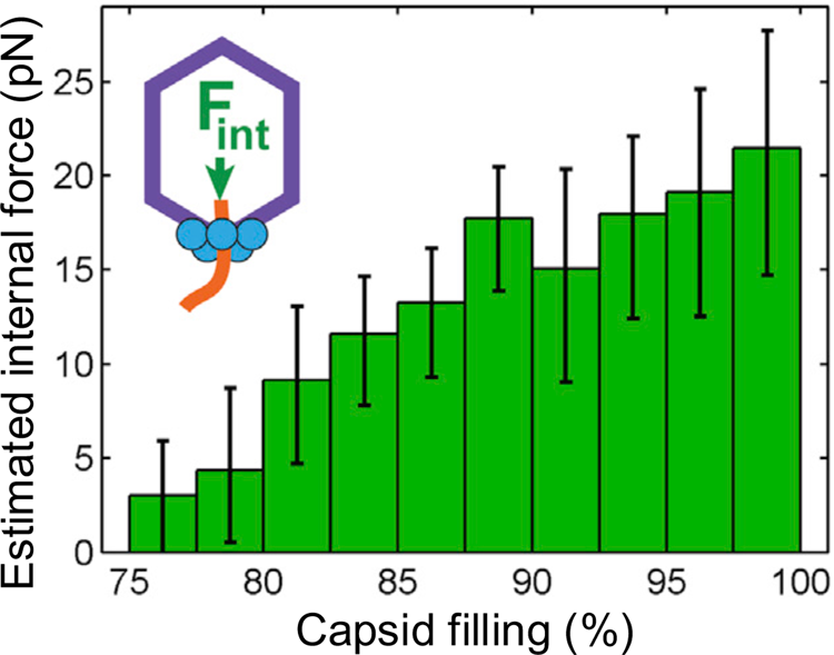
Incidentally, Shixin's work at high capsid filling revealed that the effect of the internal force resulting from the accumulated pressure was not equivalent to that of the external force applied with the tweezers. Whereas the external force only slows down the burst phase, he found that the internal force lengthens both the burst and the dwell phases. In Fig. 30b, this equivalence is assumed, namely that the internal force, like the externally applied one, only affects the burst phase. Accordingly, in our earlier work the effect of the internal force had been underestimated as it takes half of the internal force to slow down the packaging rate to the extent observed experimentally. Thus, Fig. 30c, where the rate is used to estimate the internal force under the equivalence assumption, results in an overestimation in the calculated internal force developed toward the end of packaging by ~30 pN. Figure 37 depicts the correct increase of the internal force with the percent capsid filling.
Figure 38 summarizes the full scheme of the mechanochemical cycle that we have established over decades of work for the phi29 DNA packaging motor.
Mechanochemical model of the dwell-burst cycle by the phi29 packaging motor at low capsid filling (Liu et al., Reference Liu, Chistol, Hetherington, Tafoya, Aathavan, Schnitzbauer, Grimes, Jardine and Bustamante2014b). The dwell phase (red line) and the burst phase (four 2.5-bp steps in green) are depicted together with the chemical processes that take place in them. In this model, rotation is assumed to occur at the end of the burst and the beginning of the next dwell phase, which coincides with the engagement of the DNA phosphates by the special subunit, triggering the beginning of a new cycle.
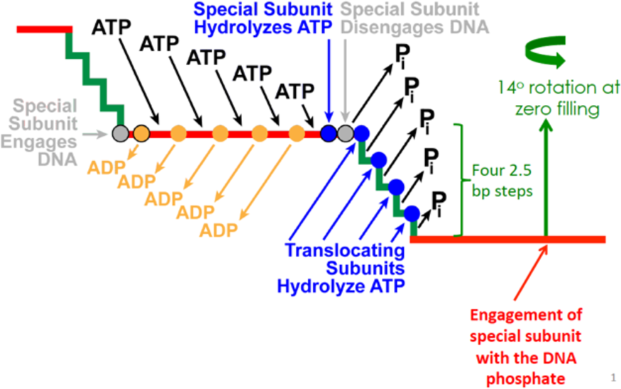
Bacterial protease
ATP-dependent proteases of the AAA+ superfamily power the degradation of misfolded, denatured, or otherwise damaged polypeptides and the removal of short-lived regulatory proteins (King et al., Reference King, Deshaies, Peters and Kirschner1996). These peptidases pair with energy-dependent hexameric AAA+ unfoldases, which recognize appropriately tagged protein substrates and use the energy of ATP hydrolysis to unfold and translocate the polypeptide into the peptidase chamber for degradation (Wang et al., Reference Wang, Hartling and Flanagan1997a; Baker and Sauer, Reference Baker and Sauer2006). Hexameric AAA+-ATPase rings include the 26S proteasomes in eukaryotic cells, the prokaryotic HsIU AAA+-ATPase which operates with the HsIV protease composed of two homohexameric rings, the E. coli ClpX associated with ClpP, a AAA+ protease that organizes as heptameric double rings, as well as corresponding homologs in archaea (Grimaud et al., Reference Grimaud, Kessel, Beuron, Steven and Maurizi1998; Baker and Sauer, Reference Baker and Sauer2012).
Despite extensive structural, biochemical, and initial single-molecule fluorescence studies of ClpX (Shin et al., Reference Shin, Davis, Brau, Martin, Kenniston, Baker, Sauer and Lang2009), direct evidence for force generation and a detailed characterization of the mechanochemistry of these machines had been lacking. Rodrigo Maillard, a postdoctoral fellow who had joined the laboratory at the time, became interested in studying this protein. As luck would have it, my colleague Andreas Martin, who had done a very elegant biochemical characterization of this enzyme in Robert Sauer's laboratory at MIT, had just joined the Molecular and Cell Biology Department here at Berkeley. We agreed to collaborate on this project.
ClpX recognizes proteins with a C-terminal ssrA tag and is known to use cycles of ATP hydrolysis to unfold and translocate the substrates into its associated peptidase, ClpP (Gottesman et al., Reference Gottesman, Roche, Zhou and Sauer1998). In our studies we designed a single-molecule optical tweezers-based assay to investigate force generation in ClpX – both alone and in complex with its peptidase ClpP (Fig. 39a). The substrate was a fusion of an unfolding titin molecule and a folded GFP. Rodrigo showed that ClpX functions as a molecular motor, generating force to unfold and translocate its substrates through its central pore (Fig. 39b–e). He found that polypeptide threading is interrupted by pauses off the main translocation pathway, and that ClpX's translocation velocity is force dependent, reaching a maximum of 80 aa s–1 near zero force and vanishing above 20 pN (aa: amino acid). The motor displayed bursts of 1, 2, or 3 nm, suggesting a fundamental step-size of 1 nm per subunit, consistent with high-resolution crystallographic data (Glynn et al., Reference Glynn, Martin, Nager, Baker and Sauer2009). Binding of ClpP decreases the probability of slippage and enhances the unfolding efficiency of ClpX. Under the action of ClpXP, GFP unfolds cooperatively via a transient intermediate (red square in Fig. 39e). Our results appeared in Cell (Maillard et al., Reference Maillard, Chistol, Sen, Righini, Tan, Kaiser, Hodges, Martin and Bustamante2011) almost simultaneously with a similar study by the groups of Robert Sauer and Tania Baker (Aubin-Tam et al., Reference Aubin-Tam, Olivares, Sauer, Baker and Lang2011). Gratifyingly, the results were nearly identical despite being obtained independently.
Unfolding and translocation of GFP-titin fusion proteins by ClpX and ClpXP. (a) Geometry of assay: ClpX(P) was immobilized on a streptavidin polystyrene bead (SA). The GFP-titin fusion substrate is covalently linked to a 3-kbp dsDNA handle with a Dig tag that binds to an antibody-coated polystyrene bead (AD). All substrates included one or two GFP molecules (green) fused to a chemically-unfolded Ti-ssrA moiety (red and black). The blue flexible linker corresponds to the ybbR tag. (b–d) Molecular traces showing GFP unfolding as a sudden increase of tether length (red arrowheads), followed by gradual shortening (negative slope regions) upon motor translocation, where sometimes motor slippages occur (black arrowhead). aa, amino acid. (b) Single GFP-titin substrate. (c) Double GFP substrate with a short linker (10 aa) between the GFP molecules. (d) Double GFP substrate with a long flexible linker of 200 aa between the GFP molecules. (e) Characteristic features of GFP unfolding by ClpXP: the motor ‘pauses’ before GFP unfolds cooperatively via a transient intermediate state (red square) and is ‘ripped’ into an extended polypeptide chain, along which the motor then steadily ‘translocates’ and ‘pauses’ again when nearing the end of the chain. Reprinted with permission from Maillard et al. (Reference Maillard, Chistol, Sen, Righini, Tan, Kaiser, Hodges, Martin and Bustamante2011).
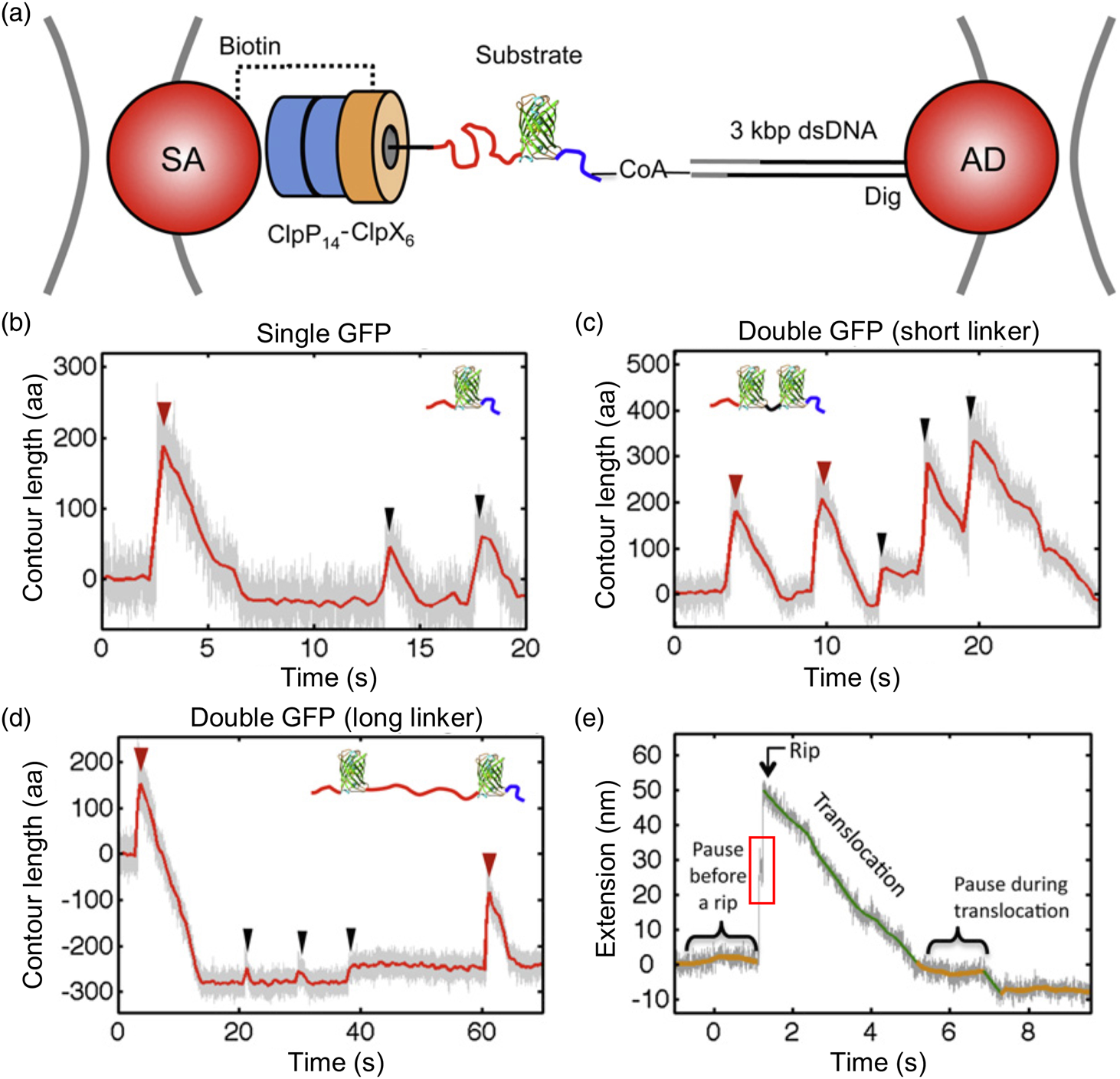
Following these initial studies, Maya Sen, a graduate student in the laboratory decided to investigate the mechanism of force generation and inter-subunit coordination in ClpXP (Sen et al., Reference Sen, Maillard, Nyquist, Rodriguez-Aliaga, Presse, Martin and Bustamante2013). Using the same single-molecule assay, she showed that the molecular trajectories of the motor over an unfolded polypeptide are made of alternating dwells and bursts (Fig. 40). Moreover, Maya found that the dependence of the rate of translocation on [ATP], [ADP], and [Pi] indicates that the power stroke of this motor coincides with the release of phosphate. Although this protease is a homohexameric ring, two of the subunits do not seem to perform a mechanical task, as the majority of bursts are of 2, 3, and 4 nm, but not larger. The distribution of burst sizes varies with [ATP] and probably reflects the near-instantaneous coordinated firing of 2, 3, or 4 subunits around the ring. In fact, previous biochemical and structural studies show that at most four subunits in the hexamer can bind ATP at any given time (Glynn et al., Reference Glynn, Martin, Nager, Baker and Sauer2009; Hersch et al., Reference Hersch, Burton, Bolon, Baker and Sauer2005; Stinson et al., Reference Stinson, Nager, Glynn, Schmitz, Baker and Sauer2013). Consistently, she found that the motor can still function with up to two non-hydrolyzable ATPγS analog nucleotides bound to it. Taken together, these data suggest that the operation of ClpXP subunits is less coordinated than those of bacterial phage phi29 packaging motor.
Molecular trajectories of ClpXP during translocation over an unfolded polypeptide and depicting alternating dwells and bursts at saturating (blue) and limiting (red) [ATP]. Figure adapted and reprinted with permission from Sen et al. (Reference Sen, Maillard, Nyquist, Rodriguez-Aliaga, Presse, Martin and Bustamante2013).
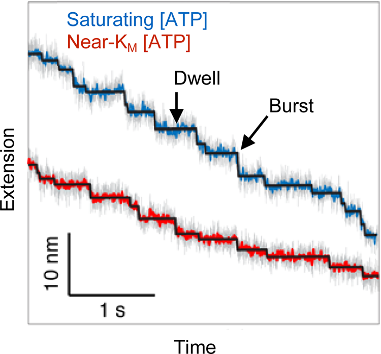
As Maya Sen was finishing her doctorate, Piere Rodríguez joined the laboratory and declared his interest in working on the ClpXP system. Using the same single-molecule assay as Rodrigo and Maya, he set himself to characterize ClpXP's mechanochemical cycle. Piere found that ADP release and ATP binding occur non-sequentially during the dwell, while ATP hydrolysis and phosphate release occur during the burst; moreover, he established that ADP release is the rate-limiting chemical transition in the dwell.
Pore loops of ClpXP and other AAA+ proteases contact and propel their substrate. To establish why their loop sequence (GYVG) is so highly conserved from bacteria to humans, Piere mutated them and found that loop mutants with side chains smaller than the wild-type (WT), compromise their traction on the polypeptide chain, thus reducing the motor's mechanochemical coupling efficiency (nm per ATP) (Fig. 41); similarly, mutants harboring residues larger than WT compromise the velocity of the motor by making the movement of the loops slower, presumably due to steric hindrance at the lumen (Fig. 41). Since the motor's power output is the product of the force that the loops can exert on the substrate (grip) times their velocity, he found that the sequence GYVG in the WT ClpXP motor has evolved to provide an optimum of power output and coupling efficiency by involving amino acid side chains that minimize steric hindrance (maximazing pulling velocity) without compromising their grip (force generation) (Fig. 42) (Rodriguez-Aliaga et al., Reference Rodriguez-Aliaga, Ramirez, Kim, Bustamante and Martin2016).
Coupling coefficient between substrate translocation and ATP consumption for wildtype (WT) ClpXP and GYVG mutants of increasing bulkiness (mean ± s.e.m.) at 5 mM ATP. The coupling coefficient is maximum for the WT motor. Reprinted with permission from Rodriguez-Aliaga et al. (Reference Rodriguez-Aliaga, Ramirez, Kim, Bustamante and Martin2016).

Schematic depiction of the optimization of the mechanochemical power efficiency of the motor and its power output by the size of the side chains of the translocating loops. Because power = force × velocity, decreasing the bulkiness of the side chain loops increases the translocation velocity but at the expense of decreasing the grip on the substrate and the force production of the motor. Similarly, increasing the loops' bulkiness increases their grip on the substrate at the expense of reducing their velocity due to steric hindrance. The wild-type (WT) loops reside at the maximum predicted by this product, maximizing the efficiency of mechanochemical coupling and the power output of the motor. Figure adapted and reprinted with permission from Rodriguez-Aliaga et al. (Reference Rodriguez-Aliaga, Ramirez, Kim, Bustamante and Martin2016).
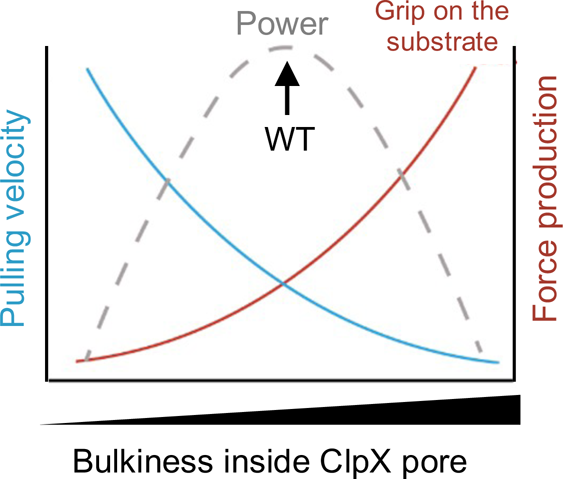
Translation studies
Ribosomes are the cellular machines that effect the translation from the language of nucleotide sequences into that amino acid sequences (Moore and Steitz, Reference Moore and Steitz2003). The prokaryotic ribosomes are made up of two subunits: the large or 50S subunit made up of 2 RNA molecules (5S and 23S RNA) and 31 proteins, and the small or 30S subunit made up of one 16S RNA molecule and 21 proteins. The translation process is conveniently divided into three phases: initiation, elongation, and termination. At the beginning of the process, initiation factors IF1, IF2.GTP, and IF3 are involved in delivering the small subunit into the methionine-encoding mRNA translation start codon, AUG, whose placing at the P site of the small subunit is directed by an upstream Shine–Dalgarno (SD) sequence complementary to a segment of the 16S ribosomal RNA (Kaminishi et al., Reference Kaminishi, Wilson, Takemoto, Harms, Kawazoe, Schluenzen, Hanawa-Suetsugu, Shirouzu, Fucini and Yokoyama2007; Korostelev et al., Reference Korostelev, Trakhanov, Asahara, Laurberg, Lancaster and Noller2007; Bustamante et al., Reference Bustamante, Cheng and Mejia2011). Once bound to the start site of translation, the small subunit recruits the larger subunit and the A, P, and E tRNA sites of the ribosome are thus completed. During the elongation phase, elongation factor Tu (EF-Tu) bound to GTP brings the tRNA charged with the correct amino acid and places it in the A site. Here the tRNA uses its complementarity to the codon on the mRNA and its interactions with the small and large subunits. Then, EF-Tu hydrolyzes its GTP and releases from the ribosome, leaving the tRNA bound in the ‘classical’ position at the A site. This tRNA is adjacent to the peptide-containing tRNA bound in the classical position at the P site. The proximity of the polypeptide in the P site and the new amino acid in the A site permits the formation of a new peptide bond and the polypeptide in the P site is transferred to the A site tRNA, a reaction catalyzed by the peptidyl transferase activity of the 23S rRNA in the active site of the 50S subunit. At this point, the rotation between the large and small subunit allows the tRNAs to access intermediate binding conformations called ‘hybrid’ states, in which the anticodon ends of the tRNAs remain in their classical A and P sites in the 30S subunit but their acceptor stems make now contacts in the P and E sites of the 50S subunit, respectively (Moazed and Noller, Reference Moazed and Noller1989; Frank and Agrawal, Reference Frank and Agrawal2000; Cornish et al., Reference Cornish, Ermolenko, Noller and Ha2008; Zhang et al., Reference Zhang, Dunkle and Cate2009; Sharma et al., Reference Sharma, Adio, Senyushkina, Belardinelli, Peske and Rodnina2016). This hybrid state is the preamble for a critical step in the translation cycle which requires the binding of the GTP-bound elongation factor G (EF-G), a GTPase that catalyzes the rotation of the head domain of the small subunit and the translocation of the mRNA and its bound tRNAs from the A and P sites, to the P and E sites respectively. Finally, termination takes place when the ribosome encounters a stop codon (UAA, UGA, or UAG). Either the release factor 1 (RF1) or the release factor 2 (RF2) recognize the UAA and UAG or UAA and UGA, respectively, and cleave the peptide from the tRNA at the P site.
Optical tweezers have been used to evaluate the mechanical strength of the mRNA binding to the ribosome under different conditions (Uemura et al., Reference Uemura, Dorywalska, Lee, Kim, Puglisi and Chu2007). The force required to pull the mRNA from the ribosome increased by ~5 pN when deacylated tRNAfMet was bound to the P site. A Phe-tRNAPhe bound at the A site, on the other hand, stabilized the P-site-bound ribosome by ~10 pN. A SD sequence further strengthened the interaction by ~10 pN, but a peptidyl-tRNA analog N-acetyl-Phe-tRNAPhe bound to the A site weakened the rupture force in an SD-independent manner relative to the complex carrying a Phe-tRNAPhe, indicating that following peptide bond formation, the ribosome loses grip of the mRNA to complete translocation.
Around this time, our group, and the group of Nacho Tinoco decided to develop an RNA hairpin assay to follow translation by a single ribosome. We wished to characterize the mechanism of translocation of the ribosome and its helicase activity. Two postdoctoral associates, Jin Der Wen and Ana Carolina Zeri got to work on developing the assay, in collaboration with Harry Noller and Laura Lancaster at the University of California in Santa Cruz. In these experiments, either a 60-bp or a 274-bp hairpin is tethered via RNA/DNA hybrid segments to a bead held in optical trap and to a bead held by suction atop a micropipette (Fig. 43a). An AUG site is placed at the base of the hairpin to which a single ribosome can bind. To reduce the complexity of the biochemical reactions involved during translation, the hairpin only contained codons corresponding to interspersed runs of glutamic acid and valine. When the tRNAs are added to the optical tweezers chamber, the ribosome begins to move and invade the hairpin. The experiment is done using force feedback. In this way, for each codon translated, the end-to-end distance of the RNA hairpin increases by six nucleotides, which under the tension applied (~18 pN) requires the traps to be moved apart by ~2.7 nm to keep the tension constant. The molecular trajectories obtained in this way (Fig. 43b) depict single codon steps interspersed by dwells of variable duration during which the ribosome does not move (Wen et al., Reference Wen, Lancaster, Hodges, Zeri, Yoshimura, Noller, Bustamante and Tinoco2008). The distribution of dwell lengths, with a median of 2.8 s, revealed that at least two rate-determining processes control each dwell. The rate of translation reached values of 0.45 codon s−1. The fact that translocation steps are exactly one codon indicates that translocation and RNA unwinding (helicase activity) are strictly coupled ribosomal functions. This study also revealed that the ribosome displays long pauses lasting from tens of seconds up to 1–2 min. We found that many of these long pauses were correlated with internal SD sequences in the mRNA with which, presumably the RNA in the 30S subunit hybridizes to induce the pause.
(a) Experimental design of RNA hairpin unwinding assay for monitoring a single ribosome codon-by-codon translation in real-time. The ribosome was stalled at the 5′ side of the mRNA hairpin construct, which was then held between two polystyrene beads. Drawings are schematic and not to scale. (b) Extension and force trajectories during translation. The data were collected at 200 Hz (blue traces) and smoothed to 10 Hz (red). Discrete steps are indicated by arrowheads. The 18 nm rip at 163 s corresponds to spontaneous opening of the remaining approximately 18-bp hairpin ahead of the translating ribosome. Reprinted with permission from Wen et al. (Reference Wen, Lancaster, Hodges, Zeri, Yoshimura, Noller, Bustamante and Tinoco2008).
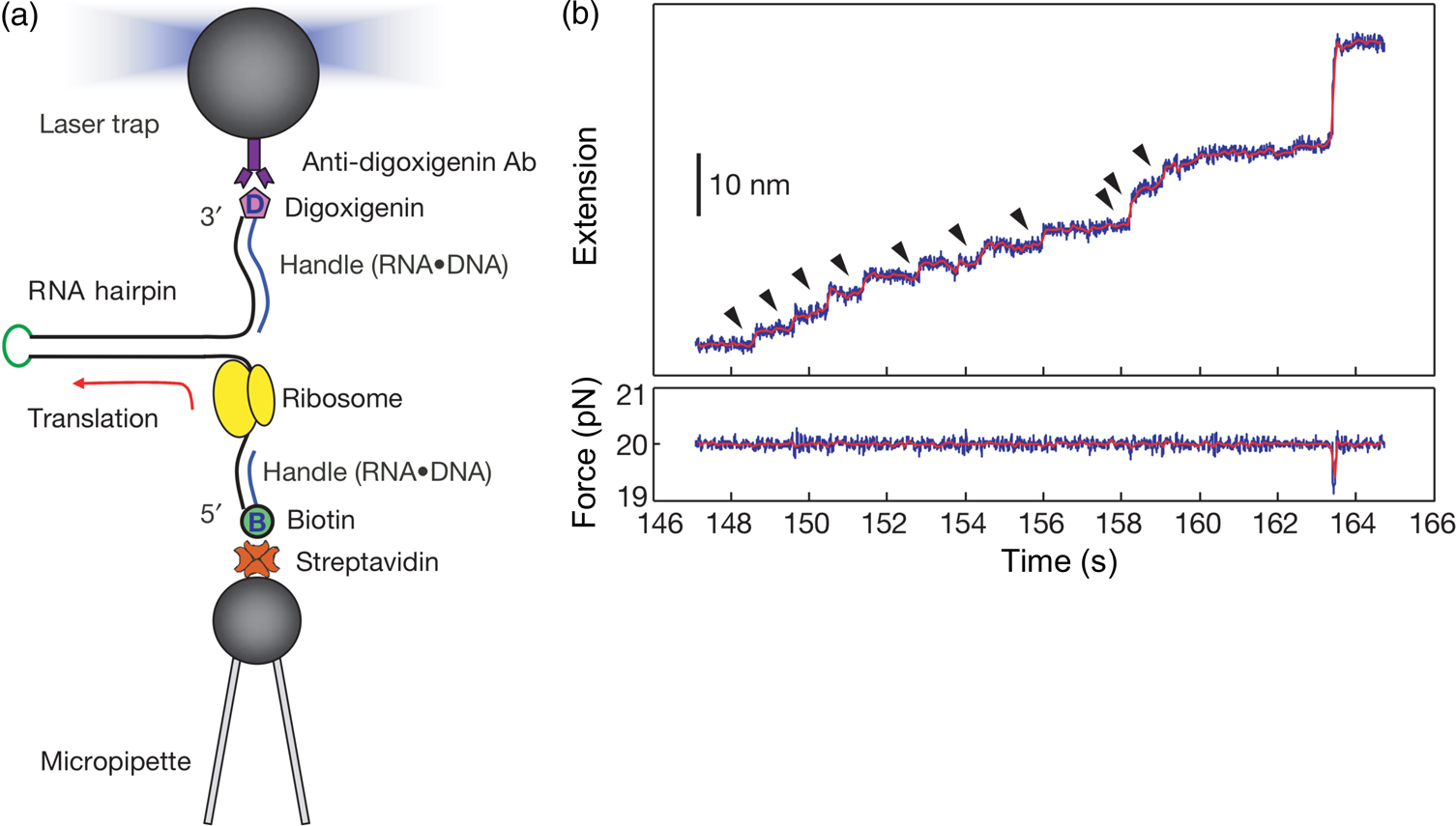
The RNA assay used in our initial translation studies did not permit us to investigate the mechanical or motor properties of the ribosome. Ting Ting Liu and Ariel Kaplan, two postdoctoral associates, agreed to collaborate in an experiment to measure the stall force of the ribosome. To this end, they developed a ‘tug-of-war’ assay in which we could apply varying mechanical loads to the ribosome. The geometry of the experiment is depicted in Fig. 44a. In this experiment the optical trap position is kept constant relative to the bead atop the micropipette so that as the ribosome translates the mRNA, it pulls the bead off the center of the trap and experiences an increasing force. We found that the ribosome velocity is extremely sensitive to the external load and decays exponentially with the force (Fig. 44b) (Liu et al., Reference Liu, Kaplan, Alexander, Yan, Wen, Lancaster, Wickersham, Fredrick, Noller, Tinoco and Bustamante2014c). Fit of the data to the generalized Arrhenius equation (Eq. (16)) yields a zero-force velocity v 0 = 2.9 codon s−1 (1.8, 4.0) and a distance to the transition state of 1.4 nm (0.9, 1.8), nearly the size of one full codon (the numbers in parenthesis indicate 95% confidence bounds). Ting Ting and Ariel found that the stall force of the ribosome is ~13 pN (Fig. 44b), barely capable of unwinding the most stable secondary structures in mRNAs, thus establishing the physical basis for the latter's regulatory role in translation.
(a) Experimental design for a ‘tug-of-war’ geometry of single-molecule translation assay. A biotinylated ribosome is loaded onto a single-stranded mRNA and attached to a streptavidin-coated polystyrene bead fixed to a micropipette. The mRNA 3′-end is anchored to a second bead through a 1460-bp DNA/RNA hybrid handle. Calibrated forces can be applied to the ribosome by manipulating the second bead with an optical trap, while the translation progress of the ribosome is determined by the change in extension of the tether. (b) Pause-free translational velocity as a function of opposing force. Data points are the mean velocities for all measured traces at each force (N = 54). Error bars represent s.e.m. The solid line is an exponential fit as: $\nu ( F) = \nu _0\exp ( {-( F\cdot \tilde{x}) /( \kappa_BT) } )$ . Reprinted with permission from Liu et al. (Reference Liu, Kaplan, Alexander, Yan, Wen, Lancaster, Wickersham, Fredrick, Noller, Tinoco and Bustamante2014c).
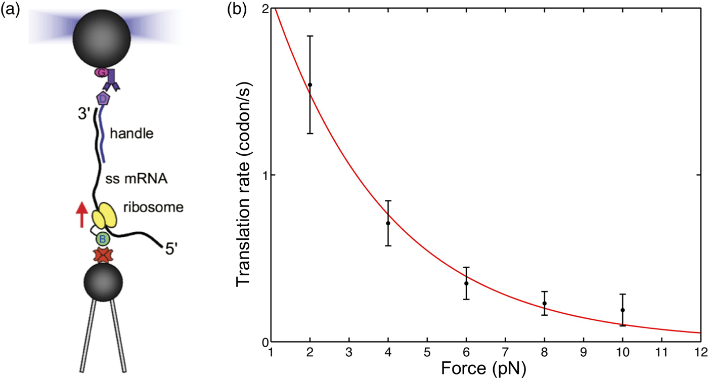
When Shannon Yan, co-author of this article, joined Nacho Tinoco's laboratory as a chemistry graduate student, she became interested in understanding the molecular determinants of program ribosomal frameshift, a process by which the cell can produce alternative proteins from a single transcript. During programmed frameshift, the ribosome can access either of the two out-of-frames (−1 and +1), greatly expanding the gene coding capacity of a transcript. Program frameshift plays an important role in bacteria and in viruses such as HIV-1 where successive frameshifts are needed to synthesize the retroviral polyprotein (Jacks et al., Reference Jacks, Power, Masiarz, Luciw, Barr and Varmus1988). We decided to investigate the programed frameshift in E. coli dnaX gene involved in the synthesis of the γ and τ subunits of DNA polymerase III (Tsuchihashi and Brown, Reference Tsuchihashi and Brown1992). Program frameshift involves three sequence elements: a slippery sequence AAAAAAG flanked by an internal SD sequence located 10 nt upstream and an 11-bp hairpin 6 nt downstream. Combining mass spectrometry of the synthesized protein and single ribosome molecular trajectories using optical tweezers, she was able to show that ribosomes enter the −1 frame from multiple alternative codons along the slippery sequence and slip by not just −1 but also −4 or +2 nucleotides. Correspondingly, the single ribosome trajectories display codon-size excursions over the slippery sequence corresponding to multiple ribosome translocation attempts during frameshift (Fig. 45). These large excursions probably result from the combined mechanical contributions of the SD sequence that pulls back on the advancing ribosome, the downstream hairpin that represents a barrier for its forward translocation, and the slippery sequence over which it diffuses before re-engaging on a new frame (Yan et al., Reference Yan, Wen, Bustamante and Tinoco2015).
A single-ribosome translation trajectory along the frameshift-promoting wild-type slippery sequence (S.S., orange-shaded area). Data taken with the same RNA hairpin unwinding assay as in Fig. 43a, recorded at 1 kHz, and displayed here at 20 Hz. Upon each translocation step by the ribosome (vertical advances along y-axis, indicated by black arrowheads), the hairpin releases 6 nt per codon, resulting in 2.65 nm increment (spacing between gridlines of the same color) in mRNA end-to-end extension under a constant tension of 18 pN. According to the mRNA sequence, amino acids (letter codes) incorporated by the P-site tRNA after each translocation step are labeled next to the gridlines (green for 0 frame, purple for −1 frame). As the ribosome continually translocates, characteristic fluctuations in mRNA extension (bottom zoom-in) were detected downstream from the internal Shine–Dalgarno sequence and around the slippery sequence region. Reprinted with permission from Yan et al. (Reference Yan, Wen, Bustamante and Tinoco2015).
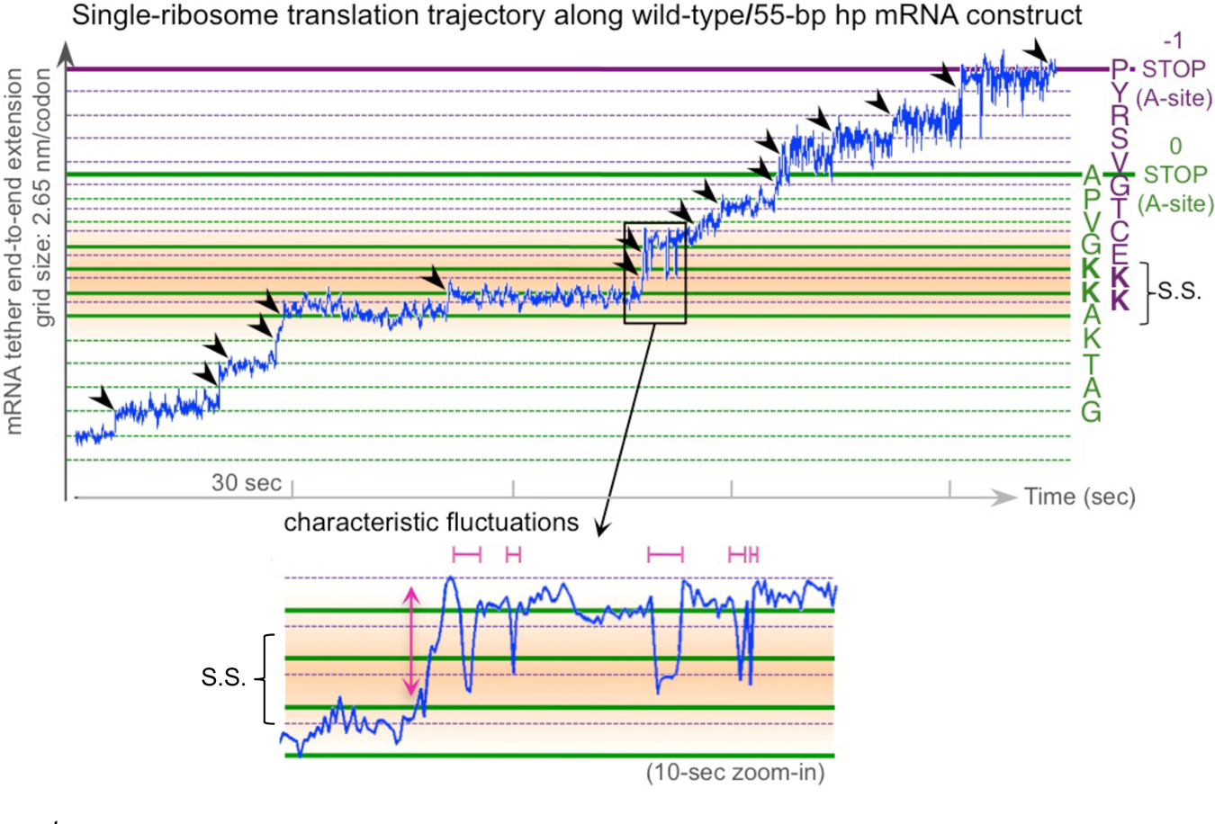
It has been shown that significant secondary structures exist in the coding regions of mRNA and that these structures can serve a regulatory purpose in process such as protein folding and frameshifting. Indeed, ribosome slowdown between protein domains can facilitate piece-wise folding of the protein (Watts et al., Reference Watts, Dang, Gorelick, Leonard, Bess, Swanstrom, Burch and Weeks2009). Also, changing the coding sequence to disrupt the secondary structure of the mRNA without altering the amino acid sequence of the product (synonymous mutations) has been shown to decrease the correctly folded faction of that protein product. These secondary structures exert these effects by functioning as a mechanical barrier to the passage of the ribosome and slowing it down. The reason is that the entry port of the mRNA in the ribosome, formed by proteins S3, S4, and S5 is too narrow to permit passage of double-stranded helical structures. Therefore, secondary structures formed in the mRNA must be disrupted before they can move through the ribosome entry tunnel.
Crystal structure (Yusupova et al., Reference Yusupova, Yusupov, Cate and Noller2001), bulk oligonucleotide displacement assays (Takyar et al., Reference Takyar, Hickerson and Noller2005), and our own optical tweezers measurements (Qu et al., Reference Qu, Wen, Lancaster, Noller, Bustamante and Tinoco2011) have shown that the distance between the first nucleotide in the peptidyl site to the mRNA entry site is 13 ± 2 (s.d.) nucleotides. Accordingly, when the ribosome translates codon i at the aminoacyl site, translocation to the next codon requires the unwinding of codon i + 4 at the entry site. The strand separation activity is inherent to the ribosome, requiring no exogenous helicases (Takyar et al., Reference Takyar, Hickerson and Noller2005) but its mechanism of operation remains a subject of active research. Moreover, to really understand the regulatory function of the secondary structures, we must establish how the stability of the secondary structure affects the rate of translation. Xiaohui Qu a joint postdoctoral associate between Nacho's laboratory and mine implemented the RNA hairpin assay to address these issues. To this end, Xiaohui used two hairpin-containing mRNAs, one with ~50% GC content and the other with 100% GC content. She found that the translation rate of identical codons at the decoding center is greatly influenced by the GC content of folded structures at the mRNA entry site. Furthermore, force applied to the ends of the hairpin significantly speeds up translation (Fig. 46). Helicases are usually classified as passive or active (Betterton and Julicher, Reference Betterton and Julicher2005). A passive helicase is one unable to separate the strands of the nucleic acid and it must await the spontaneous opening of the junction to advance. An active helicase, instead, upon contacting the junction destabilizes it by some energy amount ΔG, that favors its open state. Application of this canonical model to the data obtained by the ribosome was unable to account for the force and GC content dependence of the ribosome velocity. To fit the data, we needed to postulate that the ribosome, unlike previously studied helicases, uses two distinct active mechanisms to unwind mRNA structure: it destabilizes the helical junction at the mRNA entry site by biasing its thermal fluctuations toward the open state, increasing the probability of the ribosome translocating unhindered; and it mechanically pulls apart the RNA strands of the closed junction during the conformational changes that accompany ribosome translocation. This study was published in 2011 (Qu et al., Reference Qu, Wen, Lancaster, Noller, Bustamante and Tinoco2011).
Dependence of translation rate on force and mRNA GC content. (a) mRNA designs for 50% and 100% GC unwinding Note that given a footprint size of 13 nt from the ribosome P-site to the mRNA entry pore, when the i-th codon in the ribosome A-site (magenta) is translated, the subsequent translocation corresponds to unwinding the (i + 4)-th codon downstream (green). E, exit site; P, peptidyl site; A, aminoacyl site. (b) Translation rate dependence on force for hpValGC50 (left, ~50% GC unwinding) and hpValGC100 mRNA (right, ~100% GC unwinding). Blue circles show experimental data. Black solid, dashed, and dot–dash lines show the force dependence predicted by the Betterton model, v = vssfopen, with ΔG d = 0, 1.1, and 2.2 kcal⋅mol−1 bp−1, respectively. The black solid line represents a totally passive helicase, whereas the blue and red solid lines show the best fit following the proposed two-mode unwinding kinetic scheme (Qu, et al., Reference Qu, Wen, Lancaster, Noller, Bustamante and Tinoco2011) Error bars, s.e.m. Reprinted with permission from Qu et al. (Reference Qu, Wen, Lancaster, Noller, Bustamante and Tinoco2011).
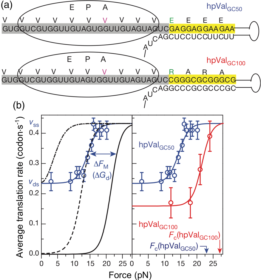
When Varsha Desai, a chemistry graduate student, joined the laboratory, she declared her interest to answer a number of questions about the translocation step in the ribosome. The first question she posed was: How do ribosomes couple their helicase activity with their translocation and how is the binding and activity of EF-G coupled to strand opening and translocation? Another way to pose this question is: When, during the cycle, are secondary structures unwound? In principle, it is possible to imagine three different scenarios: (1) hairpin opening could occur prior to EF-G binding by the positively charged amino acid residues surrounding the entry port of the mRNA tunnel (Takyar et al., Reference Takyar, Hickerson and Noller2005); (2) it could happen concomitantly with EF-G binding, using the free energy derived from binding; or (3) it could occur after EF-G binding and coinciding with the forces generated during mRNA translocation. To distinguish between these alternatives, Varsha together with postdoctoral fellows Filipp Frank and Maurizio Righini used a high-resolution optical tweezers instrument endowed with single-molecule fluorescence detection capability, or ‘fleezers’ (for fluorescence-tweezers). This instrument allowed her to monitor in a co-temporal manner both the hairpin unwinding in the optical tweezers channel, and the binding of fluorescently labeled elongation factor G (EF-G) in the fluorescence channel. The design of the experiment can be seen in Fig. 47a. As shown in Fig. 47b, hairpin opening occurs always after EF-G binding (not due to charged residues at the pore). Also, binding itself does not trigger translocation, since binding and hairpin opening do not exactly coincide. Therefore, hairpin opening is concurrent with translocation. Note that hairpin opening occurs some 250 ms after the binding of EF-G. We call this time τ unwinding. Similarly, EF-G remains bound for another 400 ms or so before detaching. We refer to this time as τ release. Next, Varsha asked which conformational changes within the ribosome result in hairpin opening? After EF-G binding, two conformational changes are known to occur in the ribosome: forward and reverse rotation of the 30S head. To decide which of these are involved in the actual opening of the hairpin, Varsha used fusidic acid, an antibiotic known to prevent the reverse rotation of the 30S head. If the forward rotation is required for hairpin opening, then we would expect τ unwinding not to change and τ release to lengthen significantly. Conversely, if reverse rotation is involved in the opening of the hairpin, we expect τ unwinding to lengthen and τ release not to change. Varsha's data showed unequivocally that the first scenario above holds, implying that the forward rotation is required for the unwinding of the mRNA secondary structures.
(a) Schematic depiction of the simultaneous optical tweezers/confocal fluorescence detection experiments. The optical trap lasers and the fluorescence laser are turned on and off according to the operational sequence: trap-1, fluorescence, trap-2, trap-1, fluorescence, trap-2, etc. so as to avoid interference between the force and fluorescence channels. Here an mRNA hairpin is held under a high external force of 13–16 pN, and the ribosome translation is supplemented with 10 nM Cy3-labeled-EF-G. (b) Top trace: movement of the ribosome is registered in the force channel, where the ribosome opens the hairpin in one-codon steps (i.e., 6-nt increment), separated by dwells, τ dwell. The data were recorded at 133 Hz and displayed at 13 Hz. The yellow box shows a magnified event. Bottom trace: arrival/binding of a Cy3-labeled EF-G (see panel A) appears as a spike in the fluorescence channel. The yellow box shows a magnified event. The data were recorded at 100 Hz and displayed at 10 Hz. The time resolution of the optical tweezers channel is 7.5 ms and 10 ms for the fluorescence channel. Right scheme: summary of average τ dwell (gray), average EF-G residence times before unwinding (τ unwinding, green), and after unwinding (τ release, green) for a weak hairpin held under an external force of 13–16 pN (n = 55 events, 9 molecules). Error bars, s.e.m. Reprinted with permission from Desai et al. (Reference Desai, Frank, Lee, Righini, Lancaster, Noller, Tinoco and Bustamante2019).
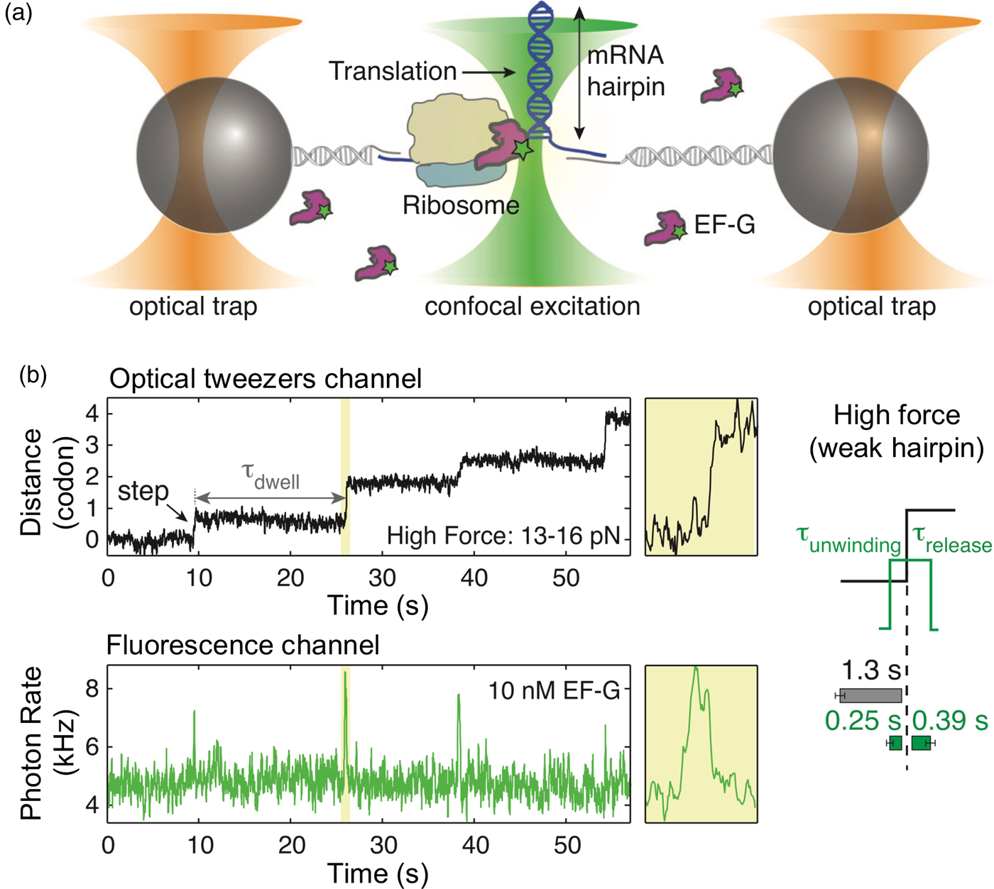
Next, Varsha asked: Do secondary structures selectively reduce the rate of the strand-opening step? Or they affect other steps in the translation cycle? To this end, Varsha revisited Xiaohui's approach of varying the force applied by the optical tweezers to the hairpin junction to increase or decrease the strength of the barrier. These experiments confirmed Xiaohui's results that the rate of translation increases with the force applied to the junction. Varsha found that decreasing the applied force increased the duration of the dwells by one full second. Surprisingly, however, she found that the increase of τ unwinding (from 250 to 560 ms) could not account for the total increase in the dwell time. Since the release time is not affected by the magnitude of the applied force, it follows that other events – after the synthesis of the peptide bond and prior to EF-G binding – are sensitive to mRNA barriers. In other words, it is as if when encountering a barrier, the ribosome changes gear and slows down not only the step involved in the opening of the junction but also prior steps of the translation cycle. Analysis of the overall cumulative dwell time distribution showed that its fitting required two exponentials:

where k slow and k fast represent two different translation rates of the ribosome that differ by a factor of 5 but that are themselves force independent. What is force dependent, instead, are the fraction time f slow and f fast that the ribosome uses the slow rate and the fast rate, respectively. A similar result is obtained for the cumulative distribution of the τ unwinding. Finally, as expected, τ release is independent of the applied force. These results reveal that in front of a weak barrier, the ribosome translocates via a fast pathway (or high gear) 90% of the time and uses a slow pathway (or low gear) only 10% of the time. In front of a strong barrier, however, the ribosome now uses the slow and the fast gear about equal time. This idea is illustrated in Fig. 48.
Ribosome translates through a hairpin via two parallel pathways that bifurcate before EF-G binding and converge after hairpin opening (Desai et al., Reference Desai, Frank, Lee, Righini, Lancaster, Noller, Tinoco and Bustamante2019). Proposed kinetic scheme: the ribosome ‘senses’ the hairpin barrier and irreversibly switches into either a fast state (green) or a slow state (red) via rates $k_{{\rm sensor}}^{{\rm fast}}$ or $k_{{\rm sensor}}^{{\rm slow}}$
 , respectively. The ratio $k_{{\rm sensor}}^{{\rm fast}} /k_{{\rm sensor}}^{{\rm slow}}$
 is force sensitive and determines the fraction (f) of translation events that go through either pathway. For example, f slow path increases from ~10% at high force (>10 pN, top scheme) to ~50% at low force (<7 pN, bottom scheme). Then, the ribosome in either the fast or the slow state must undergo an intermediate transition that becomes rate limiting at low force and determines the overall rates. It is likely that this intermediate transition is the rate of EF-G binding.
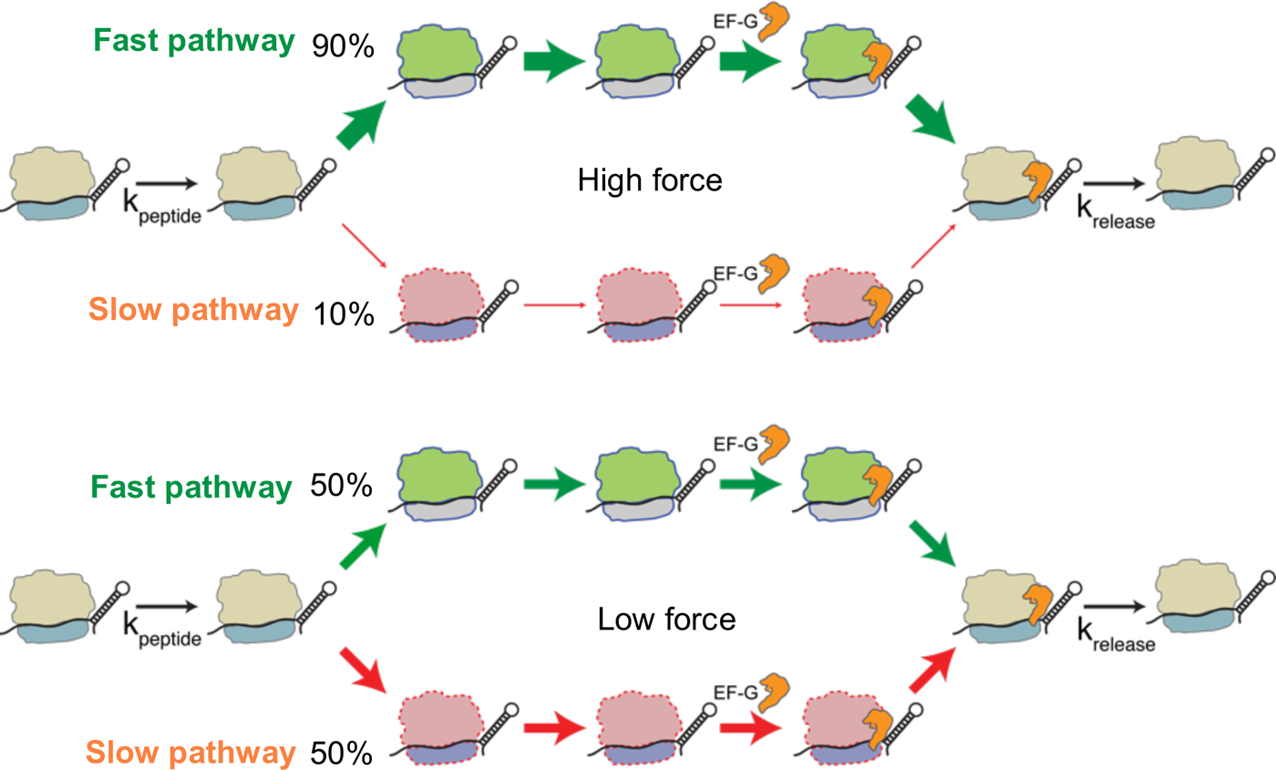
We can only speculate as to why is that the ribosome responds in this global manner to the presence of strong barriers. One possibility is that this property has evolved to exploit the presence of secondary structures in the mRNA in order to favor the slowing down of the synthesis and to favor the attainment of certain intermediate folding states of the nascent chains. It is also possible that this is a manifestation of the adaptation of molecular machines throughout evolution to improve their thermodynamic efficiency. Slowing down globally in front of a barrier would give the ribosome time to unwind the hairpin without multiple attempts, thus minimizing the use of GTP (see section ‘A final conjecture about molecular machines’ below). These findings were made possible by an excellent team work of Varsha, Filipp, Maurizio, as well as another graduate student Antony Lee, and were published in 2019 (Desai et al., Reference Desai, Frank, Lee, Righini, Lancaster, Noller, Tinoco and Bustamante2019).
A final conjecture about molecular machines
Reversible heat engines operating infinitely slowly according to a Carnot, Otto, or Stirling cycle, for example, do not dissipate energy; their energetic efficiency is limited only by the entropy increase of the surroundings associated with the transfer of heat from a hot to a cold reservoir. In contrast, for engines operating irreversibly, the extra non-equilibrium energy cost of carrying out a process at a finite rate further reduces their efficiency (Callen Reference Callen1991). This is the case of biological machines (Howard, Reference Howard2001) that must operate under cell cycle time constraints. We can then ask: what factors determine their unprecedented thermodynamic efficiency?
Sara Tafoya, in collaboration with David Sivak at the Simon Fraser University, decided to investigate the concept of ‘thermodynamic length’. Imagine a nanoscale system in contact with a thermal bath driven from one equilibrium state, A, to another, B in a finite time interval, τ, by manipulating an external parameter λ(x). What is the optimal non-equilibrium path or protocol (dλ(x)/dt) from A to B performed in the interval τ that dissipates less energy? It is possible to define a metric on the parameter space such that the amount of dissipation generated in a given path is directly proportional to the length of that path (its ‘thermodynamic length’) (Sivak and Crooks, Reference Sivak and Crooks2016). The optimal (shortest) path from A to B is then a ‘geodesic’ in parameter space. Recently, a generalized friction coefficient – which can be obtained from equilibrium measurements – was shown to be the parameter that governs the energy dissipation during finite-rate processes (Sivak and Crooks, Reference Sivak and Crooks2012). According to the theory, near equilibrium, the protocol that minimizes dissipation for a given total duration must proceed with a velocity, dλ(x)/dt, proportional to the inverse square root of the value of the local friction coefficient (Sivak and Crooks, Reference Sivak and Crooks2016). Sara confirmed experimentally this prediction using an RNA hairpin that was driven from its folded to its unfolded state using optical tweezers. She obtained the value of the generalized friction coefficient from the autocorrelation of equilibrium fluctuations of the force and showed that the protocol in which the speed of the control parameter follows that prescribed by the theory indeed minimizes the dissipation (Tafoya et al., Reference Tafoya, Large, Liu, Bustamante and Sivak2019). These results lead to a crucial and experimentally testable conjecture: ‘Have biological machines evolved to follow paths that minimize thermodynamic length during their operation, changing their speed to minimize dissipation?’. This is an intriguing question and one that is currently a subject of active research.
Future perspectives
In the three decades that have elapsed since the publication of the first direct mechanical manipulation of a DNA molecule experiment, the applications of single-molecule force spectroscopy have grown at an increased pace encompassing an ever-larger number of problems in biophysics. Their increased utilization derives from the fact that, by avoiding the averages implicit in ensemble experiments, these methods yield dynamic information in the form of ‘molecular trajectories’ that are more readily amenable to mechanistic interpretation than the signals measured in bulk. Moreover, by making force (detected or exerted) and the ensuing displacements directly measurable (from which work can be calculated), these methods afford the experimenter the unique ability to simultaneously monitor the dynamics and the energetics of a system.
The increased application of these methods has, in part, resulted from the accelerated improvement in the temporal and spatial resolution of the instruments (optical tweezers, magnetic tweezers, AFM-based actuators) employed in their execution. Furthermore, the development of hybrid instruments with simultaneous force and fluorescence spectroscopy-measuring capabilities, promises to provide a richer description of the systems of interest, by making it possible to follow the dynamics of orthogonal variables in a co-temporal fashion, from which causal relationships between those observables can be readily established.
There are still many growth opportunities lying ahead for the field of single-molecule force spectroscopy. First, a gap still exists between in vitro and in vivo experiments, and it is imperative that we attempt to close this gap. One way to do so could be to develop robust protocols to perform single-molecule experiments using cell extracts. Then, by effecting selective depletion of specific components using immuno-precipitation, or enrichment of specific components, it should be possible to establish correlations and deconstruct the response of systems in a context that resembles the cell milieu. A second opportunity arises from the fact that although force spectroscopy has revealed the importance of forces and stresses in the operation of many biological processes, we need to be able to measure those forces and stresses inside the cell and at the single-molecule level, ideally through the development of genetically encoded strategies. Although challenging, this objective is not unreachable, and its attainment will likely benefit from crucial developments in instrumentation and in experimental design.
The convergence of improved instrumentation, with the vast amount of experience gathered during the last three decades on the best protocols to perform single-molecule force spectroscopy, bodes well for the further development of these methods and their contributions to molecular biophysics.


 Open access