2.1 Equation of particle motion for inertial floating disks in the swash zone

We consider the forces acting on an inertial, floating, disk-shaped particle during a single wave swash event on an inclined slope using a framework from Reference Maxey and RileyMaxey and Riley (1983). The work from Reference Maxey and RileyMaxey and Riley (1983) has been expanded to include a free surface with regular waves by Reference Rumer, Crissman and WakeRumer, Crissman, and Wake (1979). The regular wave free surface model has been further expanded to consider the object motion to be driven by gravity (Reference Calvert, McAllister, Whittaker, Raby, Borthwick and van den BremerCalvert et al., 2021; Reference Huang, Huang and LawHuang, Huang, & Law, 2016; Reference Shen and ZhongShen & Zhong, 2001) where the particle slides down the slope of a surface wave in a reference frame that rotates with the wave motion. The work from Reference Maxey and RileyMaxey and Riley (1983) has been separately expanded to include a free surface and surface current by Reference Beron-Vera, Olascoaga and MironBeron-Vera, Olascoaga, and Miron (2019). Under bore-driven swash, the slope of the free surface is small (Reference Meyer and TaylorMeyer & Taylor, 1972), so we maintain an inertial reference frame and consider the particle motion to be driven by the swash flow current similar to Reference Beron-Vera, Olascoaga and MironBeron-Vera et al. (2019).

Figure 1(a) shows the model and experimental set-up with the piston-type wave maker, the plane, impermeable beach at an angle $\tan \theta = 1/10$, the undisturbed wave characteristics and the run-up and draw-down wave profiles. The undisturbed, floating disk-shaped particle is depicted in figure 1(b) with diameter $D_{p}$, height $H_{p}$, submerged height $H_{pw}$ and height above the water surface $H_{pa}$. Figure 1(c,d) shows the particle during run-up and draw-down, respectively. We choose a disk-shaped particle with a single aspect ratio, which can represent a range of non-idealized, but highly oblate (flattened) debris shapes that are common for plastics in the environment (Reference RosalRosal, 2021; Reference Voth and SoldatiVoth & Soldati, 2017). Additionally, the disk shape simplifies the analysis significantly compared with the sphere considered previously (Reference Beron-Vera, Olascoaga and MironBeron-Vera et al., 2019) since the submerged particle depth is linearly proportional to the volume of water displaced. We define an $x$–$z$ coordinate system whose origin is at the undisturbed shoreline with $x$ pointing horizontally towards the shore and $z$ vertically upwards. Considering only the forces on the particle from the water (and ignoring forces from the air), we formulate a particle equation of motion that considers the particle to be in vertical equilibrium and subject to forces in the horizontal direction.

Figure 1.

(a) Definition sketch of the incident wave and resulting swash flow acting on the plane beach with an oblique overhead camera. The solid line indicates the water profile during the wave run-up, the dashed line indicates the water profile during run-down and the dotted line indicates the offshore wave profile. The coordinate origin is noted where the still water surface contacts the beach. (b) The undisturbed particle floats with the submergence ratio equal to the density ratio. (c) During the wave run-up, the particle is drawn to the swash tip and remains freely floating due to the depth at the bore front. (d) During the wave draw-down, the depth of the water can decrease below the free floating $H_{pw}$, and the particle makes contact with the bottom surface.

During the wave run-up, the particle does not touch the beach (figure 1c) and remains in vertical equilibrium where the mass of the particle ($m_p$) is equal to the mass of the fluid displaced by the particle ($m_f$). Once the water depth decreases below $H_{pw}$ at equilibrium, the particle makes contact with the beach; when the particle touches the bottom (figure 1d), the mass equivalency no longer holds since there is an additional reaction force with the beach. For later use in the horizontal momentum balance, we consider the ratio of the mass of the fluid displaced to the mass of the particle

(2.1)\begin{equation} \frac{m_f}{m_p} = \frac{\rho}{\rho_p}\frac{\dfrac{\rm \pi}{4}D_p^2 H_{pw}}{\dfrac{\rm \pi}{4}D_p^2 H_p} = \frac{\phi}{\gamma}, \end{equation}

where $\rho _p$ is the particle density, $\rho$ is the fluid density, $\gamma$ is the particle to fluid density ratio and $\phi = H_{pw}/H_p$ is the particle submergence ratio. Equation (2.1) is unity when the particle weight is completely opposed by buoyancy and zero when the particle weight is completely opposed by the reaction force with the beach. Critically, $\phi = \gamma$ when the particle is floating (figure 1c), and $\phi \neq \gamma$ when the water depth is too shallow for the particle to completely float (figure 1d).

For the particle motion up the beach, we consider the acceleration in the $x$-direction, which is different to the direction up the slope of the beach by a factor of $\cos \theta$. Because the angle $\theta$ tends to be small, the difference between the horizontal and beach-parallel directions is negligible. Consider that $\cos \theta = 1- \frac {1}{2}\theta ^2 + \mathcal {O}(\theta ^4)$ and $\tan \theta = \theta + \mathcal {O}(\theta ^3)$ for small $\theta$. Using $s=\tan (\theta )$ to define the slope, we see that $\cos \theta \approx 1$ with a leading-order error of $\frac {1}{2}s^2$. For a beach slope of $s=1/10$, this leading-order error is $5 \times 10^{-3}$ and thus is negligibly small.

The swash flow drives the particle motion. Here, we employ a one-way coupled equation to model the particle motion, which is justified since the particle is small compared with the typical swash run-up lengths and the disturbance of the flow from the particle is of second-order importance (Reference Balachandar and EatonBalachandar & Eaton, 2010; Reference Maxey and RileyMaxey & Riley, 1983). The horizontal forces on the particle are due to fluid forcing, added mass, drag force and frictional force with the beach. This is expressed dimensionally as

(2.2)\begin{equation} m_p\frac{{\rm d} v'_p}{{\rm d} t'} = m_f \frac{{\rm D} u'}{{\rm D} t'} + C_m m_f \left( \frac{{\rm D} u'}{{\rm D} t'} - \frac{{\rm d} v'_p}{{\rm d} t'} \right) -C_D \frac{1}{2}\rho |v'_p - u'|(v'_p-u')D_p H_{pw} + \left[F'_F\right], \end{equation}

where $v'_p$ is the velocity of the particle, $u'$ is the fluid velocity, $C_m$ is the coefficient of added mass, $C_D$ is the coefficient of drag, $F'_F$ is the force of friction with the beach (only acting when the water depth is sufficiently small that the particle makes contact with the beach) and ${\rm D}/{\rm D} t = \partial /\partial t + u \partial / \partial x$ is the material derivative. Here, we note that the $v'_p$, $u'$, $t'$ and $F'_F$ are dimensional variables as indicated by the prime notation.

We divide (2.2) by $m_p$ using (2.1) and simplify to isolate the particle acceleration. We let the acceleration due to friction be $a_F' = F'_F/m_p$. We address the frictional acceleration fully in § 2.2. We also define a Reynolds number of the flow by the particle slip velocity and particle diameter as $Re =|v_p' - u'|D_p/\nu$. The resulting equation for the particle acceleration is

(2.3)\begin{equation} \frac{{\rm d} v'_p}{{\rm d} t'} = \left( \frac{\phi + C_m \phi}{\gamma + C_m \phi} \right) \frac{{\rm D} u'}{{\rm D} t'} - \left( \frac{1}{\gamma + C_m \phi} \right) \frac{2 C_D \phi \nu}{ {\rm \pi}D_p^2 }Re(v'_p-u') + \left[a'_F\right]. \end{equation}

The drag coefficient for a cylindrical disk is a function of $Re$. The solid, black line in figure 2 sketches this function over a range of $Re$ (Reference Clift, Grace and WeberClift, Grace, & Weber, 2013). The dotted blue line indicates the Stokes drag model, $C_D = 13.6/Re$ for a circular disk oriented such that its axis of symmetry is parallel to the flow (Reference Happel and BrennerHappel & Brenner, 1983). The Stokes model does not well represent the true value of $C_D$ in the shaded region, which is the intermediate $Re$ regime that is typical of a swash flow. Similar to Reference DiBenedetto, Clark and PujaraDiBenedetto, Clark, and Pujara (2022), we approximate $C_D$ in the intermediate $Re$ regime as inversely proportional to $Re$ with a new, unknown proportionality constant, $C$, noted by the dashed red line in figure 2. We substitute $C_D$ for the intermediate $Re$ regime into (2.3) to get

(2.4)\begin{equation} \frac{{\rm d} v'_p}{{\rm d} t'} = \beta \frac{{\rm D} u'}{{\rm D} t'} - \frac{(v'_p-u')}{\tau_p} + \left[a'_F\right], \end{equation}

where

(2.5a,b)\begin{equation} \beta = \frac{\phi + C_m \phi}{\gamma + C_m \phi}; \quad \tau_p = \frac{{\rm \pi} D_p^2 (\gamma + C_m \phi)}{2 C \phi \nu}. \end{equation}

Here, $\beta$ represents the strength of the fluid forcing and added mass of the fluid acting on the particle, and $\tau _p$ represents the relaxation time for the particle in the flow. The unknown empirical coefficient in the drag formulation, $C$, is absorbed into the particle time scale. We also note that when the water is deep enough such that the particle is freely floating, we can show that $\beta = 1$ from (2.1).

Figure 2.

The black line indicates the coefficient of drag as a function of the Reynolds number for a particular shape. The blue dotted line is the Stokes drag approximation for low $Re$ and the red dashed line is the intermediate $Re$ approximation.

In a swash flow event, the relevant scales of motion are the initial shoreline velocity ($U_s$) and gravity ($g$). Using these scales to make (2.4) dimensionless, we define the dimensionless variables $u = u'/U_s$, $v_p = v_p'/U_s$, $t = t'/(U_s/g)$ and $a_F = a_F'/g$. This gives

(2.6)\begin{equation} \frac{{\rm d} v_p}{{\rm d} t} = \beta \frac{{\rm D} u}{{\rm D} t} + \frac{(u - v_p)}{St} + \left[a_F\right], \end{equation}

where the particle Stokes number is given by

(2.7)\begin{equation} St = \frac{g \tau_p}{U_s}. \end{equation}

In (2.6), the fluid forcing and the added mass force are captured in the first term, and the drag of the fluid on the particle is captured in the second term.

In addition to the equation for particle motion, we use a classical model for swash flow (Reference Peregrine and WilliamsPeregrine & Williams, 2001; Reference Shen and MeyerShen & Meyer, 1963). For a given beach slope $s$, the shoreline position, shoreline velocity, flow velocity field and water depth are given by

(2.8a)$$\begin{gather} x_s = t - \frac{1}{2}st^2, \end{gather}$$

(2.8b)$$\begin{gather}u_s = 1 - st, \end{gather}$$

(2.8c)$$\begin{gather}u = \frac{1}{3} \left(1-2st + 2\frac{x}{t}\right), \end{gather}$$

(2.8d)$$\begin{gather}h = \frac{1}{9} \Bigl(1-\frac{1}{2}st - \frac{x}{t} \Bigr) ^2, \end{gather}$$

where $x_s = x_s'/(U_s^2/g)$ is the dimensionless shoreline position, $u_s = u_s'/U_s$ is the dimensionless shoreline velocity, $u = u'/U_s$ is the dimensionless fluid velocity and $h = h'/(U_s^2/g)$ is the dimensionless water depth. This bore-driven swash model has been shown to accurately describe the flow evolution in a single swash event in laboratory experiments (see figures 19–20 corresponding to surging and plunging breaker in Reference Pujara, Liu and YehPujara et al., 2015). Thus, the model of swash flow accurately captures the flow evolution in a swash event, but does not necessarily account for other complexities in the swash zone such as infragravity waves or swash interaction between waves.

2.2 Extra considerations for beaching particles

We supplement (2.6) to capture aspects of particle motion in the swash zone that are critical, but not included in the dynamics so far. Specifically, we account for the dynamics of the swash tip where debris particles will collect. We also consider the frictional force on the particle with the beach when the water depth goes to zero.

The swash tip is typically a blunt edge (figure1c) due to the effects of friction and flow convergence (Reference Baldock, Grayson, Torr and PowerBaldock, Grayson, Torr, & Power, 2014; Reference Pujara, Liu and YehPujara, Liu, & Yeh, 2016), which will collect debris particles during the wave run-up. However, this is not captured in the flow model. To account for particle motion in the swash tip, we first define the particle location ($x_p$) relative to the shoreline location ($x_s$) as

(2.9)\begin{equation} \xi = x_s - x_p. \end{equation}

We then make two modifications to the swash model. The first is that during the run-up, we expect the depth of the water near the swash tip to be greater than the particle since friction creates a ‘blunt nose’ at the tip. Using the definition of $\beta$ from (2.5a,b), we make the simplification that $\beta =1$ throughout the wave run-up. Second, we implement a spatial dependency on the Stokes number during the run-up, which accounts for the fact that the particle becomes more tracer-like in the fast and turbulent swash tip

(2.10)\begin{equation} St_{eff} = C_{St} St = \frac{1}{1 + \exp({-k(\xi-w)})} St. \end{equation}

Here, the coefficient $C_{St}$ ranges from 0 to 1, acting to decrease the effective Stokes number in the vicinity near the tip during the wave run-up, which is essentially a boundary layer to the swash flow. The constant $k$ represents a sharpness factor that determines how smoothly the $C_{St}$ varies with $\xi$, and $w$ determines the width of the zone where the $C_{St}$ noticeably falls below unity. While the results presented below are not sensitive to the precise values, using $k = 10$ and $w = 0.25$ provides an effective region of approximately 1/10 of the maximum run-up where the Stokes number is modified (figure 3). The swash tip size ($10\,\%$ of the maximum run-up) is an approximation, but consistent with previous data and models of the swash tip (Reference Baldock, Grayson, Torr and PowerBaldock et al., 2014; Reference Pujara, Liu and YehPujara et al., 2016).

Figure 3.

The Stokes number coefficient ($C_{St}$) during the wave run-up, shown as a function of the particle position relative to the shoreline ($\xi$) and the shoreline position ($x_s$); $C_{St}$ decreases for a particle near the shoreline, while a particle far from the shoreline is unaffected. The Stokes coefficient noticeably deviates from unity in the region of approximately 1/10 of the maximum run-up.

On the wave draw-down, we consider the particle to be prone to beaching if it is left behind by the fluid and the local water depth at the particle becomes zero. In reality, the particle will make contact with the beach and the solid body friction force will be non-zero before the beach is completely dry (figure 1d). However, we assume that the flow dynamics will be more important than the lubricated friction force until the water depth reaches zero and as such can be neglected. Once the local water depth at the particle goes to zero, there is no buoyant force on the particle and the particle's weight is only balanced by the reaction force from the beach. In the $x$-direction, there is no longer any force from the fluid and the only force on the particle is the friction force acting opposite to its direction of motion. We model this friction force using the standard formulation $F_F = \mu N = \mu m_p g$, where $\mu$ is the coefficient of friction between the particle and the beach. In the absence of water, the deceleration of the particle due to friction is then given by

(2.11)\begin{equation} a_F = {-} \mu \operatorname{sgn}{}(v_p). \end{equation}

2.3 Model results

We solve the full model, (2.6) with the spatially dependent Stokes number (2.10) and the optional friction acceleration term (2.11) with MATLAB using a standard solver (ode45). The model parameters including $\gamma$, $C_m$, $\mu$ and $H_p$ are chosen for the case of the experimental particles in § 3. The particle begins moving at $(x, t) = (0,t_{p0})$ with an initial velocity $v(x=0,t=t_{p0}) = V_{p0}$. Initializing the model in this way also serves to avoid the singularity in the flow velocity, depth and acceleration which are undefined at $(x=0,t=0)$.

We show the impact of particle inertia and initial conditions on the beaching dynamics in figure 4. The figure shows the final location of the particle at the given conditions. After a particle is returned to the water, the model is no longer accurate and the final location is left blank as the particle is not deposited on the beach. We consider Stokes numbers in the range $St \in [1,10]$, which is a realistic range considering that it covers $\tau _p \in [0.2, 2]$ s for a swash event with $U_s = 2$ m s$^{-1}$. For the particle's initial velocity, we consider the range $V_{p0}/U_s \in [0.5, 1]$. While the lower limit is an arbitrary choice, the upper limit corresponds physically to a particle that is caught in the bore front. Apart from the initial velocity, the initial time at which the particle enters the swash zone is also important. The initial dimensionless time of the particle crossing $x=0$, $t_{p0}/(2U_s/(gs)) = [0.001, 0.01, 0.1]$ relates to the distance the particle is behind the swash tip at the start of the run-up. For the smaller dimensionless zero-crossing time, the particle is closer to the bore front.

Figure 4.

Fraction of final particle location over maximum shoreline run-up, for beaching particles as a function of particle Stokes number ($St$) and dimensionless initial particle velocity ($V_{p}/U_s$) at three dimensionless initial particle times: (a) $t_{p0}/(2U_s/(gs)) = 0.001$, (b) $t_{p0}/(2U_s/(gs)) = 0.01$, (c) $t_{p0}/(2U_s/(gs)) = 0.1$, where $2U_s/(gs)$ is the duration of the swash event. The dotted and dashed white lines indicate transects considered in figure 5.

Although we treat them separately in figure 4, we note that the initial particle velocity and time are likely to be correlated such that a particle that enters the swash later is likely to do so at a lower velocity. Additionally, we expect the particle $St$ and the initial conditions to be related as the particle inertia likely dictates motion in the surf zone and thus the resulting initial conditions.

As expected, the likelihood of particle beaching increases at higher $St$. This is because at higher $St$, the particle does not change direction as quickly as the water. The water drains before the particle can respond, leaving the particle beached. We also observe that particles are more likely to beach when they enter the swash zone at a higher initial velocity. The larger initial velocity causes the particle to stay near the swash tip, reach closer to the maximum wave run-up, and become deposited on the beach during the downrush. When a particle enters the swash close behind the swash tip, we see that it is very likely to be beached (figure 4a). In this case, the beaching location is also very sensitive to $St$. When a particle enters the swash far behind the swash tip, it is far less likely to be beached (figure 4c). The particle will only beach in this case if it is very inertial and has a large initial velocity. Under the intermediate initial time (figure 4b) beaching depends on both $St$ and the initial particle velocity, which we explore further in figure 5.

Figure 5.

Model particle trajectories at transects from figure 4 with one varied parameter. (a) Transect at the vertical dotted line in figure 4(b) showing varied $St$. (b) Transect at the horizontal dashed line in figure 4(b) showing varied dimensionless velocity.

Figure 5(a) shows the particle trajectories from figure 4(b) with $V_{p0}/U_s = 0.75$ and varied $St$. We see that, across this range of $St$, the particle trajectory and final particle location change significantly. Similarly, figure 5(b) shows the particle trajectories from figure 4(b) with $St = 5$ with varied initial particle velocities. We again see that the particle trajectory and resultant beaching location change significantly. Overall, whether a particle is beached and the location where it is beached is quite sensitive to the particle's swash Stokes number and its initial conditions as it enters the swash.

3.1 Wave flume experiments

We performed particle beaching experiments in the Water Science and Engineering Laboratory wave flume at the University of Wisconsin - Madison. The wave flume is 39 m long, 0.91 m wide and 1.12 m tall. We use a piston-type wave maker to generate a solitary wave (Reference GoringGoring, 1978) that acts incident to a 1/10 sloped impermeable, plane beach shown in figure 1(a). The generated wave has an amplitude of 0.06 m at the still water depth of 0.3 m ($a/h = 0.2$). This wave incident on the specified beach produces a surging-type breaking wave (Reference Grilli, Svendsen and SubramanyaGrilli, Svendsen, & Subramanya, 1997).

We place five, three-dimensionally printed polypropylene plastic disks just offshore of the beach, near the still water line. The particles have measured diameters of $2.261 \pm 0.002$ cm, heights of $0.268 \pm 0.003$ cm and masses of $0.819 \pm 0.002$ g. The average density is $0.760 \pm 0.008$ g cm$^{-3}$.

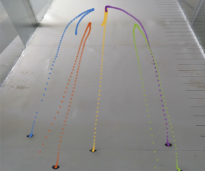
We use an obliquely mounted overhead digital camera with a frame rate of 30 f.p.s. to capture the swash event and particle motion. Throughout the camera field of view (figure 6), are calibration marks which are used to convert the particle location in pixels to distance in laboratory coordinates. We track the particle trajectories and shoreline motion using custom code written in MATLAB. For particle tracking, we first subtract the image background and binarize the image data based on a threshold that selects the particle. We manually identify the starting location of each particle and for frames after the initial two frames, we find the particle velocity from the particle displacement over the previous two frames to predict the subsequent location of the particle. We use the nearest neighbour algorithm from the predicted location to find the true location of the particle. Figure 6(a) shows the last frame with the trajectory of each particle superimposed.

Figure 6.

Oblique camera images. (a) Last frame with particle trajectories: particle A, blue squares; particle B, orange diamonds; particle C, yellow stars; particle D, purple circles; and particle E, green diamonds. (b) Sample frame during run-up. (c) Sample frame near maximum run-up.

From the camera images, we also track the shoreline position which is clearly observed by the sharp wet/dry boundary of the wavefront moving up the beach seen in figure 6(b,c). We manually track the shoreline motion during the uprush by selecting the maximum run-up location in each frame.

At the very start of the swash cycle, the shoreline motion is obstructed from view by the steepness of the breaking wave as it collapses while passing through $x=0$. We trim the data to only consider the shoreline motion after the wave bore collapsed and the position of the shoreline could be accurately tracked. However, trimming the shoreline position data means we do not know the time at which the shoreline first moved nor its initial velocity, both of which are needed for the swash model. This uncertainty is also related to the physics of bore collapse. The swash solution in (2.8) is based upon the nonlinear shallow water equations, in which the shoreline moves impulsively upon the wave bore arrival at the initial shoreline position. In reality, the wave bore collapse process occurs over some finite time and distance (Reference Pujara, Liu and YehPujara et al., 2015; Reference Yeh and GhazaliYeh & Ghazali, 1988). Since the bore collapse is not instantaneous, there is a brief time of shoreline acceleration before a maximum initial shoreline velocity is reached.

From the shoreline position data, we find the shoreline velocity using a Gaussian convolution (Reference Mordant, Crawford and BodenschatzMordant, Crawford, & Bodenschatz, 2004; Reference Ouellette, Xu and BodenschatzOuellette, Xu, & Bodenschatz, 2006) with a filter width of 2 frames and filter support of 7 frames. In our data, we confirm that the maximum observed shoreline velocity occurs at the same time that the wave bore visually appeared completely collapsed. Since we expect the shoreline position after complete bore collapse to follow (2.8a) (at least in the absence of friction), and $t=0$ is defined as the time at which the wave passes through $x=0$, we implement a time shift in the shoreline data to account for the finite time of the bore collapse process

(3.1)\begin{equation} x_{s,{data}} = U_s(t-t_0) - \tfrac{1}{2}gs(t-t_0)^2. \end{equation}

By fitting a portion of the data from the beginning of the wave run-up after bore collapse to (3.1) using the maximum velocity after the bore collapse as an initial guess for the initial shoreline velocity, we find the initial shoreline velocity to be $U_s = 1.89$ m s$^{-1}$. The shoreline data and model are plotted together in figure 7, where we see that the shoreline model fits the shoreline data well at the start of the uprush. The model predicts a slightly higher maximum run-up than we see in the experimental data, as expected since the shoreline model is frictionless. We do not have experimental shoreline position data during the draw-down because tracking the shoreline location optically becomes near impossible during the draw-down process when there is no longer an obvious demarcation between the dry and wet beach.

Figure 7.

Run-up shoreline data and model fit to (3.1) with an initial shoreline velocity of $U_s = 1.89$ m s$^{-1}$ and a time shift of $t_0 = 0.11$ s.

The particle data are defined on the same time vector as the shifted shoreline data. To find the exact time and velocity with which each particle crossed the initial shoreline position, $t_{p0}$ and $V_{p0}$, we fit a fifth-order polynomial to each particle trajectory and analytically evaluate the zero-crossing time and velocity.

3.2 Experimental particle trajectories and comparison with model

In figure 8 we show the experimental particle and shoreline trajectories with the model particle and shoreline trajectories. Table 1 lists the initial conditions and fate for each particle. The correlation between the particle initial velocity and initial time are shown in figure 9. Generally, a particle that enters the swash zone closer to the wavefront will enter with a greater velocity; a particle that enters the swash zone further behind the wave bore will enter with a lower velocity. Besides the particle initial conditions, the rest of the model parameters are: $\tau _p = 1$ s (corresponding to $St = 5.18$), $\gamma = 0.76$ g cm$^{-3}$, $C_m = 0.75$, $\mu = 0.15$ and $H_p = 0.268$ cm. We choose $\tau _p$ as a reasonable order of magnitude estimate of the particle time scale that facilitates agreement between the model and data. The values of $\gamma$ and $H_p$ are as measured from the experimental particles, and $C_m$ is taken as the average value between the added mass coefficient of a sphere ($C_m = 1/2$) and a circular cylinder ($C_m = 1$) (Reference NewmanNewman, 2017). The dynamic friction coefficient for non-metals usually ranges from 0.3 to 0.4 and is lower when moist or well lubricated (Reference RabinowiczRabinowicz, 1965). From the wetness of the beach surface after a swash event, we justify the estimated friction coefficient of $\mu = 0.15$. We further explore the sensitivity of the model to these predicted values in § 4.

Figure 8.

Model and experimental shoreline run-up plotted with model and experimental particle trajectory for five experimental particles with initial conditions listed in table 1. Panels (a–e) correspond to particles A–E, respectively.

Table 1.

Experimental particle initial conditions and fate from figure 8.

Figure 9.

Particle initial velocity vs. initial time. Particles that enter the swash zone closer to the wave will enter with a larger velocity, and those that are further behind the wavefront will enter the swash zone with a lower velocity.

The comparison between the data and model trajectories in figure 8 shows that the model captures the qualitative behaviour observed in the experiments. In particular, the model trajectories correctly predict whether a particle is deposited on the beach (particles A, C and D) or returned to the water (particles B and E) without any case-specific tuning of parameters. Of the beached particles, the location of beaching in the model is also close to the observed value in two of the three beaching particle cases (particles C and D). In each case, the experimental particle trajectories match the model very well at the start of the swash event, with the deviation between the data and the model growing until the time of the maximum run-up.

The shoreline evolves during run-up and does not maintain a uniform alongshore profile. We see at the maximum shoreline run-up, figure 6(c), that the shoreline is further at the spanwise centre of the beach. In addition to the shoreline evolution, we note that in figure 6(a), the particles closer to the edge drift inwards toward the centre of the beach during the run-up. This is especially evident in particles A, D and E. This drift towards the centre in combination with the non-uniform shoreline profile means that the particles starting at the edges fall further behind the shoreline over time than is accounted for in the model. This phenomenon explains the discrepancy between the beaching locations in the experiments and in the model for particle A.

In figure 8, for particles B–E, the particle trajectory model and data match well during the first third of the swash cycle, but start to deviate near the peak of the trajectory. Given that we have made no attempt to fine tune the particle Stokes number, which is based on an order of magnitude estimate of the particle time scale ($\tau _p = 1$ s), the model can be considered quite robust in terms of capturing the essential particle motion and fate. However, this does point to a need to better understand particle inertia for debris in the swash zone.

Apart from considering the particle trajectories between the model and experiment, another useful comparison is examining the particle trajectory relative to the shoreline, in the experiment and the model. This captures whether the model contains enough physics to predict the particle beaching dynamics. In this regard, we see that the trends of particle behaviour with the shoreline compare very well for all three beaching particles in the experiment and the model. Not only do the model trajectories capture the particle deceleration during uprush that is the result of the complex flow–particle interaction, but they also capture how the particle decelerates to zero velocity as it gets beached. Further, the experimental results confirm the fact that beaching was very sensitive to initial conditions which is consistent with the model results (§ 2.3).

Finally, we consider the acceleration budget of particles A, B and C, in figure 10. Two of these are beaching particles (particle A, deposited high on the beach in the model, and particle C, deposited lower on the beach in the model), and one returns to the water (particle B). At the beginning of each particle's trajectory, each particle experiences a positive (up the beach) force from the first term in (2.6) and a greater force acting in the opposite, negative (down the beach) direction from the middle term of (2.6). For the particles that eventually beach, these two forces both quickly approach zero during the uprush; this occurs faster for particle A (figure 10a) which is beached close to the maximum run-up. For the particle that returns to the water (particle B, figure 10b), the first and second terms decrease in magnitude slower. After the flow reverses direction at the particle location, noted by the vertical black dashed line, the second term (drag) increases in magnitude. The increased drag force is in the negative direction acting to wash the particle back into the water. We see this slightly in particle C (figure 10c), but the particle runs out of water before it travels sufficiently downslope to return to the main water body, resulting in particle beaching.

Figure 10.

Acceleration components actively contributing to the particle force balance as a function of time for particles A–C from figure 8(a–c), respectively. The dashed black line indicates the point in time where the fluid at the particle location changes direction. We note that there is a small pink region in (a), none in (b) and a larger pink region in (c).