


1. INTRODUCTION
The Greenland ice sheet (GrIS) is losing mass from increased surface melting and ice discharge from marine-terminating outlet glaciers (e.g. Sasgen and others, Reference Sasgen2012; Andersen and others, Reference Andersen2015). Ice, cloud and land elevation satellite (ICESat) missions from 2003 to 2009 revealed widespread ice thinning along the coast of the GrIS, demonstrating that the thinning rate was not uniformly distributed in space and time (Pritchard and others, Reference Pritchard, Arthern, Vaughan and Edwards2009; Sørensen and others, Reference Sørensen2011; Khan and others, Reference Khan2014). In particular, rapid thinning has been reported for fast flowing outlet glaciers (e.g. Thomas, Reference Thomas2004; Howat and others, Reference Howat, Joughin, Tulaczyk and Gogineni2005; Joughin and others, Reference Joughin2008; Motyka and others, Reference Motyka, Fahnestock and Truffer2010; Van der Veen and others, Reference Van der Veen, Plummer and Stearns2011; Kjeldsen and others, Reference Kjeldsen2013). Ice speed has increased in GrIS outlet glaciers, resulting in thinning due to longitudinal stretching, known as dynamic thinning (e.g. Pritchard and others, Reference Pritchard, Arthern, Vaughan and Edwards2009). For example, dynamic thinning accounted for ~80% of the total ice mass loss from Upernavik Isstrøm in western Greenland over the period spanning 1985–2010 (Khan and others, Reference Khan2013). The contribution of surface melting to the mass loss from GrIS outlet glaciers is also increasing as a result of recent atmospheric warming trends. Van As (Reference Van As2011) reported that surface melting on Upernavik Isstrøm has roughly doubled since the 1980s under the influence of atmospheric warming. Therefore, it is important to accurately quantify dynamic thinning and negative surface mass balance (SMB) in order to evaluate ongoing as well as future mass loss of marine-terminating outlet glaciers in Greenland. Nonetheless, the contributions of these two processes to glacier thinning are poorly understood for the majority of the rapidly changing glaciers (Howat and others, Reference Howat, Joughin and Scambos2007; van den Broeke and others, Reference van den Broeke2009).
To compute dynamically-induced ice thickness changes, it is necessary to measure ice velocity and ice thickness. Ice velocity measurements were carried out using various remote-sensing techniques, including feature tracking of orthorectified optical images (e.g. Howat and others, Reference Howat, Joughin, Tulaczyk and Gogineni2005) and interferometric synthetic aperture radar (InSAR) speckle tracking (e.g. Joughin and others, Reference Joughin, Smith, Howat, Scambos and Moon2010). Compared with velocity, ice thickness is more difficult to measure and data are sparse for most of the outlet glaciers. The quality of GrIS bed elevation maps is improving (Bamber and others, Reference Bamber2013; Lindbäck and others, Reference Lindbäck2014). For example, airborne ice radar and satellite-derived ice motion data are combined to compute precise GrIS bed topography based on mass conservation (Morlighem and others, 2013). However, resolution of the bed topography data is still insufficient to resolve detail in many outlet glaciers. Therefore, calculating dynamic thinning from velocity and thickness is limited to just a few glaciers. The magnitude of dynamic thinning was estimated by subtracting the SMB computed by regional climate models from observed elevation changes (Kjær and others, Reference Kjær2012; Khan and others, Reference Khan2013, Reference Khan2014; Kjeldsen and others, Reference Kjeldsen2013; Csatho and others, Reference Csatho2014). However, uncertainty in the computed SMB is still significant (Khan and others, Reference Khan2015), which influences the accuracy of estimates of the dynamically-induced ice thickness change. Comparing marine- and land-terminating glaciers in the same region also provides information on the importance of ice dynamics in glacier thinning. This method was applied to adjacent lake-calving and land-terminating glaciers in Alaska, and the result showed that the lake-calving glacier experienced a ~27% greater mass loss than the land-terminating glacier (Trüssel and others, Reference Trüssel, Motyka, Truffer and Larsen2013). Such a comparison has never been performed before for outlet glaciers in Greenland.
Widespread thinning of marine-terminating outlet glaciers in Greenland has been revealed by comparing elevations with repeated laser altimetry measurements (e.g. Zwally and others, Reference Zwally2011; Kjeldsen and others, Reference Kjeldsen2013; Khan and others, Reference Khan2014). Photogrammetric analysis of stereo-pair aerial photographs is another powerful tool to generate DEMs and measure elevation change (e.g. Motyka and others, Reference Motyka, Fahnestock and Truffer2010; Kjær and others, Reference Kjær2012; Khan and others, Reference Khan2013; Kjeldsen and others, Reference Kjeldsen2015). This method provides accurate measurements in the vertical and horizontal directions owing to the high-spatial resolution of aerial photographs (e.g. Kjær and others, Reference Kjær2012). Because spatial coverage is limited (<100 km2) (e.g. Kjær and others, Reference Kjær2012), a large number of photographs are required to cover the large area. One solution for achieving this high-spatial resolution plus large spatial coverage is to use satellite images for the photogrammetric analysis. Panchromatic Remote-sensing Instrument for Stereo Mapping (PRISM) images from the Advanced Land Observing Satellite (ALOS) have a spatial resolution of 2.5 m, which is sufficient to measure several metres of glacial elevation change (Sawagaki and others, Reference Sawagaki, Lamsal, Byers and Watanabe2012). The relatively large spatial coverage provided by these images (1225 km2) is suitable for studying large glaciers. DEMs derived from ALOS PRISM images were used in glacier studies in the Himalayas (Lamsal and others, Reference Lamsal, Sawagaki and Watanabe2011), Patagonia (Sakakibara and others, Reference Sakakibara, Sugiyama, Sawagaki, Marinsek and Skvarca2013; Minowa and others, Reference Minowa, Sugiyama, Sakakibara and Sawagaki2015) and Antarctica (Fukuda and others, Reference Fukuda, Sugiyama, Sawagaki and Nakamura2014), but this is the first application for marine-terminating outlet glaciers in Greenland.
As a part of a research project focused on ice mass change in the Qaanaaq region of northwestern Greenland (Sugiyama and others, Reference Sugiyama2014, Reference Sugiyama, Sakakibara, Tsutaki, Maruyama and Sawagaki2015), we carried out satellite-based observations on the marine-terminating Bowdoin Glacier and the adjacent land-terminating Tugto Glacier (Fig. 1c). Ice mass loss has increased in northwestern Greenland since 2005 (Khan and others, Reference Khan, Wahr, Bevis, Velicogna and Kendrick2010; Kjær and others, Reference Kjær2012), but few studies have been carried out in this region, compared with southern Greenland. It is crucial to study tidewater glaciers in this region in order to understand the mechanisms behind the recent increase in mass loss. We carried out additional field measurements in the lower part of Bowdoin Glacier in order to calibrate remote sensing data as well as to obtain the most recent data possible. Use of the field data for calibration is particularly important for the photogrammetric analysis of ALOS PRISM images. Bowdoin Glacier was selected as the study site because of its recent rapid retreat and acceleration (Sugiyama and others, Reference Sugiyama, Sakakibara, Tsutaki, Maruyama and Sawagaki2015). The glacier is also suitable for field measurements because of its relatively safe ice-surface conditions and proximity to Qaanaaq Airport. The aim of this study was to measure surface elevation changes on the marine- and land-terminating outlet glaciers situated in similar climate conditions. The results are compared to better understand the role of the ice dynamics in the context of the recent rapid changes of the marine-terminating Bowdoin Glacier.
(a) The location of the Qaanaaq region in Greenland. The box indicates the area shown in (b). (b) Landsat 8 OLI image (11 July 2015) showing northwestern Greenland including the studied region. The locations of Heilprin, Tracy, Melville, Hubbard, Verhoeff and Morris Jesup Glaciers are indicated as He, Tr, Me, Hu, Ve and Mo, respectively. The box indicates the area shown in (c). (c) ALOS PRISM image (4 September 2010) showing Bowdoin and Tugto Glaciers. The red dots show the locations of SMB measurements. The box indicates the area shown in (d). The contours indicate surface elevation with intervals of 100 m, based on the ALOS DEM on 4 September 2010. (d) ALOS PRISM image (4 September 2010) showing the region near the calving front of Bowdoin Glacier. GPS survey tracks are indicated on the glacier (L and T1–T3) (7–11 July 2013) and ice-free terrain (18 July 2014). The locations of SMB measurements (red dots) and the GPS reference (yellow dot) are indicated. The contours indicate surface elevation on 4 September 2010 with intervals of 20 m.

2. STUDY SITE
Bowdoin Glacier is a marine-terminating outlet glacier in northwestern Greenland, located 30 km northeast from Qaanaaq (77°41′N, 68°35′W) (Fig. 1b). Approximately 20 km long fast flowing ice bifurcates into Bowdoin Glacier and land-terminating Tugto Glacier ~10 km from the ocean (Fig. 1c). Bowdoin Glacier flows southward and discharges ice into Bowdoin Fjord through a 3 km-wide calving front at a rate of ~440 m a−1 in 2013 (Sugiyama and others, Reference Sugiyama, Sakakibara, Tsutaki, Maruyama and Sawagaki2015). Sugiyama and others (Reference Sugiyama, Sakakibara, Tsutaki, Maruyama and Sawagaki2015) report changes in the terminus position, ice thickness and ice/ocean bed geometry based on combined field and satellite observations. The terminus position had been stable since 1987, with the glacier beginning a rapid retreat in 2008. The retreat distance from 2008 to 2013 was 2 km at the western margin. Ice thickness along the glacier centre is 250–400 m within 6 km of the terminus. The glacier terminus was grounded, with 86–89% of the entire ice thickness below sea level.
Tugto Glacier flows parallel to Bowdoin Glacier, and these two glaciers are separated by a mountain ridge, by a distance of several kilometres (Fig. 1c). Tugto Glacier is ~4 km wide and the ice diverges towards the ice front, terminating on land. A part of the frontal margin touches the terminus of Qaqortaq Glacier, an outlet glacier from Qaanaaq Ice Cap (Takeuchi and others, Reference Takeuchi, Nagatsuka, Uetake and Shimada2014).
The mean annual temperature in the region is −8°C at sea level (Sugiyama and others, Reference Sugiyama2014). Bowdoin Fjord is typically covered with sea ice until early July. Air and sea surface temperatures show a warming trend in this region since the late 1990s (Sugiyama and others, Reference Sugiyama, Sakakibara, Tsutaki, Maruyama and Sawagaki2015). In July 2013–15, we performed field observations on the lower 5 km of Bowdoin Glacier (Fig. 1d).
3. DATA AND METHODS
3.1. GPS survey
The surface elevation of Bowdoin Glacier was surveyed in the field from 7–11 July 2013. We used dual frequency GPS receivers and antennae (Leica System 1200 and GNSS GEM-1) to measure 3-D coordinates of the glacier surface. One of the receivers was situated on a stable boulder on the eastern flank of the glacier as a reference station (Fig. 1d). On the glacier, more than 700 locations were surveyed by moving with a rover receiver within a region 3.3 km from the glacier terminus. These measurements were made along a longitudinal profile (L) and three transverse profiles (T1–T3) (Fig. 1d; Table 1). GPS data recorded at a sampling rate of 1 s were post-processed in kinematic mode with GPS software (RTKLIB). We processed L1 and L2 frequency data filtered with a 15° elevation mask, by correcting ionospheric and tropospheric effects. The accuracy of a kinematic GPS survey with a baseline length of 0.7–3.9 km is expected to be several centimetres in the horizontal and <0.1 m in the vertical directions. Uncertainty in the vertical position of the rover GPS antenna, which was fixed on a backpack of a surveyor, was <0.1 m. Accordingly, the total uncertainty in the vertical direction was <0.2 m, which is <10% of observed elevation changes described later in the text. Data were excluded in the event that an error estimated by the GPS software exceeded 1 m.
Date, number of points and altitude range of GPS survey on Bowdoin Glacier and ice-free terrain

To calibrate DEMs described in the next subsection, additional GPS measurements were performed outside the glacier near the eastern margin (Fig. 1d; Table 1). This survey was carried out on 18 July 2014 over an ice-free area of 5.9 km2. Relatively flat terrain (<30°) was surveyed for this purpose in order to avoid the relatively large error rate seen in steep terrain (Berthier and others, Reference Berthier2007; Fujita and others, Reference Fujita, Suzuki, Nuimura and Sakai2008; Nuimura and others, Reference Nuimura, Fujita, Yamaguchi and Sharma2012). The survey data were interpolated using the inverse distance weighting method to generate a 15 m resolution DEM (GPS-DEM); the method previously employed by Nuimura and others (Reference Nuimura, Fujita, Yamaguchi and Sharma2012) to compare GPS data and satellite-derived DEMs.
3.2. Generation of a DEM from satellite data
We generated DEMs using ALOS PRISM images (2.5 m resolution) acquired on 20 August 2007 and 4 September 2010. The DEMs cover the surface of Bowdoin and Tugto Glaciers over a 294.8 km2 area within 17 km of the terminus. We processed 1B2 level stereo pair images with digital photogrammetry software Leica Photogrammetric Suite 2011 (LPS) mounted on an ERDAS IMAGINE 2011 workstation. The images were geometrically registered based on the parameters described in rational polynomial coefficient (RPC) files. A non-uniformly distributed surface elevation dataset (triangulated irregular network: TIN) was generated using an automated routine in the LPS. To improve accuracy, the automatically generated elevation data were manually corrected by viewing stereoscopic glacier images on a stereo monitor (PLANAR SD 2020 Stereo Mirror™/3-D Monitor) (Lamsal and others, Reference Lamsal, Sawagaki and Watanabe2011). A 3-D mouse was used for this procedure (Leica 3-D TopoMouse). DEMs for 2007 and 2010 were then generated by interpolating the non-uniformly distributed elevation data with a 15 m resolution.
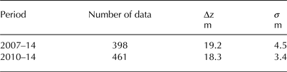
Calibration is necessary for DEMs derived using satellite photogrammetry (Bolch and others, Reference Bolch, Pieczonka and Benn2011; Nuimura and others, Reference Nuimura, Fujita, Yamaguchi and Sharma2012). We used GPS data (GPS-DEM) to calibrate the DEMs generated from the ALOS PRISM images. The 2007 and 2010 DEMs showed positive biases of 19.2 and 18.3 m for 2010 when compared against the GPS-DEM (Figs 2a, b; Table 2). The vertical coordinates of the DEMs were then corrected for these biases. We attribute this vertical offset to uncertainties in the parameters in the RPC files. The standard deviations (σ) of the DEMs relative to GPS-DEM were σ 2007 = 4.5 m in 2007 and σ 2010 = 3.4 m in 2010 (Table 2). Fukuda and others (Reference Fukuda, Sugiyama, Sawagaki and Nakamura2014) applied the same DEM generation technique to ALOS PRISM images of an Antarctic tidewater glacier and obtained a mean standard deviation of 3.2 m for an ice-free terrain. Thus, our DEMs are of the same quality as those reported in the aforementioned study.
Elevation differences in the ice-free area (a) between 2007 DEM and GPS-DEM and (b) between 2010 DEM and GPS-DEM. The comparisons of the DEMs were made along the GPS survey route off the glacier (Fig. 1d).

The mean elevation difference (Δz) and standard deviation (σ) between the 2007 and 2010 DEMs and the 2014 GPS-DEM on the ice-free terrain on the eastern bank of Bowdoin Glacier
3.3. Surface elevation change and ice volume loss
Elevation change over the glacier surface was computed by subtracting the calibrated DEMs from 2007 and 2010. The glacier outline was manually digitized on the orthorectified ALOS PRISM image. To compute the changes from 2010 to 2013, we interpolated the 2010 DEM grid data into the 2013 GPS survey sites using a cubic interpolation algorithm, allowing us to obtain elevation changes at the GPS survey sites. The uncertainty in the computed surface elevation change from 2007 to 2010 (σ e) was estimated using the quadratic sum of σ 2007 and σ 2010 (Bolch and others, Reference Bolch, Pieczonka and Benn2011):
 $$\sigma _{\rm e} = \sqrt {\sigma _{2007}^2 + \sigma _{2010}^2}. $$
This estimation gives 5.6 m, but the actual error is expected to be smaller because image contrast on ice surfaces is higher than on land, and thus the quality of the elevation data was higher on the glacier than on the ice-free area.
The error is even further reduced when a large number of samples are averaged over an area. The standard error of the mean (σ se) is better suited as an estimate of uncertainty in the mean surface elevation change over a glacier (Berthier and others, Reference Berthier2007; Bolch and others, Reference Bolch, Pieczonka and Benn2011).
 $$\sigma _{{\rm se}} = \displaystyle{{\sigma _{\rm e}} \over {\sqrt n}} $$
Sample size n is the number of TIN nodes over a glacier. According to this calculation, the standard error of the mean over the region studied was ~0.1 m with n = 3276 for the elevation change from 2007 to 2010. The accuracy of the kinematic GPS survey in 2013 (<0.2 m) was smaller than the photogrammetric analysis, and thus uncertainties in the elevation change from 2010 to 2013 can be assumed to be similar or less than those for 2007–10. Ice volume loss due to frontal retreat of Bowdoin Glacier was computed from the calving front positions mapped on the orthorectified 2007 and 2010 ALOS PRISM images and ice thickness (230 m) measured by ice radar survey (Sugiyama and others, Reference Sugiyama, Sakakibara, Tsutaki, Maruyama and Sawagaki2015).
3.4. Ice speed measurement by satellite image analysis
We measured an ice surface velocity field of Bowdoin and Tugto Glaciers by applying the image matching method to Landsat 7 ETM+ and Landsat 8 OLI images (Sakakibara and Sugiyama, Reference Sakakibara and Sugiyama2014). Displacements of glacier surface features were determined by the orientation correlation method in the frequency domain between temporally separated satellite image pairs (Heid and Kääb, Reference Heid and Kääb2012). We used 615 pairs from 107 scenes of Landsat 7 and 8 images acquired between 2 July 2006 and 1 October 2014 with temporal separations of 23–498 d. We eliminated displacement vectors that deviated >30° or >150 m a−1 from a median vector within the neighbouring 5 × 5 or 3 × 3 pixels (Heid and Kääb, Reference Heid and Kääb2012). After this filtering, displacement vectors computed from all the image pairs were weighted for temporal separations and averaged over a year to obtain annual mean ice velocity fields for 2007 to 2013. Measurement errors caused by the image matching method consist of (1) ambiguities in the cross-correlation peak, (2) co-registration errors and (3) false correlations (Howat and others, Reference Howat, Box, Ahn, Herrington and McFadden2010). Errors caused by (1) and (2) were estimated from the RMS horizontal displacement of ice-free terrain, where surface displacement should be zero. Errors due to (3) were minimized by applying the filters described above. The accuracy of the resultant speed is dependent on the quality and temporal separation of the images, and the number of image pairs available in each period. For example, accuracy in the annual mean ice speed 3.5 km up-glacier from the calving front (B1403 in Fig. 1d) was ± 12 m a−1.
3.5. Surface mass balance
SMB was measured on Tugto Glacier at IF1207 (512 m a.s.l.) and IF1208 (324 m a.s.l.) from 30 July 2012 to 15 July 2013 (Fig. 1c), and on Bowdoin Glacier at B1403 (123 m a.s.l.), B1413 (109 m a.s.l.) and BH1 (71 m a.s.l.) from 19 July 2014 to 16 July 2015 (Fig. 1d). These sites were all located in the ablation area. 2 m long aluminum poles were installed in the ice surface using a mechanical ice drill (Kovacs) equipped with an electric drill driver (Makita HR262DRDX). We measured the height of the poles above the ice surface (e.g. Fischer and others, Reference Fischer2011). To compare it with observed surface elevation change, SMB was computed into metre ice equivalent using the ice density of 917 kg m−3. The accuracy of the SMB measurements was <50 mm (Østrem and Stanley, Reference Østrem and Stanley1969).
4. RESULTS
4.1. Surface elevation change and ice volume loss
DEMs depict details of surface features on Bowdoin Glacier (Fig. 1d). For example, the ice surface near the eastern margin at the lowermost profile T1 is slightly elevated relative to the western half of the glacier. From this point, ice surface is inclined up-glacier. Along the upper profile T3, the surface is sloping from east to west, under the influence of inflow from a tributary merging from the east.
Surface elevation dropped from 2007 to 2010 over the entire area studied at a mean rate of −2.8 ± 0.1 m a−1 (Fig. 3). At Bowdoin Glacier, decrease in surface elevation is most significant within an area 8 km from the terminus (−8 to −2 m a−1) and the mean rate within 10 km from the terminus was −4.1 ± 0.3 m a−1. The greatest change occurred at the central part of the calving front with a mean rate of −6.6 ± 1.0 m a−1. The magnitude of the elevation change decreases up-glacier. The change was particularly small in the eastern tributary and the upper reaches (within 8–10 km from the terminus) of Bowdoin Glacier, where the rate of change was within the range of −4 to 0 m a−1. Relatively large decrease in surface elevation was observed near the terminus of Tugto Glacier. Apart from these regions, the magnitude of thinning over Tugto Glacier (mean rate of 2.8 ± 0.3 m a−1) was generally smaller than that of Bowdoin Glacier.
The rate of surface elevation change over Bowdoin and Tugto Glaciers between 20 August 2007 and 4 September 2010. The glacier margin was determined from the 2010 satellite image. The background is an ALOS PRISM image taken on 4 September 2010.

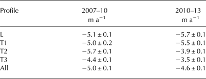
Figures 4a, b show the surface elevation change of Bowdoin Glacier along the GPS profiles L and T1–T3 for the 2007–10 and 2010–13 periods (Table 3). Between 2010 and 2013, the glacier thinned at rates between 0 to 8 m a−1. Relatively large surface elevation change (from −8 to −4 m a−1) occurred along T1 and lower half of L. Figure 4c shows the change in the rate from 2007–10 to 2010–13. The rate of surface elevation lowering slightly increased along L (from 5.1 to 5.7 m a−1) and T1 (from 5.0 to 5.5 m a−1). Deceleration in the rate of surface elevation lowering was clearly observable in the western half of the profile T2. In this region, the thinning rate in 2010–13 was 30% of that seen in 2007–10.
(a) The rate of surface elevation change along the GPS profiles L and T1–T3 over the periods from 2007 to 2010 and (b) 2010–13. (c) Change in the rate from 2007–10 to 2010–13 ((b) − (a)).

The rate of mean elevation change along the profiles L and T1–T3 on Bowdoin Glacier for the periods of 2007–10 and 2010–13
Ice volume change of Bowdoin and Tugto Glaciers over the area studied (294.8 km2) for time period between 2007 and 2010 was −3.58 ± 0.39 km3. Over the same period, Bowdoin Glacier lost an area of 2.34 km2 at the front and associated ice volume loss was 0.54 ± 0.02 km3. As a result, total ice loss in the area we studied was 4.12 ± 0.41 km3.
4.2. Surface mass balance
SMB on Tugto Glacier for 2012/13 was −0.76 m a−1 at IF1207 and −0.89 m a−1 at IF1208 (Fig. 5). SMB on Bowdoin Glacier for 2014/15 was −1.77, −1.90 and −1.96 m a−1 at B1403, B1413 and BH1, respectively. These results cover the SMB over an elevation range from 71 to 512 m a.s.l. Assuming that mass-balance conditions were similar in 2012/13 and 2014/15, the elevation dependence of the SMB is −0.35 m (100 m)−1 (Fig. 5).
Altitudinal distribution of surface mass balance (SMB) for Tugto Glacier in 2012/13 (blue diamonds) and Bowdoin Glacier in 2014/15 (red squares). Red and blue circles are mean rates of surface elevation change (dh/dt) of Bowdoin and Tugto Glaciers for 2007–10 for 20 m bins. The error bars indicate the standard deviations within the bins. Dashed line is the linear regression of SMB data on Tugto and Bowdoin Glaciers.

4.3. Ice speed
Figure 6 shows the annual mean velocity field in 2007. On Bowdoin Glacier, surface speed increases down-glacier from ~40 m a−1 in the upper reaches to a maximum of 428 ± 12 m a−1 near the centre of the calving front. Ice speed is greater in the western half of the glacier, which is influenced by the deep trough located off the glacier centre (Sugiyama and others, Reference Sugiyama, Sakakibara, Tsutaki, Maruyama and Sawagaki2015). The glacier surface is heavily crevassed in this region as a result of shearing due to a speed gradient towards the margin (satellite image in Fig. 1d). Tugto Glacier flows significantly slower than Bowdoin Glacier, typically at 20–100 m a−1. Ice speed progressively decreases down-glacier within 7 km of the terminus and the ice diverges as the glacier width increases down-glacier.

(a) Surface ice speed and (b) longitudinal strain rate averaged over 2007–13 along the flowlines on Bowdoin and Tugto Glaciers (Fig. 6). The strain rate was filtered with a local regression smoothing routine with a bandwidth of 700 m. (c) Bed and surface elevations are as in 2010. (d) Observed elevation change and estimated dynamically-induced elevation change along the flowline of Bowdoin Glacier and (e) Tugto Glacier.

(a) Surface elevation along the flowline on Bowdoin Glacier (Fig. 6) in 2007 (black), 2010 (red), 2013 (blue) and bedrock topography (dashed line). (b) The driving stress along the flowline in 2007 (black), 2010 (red) and 2013 (blue). Solid curves in (a) were obtained by filtering the data with a local regression smoothing routine with a bandwidth of 700 m. Dots in (a) are locations of the GPS and ice radar survey.

5. DISCUSSION
5.1. Thinning of Bowdoin Glacier
Our results revealed rapid thinning of Bowdoin Glacier over the study period. The mean rate of surface elevation change obtained in this study (−4.1 ± 0.3 m a−1 for 2007–10) is similar to values reported for a portion of Bowdoin Glacier based on laser altimetry measurements (−5.0 ± 0.1 m a−1 for 2009–12; Khan and others, Reference Khan2014). Bowdoin Glacier is thinning more rapidly than neighbouring marine-terminating outlet glaciers in the Qaanaaq region. For example, on Heilprin, Melville, Hubbard, Verhoeff and Morris Jesup Glaciers, which are located within 70 km from Bowdoin Glacier (Fig. 1b), surface elevation changed at rates <−3 m a−1 for 2009–12 (Khan and others, Reference Khan2014). The thinning rate at Bowdoin Glacier is slightly smaller than that observed at Tracy Glacier (6 m a−1 for 2009/10) (Porter and others, Reference Porter2014), the most rapidly changing glacier among those flowing into Inglefield Bredning, the largest fjord in the Qaanaaq region (Fig. 1b). The thinning of Bowdoin Glacier is comparable with those reported for outlet glaciers along Melville Bay, located at 72.5°–76.5°N and 200–500 km south from our study site (>4 m a−1 for 2005–10) (Kjær and others, Reference Kjær2012; Kjeldsen and others, Reference Kjeldsen2013). Walsh and others (Reference Walsh, Howat, Ahn and Enderlin2012) studied elevation change of 28 glaciers in central eastern Greenland. The mean rate 15 km from the glacier termini was −15.6 to −0.3 m a−1 from 2000 to 2010.
5.2. Mechanism for the rapid thinning of Bowdoin Glacier
The thinning rate of Bowdoin Glacier was 1.5 times greater than that of land-terminating Tugto Glacier. Because Bowdoin and Tugto Glaciers are only ~3 km apart and at a similar altitude range (Fig. 1c), we would expect the surface melt induced thinning to be similar. Moreover, the negative SMB observed in this study accounts for only <40% of the surface elevation change on Bowdoin Glacier for 2007–10 (Fig. 5). This implies that the rapid thinning of Bowdoin Glacier is affected by ice dynamics. To quantify the contribution of ice dynamics to the observed thinning, we analyse the ice flow speed of Bowdoin and Tugto Glaciers.
Figure 7a shows the mean flow speed for 2007–13 along the flowline of Bowdoin and Tugto Glaciers (Fig. 6 for the location of the flowlines). The ice speed of Bowdoin Glacier increases towards the glacier front, indicating a stretching ice flow regime in the region. Within ~3500 m of the front of Bowdoin Glacier, crevasses are formed perpendicular to the ice flow direction as observed in satellite images (Fig. 1d). Formation of the transverse crevasses is an indication of a longitudinal stretching ice flow regime, which is typically observed near the front of calving glaciers (Vieli and others, Reference Vieli, Funk and Blatter2000; O'Neel and others, Reference O'Neel, Echelmeyer and Motyka2001; Benn and others, Reference Benn, Warren and Mottram2007a). On the other hand, a decrease in speed as we move toward the terminus of Tugto Glacier indicates a compressive flow regime. To examine the influence of these contrasting flow regimes of marine- and land-terminating glaciers on ice thinning, we calculated longitudinal strain rate along the flowline of Bowdoin and Tugto Glaciers (Fig. 7b). At Bowdoin Glacier, the strain rate increases down-glacier and reaches ~0.043 a−1 ~4000 m from the terminus. Ice thickness change in time (∂H/∂t) caused by imbalance of ice flux along the flowline was calculated by
 $$\displaystyle{{\partial H} \over {\partial t}} = - H\displaystyle{{\partial \bar u} \over {\partial x}} - \bar u\displaystyle{{\partial H} \over {\partial x}}$$
where ū is mean flow velocity over the ice thickness (here we assume surface velocity × 0.9) and x is the coordinate along the flowline (Cuffey and Paterson, Reference Cuffey and Paterson2010). We neglect the change in the glacier width in Eqn (3). Figure 7c shows surface elevation of Bowdoin and Tugto Glaciers in 2010 and bed elevation of Bowdoin Glacier used for the computation of H. The bed elevation was measured in the field by ground based ice radar survey (Sugiyama and others, Reference Sugiyama, Sakakibara, Tsutaki, Maruyama and Sawagaki2015). Since no bed elevation data were available in Tugto Glacier, the bed elevation was assumed to be same as that of Bowdoin Glacier. This crude assumption is based on similarities in width, length and surface slope of the two glaciers (Fig. 1c). To avoid the influence of the small-scale surface roughness on the computation, the ice surface elevation surveyed was filtered with a local regression smoothing routine with a bandwidth of 700 m (approximately equal to twice the ice thickness in the region). For the same reason, we applied linear regression to the bed elevation. For Bowdoin Glacier, the thinning rate caused by ice dynamics is estimated to be 3.0–4.5 m a−1 in the region between T1 and T3 (Fig. 7d). Given that measured SMB was −2.0 m a−1 in this region (Fig. 5), summation of the dynamic thinning and negative SMB agrees with the observed surface lowering within the uncertainty range. The dynamic thinning accounts for on average 60% of the observed surface elevation change between 2007 and 2010. This contribution of the dynamic thinning to the total elevation change of Bowdoin Glacier is comparable with the value (~60%) reported as a mean over the Qaanaaq region for 2006–09 (Khan and others, Reference Khan2015).
In contrast to Bowdoin Glacier, the longitudinal strain rate in Tugto Glacier was small. It ranged from −0.005 to 0.001 a−1 within 6000 m of the terminus (Fig. 7b), which corresponds to an ice thickness change of +0.8 to −0.1 m a−1 (Fig. 7e). The dynamically induced thickening counterbalances negative SMB, resulting in less significant surface elevation lowering compared with Bowdoin Glacier. The measured surface lowering rate (from 2.0 to 3.0 m a−1) is larger than the sum of the dynamic thinning rate and SMB. This is probably due to transverse stretching, which we neglected in Eqn (3). It is also likely that the ice thickness of Tugto Glacier was overestimated in the calculation since we assumed the same bed elevation as that of Bowdoin Glacier.
5.3. Effect of ice thinning on the ice dynamics of Bowdoin Glacier
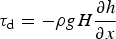
Fast ice flow near the terminus of a marine-terminating outlet glacier can be attributed to basal ice motion (Benn and others, Reference Benn, Warren and Mottram2007a), which is dependent on the driving stress (e.g. Howat and others, Reference Howat, Joughin and Scambos2007; Joughin and others, Reference Joughin2008). Bowdoin Glacier has been thinning over the observation period, which could have caused reduction in the driving stress. This implies a negative feedback between the thinning and ice speed, i.e. glacier thinning causes a decrease in ice discharge from the terminus and reduces ice thinning. On the other hand, the observed thinning rate was greater down-glacier (Fig. 3), which implies a steepening of the glacier and an increase in the driving stress. In this case, thinning near the front causes acceleration and thus drives further dynamic thinning. To examine the influence of ice thinning and surface steepening on the ice dynamics of Bowdoin Glacier, we calculate the driving stress τ d along the flowline within 6 km from the ice front, thus:
 $$\tau _{\rm d} = - \rho gH\displaystyle{{\partial h} \over {\partial x}}$$
where ρ = 917 kg m−3 is the density of ice, g = 9.81 m s−2 is the gravitational acceleration and h is surface elevation. Surface and bed elevation was filtered with a local regression smoothing routine with a bandwidth of 700 m (Fig. 8a). Ice thinning from 2007 to 2013 was 26–47 m (Fig. 8a), which corresponds to 6–15% of the ice thickness in 2007. During the same period, mean surface slope over the analysed 5.3 km-long section increased by 16% from 2.7 × 10⁻² to 3.2 × 10⁻². As a consequence of the thinning and steepening, mean driving stress increased slightly from 79 to 83 kPa (+4%) (Fig. 8b). Although the glacier experienced rapid thinning, the driving stress was unchanged or even increased during 2007–13, suggesting that surface steepening played a dominant role in sustaining a fast flowing condition. The driving stress further increased by ~26% from 2010 to 2013 within x = 3500–6000 m (Fig. 8b). This increase is due to less significant thinning at x = 4000–6000, compared with the lower reaches, which enhanced surface steepening (Fig. 8a).
In addition to the driving stress, the effective pressure (ice-overburden minus basal water pressure) is another control on the basal ice motion. Assuming a constant basal water pressure, the effective pressure decreases as the glacier thins. A decrease in the effective pressure causes glacier acceleration, as seen previously near the front of a calving glacier (Sugiyama and others, Reference Sugiyama2011). Decreases in the effective pressure also enhance shearing in a water-saturated till layer beneath the glacier (Cuffey and Paterson, Reference Cuffey and Paterson2010). Sugiyama and others (Reference Sugiyama, Sakakibara, Tsutaki, Maruyama and Sawagaki2015) reported that the terminus of Bowdoin Glacier is grounded, but very close to flotation, i.e. 86–89% of the entire ice thickness was below sea level in the summer of 2013. It is likely that acceleration and enhanced longitudinal stretching near the terminus resulted in ice thinning and a decrease in effective pressure, which in turn lead to further glacier acceleration (Meier and Post, Reference Meier and Post1987; Vieli and others, Reference Vieli, Funk and Blatter2001; Benn and others, Reference Benn, Hulton and Mottram2007b; Tsutaki and others, Reference Tsutaki, Sugiyama, Nishimura and Funk2013). Therefore, we conclude that a fast flowing condition was maintained by an increase in the driving stress due to surface steepening and a decrease in effective pressure caused by ice thinning.
6. CONCLUSION
To better understand the contribution of ice dynamics to recent thinning of marine-terminating outlet glaciers in northwestern Greenland, we carried out field and satellite-based measurements in Bowdoin Glacier and adjacent land-terminating Tugto Glacier. Surface elevations were measured in 2013 by a GPS survey in the lower 3.3 km of Bowdoin Glacier. The measured elevations were compared with DEMs of 2007 and 2010 generated by photogrammetry of ALOS PRISM imagery.
Bowdoin Glacier has experienced a rapid lowering in its surface elevation from 2007 to 2010 with an average rate of 4.1 ± 0.3 m a−1. The mean rate of elevation change was 1.5 times larger than on Tugto Glacier. The magnitude of elevation change increases down-glacier, reaching −6.6 ± 1.0 m a−1 near the calving front. The observed negative SMB corresponds to <40% of the elevation change of Bowdoin Glacier, therefore rapid thinning is not entirely due to surface melting.
Ice flow fields indicated a longitudinal stretching flow regime near the terminus of Bowdoin Glacier. The dynamic ice thinning estimated from the ice speed field and thickness accounts for 60% of surface elevation change from 2007 to 2010. Thus, more than half the elevation change was caused by ice dynamics. We examined the influence of surface steepening and thinning on ice dynamics near the terminus. Driving stress increased by 4% over the period from 2007 to 2013, suggesting the effect of surface steepening was greater than that of thinning, resulting in consistently fast ice flow from 2007 to 2013. Most likely, the effective pressure at the glacier bed decreased because of the ice thinning, and this also enhanced basal motion, particularly near the terminus. These observations indicate that rapid thinning observed in marine-terminating Bowdoin Glacier was largely affected by the ice dynamics, i.e. enhanced longitudinal stretching ice flow caused by acceleration near the glacier terminus.
ACKNOWLEDGEMENTS
We thank the members of the 2013–15 field campaigns in Qaanaaq. Special thanks are owed to S. Daorana and T. Oshima for providing logistic support in Qaanaaq. The manuscript was handled by Scientific Editor, Martyn Tranter, and carefully commented by two anonymous reviewers. We appreciate Chief Editor, Jo Jacka, who has gently edited the manuscript toward publication. This research was funded by MEXT (Japanese Ministry of Education, Culture, Sports, Science and Technology) through the Green Network of Excellence (GRENE) Arctic Climate Change Research Project and the Arctic Challenge for Sustainability (ArCS) Project. We thank H. Enomoto for his contribution as the leader of the GRENE project.


 Open access

