


Impact statement
Rangeland ecosystems deliver vital ecosystem services (ESs), including instrumental benefits such as food and fiber from livestock. Additionally, rangelands may contribute to human well-being through intrinsic or non-monetary ES values. Rangelands also support a distinct potential biodiversity that plays a crucial role in regulating climate and hydrological cycles, which underpin numerous cultural ESs. The concept of ESs has been fundamental in various high-level policy frameworks, such as the Convention on Biological Diversity, the Intergovernmental Platform on Biodiversity and Ecosystem Services, the World Bank’s Global Partnership for Wealth Accounting, the Valuation of Ecosystem Services, and the EU Biodiversity Strategy. However, the application of the ES framework at the regional scale within Latin America has been limited, with the notable exception of the Natural Capital Trust in Costa Rica (Hernández-Blanco et al., Reference Hernández-Blanco, Costanza and Moritsch2025). In this context, mapping potential biodiversity values and ES at the landscape level in Southern Patagonia represents an important step toward a better understanding of potential trade-offs and synergies between management and conservation strategies. The mapping and analyses presented here fill some of these gaps and aim to enhance current land use planning efforts.
Introduction
The concept of ecosystem services (ESs) seeks to elucidate the diverse benefits that humans obtain from nature. This includes provisioning ES, which are related to tangible products directly consumed by humans that possess identifiable market values, such as wool, food and clean water. Additionally, ES encompasses more intangible benefits, including aesthetic appreciation, recreation, ecotourism, artistic inspiration and a sense of place (MEA, 2005; Martínez Pastur et al., Reference Martínez Pastur, Peri, Lencinas, García Llorente and Martín López2016a). Biodiversity is central to the provision of ES due to the ecological functions and processes that the different species sustain (Daily, Reference Daily1997), however, the links between biodiversity and ES will also be determined by the interplay between demand and supply (Yahdjian et al., Reference Yahdjian, Sala and Havstad2015). Thus, while previous research was concentrated on how much ES are produced (supply), sustainable management requires addressing the gap between this supply and what society needs (demand). The provision of ES from rangeland ecosystems in the Global South has received comparatively limited research attention (Eldridge et al., Reference Eldridge, Wang, Liu, Ding, Li, Wu and Li2024). Moreover, the interconnections between ES and biodiversity within rangeland ecosystems have rarely been explored (Duarte-Guardia et al., Reference Duarte-Guardia, Peri, Martinez-Pastur, Lasagno, Lencinas, Thomas and Ladd2024).
Vegetation types in Southern Patagonia (Santa Cruz province, Argentina) have been classified and mapped in detail (Peri et al., Reference Peri, Gaitán, Díaz, Almonacid, Morales, Ferrer, Lasagno, Rodríguez-Souilla and Martínez Pastur2024). Steppe grasslands cover the largest extension (58% of the province), with shrubland, dwarf shrubland, Mata Negra Matorral thickets and deciduous Nothofagus forests covering lesser extensions (Peri et al., Reference Peri, Martínez Pastur and Nahuelhual2021a, Reference Peri, Gaitán, Díaz, Almonacid, Morales, Ferrer, Lasagno, Rodríguez-Souilla and Martínez Pastur2024). The human footprint (e.g. roads, infrastructure, livestock grazing, desertification) is variable but has a profound effect on local biodiversity (Rosas et al., Reference Rosas, Peri, Martínez Pastur, Peri, Martínez Pastur and Nahuelhual2021a, Reference Rosas, Peri, Lencina, Lasagno and Martínez Pastur2021b). Extensive sheep grazing is the main land use. Livestock production is heavily dependent on the environment and management (Trier Bjerring et al., Reference Trier Bjerring, Peri, Christiansen, Vargas-Bello-Pérez and Hansen2025). Heavy and unsustainable stocking rates threaten the future of livestock productivity and the long-term viability of the local economy. Broadening the appreciation of the values that rangeland generates to include also potential biodiversity, regulating, supporting and cultural ES could result in more rational management proposals of the natural capital in Southern Patagonia (Peri et al., Reference Peri, Lencinas, Martinez Pastur, Wardell-Johnson, Lasagno, Morales Prieto and Traba Díaz2013; Oñatibia, Reference Oñatibia, Peri, Nahuelhual and Martínez Pastur2021). In this context, the objective was to characterize the generation of ES (cultural, supporting, regulating and provisioning) and potential biodiversity values of different vegetation types in rangeland ecosystems of Santa Cruz province, Argentina and discuss potential synergies and trade-offs among them. We hypothesized that the provision of the different ES is not independent, where interaction occurred among them according to the species assemblage (vegetation types), biophysical characteristics of the ecosystems and human pressures on natural ecosystems due to economic activities generating synergies and trade-offs between ES and biodiversity.
Methods
Study area
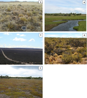
The present work is focused on the grasslands and shrublands ecosystems of the Patagonian steppe in Santa Cruz province (243,943 km2) between latitudes 46°00′ and 52°30’ S (Southern Patagonia, Argentina) (Figure 1). We used the vegetation types proposed by Peri et al. (Reference Peri, Gaitán, Díaz, Almonacid, Morales, Ferrer, Lasagno, Rodríguez-Souilla and Martínez Pastur2024), which include: (i) Steppe grasslands characterized by the presence of tussock grasses (Festuca spp., Pappostipa spp.), short grasses (Poa spp.), graminoids (Carex sp.) and shrubs. These species are the main feed resource for sheep farming (Peri et al., Reference Peri, Rosas, Rivera and Martínez Pastur2021b). The steppe grassland type (Figure 2A) is subdivided into two subcategories: (a) Grass steppe dominated by grasses and sedges (Bromus sp., Carex sp., Festuca spp., Hordeum sp., Pappostipa sp., Poa sp., Rytidosperma sp. and Trisetum sp.) with dwarf shrubs and herbs such as Nardophyllum sp., Perezia sp., Azorella sp. and Nassauvia sp. at lower densities; and (b) grass-shrub steppe dominated by the grasses Pappostipa sp., Agrostis sp., Festuca spp., Hordeum sp., and Trisetum sp. and shrubs (Berberis sp., Adesmia sp., Chuquiraga sp., Azorella prolifera , Mulguraea sp., Schinus sp. and Senecio sp.) with shrubs present at higher densities. (ii) The wetland vegetation type (Figure 2B) dominated by Cyperaceae, Juncaceae and Gramineae species, in areas where water naturally accumulates. Wetlands are the most important vegetation type for livestock production, mainly located on floodplains, glacial plains and on hydro-eolian basins. (iii) Shrublands are dominated by woody plants (>40%) generally less than 3 m in height. Here, we recognize three distinct types: (a) The Mata Negra Matorral thicket (Figure 2C), dominated by the evergreen shrub Mulguraea tridens , which is sclerophyllous and grows in association with xeric steppe vegetation, creating spatial heterogeneity in the landscape because of vegetation patches. (b) The mixed shrublands (Figure 2D) are dominated mainly by tall shrubs, such as Colliguaja integerrima, Chuquiraga, Anartrophyllum rigidum, Lycium sp. and Azorella prolifera . The understory includes grasses such as Bromus sp., Hordeum sp., Pappostipa sp. and Poa sp. (c) Dwarf-shrublands (Figure 2E) are dominated by Empetrum rubrum , which mainly occurs on sites with acidic, coarse-textured and poor nutrient soils. Dwarf shrublands are often heavily disturbed due to overgrazing and fire.
Characterization of the study area: Location of Santa Cruz province (red) and main vegetation types. White areas are bare soil, mountains, forests, water bodies, icefields and snow cover (Peri et al., Reference Peri, Gaitán, Díaz, Almonacid, Morales, Ferrer, Lasagno, Rodríguez-Souilla and Martínez Pastur2024).
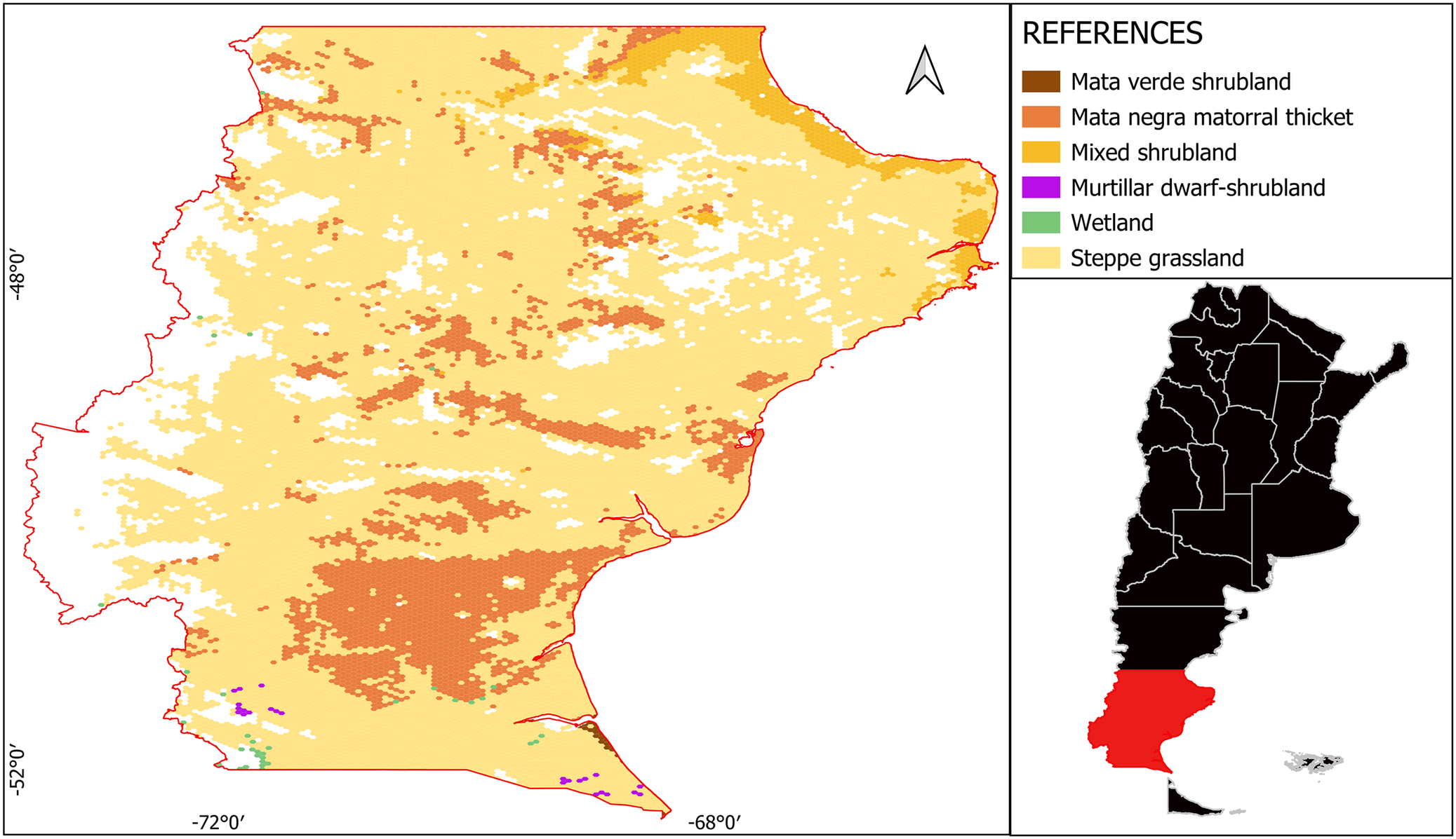
Figure 1. Long description
At the bottom right, an inset map of Argentina highlights Santa Cruz province in red. The main map displays Santa Cruz with vegetation types coded by color: steppe grassland in pale yellow dominates most of the province, especially the north, center, and east. Mixed shrubland in orange is concentrated in the south-central region. Mata verde shrubland in brown appears as scattered patches, mainly in the south. Mata negra matorral thicket in dark brown is found in smaller, denser clusters, especially in the southern and central areas. Murtillar dwarf-shrubland in purple and wetlands in green are limited to small, isolated patches, mostly in the southwest and southeast. White areas represent bare soil, mountains, forests, water bodies, icefields, and snow cover. The legend at the top right lists all vegetation types with corresponding colors.
The main vegetation types in Santa Cruz (Argentina): (A) steppe grassland, (B) wetlands, (C) Mata Negra Matorral thicket, (D) mixed shrubland, and (E) murtillar dwarf-shrubland.
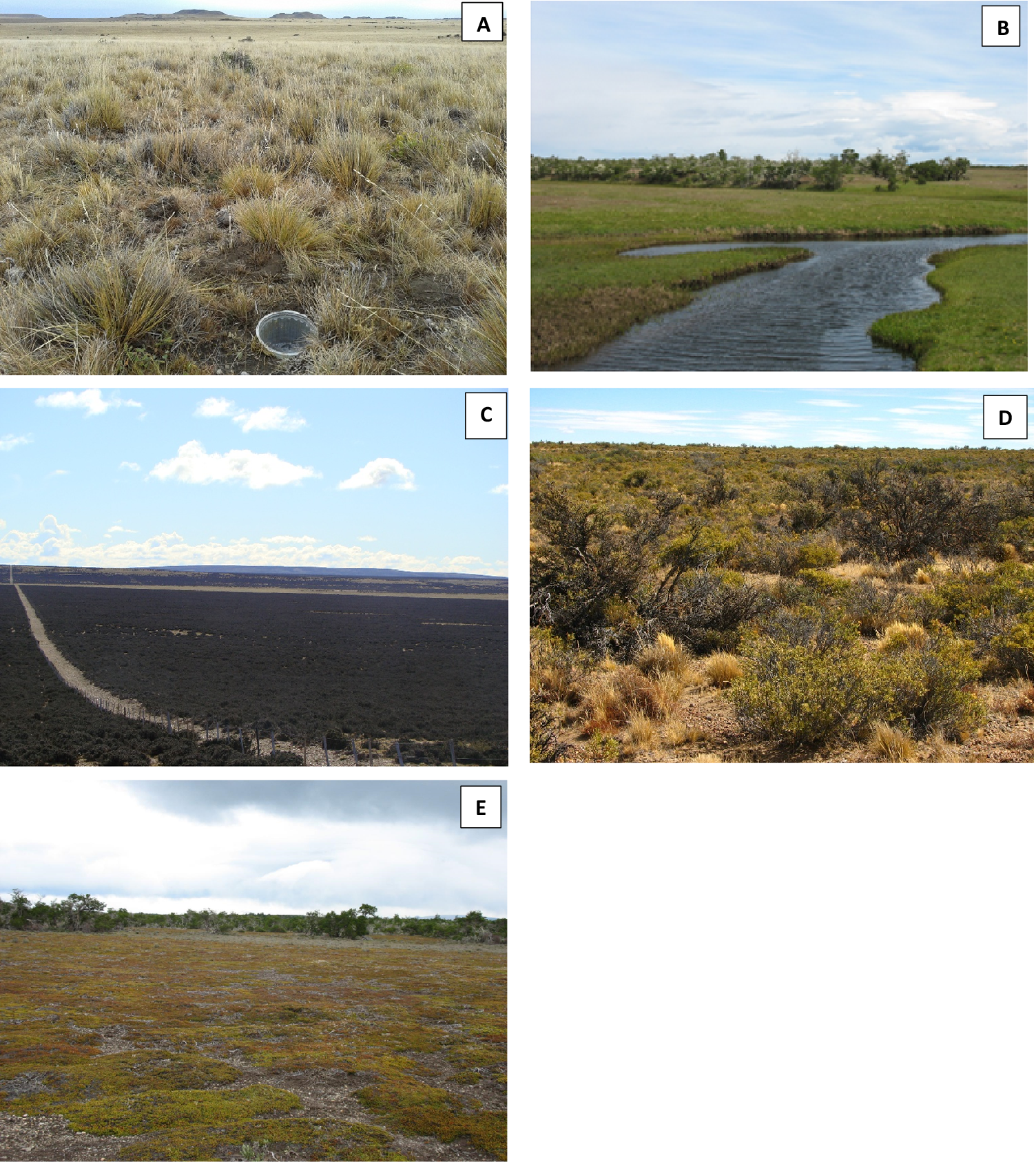
Figure 2. Long description
Panel A at the top left shows steppe grassland with sparse, yellowish tussocks and open soil patches. Panel B at the top right depicts a wetland with a winding water channel bordered by green grass and distant trees under a blue sky. Panel C at the bottom left presents Mata Negra Matorral thicket, characterized by a dark, low shrub cover and a straight fence line dividing the landscape horizontally. Panel D at the bottom right illustrates mixed shrubland with dense, interspersed shrubs and tufts of grass. Panel E at the bottom center displays murtillar dwarf-shrubland, featuring a low, continuous mat of small shrubs and mosses with a flat horizon and overcast sky.
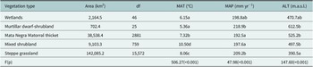
Topographic variables were defined using GIS and the Shuttle Radar Topography Mission data (Farr et al., Reference Farr, Rosen, Caro, Crippen, Duren, Hensley, Kobrick, Paller, Rodriguez, Roth, Seal, Shaffer, Shimada, Umland, Werner, Oskin, Burbank and Alsdorf2007), which produced the highest-resolution digital elevation model. Climatic variables, including temperature, precipitation and annual, monthly and seasonal climate indices were defined using the methods described in Hijmans et al. (Reference Hijmans, Cameron, Parra, Jones and Jarvis2005). The regional climate is arid, cold and windy. Rainfall ranges from 192 to 219 mm yr−1 (Table 1). Mean annual temperature ranges from 5.4 to 10.5 °C (Peri et al., Reference Peri, Lencinas, Bousson, Lasagno, Soler, Bahamonde and Martínez Pastur2016) (Table 1). The wind is predominantly from the south-southwest. Severe and frequent windstorms occur in spring and summer with wind speeds over 100 km h−1. Altitude ranges from sea level to more than 1000 m.a.s.l. (Lencinas et al., Reference Lencinas, Soler, Cellini, Bahamonde, Pérez Flores, Monelos, Martínez Pastur and Peri2021), with average values ranging from 390 to 612 m.a.s.l. depending on the vegetation type (Table 1). Steppe grasslands cover the largest extension in the province (representing 58.1% of the total area of the province or 142,085 km2), followed by Mata Negra Matorral thickets (15.7%, 38,355 km2) (Table 1).
Area of the studied vegetation types, and ANOVAs results for mean annual temperature (MAT), mean annual precipitation (MAP) and altitude (ALT) comparing vegetation types in Santa Cruz province (Argentina)
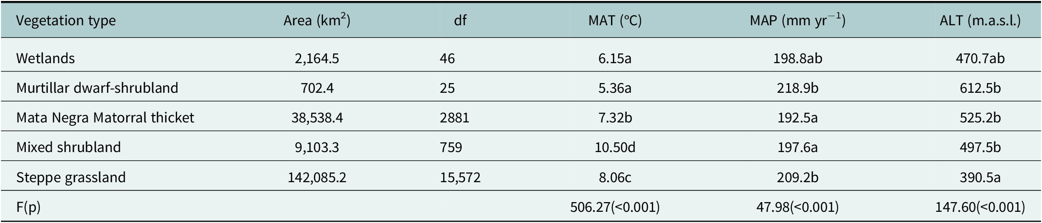
Table 1. Long description
From top to bottom, columns are vegetation type, area in square kilometers, degrees of freedom, mean annual temperature in degrees Celsius, mean annual precipitation in millimeters per year, and altitude in meters above sea level. Wetlands: area 2,164.5, df 46, MAT 6.15 a, MAP 198.8 a b, ALT 470.7 a b. Murtillar dwarf-shrubland: area 702.4, df 25, MAT 5.36 a, MAP 218.9 b, ALT 612.5 b. Mata Negra Matorral thicket: area 38,538.4, df 2,881, MAT 7.32 b, MAP 192.5 a, ALT 525.2 b. Mixed shrubland: area 9,103.3, df 759, MAT 10.50 d, MAP 197.6 a, ALT 497.5 b. Steppe grassland: area 142,085.2, df 15,572, MAT 8.06 c, MAP 209.2 b, ALT 390.5 a. The bottom row shows F and p values for each variable: MAT F 506.27 (less than 0.001), MAP F 47.98 (less than 0.001), ALT F 147.60 (less than 0.001). Different letters in columns indicate significant differences among vegetation types by Tukey's test at p less than 0.05.
F: Fisher’s test; (p): probability; df: degrees of freedom. Different letters in columns show differences among vegetation types according to Tukey’s test at p < 0.05.
Provision of different ecosystem services at the landscape level
We selected eight proxies to quantify the level of ES provision from the different vegetation types: (i) Cultural ES including aesthetic, existence, local identity and recreational values; (ii) Regulating services which used net primary productivity and soil carbon as proxies and supporting services which were measured by characterizing habitat quality (maximum potential habitat suitability for the studied species); and (iii) Provisioning services which were characterized through livestock capacity and oil production.
Four maps were created for the cultural ES, three related to human interactions (e.g. physical or intellectual) with biotic systems, ecosystems and landscapes and another map that relates spiritual values to biotic systems, ecosystems and landscapes. For these maps, we used the methods and data of Martínez Pastur et al. (Reference Martínez Pastur, Peri, Lencinas, García Llorente and Martín López2016a). In short, this methodology used geo-referenced digital photos from a web platform that the public used to upload photos taken in the region. The social and biophysical importance of the cultural ESs in the landscape were evaluated through the quantification of the number of digital images that either local people and/or external visitors to the region uploaded to the Panoramio web platform. Then, we applied the Kernel density tool in a GIS, which allowed us to calculate the density of photos around each cell of a raster. Four proxies were considered: (i) aesthetic values were related to the interaction of people with the environment in relation to natural beauty, based on human perceptions and judgments, (ii) existence values were related to the degree of satisfaction that people get from knowing that a natural resource, like a species or an ecosystem, exists, (iii) local identity values were linked to images that depicted local culture and heritage, and (iv) recreation values were linked to images that captured the recreation value of the natural capital was captured in the image. To assess which social and biophysical variables best explained the spatial distribution of each cultural service (Martínez Pastur et al., Reference Martínez Pastur, Peri, Lencinas, García Llorente and Martín López2016a) each map was rescaled from 0 to 100 using a linear scale by a function tool in ArcMap 10.0 software (ESRI, 2011). The significance of the explanatory variables in the explanation of the associations between cultural ES was tested with a Monte Carlo permutation test with 500 permutations per analysis. The inertia of the factors, which represents the explained variance, was used to identify the most important social and biophysical factors determining the associations between cultural ESs and landscape attributes (Martínez Pastur et al., Reference Martínez Pastur, Peri, Lencinas, García Llorente and Martín López2016a).
Regulating services were estimated using net primary productivity (NPP) as a proxy (g.m−2 yr−1), after Zhao and Running (Reference Zhao and Running2010). The NPP data with a resolution of 30 arc seconds were acquired from the MOD17A3 data released by NASA’s Earth Observation System Data and Information System. In these ecosystems, NPP varied from 30.9 to 714.2 g C/m2/year (Peri et al., Reference Peri, Rosas, Rivera and Martínez Pastur2022). Using the GIS platform, a map with a resolution of 90 × 90 m was constructed to project the regulating services in the landscape. The human footprint index (HFI) was used as a proxy for the supporting services after Rosas et al. (Reference Rosas, Peri, Pidgeon, Martinuzzi, Politi, Pedrana, Díaz Delgado and Martínez Pastur2021c). In a GIS project, supporting services were calculated as the inverse of the Human Footprint Index (1-HFI) values to produce a natural habitat proxy map with a resolution of 90 m × 90 m. SOC was modeled for the first 30 cm of the soil profile by Peri et al. (Reference Peri, Rosas, Ladd, Toledo, Lasagno and Martínez Pastur2018) and mapped in a grid of 90 m× 90 m. In this work, for modelling, Peri et al. (Reference Peri, Rosas, Ladd, Toledo, Lasagno and Martínez Pastur2018) used a stepwise multiple regression to identify which variables among these uncorrelated variables helped to explain SOC variation at the landscape level. Briefly, the model was evaluated through the standard error of estimation (the r2-adj), defined as the average of the difference between predicted and observed values, and the mean absolute error, defined as the average of the difference between predicted and observed absolute values. From the SOC model, a SOC map was obtained for the entire Santa Cruz province, where the variables derived from the multiple linear regression models were integrated into a GIS using ArcMap 10.0 software.
The provisioning services were estimated using a sheep probability map of stocking density estimated from a model of probability of contact with sheep per ranch (0–1 probability km−2) following Pedrana et al. (Reference Pedrana, Bustamante, Rodríguez and Travaini2011). Values close to 0 indicate a low probability of occurrence and values close to 1 high probability. In the GIS project, we applied the focal statistics tool to create a new raster by considering the values within a 10 km. We then applied a mask for forests and protected areas. Oil production was also included as a component of the “provisioning services” estimation, as it is an important economic activity in the region. Oil production was estimated based on oil well density (wells km−2) (Rosas et al., Reference Rosas, Peri, Martínez Pastur, Peri, Martínez Pastur and Nahuelhual2021a). In a GIS project, we calculated the oil well density using a database of 21,426 registered and georeferenced oil wells. The oil well density map presented values from 0 (minimum density) to 8.44 wells km−2 (maximum density), with a mean value of 0.09 wells km−2. Maps were rescaled from the 0–100 linear scale using the same tool described above.
The different ES were then combined to obtain maps for three ES types (cultural, regulating/supporting and provisioning ES). All the rasterized maps were created using ArcMap 10.0 software (ESRI, 2011), and the resulting average values were rasterized again to obtain final values for each ES type from zero (lower provision of the service) to 100 (maximum provision of the service). This maximum provision value of 100 is rarely reached in the field.
Potential biodiversity mapping
Potential biodiversity values for the region are based on the map and analysis of Rosas et al. (Reference Rosas, Peri, Lencina, Lizarraga and Martínez Pastur2022a) for Santa Cruz. Potential biodiversity refers to an area’s capacity to support a diverse range of plant and animal species, often indicating the maximum theoretical biodiversity an ecosystem can maintain based on its environmental conditions (such as climate, energy, and resources). This map uses a large biodiversity database from the PEBANPA Network (Peri et al., Reference Peri, Lencinas, Bousson, Lasagno, Soler, Bahamonde and Martínez Pastur2016). In total, we used 118 maps (90 × 90 m) of potential habitat suitability for five taxonomic groups: one mammal (an endemic deer), 47 species of birds, 7 lizards, 10 darkling beetles and 53 plant species (Rosas et al., Reference Rosas, Peri, Lencina, Lizarraga and Martínez Pastur2022a). Environmental Niche Factor Analysis (Hirzel et al., Reference Hirzel, Hausser, Chessel and Perrin2002) was used to map habitat suitability for each species based on potential physical environmental variables (climate, topography and other variables related to landscape attributes), which were rasterized at 90 m × 90 m resolution using the nearest resampling technique in ArcMap 10.0 (ESRI, 2011) using Biomapper 4.0 software (Hirzel and Le Lay, Reference Hirzel and Le Lay2008). We then used the Cell Statistics tool to combine the 119 potential habitat suitability maps to obtain average values for each pixel, integrating the information for the different taxonomic groups. We first produced five taxonomic group maps: four were maps of potential biodiversity for birds, lizards, darkling-beetles and plants) and the 5th map describes potential habitat suitability for the endemic deer. Then, we created taxonomic group indices (G Indices) to weight each taxonomic group map, considering ecological and endemism values (Rosas et al., Reference Rosas, Peri, Lencina, Lizarraga and Martínez Pastur2022a). These maps were rasterized to present scores that varied between 0 and 100 (average values of potential habitat suitability for all the studied taxa). A map of potential biodiversity (all taxa) was produced by summing values for each pixel of the five weighted maps of the taxonomic group indices in a single GIS project.
Data analysis
We analyzed the different maps of ES and biodiversity using the hexagonal binning and univariate ANOVAs. Hexagonal binning is a method of aggregating individual data (pixel values) into polygonal regions (Battersby et al., Reference Battersby, Strebe and Finn2017). This spatial methodology can simply and effectively represent complex data sets, improving the ability to analyze and visualize spatial patterns (Briney, Reference Briney2014). For this, we calculated for each hexagonal area (250 thousand ha for the provincial scale) the average values of cover for the different vegetation types, environmental variables, ESs and the potential biodiversity (0–100). Explanatory variables, model outputs and statistical fit analyses are described in detail by Rosas et al. (Reference Rosas, Peri, Martínez Pastur, Peri, Martínez Pastur and Nahuelhual2021a, Reference Rosas, Peri, Lencina, Lasagno and Martínez Pastur2021b, Reference Rosas, Peri, Pidgeon, Martinuzzi, Politi, Pedrana, Díaz Delgado and Martínez Pastur2021c, Reference Rosas, Peri, Lencina, Lizarraga and Martínez Pastur2022a, Reference Rosas, Martínez Pastur and Peri2022b).
Results and discussion
Cultural ecosystem services
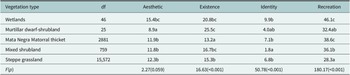
The importance of the various vegetation types that populate the steppe for the supply of cultural ES is low, but it varies in subtle and important ways (Table 2). For example, mean aesthetic and recreational values were highest in wetlands. This result is consistent with previous studies, as there is a positive effect of water presence on aesthetic values and recreation (Abildtrup et al., Reference Abildtrup, Garcia, Olsen and Stenger2013; García-Llorente et al., Reference García-Llorente, Martín-López, Iniesta-Arandia, López-Santiago, Aguilera and Montes2012). Also, the positive effect of vegetation on social preferences toward wetlands can be interpreted as an expression of phytophilia, which is the phenomenon of people generally preferring green views over arid or semiarid landscapes (López-Santiago et al., Reference López-Santiago, Oteros Rozas, Martín-López, Plieninger, González and González2014). Existence values were highest in the dwarf-shrublands, and local identity values were highest for Mata Negra Matorral thicket and steppe grasslands (Table 2). Similarly, Martínez Pastur et al. (Reference Martínez Pastur, Peri, Lencinas, García Llorente and Martín López2016a) reported that the grassland ecosystem positively influenced local identity in Tierra del Fuego because of the historical and cultural importance of ranching.
ANOVAs for aesthetic, existence, local identity and recreation ES comparing vegetation types in Santa Cruz province (Argentina)
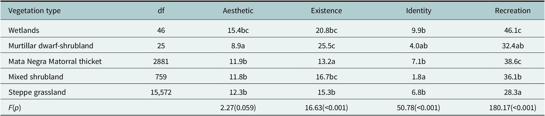
Table 2. Long description
The table lists five vegetation types vertically: Wetlands, Murtillar dwarf-shrubland, Mata Negra Matorral thicket, Mixed shrubland, and Steppe grassland. Columns from left to right are Vegetation type, degrees of freedom (df), Aesthetic, Existence, Identity, and Recreation. For Wetlands: df 46, Aesthetic 15.4 b c, Existence 20.8 b c, Identity 9.9 b, Recreation 46.1 c. For Murtillar dwarf-shrubland: df 25, Aesthetic 8.9 a, Existence 25.5 c, Identity 4.0 a b, Recreation 32.4 a b. For Mata Negra Matorral thicket: df 2881, Aesthetic 11.9 b, Existence 13.2 a, Identity 7.1 b, Recreation 38.6 c. For Mixed shrubland: df 759, Aesthetic 11.8 b, Existence 16.7 b c, Identity 1.8 a, Recreation 36.1 b. For Steppe grassland: df 15,572, Aesthetic 12.3 b, Existence 15.3 b, Identity 6.8 b, Recreation 28.3 a. The bottom row shows F and p values for each ES: Aesthetic F 2.27 (p 0.059), Existence F 16.63 (p less than 0.001), Identity F 50.78 (p less than 0.001), Recreation F 180.17 (p less than 0.001). Numbers range from 0 to 100. Different letters indicate significant differences among vegetation types by Tukey’s test at p less than 0.05.
Note: Numbers varied between 0 (minimum provision) and 100 (maximum provision).
F = Fisher’s test, (p) = probability, df = degrees of freedom. Different letters in columns show differences among vegetation types according to Tukey’s test at p < 0.05.
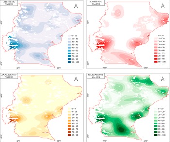
Cultural ESs (Figure 3) were primarily influenced by accessibility and landscape characteristics (Martínez Pastur et al., Reference Martínez Pastur, Peri, Lencinas, García Llorente and Martín López2016a). High values were associated with features possessing significant aesthetic, recreational or ecotourism appeal, such as mountains or lakes. Hotspots were observed in areas where natural marvels are present, including penguin colonies, National Parks and Natural Reserves, whereas cold spots were most prevalent in regions lacking road access. Homogeneous flat landscapes, such as the steppe grasslands, also registered low scores for cultural ES, possibly in part due to limited accessibility and absence of roads. This pattern may be attributed to the limited ability of people to reach these natural ecosystems, underscoring the importance of both demand and supply factors (Yahdjian et al., Reference Yahdjian, Sala and Havstad2015). Finally, homogeneous flat landscapes, like the steppe, are extensive across the studied region, and these landscapes may harbor a great variety of vegetation types.
Cultural ecosystem services (aesthetic, existence, local identity and recreational values) modeled for grasslands and shrublands in Santa Cruz province (Argentina) based on Martínez Pastur et al. (Reference Martínez Pastur, Peri, Lencinas, García Llorente and Martín López2016a). Numbers varied between 0 (minimum provision) and 100 (maximum provision).

Figure 3. Long description
Starting at the top-left, the Aesthetic Values panel uses a blue gradient from light (0–10) to dark (90–100), with highest values concentrated in the southwest. The top-right Existence Values panel uses a red gradient, with highest values (90–100) in the southwest and moderate peaks in the east. The bottom-left Local Identity Values panel uses an orange gradient, with highest values (82–93) in the southwest and lower values elsewhere. The bottom-right Recreational Values panel uses a green gradient, with the highest values (90–100) in the south-central region. All panels share the same map outline of Santa Cruz province, oriented north-up, with value legends and red boundary lines.
Regulating and supporting ecosystem services
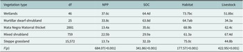
The importance of the various vegetation types in regulating and supporting ES is shown in Table 3. For example, wetlands had the highest SOC, NPP and habitat quality values (Table 3). This is consistent with Ma et al. (Reference Ma, Woolf, Fan, Qiao, Li and Lehmann2023) who also report that SOC supports the capacity of the land to sustain plant productivity. The strong and direct relationship between rainfall and SOC may be related to the NPP and mean soil water content (Peri et al., 2018). The high habitat quality of wetlands is consistent with Rosas et al. (2002a) who reported that plant and bird species had the highest potential biodiversity values, mostly related to humid steppes and shrublands associated with higher NDVI values.
ANOVAs for regulating (NPP: net primary productivity, and SOC: soil carbon stock), supporting (Habitat) and provisioning (Livestock) values of steppe grasslands and shrublands in Santa Cruz province (Argentina)
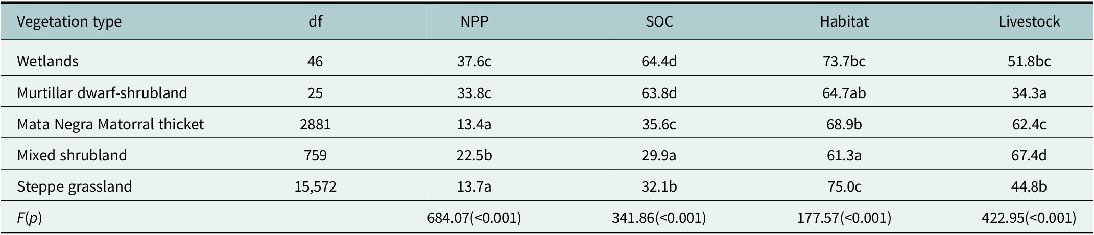
Table 3. Long description
Starting from the top row, the table lists vegetation types: Wetlands, Murtillar dwarf-shrubland, Mata Negra Matorral thicket, Mixed shrubland, and Steppe grassland. For Wetlands, degrees of freedom is 46, N P P is 37.6 c, S O C is 64.4 d, Habitat is 73.7 b c, Livestock is 51.8 b c. Murtillar dwarf-shrubland has 25 degrees of freedom, N P P 33.8 c, S O C 63.8 d, Habitat 64.7 a b, Livestock 34.3 a. Mata Negra Matorral thicket shows 2881 degrees of freedom, N P P 13.4 a, S O C 35.6 c, Habitat 68.9 b, Livestock 62.4 c. Mixed shrubland has 759 degrees of freedom, N P P 22.5 b, S O C 29.9 a, Habitat 61.3 a, Livestock 67.4 d. Steppe grassland has 15,572 degrees of freedom, N P P 13.7 a, S O C 32.1 b, Habitat 75.0 c, Livestock 44.8 b. The final row presents F (p) values: N P P 684.07 (less than 0.001), S O C 341.86 (less than 0.001), Habitat 177.57 (less than 0.001), Livestock 422.95 (less than 0.001). Numbers range from 0 to 100, with different letters indicating significant differences among vegetation types by Tukey's test at p less than 0.05.
Note: Numbers varied between 0 (minimum provision) and 100 (maximum provision).
F = Fisher’s test, (p) = probability, df = degrees of freedom. Different letters in columns show differences among vegetation types according to Tukey’s test at p < 0.05.
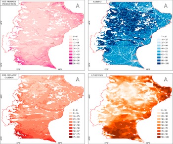
According to Rosas et al. (Reference Rosas, Martínez Pastur and Peri2022b) regulating ES (e.g. NPP) was highest in the south, with a tendency to increase across a gradient of rainfall from east to west (Figure 4). The northwest corner of the province was also a hotspot for regulating services, and here, mixed shrubland was the main vegetation type (Figure 4). Also, according to Rosas et al. (Reference Rosas, Martínez Pastur and Peri2022b), NPP values were greater in valleys and decreased with altitude, with the lowest values recorded in alpine grasslands. The map of SOC showed a continuous decline from the northeast and central areas of Santa Cruz province, dominated by shrublands (Peri et al., 2018), to the south and southwest, where rangelands dominate (Figure 4). There were, however, subtle variations due to the fact that dwarf-shrubland and wetlands, both vegetation types with low vegetation cover, presented higher SOC values, presumably due to more limited decomposition/anoxia (Peri et al., Reference Peri, Gaitán, Díaz, Almonacid, Morales, Ferrer, Lasagno, Rodríguez-Souilla and Martínez Pastur2024). The supporting services of habitat quality decreased as the human footprint increased, mainly due to roads (Rosas et al., Reference Rosas, Peri, Pidgeon, Martinuzzi, Politi, Pedrana, Díaz Delgado and Martínez Pastur2021c). Therefore, the highest values for supporting services are found in the center and west of the province (Figure 4). Complex geomorphology (center) and flooding at the base of the Andes on the western margin of the province may explain the lack of transport infrastructure, low values of ranching activity, and the high levels of supporting services in these locations (Rosas et al., Reference Rosas, Peri, Pidgeon, Martinuzzi, Politi, Pedrana, Díaz Delgado and Martínez Pastur2021c).
Regulating (net primary productivity, soil carbon stock), supporting (habitat) and provisioning (livestock) ecosystem services for grasslands and shrublands in Santa Cruz province (Argentina). Numbers varied between 0 (minimum provision) and 100 (maximum provision).
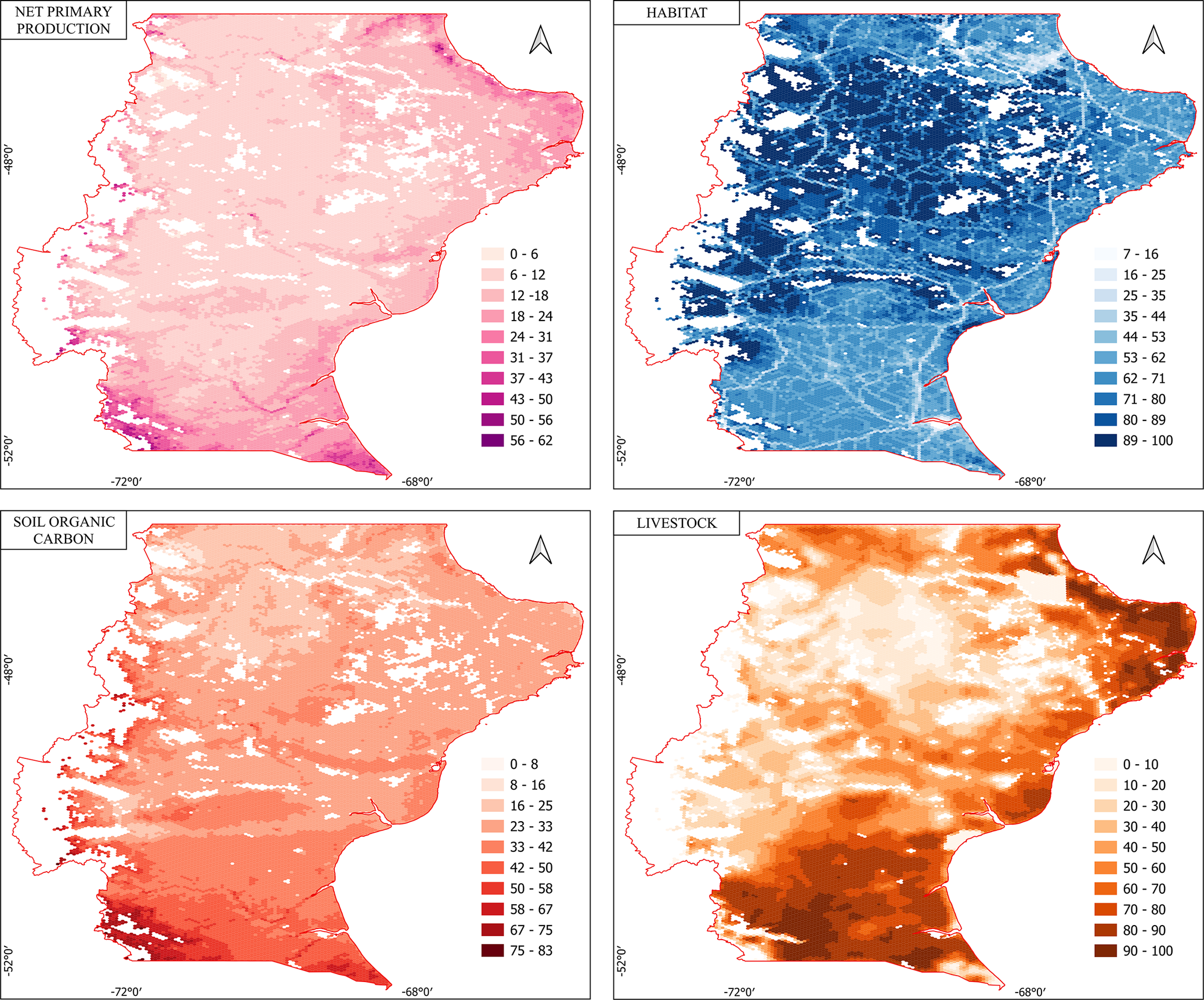
Figure 4. Long description
The layout consists of four maps arranged in a two-by-two grid, each representing Santa Cruz province. Top-left: Net primary production uses a pink to purple gradient, with values from 0 to 62, highest in the south and southeast. Top-right: Habitat provision uses a light to dark blue gradient, values from 7 to 100, with highest values in the north and northeast. Bottom-left: Soil organic carbon uses a light to dark red gradient, values from 0 to 83, highest in the south and southwest. Bottom-right: Livestock provision uses a light to dark orange gradient, values from 0 to 100, with highest values in the south and southeast. Each panel includes a legend with value ranges and a north arrow. Provincial boundaries and main roads are visible as thin lines.
Provisioning ES
Sheep probability (stocking density) fluctuated from 34.3 in Murtillar dwarf-shrubland to 67.4 in the mixed shrubland (Table 3). Variability in sheep production can be attributed to differences in grassland conditions that in turn can be related to NPP variation due to long-term grazing management and climate conditions along vegetation types (Paruelo et al., Reference Paruelo, Golluscio, Guerschman, Cesa, Jouve and Garbulsky2004; Piñeiro et al., Reference Piñeiro, Oesterheld and Paruelo2006). The map of livestock density across Santa Cruz (Figure 4) shows high values in the ecotone between Nothofagus antarctica forest, the grasslands in the west and in the south, and in river valleys and wetlands corresponding to the most productive habitats for livestock production (Peri et al., Reference Peri, Rosas, Rivera and Martínez Pastur2021b). The model of livestock occurrence probability was consistent with the regional/spatial analysis of Peri et al. (Reference Peri, Rosas, Rivera and Martínez Pastur2021b) in which meat production ranged from 0.25 to 0.69 g lamb m−2 yr−1 and greasy wool production from 0.10 to 0.19 g m−2 yr−1. While variation in lamb production was mainly driven by temperature seasonality, NVDI and desertification, the most important variables for explaining variation in greasy wool production were isothermality, temperature seasonality and NVDI (Peri et al., Reference Peri, Rosas, Rivera and Martínez Pastur2021b).
Biodiversity values
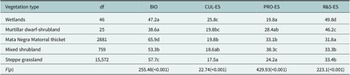
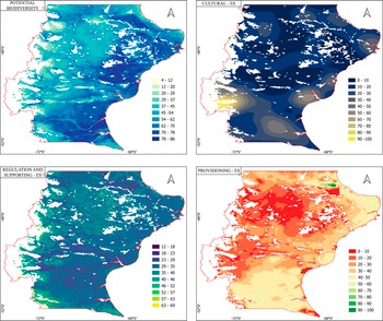
The Mata Negra Matorral thicket showed the highest potential biodiversity compared with other vegetation types (Table 4). Similarly, Peri et al. (Reference Peri, Gaitán, Díaz, Almonacid, Morales, Ferrer, Lasagno, Rodríguez-Souilla and Martínez Pastur2024) reported that the biodiversity was high in shrublands (64.1% in Mata Verde shrublands and 63.7% in mixed shrublands), comparable even to values found in open deciduous forests (N. antarctica forest, with 60.4%). Rosas et al. (Reference Rosas, Peri, Lencina, Lizarraga and Martínez Pastur2022a) determined at the provincial level that mean potential biodiversity showed higher values in shrublands and steppe grasslands in humid areas. The map of potential biodiversity (Figure 5) indicates the lowest values (1–51%) in areas near the mountains and glaciers in the western part of the province. According to Rosas et al. (Reference Rosas, Peri, Lencina, Lizarraga and Martínez Pastur2022a), medium values (52–62%) are observed in the steppe grasslands in the eastern region, while high biodiversity values are primarily concentrated in steppe grasslands located in three distinct geographic locations: the extreme south, the extreme north and the central part of the province. The elevated biodiversity in these three regions may be attributed to landscape heterogeneity, as all three locations exhibit complex geomorphology (e.g. Rosas et al., Reference Rosas, Peri, Martínez Pastur, Peri, Martínez Pastur and Nahuelhual2021a, Reference Rosas, Peri, Lencina, Lasagno and Martínez Pastur2021b, Reference Rosas, Peri, Pidgeon, Martinuzzi, Politi, Pedrana, Díaz Delgado and Martínez Pastur2021c), which may result in a variety of niches and ecotones (Riesch et al., Reference Riesch, Plath and Bierbach2018). This geological complexity may also have hindered the construction of roads in these areas, thereby reducing human access and limiting ecological disturbances within these ecosystems. Consequently, this limited accessibility may have contributed to the higher biodiversity values observed in these specific locations.
ANOVAs for potential biodiversity (BIO), total cultural ecosystem services (CUL-ES), total provisioning (PRO-ES) and total regulating and supporting ecosystem services (R&S-ES) of grasslands and shrublands in Santa Cruz province (Argentina)
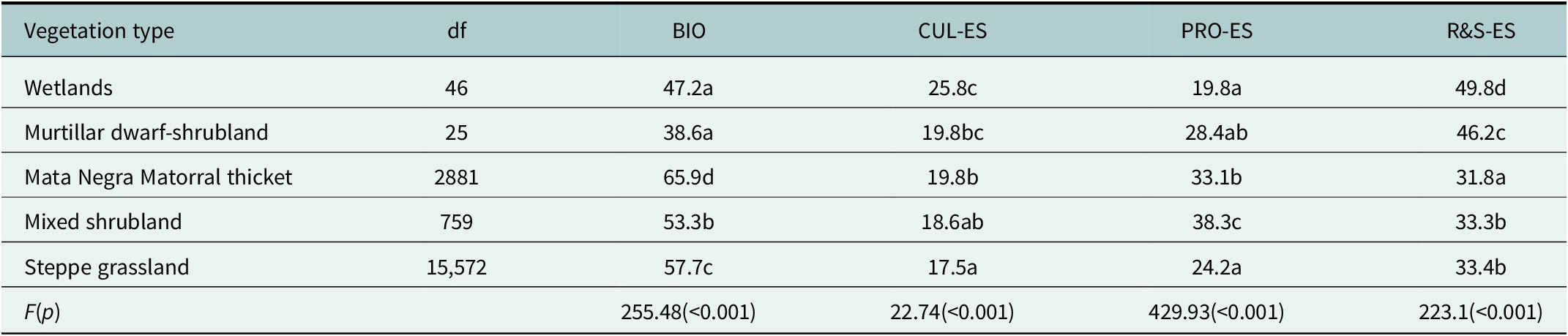
Table 4. Long description
The table has six rows and six columns. Columns from left to right are: Vegetation type, degrees of freedom (df), BIO, CUL dash E S, PRO dash E S, and R and S dash E S. The five vegetation types listed top to bottom are Wetlands, Murtillar dwarf-shrubland, Mata Negra Matorral thicket, Mixed shrubland, and Steppe grassland. For Wetlands, df is 46, BIO is 47.2 a, CUL dash E S is 25.8 c, PRO dash E S is 19.8 a, R and S dash E S is 49.8 d. For Murtillar dwarf-shrubland, df is 25, BIO is 38.6 a, CUL dash E S is 19.8 b c, PRO dash E S is 28.4 a b, R and S dash E S is 46.2 c. For Mata Negra Matorral thicket, df is 2881, BIO is 65.9 d, CUL dash E S is 19.8 b, PRO dash E S is 33.1 b, R and S dash E S is 31.8 a. For Mixed shrubland, df is 759, BIO is 53.3 b, CUL dash E S is 18.6 a b, PRO dash E S is 38.3 c, R and S dash E S is 33.3 b. For Steppe grassland, df is 15,572, BIO is 57.7 c, CUL dash E S is 17.5 a, PRO dash E S is 24.2 a, R and S dash E S is 33.4 b. The last row shows F and p values for each metric: BIO is 255.48 less than 0.001, CUL dash E S is 22.74 less than 0.001, PRO dash E S is 429.93 less than 0.001, R and S dash E S is 223.1 less than 0.001. Numbers range from 0 to 100. Different letters indicate significant differences among vegetation types by Tukey's test at p less than 0.05.
Note: Numbers varied between 0 (minimum provision) and 100 (maximum provision).
F = Fisher’s test, (p) = probability, df = degrees of freedom. Different letters in columns show differences among vegetation types according to Tukey’s test at p < 0.05.
Potential biodiversity and combination maps for cultural, regulating/supporting and provisioning ecosystem services for grasslands and shrublands in Santa Cruz province (Argentina). Numbers varied between 0 (minimum provision) and 100 (maximum provision).
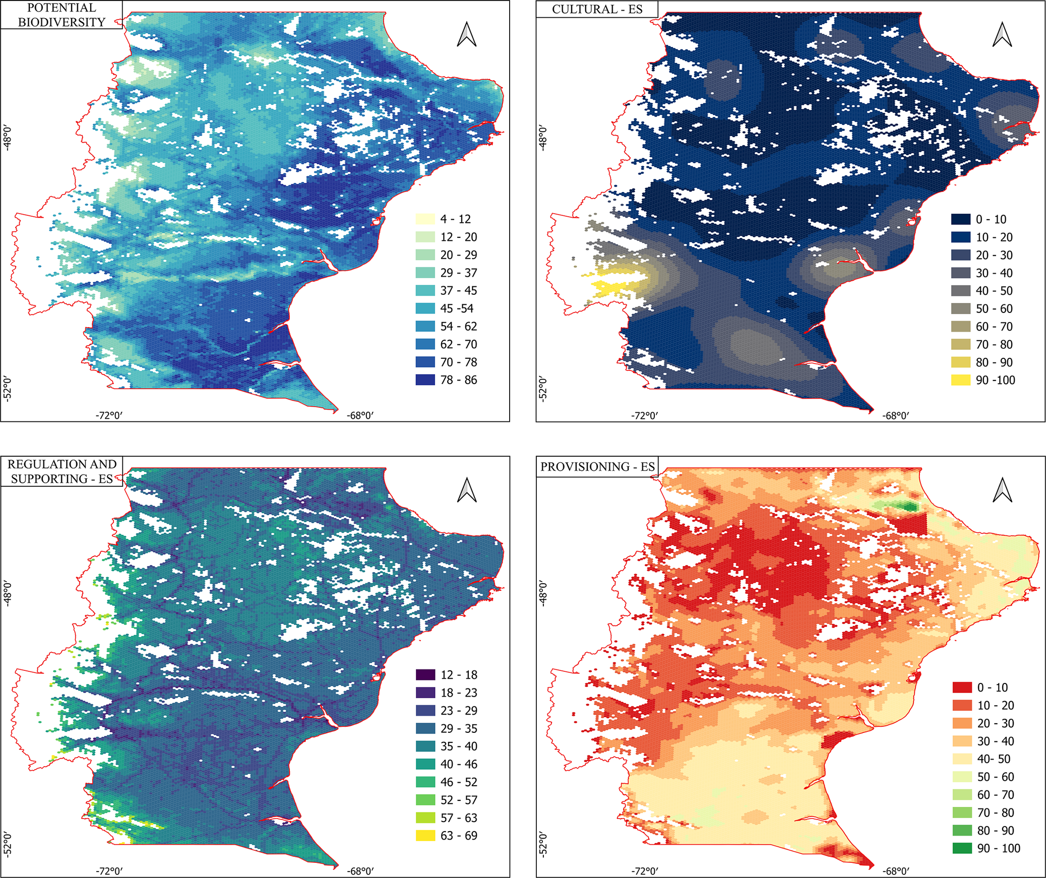
Figure 5. Long description
Top-left panel labeled Potential Biodiversity uses a blue gradient from light yellow (4–12) to dark blue (78–86), with higher values in the northeast and lower in the southwest. Top-right panel labeled Cultural E S uses a gradient from dark blue (0–10) to yellow (90–100), with most of the area in dark blue and isolated yellow patches in the southwest. Bottom-left panel labeled Regulation and Supporting E S uses a gradient from dark purple (12–18) to yellow (63–69), with higher values in the southeast and lower in the northwest. Bottom-right panel labeled Provisioning E S uses a gradient from light yellow (0–10) to dark green (90–100), with high values concentrated in the central and northeast regions and lower values in the southwest. All panels share the same province outline, cardinal direction arrow, and latitude/longitude grid.
Synthesis
The estimates of stocks (e.g. SOC, habitat value) and flows (e.g. NPP, sheep occurrence probability) of natural capital presented in Figures 3 and 4 were integrated to generate maps illustrating three broad categories of ES (cultural, supporting/regulating and provisioning services) and biodiversity values (Figure 5). These synthesis maps reflect the underlying stocks and flows of natural capital that produce ESs, while also highlighting areas where trade-offs and synergies among different ES occur. For example, the total regulating-supporting, total provisioning and total cultural ESs varied with vegetation type (Table 4). While total regulating and supporting ESs, and total cultural ESs were highest in wetlands, total provisioning ESs occurred in mixed shrublands (Table 4). The provision of ESs presented medium values in some shrublands (e.g. Mata Verde shrubland and Murtillar dwarf-shrubland, 43.6–45.3%), and wetlands (47.7%); and minimum values in the other shrubland types (Mata Negra Matorral thicket and mixed shrubland) and steppe grasslands (29.7–30.9%) (Peri et al., Reference Peri, Gaitán, Díaz, Almonacid, Morales, Ferrer, Lasagno, Rodríguez-Souilla and Martínez Pastur2024). The map combining cultural services showed high values associated with the road network and mountainous regions (Rosas et al., Reference Rosas, Martínez Pastur and Peri2022b). Although total cultural ESs are relatively evenly distributed across the province, with low to medium values (less than 30%), total regulating and supporting ESs are most prominent in the western and central parts of Santa Cruz (Figure 5). The very high values for provisioning ESs (Figure 5) observed in the north (>70%) due to oil production, medium values (40–50%) in the south and southwest, areas characterized by more humid grasslands linked to livestock production, are consistent with models reported by Rosas et al. (Reference Rosas, Martínez Pastur and Peri2022b). These results confirmed the hypothesis that the provision of the different ES was not independent of interactions dependent on vegetation types. Also, human activities generate synergies and trade-offs between provisioning ES and biodiversity.
Recommendations for management and conservation
The intensification of land use has demonstrated that optimizing certain ESs, such as provisioning services, is likely to diminish ecological diversity and system stability (Cardinale et al., Reference Cardinale, Duffy, Gonzalez, Hooper, Perrings, Venail, Narwani, Mace, Tilman, Wardle, Kinzig, Daily, Loreau, Grace, Larigauderie, Srivastava and Naeem2012), as well as overall biodiversity (MEA, 2005). In recent years, scientific and policy agendas on biodiversity have shifted to incorporate ES assessments, recognizing the critical importance of monitoring ESs to evaluate the effectiveness of policy frameworks (Liquete et al., Reference Liquete, Cid, Lanzanova, Grizzetti and Reynaud2016; Schwantes et al., Reference Schwantes, Firkowski, Affinito, Rodriguez, Fortin and Gonzalez2024).
The spatial analysis of ESs and biodiversity values presented here further emphasizes that the benefits derived from nature extend far beyond the direct supply of provisioning services such as fuel, food and fiber. Notably, the observed spatial overlaps and mismatches between the supply and demand for different categories of ESs, namely cultural, regulating/supporting and provisioning services, highlight both opportunities and challenges for integrating ES considerations into land use and biodiversity planning. For instance, areas with high biodiversity in the north, center and south of the province also serve as key regions for regulating services, making the development of land management strategies to secure both in these zones relatively straightforward. Conversely, for services like provisioning and cultural services, which are both closely linked to road access, more detailed analyses of value, potential trade-offs and associated costs for conservation or enhancement may be necessary.
Final remarks and conclusions
The findings of this study provide valuable insights for land use planning in Santa Cruz, integrating considerations of ESs and biodiversity values. With the recent increase in tourism, cultural ESs have gained greater prominence (Martínez Pastur et al., Reference Martínez Pastur, Peri, Lencinas, García Llorente and Martín López2016a) and could play a key role in the sustainable exploitation of the region’s natural capital. Nonetheless, traditional activities such as livestock production remain vital, especially for the intangible cultural ESs, including local identity and cultural values. A significant challenge lies in reconciling the need to maximize provisioning services, which are closely linked to cultural identity, while preserving the capacity of the steppe grasslands to continue providing regulating and supporting services (Ahtikoski et al., Reference Ahtikoski, Tuulentie, Hallikainen, Nivala, Vatanen, Tyrväinen and Salminen2011).
Implementing adaptive grazing management, with stocking rates aligned to forage availability and net primary production, may yield more sustainable long-term economic benefits without degrading the steppe grasslands or compromising the natural capital that contributes to human well-being through cultural ESs such as ecotourism and the Patagonian sense of place. In this context, sustainable land management, particularly regarding grazing practices, must incorporate the consideration of other ESs, especially the regulating and supporting services, into management plans. One strategy is to maintain high levels of biodiversity within managed ecosystems, which might positively influence provisioning ESs (Duru et al., Reference Duru, Therond, Martin, Martin-Clouaire, Magne, Justes, Journet, Aubertot, Savary, Bergez and Sarthou2015; Duarte-Guardia et al. Reference Duarte-Guardia, Peri, Martinez-Pastur, Lasagno, Lencinas, Thomas and Ladd2024). Preserving heterogeneity at the landscape scale might also enhance ecosystem resilience and stability in response to global environmental change drivers (e.g. Geijzendorffer and Roche, Reference Geijzendorffer and Roche2013).
A thorough understanding of the processes underlying ES supply, as well as the trade-offs with biodiversity conservation, is a valuable tool to support spatial planning and land management decisions (Carvalho Santos et al., 2015).
Enhanced decision-making in land management necessitates empirical data on the effects of landscape-scale conservation approaches on trade-offs between biodiversity and ESs (Cordingley et al., Reference Cordingley, Newton, Rose, Clarke and Bullock2016). Our findings underscore opportunities to integrate biodiversity conservation with the preservation of ESs. The trade-offs identified in this analysis represent areas where further research could deepen understanding and potentially contribute to the development of more effective management strategies.
Open peer review
For open peer review materials, please visit http://doi.org/10.1017/dry.2026.10038.
Data availability statement
Data are available from the institutional repository at https://repositorio.inta.gob.ar/
Author contribution
Data Curation: P.L.P., R.L., M.V.L., J.R-S., G.M.P.; Funding Acquisition: P.L.P.; Investigation: P.L.P., R.L., M.V.L., G.M.P.; Supervision: J.R-S.; Visualization: P.L.P.; Writing – Editing, Methodology: B.L., M.V.L., J.R-S., Writing – Original Draft Preparation, Review and Editing: P.L.P., G.M.P.
Financial support
This research was supported by Proyecto Estructural Macroregional Gestión Sostenible de los sistemas forestales naturales y cultivados para el desarrollo de los territorios y la provisión de los servicios ecosistémicos en Patagonia Andina (Código: 2023-PE-L03-I033).
Competing interests
The authors declare that they have no competing interests.


 Open access


Comments
Río Gallegos, 19 November 2025
Editor Cambridge Prisms: Drylands
Dear Editors
I send you the manuscript Ecosystem service and biodiversity values in grassland and shrublands in Santa Cruz province (Argentina) (Pablo L. Peri, Romina Lasagno, Brenton Ladd, María V. Lencinas, Julián Rodriguez-Souilla and Guillermo Martínez Pastur) to be considered in the journal Cambridge Prisms: Drylands in the forthcoming Themed Collection entitled “Drylands of South America: Ecology without borders that integrates environment and society”. I confirm that neither the manuscript nor any parts of its content are currently under consideration or published in another journal.
We believe that this manuscript provides new information related to integrate monetary values of provisioning ecosystem services (ES) with other non-monetary ES and biodiversity for human well-being in grasslands of Southern Patagonia.
Yours sincerely
Dr. Pablo PERI
UNPA-INTA-CONICET
cc 332 (CP 9400), Río Gallegos, Santa Cruz, Argentina
Email: peri.pablo@inta.gob.ar
Ph/FAX : +54-2966-442305