

1. Introduction
Given the recent advances in data science, aided by a rapid expansion in computing power, the health and care (H&C) actuarial field is experiencing a transformation. Actuaries are well positioned to leverage the increasing variety and volume of internal and external data to aid decision-making and strategic planning. Since 2018, the Institute and Faculty of Actuaries (IFoA) has increased its focus on data science, including formation of various working parties and the inclusion of data science in qualifications (Marshall, Reference Marshall2024). For the purpose of this paper, we defined data science as an umbrella term for any field of research that involves the processing of large amounts of data in order to provide insights into real-world problems (The Alan Turing Institute, 2025). Although not a new area of work for actuaries, the wider fields of data science showcase many new techniques.
This document presents a structured framework to guide H&C actuaries in selecting data science techniques appropriate for a project and aids in systematic, well documented decision making and reporting. Throughout a data analysis project, both explicit and implicit analytics decisions are made, such as defining the scope of the project and underlying data, selecting features, and choosing model class and parameters. The checklist provided in this framework (see Table 1) offers a comprehensive overview of these decisions, ensuring that no aspect is overlooked or omitted in the analytical and reporting process.
Framework checklist

We have aimed to make this framework accessible to a broad audience. However, we recognise that some sections, such as those on encoding categorical features and on gradient boosting machines (GBMs), may be challenging to those new to the field. To this end, we have included references for further reading as well as specific examples to illustrate various scenarios a health and care actuary might encounter. The examples weigh the strengths and weaknesses of different methodological approaches and provide guidance on their appropriateness under varying circumstances.
2. Developing the Framework
The IFoA working party “Techniques in Data Science in Health and Care” contains a mix of actuaries, data scientists, epidemiologists and healthcare professionals. This group was tasked with developing an index of the data science (or closely related) aspects of H&C actuarial data analytics projects that utilise tabular data. The scope was restricted to tabular data since traditional actuarial analysis, such as experience analysis, is based on tabular data. This index was then grouped into four categories:
-
(a) Study design and technology requirements
-
(b) Pre-model
-
(c) Model
-
(d) Post-model
From this grouped index, a checklist was developed and reviewed within the working party (see Table 1). Each item included in the checklist contains a summary (Section 3) and, where relevant, key references for further reading. Generative AI including large language models are considered out of scope. Although generative AI can play a role in analysis of tabular data, for example by suggesting code, brainstorming and even imputation of missing data, their use in traditional actuarial analysis is currently limited.
Various documents including the Technical Actuarial Standard 100 (Financial Reporting Council, 2023) and the STrengthening the Reporting of OBservational studies in Epidemiology (STROBE statement) were also consulted improve the framework’s comprehensiveness (von Elm et al., Reference von Elm, Altman, Egger, Pocock, Gøtzsche and Vandenbroucke2007).
3. The Framework
3.1. Research Question
High quality research is underpinned by a good research question. Therefore, it is important to invest time in defining the research question to be answered. It can be difficult and time-consuming to revisit the question after analytics have been performed, therefore consultation and agreement with key stakeholders at the start is vital. The purpose and scope of the investigation should be well-defined and documented.
The acronym “FINER” can support defining a good research question (Hulley et al., Reference Hulley, Cummings, Browner, Grady and Newman2007): feasible, interesting, novel, ethical, relevant (see Table 2).
An adapted version of the FINER criteria for a good research question and project plan (Hulley et al., Reference Hulley, Cummings, Browner, Grady and Newman2007)

3.2. Analytical Project Categorisation
Analytic projects undertaken by actuaries are typically observational in nature, relying on pre-existing data rather than introducing treatments or interventions (e.g. clinical trials). In clinical literature, analytical projects are referred to as “studies” and there are three main classes of observational study designs available for H&C data (Mann, Reference Mann2003). Each study design offers specific strengths and weaknesses that are extensively covered in epidemiological literature. Here we look at the three types of observational data study in more detail.
3.2.1. Cohort Studies
H&C actuaries are likely familiar with cohort studies, where a cohort of people or policies is followed over time, as this is the default study design for experience analysis of an insurance portfolio. Cohort studies are useful for studying incident cases and establishing causal relationships. For most actuarial cohort studies, exposure data is collected prospective to an outcome of interest, which reduces potential recall bias. Recall bias typically occurs when exposure is collected retrospective to the outcome. For example, an individual may be more or less likely to recall the risk factors they were exposed to after they experience an outcome of interest. When the outcome of interest is rare, these studies require progressively larger cohorts and longer follow-ups to ensure sufficient statistical power (Section 3.6). An example of a cohort study is following a cohort of people over time to compare lung cancer incidence rates between smokers and non-smokers.
3.2.2. Case Control Studies
Case-control studies are more efficient study designs for rare outcomes or where follow-up time is limited. Case-control studies compare individuals with a particular outcome (cases) to those without it (controls) to analyse potential risk factors. Unlike cohort studies, there is no follow-up or exposure time. Case-control studies are efficient but suffer from various potential biases (e.g. recall bias), especially when data is retrieved retrospective to the outcome. An example of a case-control study is a study comparing fraudulent claims (cases) to genuine claims (controls) to identify predictors of fraudulent claims.
3.2.3. Cross-Sectional Studies
Cross-sectional studies are observational studies that analyse data on exposure and outcome from a population at a single point in time. Cross-sectional studies can analyse the prevalence of a condition, but not the incidence, due to the lack of a temporal element. For this reason, cross-sectional studies are useful for demographic distributions and outcomes where the individual remains within the data set to be observed (such as low mortality diseases like diabetes). Cross-sectional studies are not useful for high mortality conditions such as stroke since, at any given time, the number of prevalent cases will be low. An example of a cross-sectional study is an analysis of life insurance policy ownership by socioeconomic status.
Note that interventional study designs (clinical trials) and descriptive study designs (case reports, case series and ecological studies) are out of scope of this framework as these study designs are generally not useful for actuarial projects.
3.3. Reproducibility
Reproducibility of findings is the cornerstone of scientific research. This issue is particularly relevant for H&C actuaries who rely on predictive modelling and statistical analyses to inform decision-making. Reproducibility in the narrow sense (i.e. on the same data set using the same methods) ensures that findings are consistent and trustworthy and enables peer-review. Epidemiological research, which includes most analytical work by H&C actuaries, is considered reproducible when requirements around data, methods and documentation have been met (Peng et al., Reference Peng, Dominici and Zeger2006).
3.3.1. Reproducible Data
Ensuring reproducible data involves maintaining consistent data sources, documenting pre-processing steps, and storing both raw and processed data sets in repositories accessible to internal reviewers. Techniques such as data versioning, hashing for integrity checks, and structured metadata (e.g., using Findable, Accessible, Interoperable and Reusable (FAIR) principles as per Wilkinson et al., Reference Wilkinson, Dumontier, Aalbersberg, Appleton, Axton, Baak, Blomberg, Boiten, da Silva Santos, Bourne, Bouwman, Brookes, Clark, Crosas, Dillo, Dumon, Edmunds, Evelo, Finkers, Gonzalez-Beltran, Gray, Groth, Goble, Grethe, Heringa, ’t Hoen, Hooft, Kuhn, Kok, Kok, Lusher, Martone, Mons, Packer, Persson, Rocca-Serra, Roos, van Schaik, Sansone, Schultes, Sengstag, Slater, Strawn, Swertz, Thompson, van der Lei, van Mulligen, Velterop, Waagmeester, Wittenburg, Wolstencroft, Zhao and Mons2016) help ensure that analyses can be replicated by colleagues under identical conditions.
3.3.2. Reproducible Methods
Version control tools such as Git enable actuaries to maintain an audit trail of the code base, revert to earlier analysis stages, systematically review model changes over time and facilitate collaborative workflows. Git can also support data lineage tracking by indexing data pre-processing.
Randomness in data science methods (e.g. tree-based models, neural networks, clustering algorithms, bootstrapping and cross-validation) can be controlled by setting a random seed. Despite this, fixing a seed does not guarantee full reproducibility due to variations in hardware and software dependencies, underscoring the importance of containerisation tools like Docker or virtual environments for computational consistency. For these reasons, it is also best practice to document the software environment and package versions used.
Model and workflow ownership, as per TAS 100 (Financial Reporting Council, 2023), also supports reproducibility by having a clear point of contact available for queries.
3.3.3. Reproducible Documentation
Well-structured workflows and comprehensive documentation support reproducibility. This includes using programming tools such as R Markdown and Jupyter Notebook that integrate code, output and explanatory text; including documentation around key decisions made during data pre-processing and analytics, into a single shareable document.
3.4. Data Selection
3.4.1. Data Selection Criteria
Well-designed studies include data selection criteria that define which subjects should be included and excluded. Data selection criteria should be defined to ensure appropriateness of the data. Important criteria involve geographical region, date of birth, commencement year (of insurance policy), calendar years of follow-up and medical history. Failure to specify data selection criteria can result in non-representative or irrelevant study participants. For example, when using external data sets such as a data set from the Continuous Mortality Investigation (CMI), actuaries should take care to understand the underlying selection rules used by the original data collectors, such as the exclusion of rated lives in analyses of standard-term assurances.
Data selection criteria vary by study design as cohort studies and cross-sectional studies enrol subjects based on an exposure (such as a hospital visit or being a policy-holder), while case-control studies enrol subjects based on an outcome (such as a fraudulent claim).
3.4.2. Data Bias
Data bias may arise from inherently biased data sampling methods, historical bias within the data (including bias due to over-representation of certain groups) and/or omission of key predictive attributes from the data (Financial Reporting Council, 2024).
Data bias can arise from various factors, examples are:
-
1. Anti-selection, where individuals with poorer health or pre-existing conditions are more likely to buy or retain coverage.
-
2. Data drift, where the statistical distributions of input features change over time. For example, the BMI distribution changing over time and the proportion of smokers decreasing over time.
-
3. Concept drift, where the relationship between an input feature and the outcome changes by issue year. For example, inflation affects the relationship between sum assured and outcomes over time and improvements in underwriting could affect the impact of duration on outcomes.
-
4. Reporting bias where not all data is captured consistently or accurately. For example, underreporting of smoking in the data set.
-
5. Outcome definition bias, where outcome definitions (e.g. ICD-11 codes), or even conditions covered can change over time.
-
6. Omission of key predictive features, where key predictive features are missing from the data. For example, if smoking is not captured in a life insurance claim analysis, part of the effect of smoking could be assigned to features correlated with smoking such as males and low sums assured.
Mitigating data bias often requires bespoke solutions and can be adjusted for within a model or data set. For example, sum assured can be inflation-adjusted in historic data. Various strategies including up-sampling and weights can be considered (Section 3.12) to deal with data drift, and data selection criteria can also be utilised to deal with data bias, for example by excluding unreliable or non-representative data. Section 3.5 discusses some techniques in identifying unreliable or non-representative data.
3.4.3. Ethical and Privacy Controls
Actuaries should ensure that all data sets comply with relevant data protection regulation including UK GDPR (Regulation (EU) 2016/679, 2016) and the Data Protection Act 2018. Data collection and use should also comply with ethical approval and participant consent, where appropriate. Additionally, data analytics projects will be subject to internal governance processes, including legal, regulatory and audit requirements, as well as internal risk management guidance and professional guidance such as TAS 100 (Financial Reporting Council, 2023). The regulatory landscape is subject to constant change. For example, whilst direct use of protected characteristics is widely prohibited, indirect discrimination by proxy variables or complex algorithms is currently a regulatory grey area (Xin & Huang, Reference Xin and Huang2024). Therefore, actuaries are encouraged to keep up to date with regulatory developments.
Advanced algorithms and big data may elevate privacy risks and inadvertent use of protected characteristics by proxy. Structured ethical checkpoints throughout the analytics project (problem definition, data, modelling, evaluation and deployment), as discussed in recent actuarial literature (Huang, Reference Huang2025) may help guard against these risks. These checkpoints help embed principles such as accountability, transparency and privacy. Transparency is further aided by model explainability (Section 3.15). Bias and fairness are further covered in Section 3.14.6.
3.5. Data Cleaning
Effective checks and controls should be applied to the data and any material bias should be identified (Financial Reporting Council, 2023). Checks and balances include:
-
• Data quality checks to identify any structural (3.5.1) or content issues (3.5.2)
-
• Consistency checks, including statistical checks (3.5.3).
All checks and controls that have been applied to the data should be documented (Financial Reporting Council, 2023).
3.5.1. Structural Issues
Structural issues include duplicated rows, columns and lives, incorrect variable types, and redundant columns that can introduce inefficiencies and distort analytical outcomes. Duplicated rows may arise from data entry errors or merging data sets, leading to overrepresentation of certain observations. Duplicated lives can arise from a claim by the same person on multiple policies, or tranches of the same policy. Similarly, redundant columns, often created during data processing, can add unnecessary complexity without providing additional information.
Incorrect variable types, such as numerical values or dates stored as text, can interfere with calculations and statistical modelling as well as visualisations. Addressing these structural issues early prevents downstream errors and improves data integrity. Automated scripts and validation checks can help identify and correct such problems efficiently.
3.5.2. Content Issues
Content issues in data cleaning include missing data and outliers as well as inconsistent and implausible data. Outliers can be identified by visualising histograms or performing range checks, but their interpretation depends on context. For instance, in lab tests and biometrics, outliers can be due to different units (e.g. mmol/L vs. mg/dL for cholesterol levels), or system conversions (imperial versus metric). In financial data sets, negative values can indicate refunds rather than errors. Addressing outliers or missing data ideally involves identifying their root cause (e.g. by speaking with the data supplier) before determining whether correction, transformation, flooring/capping or exclusion is appropriate.
Missing data can be missing completely at random (MCAR), missing at random (MAR) and missing not at random (MNAR) (Mack et al., Reference Mack, Su and Westreich2018).
-
1. MCAR occurs when missingness is unrelated to any observed or unobserved variables. An example of this is a batch of policy holders missing smoking information due to a data entry error. Although statistical power is reduced, there is no introduction of bias into the analysis.
-
2. MAR occurs when missingness is systematically related to observed, but not unobserved data. For example, younger (observed) policyholders being less likely to disclose smoking habits. MAR can introduce bias if not properly adjusted for but can often be corrected for.
-
3. MNAR occurs when missingness is related to unobserved factors. For example, high-risk (unobserved) individuals omitting disclosure of health conditions. MNAR is most problematic since it cannot be corrected for since the factors influencing missingness are unobserved. MNAR is most likely to introduce bias in any subsequent model.
Dealing with outliers and missing data requires a tailored approach, as these issues are often non-random and can introduce bias if mishandled. One common solution, imputation, involves replacing missing values (or outliers) using statistical or machine learning techniques in order to retain useability for analysis or modelling. Simple imputation methods, such as replacing missing values with the mean or median, can distort distributions and weaken predictive models. Multiple imputation by chained equation (MICE) (White et al., Reference White, Royston and Wood2011) has traditionally been regarded as the gold standard for imputation of missing data. Recently, various more sophisticated techniques utilising tree-based models such as missForest are available and have been outperforming MICE in certain studies (Luo, Reference Luo2022; Waljee et al., Reference Waljee, Mukherjee, Singal, Zhang, Warren, Balis, Marrero, Zhu and Higgins2013). Imputation may not produce reliable results after a certain threshold of missingness is met. Unfortunately, this threshold is highly dependent upon type of missingness and is specific to each data set. For categorical features (e.g. smoking status) a simple solution can be to introduce a new category: “unknown.” Should different types of missingness (e.g. blank values vs. missing values) be present, these should be considered separately as these could represent different underlying issues.
3.5.3. Data Consistency Checks
Various types of consistency checks can be considered (see Table 3).
Consistency checks classes

3.6. Data Sufficiency and Reliability
3.6.1. Credibility
Credibility is the weighting of different estimates to come up with a combined estimate. Generally, credibility combines observed experience with a more stable, yet less individualised estimate (i.e. the a priori assumption). Credibility is especially useful when observed data is limited or volatile, which may result in unreliable model predictions. Traditionally, limited fluctuation (LF), greatest accuracy (GA) and Bayesian methods have been used for credibility (Atkinson, Reference Atkinson2019). More recently, LASSO and random effects models allow for credibility to be integrated within the model itself.
3.6.1.1. Limited fluctuation
Limited Fluctuation (LF) is widely used by H&C actuaries due to its simple application. There are various drawbacks for LF (Atkinson, Reference Atkinson2019) including the arbitrary setting of values that determine full credibility, the assumption of a fully credible prior and the square root formula reaching full credibility prematurely. LF is underpinned by the normal approximation to the Poisson, whose assumptions could be violated (e.g. by overdispersion or zero inflation as shown in Section 3.10.3). Additionally, LF may significantly underestimate credibility for populations with exceptionally light mortality experience (Gong et al., Reference Gong, Li, Milazzo, Moore and Provencher2018).
3.6.1.2. Greatest accuracy
The GA theory (also known as Bühlmann credibility) produces a credibility-weighted rate that blends the observed rate and a portfolio rate using parameter z (the credibility weighting). Note this is different from LF, which blends the observed rate with a prior rate.
The GA method is statistically more robust than LF but requires a portfolio of data from comparable risk groups, which means in practice it is seldom used by H&C actuaries. GA may produce a poor approximation when the random variable has a heavy tail (Atkinson, Reference Atkinson2019).
3.6.1.3. Shrinkage-based credibility models
Contrary to LF and GA, shrinkage-based models allow for multivariate credibility using regression formulae:
-
• Generalised Linear Models (GLMs) are not suitable for credibility since GLMs do not apply shrinkage (unless extended) and incorporate uncertainty into confidence intervals, p-values etc. However, three model classes, Bayesian models, random effects models and penalised regression models incorporate some form of shrinkage, similar to credibility.
-
• Bayesian methods allow for the explicit incorporation of a prior into a model, allowing for updating a prior based on new experience, like credibility.
-
• Random effects models shrink individual estimates towards a group mean and pure random effects models have been shown to be equivalent to Greatest Accuracy credibility (Nelder & Verrall, Reference Nelder and Verrall1997).
-
• Penalised regression models can shrink regression coefficients, effectively incorporating credibility (Casotto et al., Reference Casotto, Banterle and Beraud-Sundreau2023).
3.6.2. Sample Size Calculation
When applying for access to certain health and care data sets, sample size calculations may be required by ethics committees to ensure studies are robust and well-designed.
Sample size calculations prevent unreliable, inconclusive, and non-reproducible results as well as reduce the risk of false negative results (Ioannidis, Reference Ioannidis2005). This is similar to actuarial credibility theory -where a data set must reach a certain size before we can rely on observed experience rather than external assumptions. Sample size calculations may not be relevant for actuarial projects where the objective is to extract the maximum number of insights from a data set, or for pricing exercises.
Sample size calculations require (Sharma et al., Reference Sharma, Mudgal, Thakur and Gaur2020):
-
• A null hypothesis and alternative hypothesis
-
• Acceptable significance level (the probability of incorrectly rejecting the null hypothesis), typically set at 5%
-
• Study power (the probability of correctly rejecting the null hypothesis), typically set at 80%
-
• Expected effect size, typically expressed as a relative risk, odds ratio or hazard ratio
-
• Underlying event rate in the population
-
• Margin of error
-
• Standard deviation in the population
-
• A one tail and two tail inferential statistical test
-
• A design effect
3.7. Data Partitioning
Machine learning models can learn from greater granularity, opening the risk of overfitting the data. Overfitting occurs when a model learns not only the underlying patterns in the training data but also the noise, resulting in poor performance on new, unseen data. To reduce overfitting, it can be good practice to split data into testing and training data. Sometimes a third group, validation data, is also used. Training data is used for fitting models, validation data for calibrating and evaluating models during development, and the test data (sometimes called holdout data) is used for evaluating final models. Certain models, such as gradient boosting, can track performance on the test data, whilst fitting on the training data, and stop once performance on the test data starts deteriorating. To further guard against overfitting and improve generalisation to new data, cross-validation can be used. Cross-validation goes beyond a single test-train split by dividing the data into multiple subsets (or “folds”) and cycling through them to train and test the model. Stratifying data splits and folds by important features (e.g. age groups) or by the outcome class (e.g. claims) can help reduce variation between splits and folds and lead to more reliable model evaluation and selection.
A particular pitfall in test-train splits is data leakage, where information about the test data set unintentionally ends up in the training data set, resulting in overly optimistic model performance. An example of data leakage is imputing missing data using the entire data set. For example, using average sum assured across the entire data set (test and training) to impute missing values. This imputation leaks information from the test data set (that will be used for model evaluation) into the training data set. Therefore, any subsequent model may learn patterns that reflect the test data distribution rather than the underlying relationship between sum assured and outcome (e.g. claims). The contaminated sum assured values may result in overly optimistic model performance on the test data, relative to performance on truly unseen data.
3.8. Candidate Features
Candidate features are those variables initially considered for model development. Some features are excluded for non-predictive reasons, such as regulatory constraints, ethical considerations (avoiding discriminatory variables), domain knowledge (elimination of a feature due to inconsistent recording) or data quality issues (incomplete or unreliable data). These external factors constrain variable selection before any predictive assessment begins.
Next, the feature selection process (Section 3.11) evaluates the remaining features for their predictive ability on the target variable. For example, if the sum assured was algorithmically dropped by stepwise AIC after income level and credit score have been included, these socioeconomic factors may well be the underlying drivers and not the sum assured itself.
We also recommend documenting excluded features along with the main reasons for exclusion. This level of transparency can ensure complying with regulations and preserving valuable “negative findings” that may be useful for future model refreshes (Ioannidis, Reference Ioannidis2005). It also helps with proper model interpretation, makes modelling decisions more understandable to stakeholders, and supports future model validation and refinement.
In addition to features used in the final model, it could be valuable to consider features that ultimately cannot be used for pricing or decision making. For example, considering policy commencement year and birth year can prevent cohort effects incorrectly getting assigned to other features. For instance, if underwriting standards have recently improved dramatically, this is a policy commencement year effect. Without considering policy commencement year, the effect could be incorrectly assigned to policy duration.
3.9. Feature Engineering
Feature engineering is the process of creating new variables or transforming existing ones from raw data for a model. Variables can also be called “input features.” This often involves generating new data fields using existing information. Feature engineering techniques can be split into three categories: feature engineering for numeric features (including dates), categorical features (e.g. region or gender) and variable interactions (e.g. combining age and smoking status to model risk more effectively).
3.9.1. Numeric Features
Numeric feature engineering involves transforming numeric variables (both discrete and continuous) to better capture their relationships with the target variable. Since relationships between predictors and outcomes are rarely perfectly linear in real-world data, these transformations are critical for improving model performance, especially for linear models, including GLMs and their regularised variants, such as Ridge, Lasso and Elastic Net.
Typically, the process begins with an exploratory data analysis to understand the distribution of each numeric feature and its empirical relationship with the target variable. Visualisations such as scatter plots and density plots can help with deciding if any transformation is required. For instance, logarithmic transformations may be useful for features with significant skewness, whilst non-linear relationships with the target may justify including additional polynomial terms. The principal methods of transforming numeric features are listed in Table 4.
Overview of feature engineering methods for numeric features

Unlike linear models, most machine learning models such as neural networks and tree-based models can discover non-linear relationships on their own without explicit transformation. But feature engineering is still important because the model performance can still depend on how the input data is represented (Goodfellow et al., Reference Goodfellow, Bengio and Courville2016). Particularly for neural network models, the likelihood of convergence is higher and the rate of convergence is faster during model training when all features are standardised. A popular way of doing this is Z-score normalisation (LeCun et al., Reference LeCun, Bottou, Orr, Müller, Orr and Müller1998b), where
 $${z_i}$$
is the normalised version of the original feature
$${z_i}$$
is the normalised version of the original feature
 $${x_i}$$
,
$${x_i}$$
,
 $${\mu _i}$$
is the mean of
$${\mu _i}$$
is the mean of
 $${x_i}$$
and
$${x_i}$$
and
 $${\sigma _i}$$
is the standard deviation of
$${\sigma _i}$$
is the standard deviation of
 $${x_i}$$
:
$${x_i}$$
:
 $${z_i} = \;{{{x_i} - \;{\mu _i}} \over {{\sigma _i}}}$$
3.9.2. Categorical Features
Categorical features are not ingested by most models and require encoding into numeric values. The default is often dummy encoding, or one-hot encoding. Both dummy encoding and one-hot encoding generate binary columns for each of the categories. Contrary to one-hot encoding, dummy encoding drops one category to avoid issues with multicollinearity in linear models (the dropped category becomes the intercept or baseline). These encodings are problematic with high-cardinality features because of the numerous columns created that increase the risk of overfitting to training data and model training computational resources. This problem is exacerbated further when variable interactions (Section 3.9.3) are allowed, whether done automatically by the model or manually by domain experts. To mitigate this issue, dimensionality reduction techniques such as PCA can be used post-categorical encoding to condense the full feature set into orthogonal principal components.
More sophisticated encoding techniques can be used to transform a categorical column into a dense numeric feature. For instance, target encoding can be used by mapping each category to the average value of the target variable (Section 3.10.2). However, using this method naively can cause data leakage (Section 3.7), which in turn leads to overfitting to the training data. An effective means of reducing data leakage is to apply cross-validation on target coding of each categorical variable, as shown in Figure 1. For unseen data, the target encoded values are based on the entire training data set.
How to incorporate cross-validation into target encoding to prevent data leakage in training data with 3 random folds.

Categorical embedding provides an alternative to target encoding by isolating the individual effect of each category. This technique is widely used in Natural Language Processing (NLP), in which words are converted into dense numeric vectors with considerably fewer dimensions than one-hot vectors. Word embeddings are learnt by training neural networks on tasks like predicting context words (Mikolov et al., Reference Mikolov, Chen, Corrado and Dean2013). In a similar fashion, categorical embeddings can be trained on prediction tasks. The resulting model’s coefficients assigned to each category will become its numeric representation.
Some ML models do not need a separate procedure to encode categorical features, as they can natively encode those features. Examples of these kind of models are CatBoost (Prokhorenkova et al., Reference Prokhorenkova, Gusev, Vorobev, Dorogush and Gulin2018) and LightGBM (Ke et al., Reference Ke, Meng, Finley, Wang, Chen, Ma, Ye and Liu2017). Also, grouping rare or similar categories together decreases cardinality and reduces overfitting. The cost of grouping, however, is reduced granularity that may result in losing valuable information differentiating the original categories. Grouping can be performed either manually with domain knowledge or automatically with unsupervised learning techniques like K-means.
3.9.3. Feature Interactions
Feature interaction happens when the influence of a feature on the target variable relies on the values of other features. In these instances, the combined effect cannot be isolated by individual features.
Most machine learning models can automatically learn feature interactions. This includes tree-based models and neural network models. On the other hand, models traditionally used by actuaries are those that can be represented explicitly using a regression formula, or more generally speaking, have an additive structure:
 $$g\left( {E\left[ y \right]} \right) = \;{\beta _0} + \sum {f_i}\left( {{x_i}} \right)$$
, where
$$g\left( {E\left[ y \right]} \right) = \;{\beta _0} + \sum {f_i}\left( {{x_i}} \right)$$
, where
 $$E\left[ y \right]$$
is the expected value of the target variable,
$$E\left[ y \right]$$
is the expected value of the target variable,
 $$g$$
is the link function and
$$g$$
is the link function and
 $${x_i}$$
is a feature. These two model classes represent two distinct modelling cultures, which are discussed in Section 3.10.1.
$${x_i}$$
is a feature. These two model classes represent two distinct modelling cultures, which are discussed in Section 3.10.1.
A main drawback of using additive models is that interaction terms need to be explicitly defined. Construction of these interaction terms used to be a cumbersome, time-consuming process requiring deep domain expertise. However, with the advancement of data science, an automated way of developing additive models is to (Tam & Luteijn, Reference Tam and Luteijn2025):
-
1. Create a baseline model that contains just individual effects;
-
2. Employ GBMs to identify interaction effects by training the model to predict residuals
-
3. Include the interaction terms and retrain the additive model
An interaction term most H&C actuaries are familiar with is the interaction between smoking status and age in relation to mortality. Figure 2 shows the expected term assurance mortality rates by policyholder age across all genders and durations (Continuous Mortality Investigation, 2021), splitting between those underwritten as smokers and non-smokers. The relative mortality of smokers compared to non-smokers increases with age up to around the 80s, after which it begins to decline slightly. Therefore, the smoker excess mortality risk by age cannot be captured by a single loading.
CMI expected term assurance mortality rates by age: smokers (orange) versus non-smokers (blue) (all genders, all durations; authors’ analysis).

3.10. Model Design
Model selection matters since various model types (e.g. GLMs and tree-based models) have different strengths and weaknesses in terms of predictive performance, transparency, interpretability, logistics and stakeholder trust. Model selection should align with the intended use of the model. For example, a pricing model may require more transparency due to regulatory requirements and explanation to senior management, whilst an operational model aimed at improving processing efficiency may have an alternative internal business priority such as speed and predictive accuracy over transparency.
We assume familiarity with traditional models such as GLMs. This section will cover data science methods that can be layered on top of models (such as regularisation and ensemble modelling) and less traditional models (gradient boosting and neural networks).
It is important to ensure actuaries understand the models used, including intended use and weaknesses. Lack of full understanding leaves actuaries open to model risk, defined in TAS 100 as
The risk that models are either incorrectly implemented (with errors) or make use of assumptions that cannot be justified rigorously, or assumptions that do not hold true in a particular context (Financial Reporting Council, 2023).
An important distinction in model types is between additive models that require a regression formula (e.g. GLMs) and models that learn their structure automatically such as tree-based models and neural networks. This distinction was described by Breiman as two cultures, with GLMs representing the “data modelling culture” and tree-based models and neural networks representing the “algorithmic modelling culture” (Breiman, Reference Breiman2001).
A recent NAIC survey reported regression analysis and regularisation as the most used model types in life insurance pricing and that ensemble models (Section 3.10.1.2) were commonly used for other applications such as reducing time to issue a policy (DeFrain et al., Reference DeFrain, Andrews, King, Sobel and Beydler2023). Therefore, most actuaries operate within the data modelling culture.
For additive models such as GLMs, the actuary specifies the relationship between predictors and target variable a-priori, whilst for tree-based models and neural networks, non-linearity and variable interactions are learnt natively from the data, at the cost of transparency. However, it is worth noting the advancements in improving the transparency of these models including LIME, SHAP and partial dependence plots (Section 3.15) (Bhattacharya, Reference Bhattacharya2022). Additionally, tree-based models and neural networks could also be leveraged to identify non-linear relationships and variable interactions, prior to building a GLM.
Logistics of tree-based models and neural networks can be more challenging than some other models as these may include the requirements of more infrastructure, computing power and skill sets. Context also matters as some stakeholders are not comfortable with certain type of models. Whilst all model types benefit from techniques like a test-train split to prevent overfitting, the workflows for tree-based models and neural networks tend to be more elaborate because of hyperparameter optimisation (HPO) (Section 3.13) and model validation.
3.10.1. Regularisation
Regularisation is a statistical technique that improves model performance by adding a penalty for complexity which encourages simpler models with more reliable predictions. It reduces the influence of less significant predictors which prevents overfitting. This is similar to actuarial credibility (Section 3.6.1), which balances individual and collective experience to improve estimates. In both cases, the goal is to achieve a robust and generalisable result by controlling for noise and over-reliance on sparse or unreliable data. Regularisation has been implemented in various machine learning algorithms such as gradient boosting, neural networks and penalised regression. Regularisation can be:
-
1. L1 regularisation (LASSO) (Tibshirani, Reference Tibshirani1996), where a penalty is added relative to the absolute size of the coefficients. L1 regularisation can perform feature selection by shrinking regression coefficients to zero, eliminating them from the model.
-
2. L2 regularisation (ridge), where a penalty is added relative to the squared values of the coefficients, shrinking them towards zero, but not eliminating them from the model.
LASSO regression analysis has widespread use in the insurance space due to its transparency, innate protection against the risk of overfitting and resulting parsimonious models.
3.10.2. Ensemble learning
Ensemble learning can be used either as:
-
1. A meta-model combining predictions from independent models of different types
-
2. A distinct model class combining weaker learners (i.e. models that perform slightly better than random guessing) of the same type systematically into an overall model (e.g. Random Forest or GBMs).
In both cases, ensemble models make use of individual models to make predictions more accurately than any one model on its own. This enhanced predictive ability of a group of models is an example of the “wisdom of the crowd.” The effectiveness of ensemble learning hinges on two primary factors: model diversity and model accuracy. Greater diversity and accuracy among models enhance an ensemble’s predictiveness (Ali & Pazzani, 1995). In other words, constituent models should be accurate but fail on different examples. This allows the ensemble to average out individual model biases.
Ensemble learning can also reduce the variance of model predictions (Wyner et al., Reference Wyner, Olson, Bleich and Mease2017). In this context, variance measures how sensitive a model is to changes in the training data. High variance means small changes in the training data will lead to large changes in the model’s predictions and is not desirable in insurance applications. For example, when a pricing model has high variance, a model refresh may lead to significant changes in premiums for policyholders upon renewals, even when there have been no material changes in their personal attributes, potentially leading to confusion and dissatisfaction among existing customers.
There are three main categories of ensemble learning, summarised in Table 5.
Main ensemble learning methods

3.10.3. Gradient Boosting Machines
GBMs are a special type of ensemble model that are very effective in analysing tabular data prevalent in actuarial analysis.
GBMs construct multiple decision trees on an iterative basis. Each new tree aims to predict residual errors that the previous ones have not been able to collectively accounted for. This approach builds upon AdaBoost, one of the first boosting algorithms that popularise boosting as a modelling technique. As AdaBoost is designed for binary classification problems (Freund & Schapire, Reference Freund and Schapire1997), GBMs extend the boosting methodology from exponential loss to any loss function that is differentiable (Friedman, Reference Friedman2001). Thus, GBMs are now suitable for both regression and classification tasks.
Since the first GBM methodology was proposed, several best practices have been developed to make it more robust and less prone to overfitting. These include stochastic gradient boosting with random sampling on training data or features (Friedman, Reference Friedman2002) and introduction of regularisation parameters to control model complexity as well as early stopping and learning rate (Bühlmann & Hothorn, Reference Bühlmann and Hothorn2007). More recently, XGBoost, LightGBM, and CatBoost have emerged as the most popular GBM methods with their own open-source packages (Mooney, Reference Mooney2022), each with its own distinct training regimes and functionalities. Each GBM type has its own bespoke way of growing decision trees:
-
• XGBoost constructs trees level-by-level to their full depth and then cuts those branches for which loss improvement is below a minimum threshold (Figure 3).
Figure 3.XGBoost tree structure – before and after pruning, with min split loss
 $$\;\left( \gamma \right) = 0.05$$
.
$$\;\left( \gamma \right) = 0.05$$
. -
• LightGBM grows trees leaf-wise, expanding the leaf that reduces loss by the largest amount, making them asymmetric (Figure 4).
Figure 4.Light GBM grows trees leaf-wise (asymmetric), while CatBoost grows trees level-wise with symmetric structure.
-
• CatBoost grows trees level by level and at each level, every node uses the identical feature and splitting value (Figure 4).


What are the practical implications of different tree growing strategies? LightGBM’s leaf-wise method has faster training time, as it takes fewer splits to achieve the same loss reduction when compared to the level-wise one. But a downside is that LightGBM is more prone to overfitting with smaller data sets. XGBoost and CatBoost are usually more robust against overfitting because of their level-wise method. Furthermore, CatBoost’s symmetric tree structure acts as an extra regularisation mechanism, thereby reducing tree complexity.
The second key difference is that both LightGBM and CatBoost natively handle categorical variables, but XGBoost requires encoding of categorical variables into numerical format before model training. For each of LightGBM’s splits during model training, it calculates the gradient statistics for each category and uses them to sort categories. Gradient statistics are indicative of residual errors. Then it finds the optimal two-way grouping using an algorithm with polynomial time complexity (Ke et al., Reference Ke, Meng, Finley, Wang, Chen, Ma, Ye and Liu2017).
CatBoost employs random permutations of the training set to produce various artificial timelines. When applying target encoding on categorical features (3.9.2 Categorical features) for a decision tree, the encoded value for every data point is calculated from those that have appeared earlier on a randomly-selected timeline (Prokhorenkova et al., Reference Prokhorenkova, Gusev, Vorobev, Dorogush and Gulin2018). This remediates the problem of data leakage in target encoding. However, the current version of CatBoost’s target encoding does not accommodate sample weights (Yandex, 2025). This may cause problems in situations when data points have different weights, for instance, in mortality modelling.
Table 6 compares other key GBM functionalities by the following characteristics:
-
• Offset: incorporating a local bias for each data point, which is essential for residual risk modelling.
-
• Interaction constraints: restricting feature interactions for linear decomposition of model predictions, useful when separating the effect of control variables from that of genuine features.
-
• Monotonic constraints: enforcing increasing or decreasing relationships between features and predictions, important for conforming model behaviours to domain knowledge or regulatory constraints.
-
• Incremental training: continuing training from existing models, with a use case being continuously updating models using new data, instead of training models from scratch.
-
• Survival modelling: allowing for building survival models such as Cox Proportional Hazards (Cox, Reference Cox1972) or Accelerated Failure Time (Wei, Reference Wei1992).
Comparison of functionalities between XGBoost, LightGBM and CatBoost

Despite GBMs being able to model more complex relationships compared to linear models, H&C actuaries often prefer linear models for their complete transparency. Several adaptations of GBMs have been developed to improve their explainability. For instance, Explainable Boosting Machines (EBMs) use gradient boosting with shallow decision trees to enforce an additive structure with pairwise interactions between features and model predictions :
 $$g\left( {E\left[ y \right]} \right) = \;{\beta _0} + \sum {f_i}\left( {{x_i}} \right) + \;\sum {f_{ij}}\left( {{x_i},\;{x_j}} \right)$$
, where
$$g\left( {E\left[ y \right]} \right) = \;{\beta _0} + \sum {f_i}\left( {{x_i}} \right) + \;\sum {f_{ij}}\left( {{x_i},\;{x_j}} \right)$$
, where
 $$E\left[ y \right]$$
is the expected value of the target variable,
$$E\left[ y \right]$$
is the expected value of the target variable,
 $$g$$
is the link function and
$$g$$
is the link function and
 $${x_i}$$
is a feature (Lou et al., Reference Lou, Caruana, Gehrke and Hooker2013).
$${x_i}$$
is a feature (Lou et al., Reference Lou, Caruana, Gehrke and Hooker2013).
Nevertheless, EBM offers a narrower set of functionalities compared with the standard GBM packages. For instance, it does not allow for training survival models, nor does it support custom loss functions that allow users to tackle a broader range of modelling problems (InterpretML, 2025). Furthermore, its bespoke boosting algorithm that round-robin cycles through features with a very low learning rate and its lack of support for GPU training mean that model training will take materially longer than with the standard packages.
Perhaps surprisingly, enforcing an explainable, additive structure merely requires the ability to constrain feature interactions and continue training from existing models. The imposition of interaction constraints ensures that the model learns just individual effects and pairwise interactions. The ability to continue model training enables pairwise effects to be learnt only after the individual effects are learnt in previous models. For these reasons, both XGBoost and LightGBM can train explainable GBMs akin to EBMs, while coming with the broader functionalities that may be useful for tackling domain-specific problems.
3.10.4. Neural network
Neural networks (NNs), at their core, are composed of interconnected units called neurons, with the architecture defining the structure of the neurons and the connection weights as the model parameters. Viewing through this lens, NNs can be seen as an extension of GLMs, which have direct connections from input features to the output and do not contain any hidden layers. NNs are inspired by the biological process by which brains strengthen synaptic connections through learning from experience.
The Perceptron (Rosenblatt, Reference Rosenblatt1958), the first trainable neural network, had a single-layer architecture and used a custom learning algorithm for updating its weights. With just one layer, the model struggled to learn complex patterns from data. The advent of the backpropagation algorithm (Rumelhart et al., Reference Rumelhart, Hinton and Williams1986) made multi-layer neural network training viable, leading to breakthroughs in Convolutional Neural Networks (CNNs) for computer vision (LeCun et al., Reference LeCun, Bottou, Bengio and Haffner1998a) and Recurrent Neural Networks (RNNs) for NLP (Mikolov et al., Reference Mikolov, Karafiát, Burget, Cernocký and Khudanpur2010). Further innovations in the form of the attention mechanism and transformer architecture (Vaswani et al., Reference Vaswani, Shazeer, Parmar, Uszkoreit, Jones, Gomez, Kaiser and Polosukhin2017) provided the foundation for building multi-modal AI chatbots.
Modelling of tabular data presents different challenges compared to unstructured data. For such work, practitioners usually start by using a standard feedforward architecture. This architecture connects each neuron in a layer to all the neurons in the next layer. This dense connectivity may lead to the model learning spurious patterns, resulting in overfitting especially when using small data sets.
To reduce model complexity of the feedforward models, simpler architectures can be developed by selectively dropping connections. One approach is a GLM-like architecture, where the first layer captures individual feature effects and the second layer automatically learns any residual pairwise interaction effects (Figure 5). This approach mirrors that of Explainable Boosting Machine discussed in Section 3.10.1.3. L1 and L2 regularisation (Section 3.10.1.1) can also be incorporated into the loss function to further mitigate overfitting.
A comparison of a fully connected, feedforward NN (left) and a GLM-like architecture with sparser connectivity (right), both using two hidden layers.

Beyond this kind of general architectural adaptations, actuaries have also been developing new NN architectures with actuarial applications in mind. One such example is LocalGLMnet (Richman & Wüthrich, Reference Richman and Wüthrich2023), which learns context-dependent coefficients for each feature by using fully connected layers. Unlike classical GLMs, in this approach each coefficient can vary depending on the other feature values, essentially learning interaction effects that are more easily interpreted by model users.
Another method is the Combined Actuarial Neural Network (CANN) (Schelldorfer & Wuthrich, 2019), which in effect trains a neural network with GLM predictions as local biases. This combines the interpretability of GLMs with the flexibility of NNs. More recently, Credibility Transformer (Richman et al., Reference Richman, Scognamiglio and Wüthrich2025) adapts the transformer architecture for claim frequency predictions by incorporating credibility theory (Section 3.6.1) into the architecture.
3.10.5. Gradient Boosting Machines vs Neural Networks
There has also been similar development in the general data science community to create NNs optimised for tabular data. Recent architectures developed for tabular data include TabNet (Arik & Pfister, Reference Arik and Pfister2021), DNF-Net (Katzir et al., Reference Katzir, Elidan and El-Yaniv2021) and Neural Oblivious Decision Ensembles (NODE) (Popov et al., Reference Popov, Morozov and Babenko2020). However, these models struggled to generalise beyond their original data sets used in their respective papers, with XGBoost outperforming them on 8 of 11 diverse data sets (Shwartz-Ziv & Armon, Reference Shwartz-Ziv and Armon2022).
A larger-scale study across 176 data sets produced more nuanced findings, where the NNs and GBMs were more evenly matched overall. Digging deeper, though, GBMs consistently outperformed NNs on data sets where features are irregular (e.g. heavy-tailed, skewed) or have high variance (McElfresh et al., Reference McElfresh, Khandagale, Valverde, Prasad, Feuer, Hegde, Ramakrishnan, Goldblum and White2023). GBMs are also generally easier to train, less sensitive to hyperparameter choices, and requiring less feature engineering (e.g. scaling numerical variables, imputing missing values) than NNs. Nonetheless, modern deep learning packages (e.g. Keras, Torch) enable easier training of non-standard models, such as zero-inflated models that handle excessive zeros in count data. Whether these strengths will make NNs a standard tool for actuarial applications remains to be seen.
3.10.6. Target Variable, Weights and Offset
The target variable (or dependent variable) should be meaningful and relevant to the research question. Target variable classes can be binary (e.g. claim or survival for a single subject), integers (e.g. claim count for a group of subjects, number of hospital visits) or continuous (e.g. blood pressure, claim amount). It is advised to visualise the target variable to obtain insights on the probability distribution and whether any transformation (e.g. log transformation, scaling) is required.
Weights can be used to address a biased sample by increasing the weight of under-sampled groups, or class imbalance (Section 3.12). Offsets are often used in regression models to account for exposure (e.g. time, population at risk, or an expected baseline or prior), allowing the model to estimate the rate or deviation from that baseline, rather than raw counts. This is very common in H&C data analysis, where outcomes often manifest over time and therefore have a direct relationship with observation time. For example, in a cohort study, the offset can be length of follow-up or expected number of claims (i.e. baseline). When the offset is time, the model will fit incidence rates. In the insurance space in particular, the offset is often an expected number of claims – if the target variable is set as the actual claims, the model will fit a set of adjustments to the expected. The case-control and cross-sectional study designs do not require a time component, although the offset can still be used to represent a prior or baseline risk.
3.10.7. Probability Distribution of Target Variable
Setting a correct probability distribution for the target variable (e.g. claims) reflects the underlying structure of the data and enables accurate predictions. The choice of distribution directly determines the appropriate loss function for model training. Commonly used probability distributions are logistic for binary outcomes (e.g. claims, lapses), Poisson for count outcomes (e.g. aggregated claims and lapses) and Gamma for continuous, positive valued outcomes (e.g. claim amounts).
Probability distributions are subject to underlying assumptions, for example a Poisson distribution assumes the mean equals the variance and the probability of zeros should equal
 $${e^{ - \lambda }}$$
, where
$${e^{ - \lambda }}$$
, where
 $$\lambda$$
is the Poisson mean. In practice, excessive zeros are common in insurance data when the target variable has a very low incidence rate, e.g. mortality claims. If Poisson assumptions are violated, alternative distributions such as Negative Binomial or Zero Inflated Poisson can be a better fit (Winkelmann, Reference Winkelmann2008)
$$\lambda$$
is the Poisson mean. In practice, excessive zeros are common in insurance data when the target variable has a very low incidence rate, e.g. mortality claims. If Poisson assumptions are violated, alternative distributions such as Negative Binomial or Zero Inflated Poisson can be a better fit (Winkelmann, Reference Winkelmann2008)
3.11. Feature Selection
Feature selection refers to a systematic strategy to determine which features (i.e. predictors) should be incorporated into a final model. Feature selection is essential to prevent overfitting the data and improving interpretability and efficiency of the model. Feature selection strategies can be separated into three categories (Guyon & Elisseeff, Reference Guyon and Elisseeff2003):
-
1. In embedded feature selection, the feature selection process is inherent to the model being used for feature selection. An example is LASSO regression analysis (Section 3.10.1.1), in which features are automatically pruned by the L1 regularisation process.
-
2. Filter strategies select subsets of features as a pre-processing step, independently of the chosen model class. Filters tend to be computationally inexpensive. An example is when pre-filtering predictor variables by calculating their correlation with the outcome variable and then selecting the top-ranking features for the final model.
-
3. Wrapper methods utilise a machine learning method (such as regression analysis) to score subsets of features by their predictive power, measured by appropriate loss metrics (e.g. AIC, log score, RMSE etc.). The best scoring combination of features is selected. Wrappers tend to be computationally expensive as a large number of possible combinations of features is tested. An example of a wrapper method is the stepwise regression method.
Feature selection should be performed after feature engineering as features may become more predictive following transformation. For example, log sum assured could be more predictive than sum assured. For categorical features such as sales channel, the baseline should be carefully considered when using dummy encoding (Section 3.9.2).
3.12. Imbalanced Data
Imbalanced data is common in insurance, where non-claims typically far outnumber claims. Imbalanced data can result in undesirable model behaviour. For example, if the cost of a false positive equals the cost of a false negative, high accuracy in data sets with rare outcomes can be achieved by only predicting negatives (e.g. “no claim”). In practice, the costs of various types of errors are usually different. For instance, for models predicting fraudulent claims, the cost of missing actual fraud (false negative) outweighs the cost of incorrectly flagging legitimate claims (false positive). Imbalanced data can be addressed by three different strategies (Krawczyk, Reference Krawczyk2016):
-
1. Data-level methods modify the collection of samples to balance distributions and/or remove difficult samples. Examples include generating new samples for the minority class (oversampling) or removing samples from the majority class (undersampling). However, undersampling can remove important samples, whilst oversampling can introduce meaningless new samples and cause overfitting (He & Garcia, Reference He and Garcia2009; Krawczyk, Reference Krawczyk2016). Following oversampling, removal of Tomek-links (mutual nearest neighbour pairs from different classes that are likely misclassified) can reduce noise and further improve predictive power by establishing better-defined class clusters in the training set.
-
2. Algorithm-level methods directly modify existing learning algorithms to alleviate the bias towards majority objects and adapt them to handle data with skewed distributions. An example is to increase the weight of the minority class, relative to the majority class. This intuitively makes sense as in general the (business) cost of a false negative is larger than the cost of a false positive.
-
3. Hybrid methods combine the strengths of the data-level and algorithm-level methods. Examples are the EasyEnsemble, BalanceCascade and SMOTEBoost algorithms. (He & Garcia, Reference He and Garcia2009) EasyEnsemble and BalanceCascade build an ensemble of models that are trained on different subsets of the undersampled majority class. SMOTEBoost combines each boosting iteration (Section 3.10.1.2) with newly generated synthetic minority class samples.
3.13. Hyperparameter Optimisation
Most machine learning models have two types of parameters: model parameters and hyperparameters. Model parameters (e.g. the weights of neurons in Neural Networks) are learned and optimised during model training. Hyperparameters, in contrast, must be set before model training and control the behaviours of learning algorithms (Goodfellow et al., Reference Goodfellow, Bengio and Courville2016, pp. 120–121).
(Yang & Shami, Reference Yang and Shami2020) Examples of hyperparameters include:
-
• penalty parameter and kernel types in Support Vector Machines
-
• learning rate, activation function and optimiser in Neural Networks
-
• regularisation strength in ridge or LASSO regression.
Hyperparameter optimisation (HPO) aims to find the best set of hyperparameters to optimise model performance. Due to the large possible number of combinations involved in most HPO, manual testing is impractical. Automated HPO methods are needed to efficiently search the hyperparameter space (Yang & Shami, Reference Yang and Shami2020). There are various methods employed in automated HPO, each with their own strengths and weaknesses.
We can broadly categorise them into the ones that consider each trial independently (grid and random search) and the ones that learn from previous results (Bayesian optimisation):
-
1. Grid search entails an exhaustive search in a pre-defined parameter grid. Each combination of hyperparameters from the grid is tested to find an optimal set of hyperparameters. Although this procedure is easy to implement, it can be computationally expensive because it needs to search over a large number of hyperparameter combinations to find an optimal set.
-
2. Random search draws a set of hyperparameters in each trial from pre-defined probabilistic distributions. This approach is less computationally intensive compared to grid search. However, it can become less effective with a high number of hyperparameters and/or large ranges of hyperparameters, as it does not focus the search on the more promising ranges.
-
3. Bayesian optimisation chooses the next set of hyperparameters to test by learning from results from the previous trials. It can thus avoid unnecessary evaluations. This method aims to balance exploring new regions and focusing on promising areas. However, its sequential nature makes parallelisation more challenging, and its later trials could also get stuck near local optima, which may be far away from the global optimum.
3.14. Post-Model Diagnostics
Post-model diagnostics are crucial steps for assessing the reliability of the model output and ensuring that the model can be generalised to unseen data. Figures 6–9 are extracted from our case study on mortality modelling (Tam & Luteijn, Reference Tam and Luteijn2025), which compares our GAM predictions against the CMI mortality tables (Continuous Mortality Investigation, 2021). The study is based on the term assurance experience data between calendar years 2016 to 2020 (Continuous Mortality Investigation, 2022).
Lift curve comparison between GAM predictions (blue) and CMI mortality table (orange).

Double lift plot between actual observed (blue solid line), GAM predictions (green dashed line) and CMI mortality table (orange dotted line). The bars represent life years exposure (%).

Poisson deviance loss by number of trees during XGBoost model training for training data (solid blue line) and validation data (dashed orange line).

Actual versus expected claim rates by policyholder age, comparing GAM (solid green line) and CMI predictions (solid orange line) against observed outcomes (the dashed grey line). The bars represent life years exposure (%).

3.14.1. Residuals versus Predictions
This plot helps identify systematic patterns in residuals. These systematic patterns may be indicative of underfitting. For example, additional polynomial terms may need to be included in the context of GLMs that do not automatically account for non-linearity. They may also be indicative of model misspecification, e.g. the frequency model is misspecified as standard Poisson when the equality of mean and variance does not hold true.
A common residual metric is Pearson residuals, which standardise the raw residuals by dividing by the expected standard deviation. When the model is correctly specified for a normally distributed target, the data points will be randomly scattered around zero with constant variance (Dobson & Barnett, Reference Dobson and Barnett2018). For count models, however, it can be challenging to visually interpret the Pearson residual plots, which can display parallel curve patterns by distinct response values (i.e. 0, 1, 2,…) when the average number of counts is small. Randomised quantile residuals can be used in place of Pearson residuals to address this weakness (Feng et al., Reference Feng, Li and Sadeghpour2020).
3.14.2. Cumulative Lift Curve
Lift curves can be used to measure model performance for all kinds of predictive models. Their main purpose is to evaluate a model’s ability to segregate the whole portfolio into different segments.
The computations involve ordering all the observations by their predicted values in ascending order and partitioning them into quantiles (e.g. deciles). For each quantile, the weighted mean actual target is then calculated. A steeper gradient for the lift curve can be interpreted as having better risk segregation ability. Each lift curve can be summarised as a single metric: observed mean target of the top quantile divided by that of the bottom quantile. The higher this metric, the stronger the model’s discriminatory power.
Figure 6 shows the lift plot. Both the GAM predictions and the CMI expectations achieve similar lift curves by eye. However, GAM’s lift measure, quantified here as top decile observed mortality divided by bottom decile mortality, is 54x, materially higher than that of CMI (48x).
3.14.3. Double Lift Plot
A double lift plot is a popular visualisation technique for actuaries, especially in personal lines insurance, to compare performance of two models. The idea is to segment the data by the ratio of predictions between the two models and then examine which model’s predictions track closer to actual observations across different segments.
The x-axis shows ratios of Model A to Model B predictions, grouped into quantile or uniform bands. The primary y-axis displays the average target variable values (actuals and model predictions), and the secondary y-axis shows the volume or weight in each band.
Figure 7 displays the double lift plot between the GAM predictions and CMI mortality table. This shows that the GAM predictions track closer to the actual mortality rates in the segments where GAM predictions are lower than CMI rates (i.e. ratio < 1) and where most of the life year exposure lies. However, the result is less clear when the ratio is larger than 1, and CMI expected mortality rates appear to be more predictive when the ratio is above 1.4 in bands with low exposure.
3.14.4. Learning Curves
Learning curves are diagnostic tools for identifying model overfitting or underfitting. They plot model performance with separate lines for training and validation data. The x-axis can be training iterations (e.g. epochs for neural networks or number of trees for GBMs) or training data size to determine optimal stopping points or whether additional data would improve performance.
Figure 8 shows the deviance loss versus the number of trees when training the XGBoost model and comparing training and validation losses. Although the validation loss plateaued at about 2000 trees, the training loss kept on decreasing, showing that beyond this point more trees would lead to overfitting.
3.14.5. Actual versus Expected Plot
Actual versus Expected (A/E) plots measure model performance by comparing the mean observed target to the mean predicted target across segments of a feature. The main objectives are to compare two or more competing models’ performances across the entire feature range, and to identify segments where models perform well or poorly, informing potential actuarial adjustments. The closer the A/E ratio line is to one, the more accurate the model is.
For instance, in life insurance mortality studies, A/E analysis is usually applied using cohort-based approaches. Policyholders are first stratified into distinct cohorts, e.g. by age groups and health conditions, and actuaries then assess model performance across these segments.
Figure 9 compares the GAM and CMI’s mortality predictions against observed targets. GAM performs better at both ends of the age distribution (younger than 26 and older than 70). However, CMI performs better in the 31–70 age range, where the bulk of exposure lies. This contrasts with the lift curve (Section 3.14.2) and the double lift (Section 3.14.3) analyses, which suggest that GAM is more accurate overall. Contrary to the (double) lift chart, A/E visuals are generally feature-specific. Figure 9 applies to the model fit for age, but not for sex, smoking etc. For example the A/E visual for age could look appropriate, despite the model having poor predictions for sex, smoking and other features. Different performance metrics can yield different conclusions, as they highlight different strengths and weaknesses of the competing models.
3.14.6. Bias and Fairness
Model fairness and the prevention of discriminative bias are key considerations in the H&C insurance space, where there are regulatory requirements (Data Protection Act 2018; Regulation (EU) 2016/679, 2016) and the expectation of high ethical standards (Financial Reporting Council, 2023). Model fairness can be considered as individual fairness, or group fairness. Individual fairness means treating similar people similarly (i.e. fairness on a personal level), whilst group fairness seeks to ensure that different groups receive equal treatment on average (Xin & Huang, Reference Xin and Huang2024). Individual and group fairness can be in conflict since group fairness may require treating otherwise identical individuals from different groups unequally to achieve group fairness. Fairness can be achieved using various strategies as discussed in Xin & Huang, Reference Xin and Huang2024:
-
1. Fairness through unawareness. Protected characteristics are not used in the model. This leaves open the risk of indirect discrimination (for example by proxy variables), which is currently a legal grey area.
-
2. Fairness through awareness. Ensure similar individuals, as defined by a bespoke task-specific similarity metric are treated the same.
-
3. Counterfactual fairness. Ensure predictions are the same should the individual have been from another demographic group.
-
4. Controlling for the protected variable. Instead of using the actual value for a protected characteristic (e.g. ethnicity), the model averages model outcomes across all possible values for that characteristic.
-
5. Conditional demographic parity. Allows for legitimate variables to explain differences but restricts the influence of proxies.
Ethical checkpoints specific to bias include examining data sources for embedded discrimination, ensuring feature selection can be justified, and testing outputs for disparities across social groups (Huang, Reference Huang2025). Impact assessment evaluates whether the model adversely impacts vulnerable customers or groups with protected characteristics when deployed for pricing, underwriting, or coverage decisions. This process ensures compliance with anti-discrimination law and facilitates the identification of any systematic disadvantages to particular demographic groups might face before model implementation.
3.14.7. Real-World Performance Monitoring
Continuous monitoring of the model’s performance in real-world settings is essential to ensure its ongoing reliability. This involves monitoring for data drift and concept drift (Section 3.4.2), which run the risk of degrading model performance over time. Implementing the actuarial control cycle ensures systematic monitoring, evaluation and iterative improvement of the model with new data and evolving experience (Espinosa & Zarruk, Reference Espinosa and Zarruk2021).
3.15. Model Explainability
Explainable AI (XAI) is important because it can reduce the risk of bias and potential discrimination. It also encourages understanding of the underlying data and builds trust in the model across stakeholders and regulators.
The importance of model explainability in financial services is reflected in a recent industry survey: more than 50% of the companies responding to the 2024 survey on artificial intelligence in UK financial services reported using three or more methods of explainability (Bank of England and Financial Conduct Authority, 2024). The most used methods were feature importance (72%) and SHAP values (64%).
3.15.1. Feature Importance
Feature importance quantifies the impact of features on model predictions. A large feature importance value indicates a feature has a strong influence on the model predictions and vice versa. Permutation importance is a very popular method, as it can be used for any models. It involves randomly shuffling the values for a given feature and then measuring its impact on the model’s predictions. Here, feature importance is defined as the deterioration in model performance before and after shuffling the feature.
For GBMs (3.10.1.3 Gradient Boosting Machines), feature importance can be measured by the model improvement attained when using a variable during model training, how frequent the variable is used across trees, or the number of data samples split on that variable. For additive models such as GLMs, feature importance can be measured by the coefficient of variation of relativities assigned to each level of a variable.
3.15.2. SHAP Values
SHAP (SHapley Additive exPlanations) values quantify the contribution of each feature to individual machine learning model predictions and help understand the relationships between predictions and individual features.
SHAP values are based on the Shapley value from cooperative game theory. SHAP assesses the impact of inclusion and exclusion on the model predictions for each feature by examining across all possible combinations of other features. When multiple features interact to influence predictions, SHAP ensures that the credit for the prediction is shared fairly between them, rather than assigning all influence to one of the features (Lundberg & Lee, Reference Lundberg and Lee2017).
3.15.3. LIME
LIME (Local Interpretable Model-agnostic Explanations) trains a simple model in the immediate neighbourhood of a data point to explain the full model’s prediction.
The process for applying LIME to a data point is as follows:
-
1. Create several artificial samples by slightly and randomly altering its feature values.
-
2. Make predictions using the full model for these artificial samples.
-
3. Train a simple model (e.g. GLM) on them in order to estimate the full model’s predictions.
-
4. Use the estimated contribution by each feature from the local model to explain the prediction for the original instance.
For instance, consider a policyholder aged 60 who is a non-smoker with a policy duration of 10 years. LIME can generate perturbed samples such as age 58, age 62, smoking status variation, and duration values of 8–12 years, to understand how changes in these features affect the model’s prediction. By analysing the predictions for these perturbed samples, LIME helps understand the relationship between the prediction and feature values in the vicinity of this specific data point.
3.15.4. SHAP vs LIME
SHAP and LIME fall under the same category of what is known as the additive feature attribution techniques. This category uses simple explanatory models to approximate the relationship between a full model’s prediction and feature values. For each data point, both methods aim to isolate the portion of a prediction and assign it to a single feature. But only SHAP has the theoretical guarantee (Lundberg & Lee, Reference Lundberg and Lee2017) that:
-
1. the explanatory model exactly matches the full model’s prediction for a data point being explained
-
2. if a feature becomes more important in a new model, its contribution to the prediction will not decrease.
As a result, the main advantage of SHAP is that it is optimal from this theoretical standpoint. Nevertheless, LIME’s simpler and intuitive approach can be easier to understand and explain to stakeholders.
3.15.5. Global Surrogate Models
Global surrogate models are interpretable models trained to approximate the predictions from a complex, black-box model. For instance, we can train a GLM to explain a GBM’s predictions.
Unlike local explanation methods, these models provide a global understanding of the full model’s behaviour, making it easier to understand the model’s overall decision-making process. It is still worth checking that the performance of surrogate models does not deviate too much from the full model to ensure they are a good approximation.
3.16. Model Interpretation
Models will detect relationships between features and outcomes, such as claims based on statistical evidence. However, how can we be sure the detected association is causal, and not based on random noise or confounding? To address this question, Sir Austin Bradford Hill formulated nine criteria, which became famous in medicine as the Bradford-Hill criteria (Hill, Reference Hill1965).
These criteria can also be applied to actuarial science. Understanding whether such associations are causal helps actuaries build more robust and interpretable models, particularly when aiming to generalise insights or simulate the effects of future changes. The Bradford-Hill criteria are summarised in Table 7 along with relevant actuarial examples.
Bradford-Hill criteria

4. Implementing the Framework
This framework aims to enhance transparency, reproducibility, and comprehensiveness in the reporting and peer-review of health and care data analytics projects. It offers a structured, itemised approach, serving as a checklist to ensure that all relevant analytics and decisions are considered and documented. The checklist follows the natural workflow of a data analytics project, guiding users through each step to prevent omissions and maintain rigour in analysis, reporting and peer-review.
5. Challenges and Considerations
This framework and the included checklist offer comprehensive guidance to data science aspects in health and care actuarial analysis, including common analytical challenges such as data quality and model selection and explainability. The main limitations of this framework relate to scope and the risk of guidance becoming outdated in the rapidly evolving data science field.
5.1. Scope
Broader challenges such as organisational readiness and regulatory requirements remain outside the scope of this framework. Likewise, the field of data science is evolving rapidly and, whilst generative AI is currently out of scope of the framework, rapid adoption of generative AI and other techniques within the H&C actuarial field could require the scope of the framework to be expanded.
Code quality, whilst currently outside of the scope of the framework, is also of importance to data analytics as there are myriad ways to implement the same analytical process, yet well-optimised and well-written code can greatly reduce processing times and improve reliability of analytics.
5.2. Rapidly Evolving Landscape
The exposure of the insurance sector to AI and the rapid advancement of data science methodologies means that best practices today may be outdated tomorrow. Continuous learning, industry collaboration, and revisiting analytical frameworks are necessary to stay relevant. The finance and insurance sector is identified as being the most exposed to disruption by AI, whilst actuaries rank near the top of occupations most likely to be impacted by advances in AI (Department for Education, 2023). Reflecting this trend, 95% of the insurance sector firms that responded to the 2024 Artificial Intelligence and Machine Learning Survey reported use of AI (Bank of England and Financial Conduct Authority, 2024). Lack of resources and expertise was cited as a key reason for not currently using AI/ML in a recent NAIC survey (DeFrain et al., Reference DeFrain, Andrews, King, Sobel and Beydler2023). The actuarial community is well positioned to address the AI knowledge gap as the IFoA hosts various data science related events, communities and working parties.
6. Conclusion
Data science is a rapidly evolving field that can offer tremendous benefits to life and health actuaries. This structured and itemised framework offers a robust foundation allowing life and health actuaries to systematically consider and document all aspects of data science within an analytical project. By promoting transparency, reproducibility, and comprehensive documentation, we hope the framework will improve the reporting and peer-review of health and care data analytics projects.
Data availability statement
No new data were generated or analysed in this study. The code used in the cited case study, underpinning some of the visuals, is available here: https://github.com/ckjackytam/ifoa-ds-health-care-wp/tree/main/Python/Build-Better-Base.
Competing interests
The authors declare no competing interests.
Funding statement
This study received no external funding.
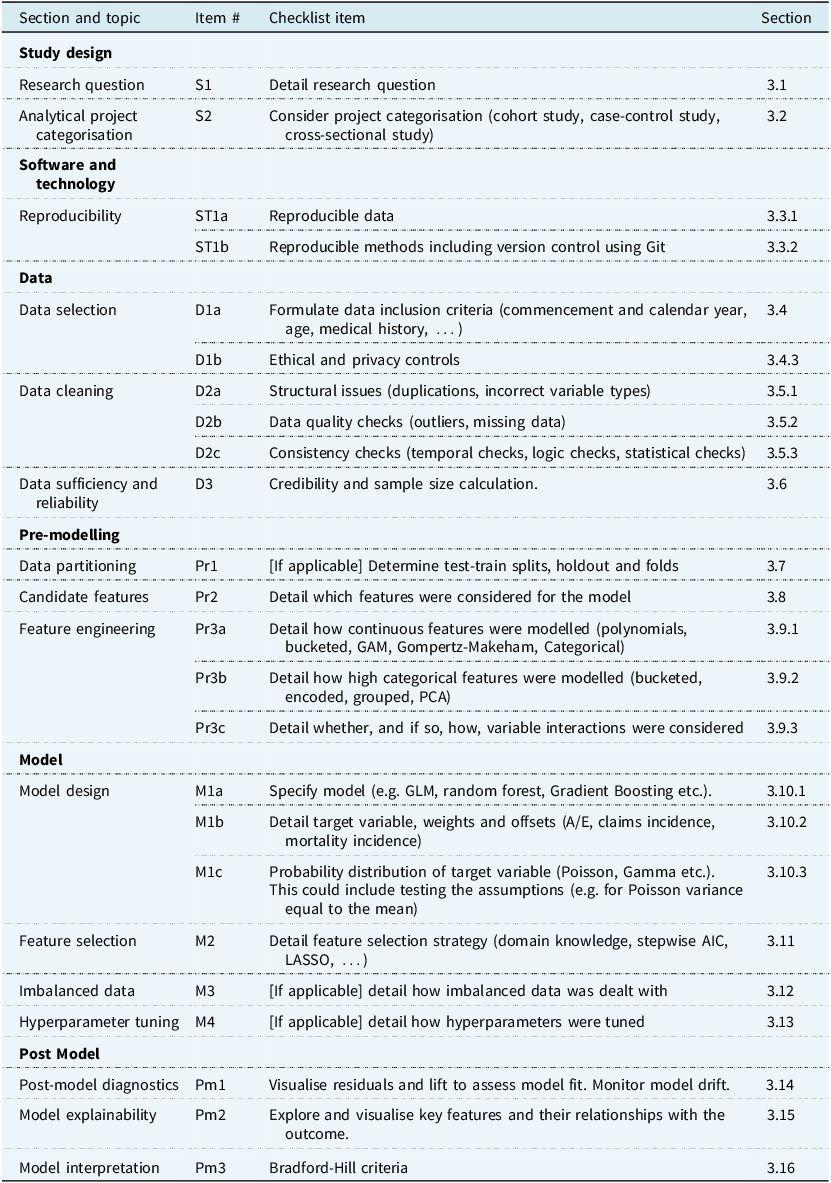
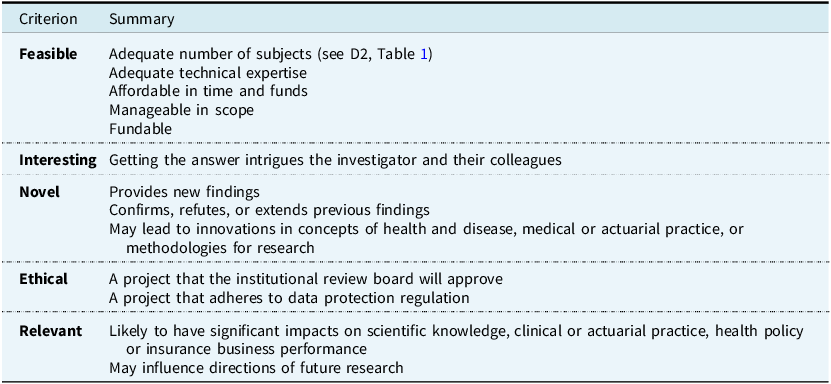
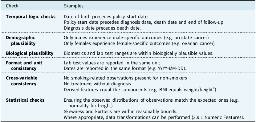
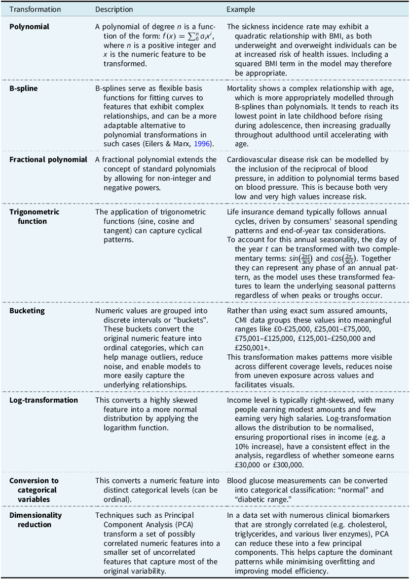
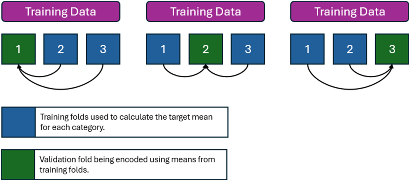

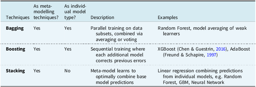


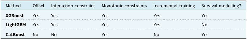


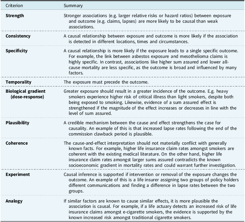

 Open access