


1 Introduction
In this paper we study a diagrammatic approach to the theory of quantum symmetric pairs, using the string diagram calculus of monoidal categories and module categories over them. Such diagrammatic methods have proven to be extremely valuable in representation theory, especially via their role in the categorification of quantum groups and connections to link invariants. However, the use of these methods in the theory of quantum symmetric pairs has only just begun; see [Reference Bao, Shan, Wang and WebsterBSWW18, Reference Brundan, Wang and WebsterBWW23, Reference Brundan, Wang and WebsterBWW25].
Associated to a Lie algebra
 $\mathfrak {g}$
and an involutive Lie algebra automorphism
$\mathfrak {g}$
and an involutive Lie algebra automorphism
 $\theta \colon \mathfrak {g} \to \mathfrak {g}$
, one has the symmetric pair
$\theta \colon \mathfrak {g} \to \mathfrak {g}$
, one has the symmetric pair
 $(\mathfrak {g},\mathfrak {g}^\theta )$
. The universal enveloping algebra
$(\mathfrak {g},\mathfrak {g}^\theta )$
. The universal enveloping algebra
 $U(\mathfrak {g}^\theta )$
is a Hopf subalgebra of
$U(\mathfrak {g}^\theta )$
is a Hopf subalgebra of
 $U(\mathfrak {g})$
. Thus,
$U(\mathfrak {g})$
. Thus,
 $U(\mathfrak {g}^\theta )\text {-mod}$
is a monoidal category and the restriction functor
$U(\mathfrak {g}^\theta )\text {-mod}$
is a monoidal category and the restriction functor
 $U(\mathfrak {g})\text {-mod} \to U(\mathfrak {g}^\theta )\text {-mod}$
is monoidal. Moving to the setting of quantum enveloping algebras, the situation becomes more subtle since the quantum enveloping algebra
$U(\mathfrak {g})\text {-mod} \to U(\mathfrak {g}^\theta )\text {-mod}$
is monoidal. Moving to the setting of quantum enveloping algebras, the situation becomes more subtle since the quantum enveloping algebra
 $U_q(\mathfrak {g}^\theta )$
is not naturally a Hopf subalgebra of
$U_q(\mathfrak {g}^\theta )$
is not naturally a Hopf subalgebra of
 $U_q(\mathfrak {g})$
. A general theory of quantum symmetric pairs was developed for all finite types by Letzter in [Reference LetzterLet99] and then extended to the Kac–Moody setting by Kolb in [Reference KolbKol14]. In the quantum world,
$U_q(\mathfrak {g})$
. A general theory of quantum symmetric pairs was developed for all finite types by Letzter in [Reference LetzterLet99] and then extended to the Kac–Moody setting by Kolb in [Reference KolbKol14]. In the quantum world,
 $U(\mathfrak {g}^\theta )$
is replaced by a right coideal subalgebra of
$U(\mathfrak {g}^\theta )$
is replaced by a right coideal subalgebra of
 $U_q(\mathfrak {g})$
denoted by
$U_q(\mathfrak {g})$
denoted by
 $\mathrm {U}^\imath $
. In recent works extending this theory to the super setting and developing canonical basis theory,
$\mathrm {U}^\imath $
. In recent works extending this theory to the super setting and developing canonical basis theory,
 $\mathrm {U}^\imath $
is often referred to as an iquantum enveloping algebra. The category
$\mathrm {U}^\imath $
is often referred to as an iquantum enveloping algebra. The category
 $\mathrm {U}^\imath \text {-mod}$
is not a monoidal category, but it is a right module category over the monoidal category
$\mathrm {U}^\imath \text {-mod}$
is not a monoidal category, but it is a right module category over the monoidal category
 $U_q(\mathfrak {g})$
. The iquantum enveloping algebras and their representation theory have attracted increasing interest in recent years. It is becoming apparent that much of the theory of quantum enveloping algebras has natural analogues in the iquantum setting. We refer the reader to the exposition [Reference WangWan23] for an overview of this development. In particular, the theory of quantum symmetric pairs has been extended to the case of Lie superalgebras in [Reference Kolb and YakimovKY20, Reference ShenShe25, Reference Shen and WangSW25].
$U_q(\mathfrak {g})$
. The iquantum enveloping algebras and their representation theory have attracted increasing interest in recent years. It is becoming apparent that much of the theory of quantum enveloping algebras has natural analogues in the iquantum setting. We refer the reader to the exposition [Reference WangWan23] for an overview of this development. In particular, the theory of quantum symmetric pairs has been extended to the case of Lie superalgebras in [Reference Kolb and YakimovKY20, Reference ShenShe25, Reference Shen and WangSW25].
In the current paper, we focus on the case where
 $\mathfrak {g} = \mathfrak {gl}(m|2n)$
is the general linear Lie superalgebra and
$\mathfrak {g} = \mathfrak {gl}(m|2n)$
is the general linear Lie superalgebra and
 $\mathfrak {g}^\theta = \mathfrak {osp}(m|2n)$
is the orthosymplectic Lie superalgebra. Many features of the representation theory of
$\mathfrak {g}^\theta = \mathfrak {osp}(m|2n)$
is the orthosymplectic Lie superalgebra. Many features of the representation theory of
 $\mathrm {U} = U_q(\mathfrak {g})$
are captured in the framed HOMFLYPT skein category, or oriented skein category for short, denoted by
$\mathrm {U} = U_q(\mathfrak {g})$
are captured in the framed HOMFLYPT skein category, or oriented skein category for short, denoted by ![]() . This diagrammatic monoidal category, first introduced in [Reference TuraevTur89, §5.2], is a quotient of the category of framed oriented tangles and underpins the HOMFLYPT link invariant. The connection to representation theory arises from the fact that there is a full monoidal functor
. This diagrammatic monoidal category, first introduced in [Reference TuraevTur89, §5.2], is a quotient of the category of framed oriented tangles and underpins the HOMFLYPT link invariant. The connection to representation theory arises from the fact that there is a full monoidal functor
The analogous diagrammatic category for
 $U_q(\mathfrak {osp}(m|2n))$
is the Kauffman category, first introduced in [Reference TuraevTur89, §7.7]. However, since the usual quantum enveloping algebra
$U_q(\mathfrak {osp}(m|2n))$
is the Kauffman category, first introduced in [Reference TuraevTur89, §7.7]. However, since the usual quantum enveloping algebra
 $U_q(\mathfrak {osp}(m|2n))$
is not the correct starting point for quantizing the symmetric pair
$U_q(\mathfrak {osp}(m|2n))$
is not the correct starting point for quantizing the symmetric pair
 $(\mathfrak {g},\mathfrak {g}^\theta )$
, the Kauffman category is not well suited for the diagrammatic study of the representation theory of
$(\mathfrak {g},\mathfrak {g}^\theta )$
, the Kauffman category is not well suited for the diagrammatic study of the representation theory of
 $\mathrm {U}^\imath \text {-mod}$
.
$\mathrm {U}^\imath \text {-mod}$
.
Because
 $\mathrm {U}^\imath \text {-mod}$
is a right module category over
$\mathrm {U}^\imath \text {-mod}$
is a right module category over
 $\mathrm {U}\text {-mod}$
, it is natural to expect that a diagrammatic description of
$\mathrm {U}\text {-mod}$
, it is natural to expect that a diagrammatic description of
 $\mathrm {U}^\imath \text {-mod}$
should be given by a right module category over
$\mathrm {U}^\imath \text {-mod}$
should be given by a right module category over ![]() . We restrict our attention to the category
. We restrict our attention to the category
 $\mathrm {U}\text {-tmod}$
of tensor modules. By definition, this is the full subcategory of
$\mathrm {U}\text {-tmod}$
of tensor modules. By definition, this is the full subcategory of
 $\mathrm {U}$
-modules whose objects are finite direct summands of tensor products of the natural module
$\mathrm {U}$
-modules whose objects are finite direct summands of tensor products of the natural module
 $V^+$
and its dual
$V^+$
and its dual
 $V^-$
. A key observation is that the natural module and its dual become isomorphic after restriction to
$V^-$
. A key observation is that the natural module and its dual become isomorphic after restriction to
 $\mathrm {U}^\imath $
. Thus, there is an isomorphism (Lemma 5.6)
$\mathrm {U}^\imath $
. Thus, there is an isomorphism (Lemma 5.6)
 $$\begin{align*}\varphi \colon V^- \xrightarrow{\cong} V^+ \qquad \text{of } \mathrm{U}^\imath\text{-modules}. \end{align*}$$
It turns out that, in a way that we make precise in the current paper, this isomorphism determines the module category structure of
 $\mathrm {U}^\imath \text {-tmod}$
over
$\mathrm {U}^\imath \text {-tmod}$
over
 $\mathrm {U}\text {-tmod}$
.
$\mathrm {U}\text {-tmod}$
.
The oriented skein category ![]() is generated by two objects,
is generated by two objects,
 ${\mathord {\uparrow }}$
and
${\mathord {\uparrow }}$
and
 ${\mathord {\downarrow }}$
, which are the diagrammatic analogues of the natural module and its dual. We define the disoriented skein category,
${\mathord {\downarrow }}$
, which are the diagrammatic analogues of the natural module and its dual. We define the disoriented skein category, ![]() , to be the right module category over
, to be the right module category over ![]() generated by mutually inverse isomorphisms
generated by mutually inverse isomorphisms
subject to relations that can be found in (2.17) and (2.18). Then, in Section 2.2, we define a morphism of module categories
We prove (Theorem 8.1) that the functor ![]() is full.
is full.
There is another diagrammatic category that has appeared in the literature in connection to the representation theory of
 $\mathrm {U}^\imath $
. This category was based on the q-Brauer algebras used in [Reference MolevMol03, Reference WenzlWen12] to study the endomorphism algebras
$\mathrm {U}^\imath $
. This category was based on the q-Brauer algebras used in [Reference MolevMol03, Reference WenzlWen12] to study the endomorphism algebras
 $\operatorname {\mathrm {End}}_{\mathrm {U}^\imath }((V^+)^{\otimes r})$
. These algebras were incorporated into a q-Brauer category
$\operatorname {\mathrm {End}}_{\mathrm {U}^\imath }((V^+)^{\otimes r})$
. These algebras were incorporated into a q-Brauer category ![]() in [Reference Sartori and TubbenhauerST19], and there is a full functor (Theorem 8.1)
in [Reference Sartori and TubbenhauerST19], and there is a full functor (Theorem 8.1)
In this paper we will use the term iquantum Brauer instead of q-Brauer; see Remark 7.4. The category ![]() was defined in [Reference Sartori and TubbenhauerST19, Def. 7.9] as a module category over a monoidal category version of the tower of Iwahori–Hecke algebras of type A. Given its connection to representation theory, it is natural to expect that
was defined in [Reference Sartori and TubbenhauerST19, Def. 7.9] as a module category over a monoidal category version of the tower of Iwahori–Hecke algebras of type A. Given its connection to representation theory, it is natural to expect that ![]() is also a right module category over
is also a right module category over ![]() . In fact, the search for this structure was the original motivation for the current paper. We describe this module category structure explicitly in Section 3.
. In fact, the search for this structure was the original motivation for the current paper. We describe this module category structure explicitly in Section 3.
We show in Theorem 4.5 that the categories ![]() and
and ![]() are equivalent as right module categories over
are equivalent as right module categories over ![]() . This equivalence is compatible with the functors to the categories of
. This equivalence is compatible with the functors to the categories of
 $\mathrm {U}^\imath $
-modules. Setting
$\mathrm {U}^\imath $
-modules. Setting ![]() ,
, ![]() , and
, and ![]() , our main results can be summarized in the following diagram:
, our main results can be summarized in the following diagram:

The horizontal arrows labelled
 $\otimes $
are the right module category structures, while the functors
$\otimes $
are the right module category structures, while the functors
 $\mathbf {F}$
and
$\mathbf {F}$
and
 $\mathbf {G}$
give the equivalence of module categories between
$\mathbf {G}$
give the equivalence of module categories between ![]() and
and ![]() . The diagram (1.1) illustrates an important advantage of the disoriented skein category over the iquantum Brauer category: the top square in (1.1) commutes, while the bottom square only commutes up to natural isomorphism. This corresponds to the fact that
. The diagram (1.1) illustrates an important advantage of the disoriented skein category over the iquantum Brauer category: the top square in (1.1) commutes, while the bottom square only commutes up to natural isomorphism. This corresponds to the fact that ![]() is a strict morphism of
is a strict morphism of ![]() -modules, whereas
-modules, whereas ![]() is a morphism of
is a morphism of ![]() -modules that is not strict. The
-modules that is not strict. The ![]() -module structure is also simpler for
-module structure is also simpler for ![]() than it is for
than it is for ![]() . Yet another benefit of
. Yet another benefit of ![]() is that the diagrams can contain cups and caps in arbitrary positions, whereas the cups and caps in
is that the diagrams can contain cups and caps in arbitrary positions, whereas the cups and caps in ![]() can only appear on the left side of diagrams. The resulting duality in
can only appear on the left side of diagrams. The resulting duality in ![]() makes it much easier to prove a basis theorem describing bases for the morphism spaces (Theorem 7.1). Using the equivalences
makes it much easier to prove a basis theorem describing bases for the morphism spaces (Theorem 7.1). Using the equivalences
 $\mathbf {F}$
and
$\mathbf {F}$
and
 $\mathbf {G}$
, one can then deduce a basis theorem for
$\mathbf {G}$
, one can then deduce a basis theorem for ![]() (Corollary 7.2).
(Corollary 7.2).
The categories ![]() and
and ![]() should both be thought of as interpolating categories for the categories of
should both be thought of as interpolating categories for the categories of
 $\mathrm {U}^\imath $
-modules, similar to the interpolating categories introduced by Deligne [Reference DeligneDel07]. The benefits of the disoriented skein category
$\mathrm {U}^\imath $
-modules, similar to the interpolating categories introduced by Deligne [Reference DeligneDel07]. The benefits of the disoriented skein category ![]() over the iquantum Brauer category
over the iquantum Brauer category ![]() arise from the fact that the former category contains generating objects corresponding to the restriction to
arise from the fact that the former category contains generating objects corresponding to the restriction to
 $\mathrm {U}^\imath $
of the natural
$\mathrm {U}^\imath $
of the natural
 $\mathrm {U}$
-module
$\mathrm {U}$
-module
 $V^+$
and its dual
$V^+$
and its dual
 $V^-$
, whereas the latter category only contains a generating object corresponding to
$V^-$
, whereas the latter category only contains a generating object corresponding to
 $V^+$
. Even though
$V^+$
. Even though
 $V^+$
and
$V^+$
and
 $V^-$
are isomorphic as
$V^-$
are isomorphic as
 $\mathrm {U}^\imath $
-modules, including them both in the diagrammatics allows greater flexibility and better compatibility with the structure of a module category over
$\mathrm {U}^\imath $
-modules, including them both in the diagrammatics allows greater flexibility and better compatibility with the structure of a module category over
 $\mathrm {U}\text {-tmod}$
, where
$\mathrm {U}\text {-tmod}$
, where
 $V^+$
and
$V^+$
and
 $V^-$
are not isomorphic.
$V^-$
are not isomorphic.
We conclude this introduction with some possible directions for future research. The most obvious open question is to describe the kernel of the functors ![]() and
and ![]() . Since these functors are full, a precise description of the kernel would give a complete presentation of the categories of tensor modules. We hope to explore this in upcoming work.
. Since these functors are full, a precise description of the kernel would give a complete presentation of the categories of tensor modules. We hope to explore this in upcoming work.
We expect that the methods developed in the current paper can be used to develop diagrammatics for other quantum symmetric pairs. For any quantum symmetric pair
 $(\mathrm {U},\mathrm {U}^\imath )$
for which there exists a good diagrammatic calculus for the representation theory of
$(\mathrm {U},\mathrm {U}^\imath )$
for which there exists a good diagrammatic calculus for the representation theory of
 $\mathrm {U}$
, one should be able to develop a diagrammatics calculus for the representation theory of
$\mathrm {U}$
, one should be able to develop a diagrammatics calculus for the representation theory of
 $\mathrm {U}^\imath $
in a matter analogous to the definition of
$\mathrm {U}^\imath $
in a matter analogous to the definition of ![]() from
from ![]() .
.
Recently, the Brauer and Kauffman categories have been extended in [Reference McNamara and SavageMS24, Reference McNamara and SavageMS25] to incorporate the spin representation. However, the iquantum Brauer category only captures the behaviour of tensor modules for
 $\mathrm {U}^\imath $
, which are all obtained by restriction from
$\mathrm {U}^\imath $
, which are all obtained by restriction from
 $\mathrm {U}$
-modules. It would be interesting to enlarge
$\mathrm {U}$
-modules. It would be interesting to enlarge ![]() to a module category over
to a module category over ![]() that incorporates a larger class of modules. In particular, there should be an iquantum analogue of the quantum spin Brauer category of [Reference McNamara and SavageMS25]. There should also be affine and cyclotomic analogues of both the disoriented skein and iquantum Brauer categories, analogous to the affine and cyclotomic versions of the oriented Brauer, oriented skein, Brauer, and Kauffman categories studied in [Reference Brundan, Comes, Nash and ReynoldsBCNR17, Reference BrundanBru17, Reference Rui and SongRS19, Reference Gao, Rui and SongGRS22, Reference Savage and WebsterSW].
that incorporates a larger class of modules. In particular, there should be an iquantum analogue of the quantum spin Brauer category of [Reference McNamara and SavageMS25]. There should also be affine and cyclotomic analogues of both the disoriented skein and iquantum Brauer categories, analogous to the affine and cyclotomic versions of the oriented Brauer, oriented skein, Brauer, and Kauffman categories studied in [Reference Brundan, Comes, Nash and ReynoldsBCNR17, Reference BrundanBru17, Reference Rui and SongRS19, Reference Gao, Rui and SongGRS22, Reference Savage and WebsterSW].
Another diagrammatic approach to representation theory involves the theory of webs. In [Reference Sartori and TubbenhauerST19], the authors introduce categories that should be viewed as web versions of the iquantum Brauer category. One should also be able to define a web version of the disoriented skein category by taking a partial idempotent completion at idempotents corresponding to quantum symmetrizers and antisymmetrizers. This disoriented web category should be a module category over the web categories of [Reference Cautis, Kamnitzer and MorrisonCKM14]. We expect that the relationship between this disoriented web category and the web categories of [Reference Sartori and TubbenhauerST19] would be analogous to the relationship between the disoriented skein category and the iquantum Brauer category.
2 Diagrammatic categories
In this section we introduce the diagrammatic categories of interest to us. Throughout this section
 $\Bbbk $
is an arbitrary commutative ring and
$\Bbbk $
is an arbitrary commutative ring and
 $q,t$
are elements of
$q,t$
are elements of
 $\Bbbk ^\times $
such that
$\Bbbk ^\times $
such that
 $t-t^{-1}$
is divisible by
$t-t^{-1}$
is divisible by
 $q-q^{-1}$
. We assume that we have a ring automorphism
$q-q^{-1}$
. We assume that we have a ring automorphism
 $\xi $
of
$\xi $
of
 $\Bbbk $
such that
$\Bbbk $
such that
 $\xi (q) = q^{-1}$
and
$\xi (q) = q^{-1}$
and
 $\xi (t)=t^{-1}$
. If
$\xi (t)=t^{-1}$
. If
 $\mathcal {C}$
and
$\mathcal {C}$
and
 $\mathcal {D}$
are
$\mathcal {D}$
are
 $\Bbbk $
-linear categories, we say that a functor
$\Bbbk $
-linear categories, we say that a functor
 $\mathbf {H} \colon \mathcal {C} \to \mathcal {D}$
is
$\mathbf {H} \colon \mathcal {C} \to \mathcal {D}$
is
 $\Bbbk $
-antilinear if
$\Bbbk $
-antilinear if
 $\mathbf {H}(a f + b g) = \xi (a) \mathbf {H}(f) + \xi (b) \mathbf {H}(g)$
for all morphisms f and g in the same morphism space of
$\mathbf {H}(a f + b g) = \xi (a) \mathbf {H}(f) + \xi (b) \mathbf {H}(g)$
for all morphisms f and g in the same morphism space of
 $\mathcal {C}$
.
$\mathcal {C}$
.
2.1 The oriented skein category
The framed HOMFLYPT skein category, or oriented skein category for short, ![]() , is the
, is the
 $\Bbbk $
-linear strict monoidal category generated by objects
$\Bbbk $
-linear strict monoidal category generated by objects
 ${\mathord {\uparrow }}$
,
${\mathord {\uparrow }}$
,
 ${\mathord {\downarrow }}$
and morphisms
${\mathord {\downarrow }}$
and morphisms
subject to the relations


In (2.1), we have used the following morphisms:
This category was first introduced in [Reference TuraevTur89, §5.2], where it was called the Hecke category. In [Reference Queffelec and SartoriQS19, Definition 2.1] it is called the quantized oriented Brauer category. It was studied in depth in [Reference BrundanBru17]. Note that in [Reference BrundanBru17], the category is denoted ![]() , with the denominator
, with the denominator
 $q-q^{-1}$
in (2.3) replaced by z. Since we will only be interested in the case
$q-q^{-1}$
in (2.3) replaced by z. Since we will only be interested in the case
 $z=q-q^{-1}$
, we make this choice at the start and use the simpler notation
$z=q-q^{-1}$
, we make this choice at the start and use the simpler notation ![]() instead of
instead of ![]() .
.
We define the following morphisms:
The category ![]() is strict pivotal. Furthermore, the following relations hold for any orientation of the strands:
is strict pivotal. Furthermore, the following relations hold for any orientation of the strands:

We also have
It is straightforward to verify that there is a
 $\Bbbk $
-antilinear isomorphism of monoidal categories
$\Bbbk $
-antilinear isomorphism of monoidal categories
acting on objects as
 ${\mathord {\uparrow }} \mapsto {\mathord {\downarrow }}$
,
${\mathord {\uparrow }} \mapsto {\mathord {\downarrow }}$
,
 ${\mathord {\downarrow }} \mapsto {\mathord {\uparrow }}$
, and sending
${\mathord {\downarrow }} \mapsto {\mathord {\uparrow }}$
, and sending
Intuitively,
 $\Omega _{\updownarrow }$
reflects diagrams in the horizontal axis and inverts q and t. We also have an isomorphism of
$\Omega _{\updownarrow }$
reflects diagrams in the horizontal axis and inverts q and t. We also have an isomorphism of
 $\Bbbk $
-linear monoidal categories
$\Bbbk $
-linear monoidal categories
that reverses the orientation of all strands. Finally, we have a
 $\Bbbk $
-antilinear isomorphism of monoidal categories
$\Bbbk $
-antilinear isomorphism of monoidal categories
which we call the bar involution, acting as the identity on objects and given on morphisms by
Intuitively, the bar involution flips crossings in diagrams and inverts q and t.
Let
 $\langle {\mathord {\uparrow }},{\mathord {\downarrow }} \rangle $
denote the set of objects for
$\langle {\mathord {\uparrow }},{\mathord {\downarrow }} \rangle $
denote the set of objects for ![]() . Equivalently, writing the tensor product as juxtaposition,
. Equivalently, writing the tensor product as juxtaposition,
 $\langle {\mathord {\uparrow }},{\mathord {\downarrow }} \rangle $
is the set of words generated by
$\langle {\mathord {\uparrow }},{\mathord {\downarrow }} \rangle $
is the set of words generated by
 ${\mathord {\uparrow }}$
and
${\mathord {\uparrow }}$
and
 ${\mathord {\downarrow }}$
. It will be convenient to introduce thick strands:
${\mathord {\downarrow }}$
. It will be convenient to introduce thick strands:

The fact that ![]() is a braided monoidal category gives us a natural interpretation for crossings of such strands. For instance, if
is a braided monoidal category gives us a natural interpretation for crossings of such strands. For instance, if
 $\lambda = {\mathord {\downarrow }} {\mathord {\uparrow }}$
and
$\lambda = {\mathord {\downarrow }} {\mathord {\uparrow }}$
and
 $\mu = {\mathord {\uparrow }} {\mathord {\uparrow }} {\mathord {\downarrow }}$
, then
$\mu = {\mathord {\uparrow }} {\mathord {\uparrow }} {\mathord {\downarrow }}$
, then

2.2 The disoriented skein category
Let ![]() be a
be a
 $\Bbbk $
-linear strict monoidal category, and let
$\Bbbk $
-linear strict monoidal category, and let
 $\mathcal {M}$
be a
$\mathcal {M}$
be a
 $\Bbbk $
-linear category. Let
$\Bbbk $
-linear category. Let ![]() denote the strict monoidal category of
denote the strict monoidal category of
 $\Bbbk $
-linear endofunctors of
$\Bbbk $
-linear endofunctors of
 $\mathcal {M}$
. A right action of
$\mathcal {M}$
. A right action of
 $\mathcal {C}$
on
$\mathcal {C}$
on
 $\mathcal {M}$
is a monoidal functor
$\mathcal {M}$
is a monoidal functor ![]() , where
, where
 $\mathcal {D}^{\text {rev}}$
denotes the reverse of a monoidal category
$\mathcal {D}^{\text {rev}}$
denotes the reverse of a monoidal category
 $\mathcal {D}$
, where we reverse the tensor product. Given such a right action, we also say that
$\mathcal {D}$
, where we reverse the tensor product. Given such a right action, we also say that
 $\mathcal {M}$
is a right module category over
$\mathcal {M}$
is a right module category over
 $\mathcal {C}$
, or
$\mathcal {C}$
, or
 $\mathcal {C}$
-module for short; see [Reference Etingof, Gelaki, Nikshych and OstrikEGNO15, §7.1]. For objects
$\mathcal {C}$
-module for short; see [Reference Etingof, Gelaki, Nikshych and OstrikEGNO15, §7.1]. For objects
 $C \in \mathcal {C}$
and
$C \in \mathcal {C}$
and
 $M \in \mathcal {M}$
, we set
$M \in \mathcal {M}$
, we set
 $$ \begin{align} M \otimes C := \mathbf{A}(C)(M). \end{align} $$
We say that the
 $\mathcal {C}$
-module
$\mathcal {C}$
-module
 $\mathcal {M}$
is strict if
$\mathcal {M}$
is strict if
 $\mathbf {A}$
is a strict monoidal functor. Equivalently,
$\mathbf {A}$
is a strict monoidal functor. Equivalently,
 $\mathcal {M}$
is strict if
$\mathcal {M}$
is strict if
 $$\begin{align*}M \otimes (C_1 \otimes C_2) = (M \otimes C_1) \otimes C_2,\qquad \text{for all } M \in \mathcal{M},\ C_1,C_2 \in \mathcal{C}, \end{align*}$$
and similarly for morphisms.
We now describe the notion of a presentation of
 $\mathcal {C}$
-modules by generators and relations. We restrict ourselves to the case where there are only generating morphisms (i.e., no nontrivial generating objects). Let
$\mathcal {C}$
-modules by generators and relations. We restrict ourselves to the case where there are only generating morphisms (i.e., no nontrivial generating objects). Let
 $\mathtt {M}$
be the set of generating morphisms. These are formal morphisms whose domains and codomains are objects of
$\mathtt {M}$
be the set of generating morphisms. These are formal morphisms whose domains and codomains are objects of
 $\mathcal {C}$
. Let
$\mathcal {C}$
. Let
 $\mathcal {M}$
be the
$\mathcal {M}$
be the
 $\Bbbk $
-linear category whose objects are the objects of
$\Bbbk $
-linear category whose objects are the objects of
 $\mathcal {C}$
and whose morphisms are generated (as a
$\mathcal {C}$
and whose morphisms are generated (as a
 $\Bbbk $
-linear category) by morphisms of
$\Bbbk $
-linear category) by morphisms of
 $\mathcal {C}$
and morphisms
$\mathcal {C}$
and morphisms
 $$\begin{align*}f \otimes g \colon \operatorname{\mathrm{dom}}(f) \otimes \operatorname{\mathrm{dom}}(g) \to \operatorname{\mathrm{codom}}(f) \otimes \operatorname{\mathrm{codom}}(g),\qquad f \in \mathtt{M},\ g \in \operatorname{\mathrm{Mor}}(\mathcal{C}), \end{align*}$$
modulo the relations
 $$ \begin{align} (1_Y \otimes g) \circ (f \otimes h) = f \otimes (g \circ h) = (f \otimes g) \circ (1_X \otimes h), \end{align} $$
for all
 $f \colon X \to Y$
in
$f \colon X \to Y$
in
 $\mathtt {M}$
and all composable morphisms
$\mathtt {M}$
and all composable morphisms
 $g,h$
in
$g,h$
in
 $\mathcal {C}$
. The category
$\mathcal {C}$
. The category
 $\mathcal {M}$
has a natural structure of a strict
$\mathcal {M}$
has a natural structure of a strict
 $\mathcal {C}$
-module. Now, let
$\mathcal {C}$
-module. Now, let
 $\mathtt {R}$
be a set of relations on the morphisms in
$\mathtt {R}$
be a set of relations on the morphisms in
 $\mathcal {M}$
. Define
$\mathcal {M}$
. Define
 $\hat {\mathtt {R}}$
to be the smallest subset of morphisms of
$\hat {\mathtt {R}}$
to be the smallest subset of morphisms of
 $\mathcal {M}$
containing
$\mathcal {M}$
containing
 $\mathtt {R}$
and closed under composition, acting on the right by morphisms in
$\mathtt {R}$
and closed under composition, acting on the right by morphisms in
 $\mathcal {C}$
, and taking
$\mathcal {C}$
, and taking
 $\Bbbk $
-linear combinations. Then we define the
$\Bbbk $
-linear combinations. Then we define the
 $\mathcal {C}$
-module generated by the morphisms
$\mathcal {C}$
-module generated by the morphisms
 $\mathtt {M}$
subject to the relations
$\mathtt {M}$
subject to the relations
 $\mathtt {R}$
to be the quotient of
$\mathtt {R}$
to be the quotient of
 $\mathcal {M}$
by
$\mathcal {M}$
by
 $\hat {\mathtt {R}}$
. This has the structure of a strict
$\hat {\mathtt {R}}$
. This has the structure of a strict
 $\mathcal {C}$
-module induced from the
$\mathcal {C}$
-module induced from the
 $\mathcal {C}$
-module structure on
$\mathcal {C}$
-module structure on
 $\mathcal {M}$
.
$\mathcal {M}$
.
Using the usual string diagram notation for module categories, the relations (2.15) become

Definition 2.1. The disoriented skein category ![]() is the
is the ![]() -module generated by the morphisms
-module generated by the morphisms
which we call toggles, subject to the relations

Lemma 2.2. The following relations hold in ![]() :
:
Proof. Composing on the top of the last relation in (2.17) with ![]() , then using the first relation in (2.17) gives
, then using the first relation in (2.17) gives

Multiplying both sides by t then yields the first relation in (2.19). The proof of the second relation in (2.19) is similar.
The next lemma shows that the relations (2.17) to (2.19) hold after flipping crossings and inverting q.
Lemma 2.3. The following relations hold in ![]() :
:

Proof. The first relation in (2.20) follows from the first relation in (2.18) after composing on the bottom with ![]() and using (2.1). The proofs of the second, third, and fourth relations in (2.20) are analogous.
and using (2.1). The proofs of the second, third, and fourth relations in (2.20) are analogous.
Let
 $z=q-q^{-1}$
. We have
$z=q-q^{-1}$
. We have

and

Subtracting and using the third relation in (2.17) then yields (2.21).
We note that a diagram representing a morphism in ![]() can only have
can only have ![]() or
or ![]() appearing on the leftmost strand. However, we define the following morphisms:
appearing on the leftmost strand. However, we define the following morphisms:

Using (2.22) and the module category structure of ![]() , we may now draw diagrams with
, we may now draw diagrams with ![]() and
and ![]() appearing on any strand and interpret them as morphisms in
appearing on any strand and interpret them as morphisms in ![]() .
.
Lemma 2.4. The following relations hold in ![]() for any
for any
 $\lambda ,\mu \in \langle {\mathord {\uparrow }},{\mathord {\downarrow }} \rangle $
:
$\lambda ,\mu \in \langle {\mathord {\uparrow }},{\mathord {\downarrow }} \rangle $
:


Proof. The equalities (2.23) and (2.25) follow easily from (2.17) and (2.22). To prove the first relation in (2.24), it suffices to prove that

where, in the braces, the strands in the cups and caps can have any orientation, and
 $\lambda ,\mu $
run over all objects of
$\lambda ,\mu $
run over all objects of ![]() . For
. For  , we have

Composing on the top and bottom with

respectively, then using (2.17), yields the case  . The remaining cases for f follow easily from (2.7), (2.8) and (2.16). This completes the proof of the first relation in (2.24). The proof of the second relation then follows by composing the first relation on the top and bottom with

respectively, then using (2.17).
To prove the first equality in (2.26), we have

The remaining relations in (2.26) are proved similarly. Note also that one can apply
 $\Omega _\updownarrow $
, defined in (2.27) below, to obtain the second and fourth equalities from the first and third, respectively.
$\Omega _\updownarrow $
, defined in (2.27) below, to obtain the second and fourth equalities from the first and third, respectively.
In light of (2.24), we define toggles at the same height by
and similarly for the other toggles, or for more than two toggles at the same height.
Remark 2.5. We emphasize that ![]() is not a monoidal category. For example, the relations in (2.18) and (2.26) do not hold, in general, unless they are on the left side of a diagram. For instance, since
is not a monoidal category. For example, the relations in (2.18) and (2.26) do not hold, in general, unless they are on the left side of a diagram. For instance, since

we cannot apply the last relation in (2.18) to the curl with a toggle directly in this situation.
We now describe three natural symmetries of the disoriented skein category. First, it follows from Lemma 2.3 that the isomorphism (2.10) induces a
 $\Bbbk $
-antilinear isomorphism of categories
$\Bbbk $
-antilinear isomorphism of categories
such that the diagram

commutes.
Second, (2.12) induces an isomorphism of
 $\Bbbk $
-linear categories
$\Bbbk $
-linear categories
such that the following diagram commutes:

Indeed,
 $\Theta $
respects the relations (2.18) by (2.19), and it respects the last relation in (2.17) by (2.22) and the
$\Theta $
respects the relations (2.18) by (2.19), and it respects the last relation in (2.17) by (2.22) and the ![]() case of the last relation in (2.24).
case of the last relation in (2.24).
Finally, it follows from Lemma 2.3 that the bar involution (2.13) induces a
 $\Bbbk $
-antilinear isomorphism of categories
$\Bbbk $
-antilinear isomorphism of categories
such that the following diagram commutes:

Note that,
 $\Omega _\updownarrow $
,
$\Omega _\updownarrow $
,
 $\Theta $
, and
$\Theta $
, and
 $\Xi $
do not behave well with respect to toggles on strands that are not on the left, due to the crossings in (2.22). However, the composites
$\Xi $
do not behave well with respect to toggles on strands that are not on the left, due to the crossings in (2.22). However, the composites
 $\Theta \circ \Xi $
and
$\Theta \circ \Xi $
and
 $\Omega _\updownarrow \circ \Theta $
do behave well: they act as
$\Omega _\updownarrow \circ \Theta $
do behave well: they act as ![]() ,
, ![]() on toggles in arbitrary position. Similarly,
on toggles in arbitrary position. Similarly,
 $\Omega _\updownarrow \circ \Xi $
acts as
$\Omega _\updownarrow \circ \Xi $
acts as ![]() ,
, ![]() on toggles in arbitrary position.
on toggles in arbitrary position.
Remark 2.6. The last relation in (2.17) is a twisted analogue of the reflection equation appearing in the definition of braided module categories; see Remark 6.5. In the corresponding categories of modules over quantum enveloping algebras and their coideal subalgebras, this twist is handled in [Reference KolbKol20] by passing to an equivariantization of the category of modules.
2.3 The iquantum Brauer category
We now recall the definition of the iquantum Brauer category. This category was defined in [Reference Sartori and TubbenhauerST19, Def. 7.9], where it was called the quantum or q-Brauer category. Its endomorphism algebras first appeared in [Reference MolevMol03, Def. 2.1]. The definition in [Reference Sartori and TubbenhauerST19, Def. 7.9] is as a module category over the subcategory of ![]() consisting of only upward-oriented strands. We start with a presentation as a
consisting of only upward-oriented strands. We start with a presentation as a
 $\Bbbk $
-linear category. Then, in Section 3, we endow the iquantum Brauer category with the structure of an
$\Bbbk $
-linear category. Then, in Section 3, we endow the iquantum Brauer category with the structure of an ![]() -module category, extending the module category structure from [Reference Sartori and TubbenhauerST19, Def. 7.9]. Below and throughout the paper, we let
-module category, extending the module category structure from [Reference Sartori and TubbenhauerST19, Def. 7.9]. Below and throughout the paper, we let
 $\mathbb {N}$
denote the set of nonnegative integers.
$\mathbb {N}$
denote the set of nonnegative integers.
Definition 2.7. The iquantum Brauer category ![]() is the
is the
 $\Bbbk $
-linear category with objects
$\Bbbk $
-linear category with objects
 $\mathsf {B}_r$
,
$\mathsf {B}_r$
,
 $r \in \mathbb {N}$
, and generating morphisms
$r \in \mathbb {N}$
, and generating morphisms
subject to relations that we describe below. We denote the identity morphism of
 $\mathsf {B}_r$
by the thick strand
$\mathsf {B}_r$
by the thick strand ![]() . We define juxtaposition of thick strands by
. We define juxtaposition of thick strands by
We use (2.32) even when these strands are part of a larger diagram that involves cups, caps, or crossings.
We impose the following relations on morphisms, for all
 $r,s \in \mathbb {N}$
:
$r,s \in \mathbb {N}$
:


where, in (2.37), f runs over all generating morphisms, g runs over the generating morphisms (2.31), and we interpret the juxtaposition using (2.32). For example, when
then (2.37) becomes

This concludes the definition of ![]() .
.
We define cups and caps appearing at the same height by

Note that

A similar argument (or, alternatively, composing the second and third relations in (2.35) with the appropriate crossings, then using the first two relations in (2.33)) gives

Note that the third relation in (2.36) is obtained from the second by reflecting the diagrams in the horizontal axis. The next result shows that the diagrammatic relation obtained by reflecting the first relation in (2.36) also holds.
Lemma 2.8. In ![]() ,
,

Proof. We have

Since

and

the result follows.
Lemma 2.9. There is a
 $\Bbbk $
-antilinear isomorphism of categories
$\Bbbk $
-antilinear isomorphism of categories
sending
Intuitively,
 $\Omega _\updownarrow $
reflects diagrams in a horizontal axis and inverts q and t.
$\Omega _\updownarrow $
reflects diagrams in a horizontal axis and inverts q and t.
Proof. Using (2.39) to (2.41), it is straightforward to verify that
 $\Omega _\updownarrow $
preserves the defining relations of
$\Omega _\updownarrow $
preserves the defining relations of ![]() . Since
. Since
 $\Omega _\updownarrow $
squares to the identity, it is an isomorphism.
$\Omega _\updownarrow $
squares to the identity, it is an isomorphism.
The following proposition implies that the relations (2.36) continue to hold after all crossings are flipped.
Proposition 2.10. In ![]() ,
,

Proof. The second and third relations in (2.43) follow from applying the isomorphism
 $\Omega _{\updownarrow }$
to the third and second relations, respectively, in (2.36). Thus, it remains to prove the first relation in (2.43).
$\Omega _{\updownarrow }$
to the third and second relations, respectively, in (2.36). Thus, it remains to prove the first relation in (2.43).
Let
 $z=q-q^{-1}$
. We repeatedly use the skein relation (2.34) to flip crossings:
$z=q-q^{-1}$
. We repeatedly use the skein relation (2.34) to flip crossings:


Adding together all the extra terms that appeared above gives z times

Thus, the first relation in (2.43) is satisfied.
Lemma 2.11. There is a
 $\Bbbk $
-antilinear isomorphism of categories
$\Bbbk $
-antilinear isomorphism of categories
which we call the bar involution, sending
Proof. Using (2.39), (2.40) and (2.43), it is straightforward to verify that the given map preserves the defining relations of ![]() . Since it squares to the identity, it is an isomorphism.
. Since it squares to the identity, it is an isomorphism.
Remark 2.12. In [Reference Cui and ShenCS24, Lem. 3.2], a bar involution was constructed for the iquantum Brauer algebras, which are isomorphic to endomorphism algebras of ![]() ; see Proposition 7.5. The bar involution in Lemma 2.11 is a generalization of this involution from the algebra level to the category level.
; see Proposition 7.5. The bar involution in Lemma 2.11 is a generalization of this involution from the algebra level to the category level.
Remark 2.13. For the reader familiar with the string diagram calculus for monoidal categories, we want to emphasize that the iquantum Brauer category is not monoidal. In particular, we may not, in general, use horizontal juxtaposition, which is the tensor product for monoidal categories. This is why we have been careful in (2.32) and (2.37) to define some particular horizontal juxtapositions; otherwise these would not be defined.
Remark 2.14. Taking
 $\Bbbk = \mathbb {Z}[q,q^{-1}]$
and
$\Bbbk = \mathbb {Z}[q,q^{-1}]$
and
 $t=q^m$
for some
$t=q^m$
for some
 $m \in \mathbb {Z}$
, the coefficient
$m \in \mathbb {Z}$
, the coefficient
 $(t-t^{-1})/(q-q^{-1})$
appearing in (2.35) becomes the quantum integer
$(t-t^{-1})/(q-q^{-1})$
appearing in (2.35) becomes the quantum integer
 $[m]$
; see (5.2). Then, specializing
$[m]$
; see (5.2). Then, specializing
 $q=1$
, the iquantum Brauer category becomes isomorphic to the usual Brauer category; see Corollary 7.3. Note, however, that the usual Brauer category is monoidal.
$q=1$
, the iquantum Brauer category becomes isomorphic to the usual Brauer category; see Corollary 7.3. Note, however, that the usual Brauer category is monoidal.
3 Module category structure on the iquantum Brauer category
The goal of the current section is to endow ![]() with the structure of a strict right module category over
with the structure of a strict right module category over ![]() . As noted in Section 2.2, this amounts to defining a strict monoidal functor
. As noted in Section 2.2, this amounts to defining a strict monoidal functor
We begin by defining functors that describe the action of the objects of ![]() . Recall the convention (2.32) for juxtaposition of strands in
. Recall the convention (2.32) for juxtaposition of strands in ![]() . We define the following thick crossings:
. We define the following thick crossings:

We then define
 $\Bbbk $
-linear endofunctors
$\Bbbk $
-linear endofunctors
 $\mathbf {A}_k$
,
$\mathbf {A}_k$
,
 $k \in \mathbb {N}$
, of
$k \in \mathbb {N}$
, of ![]() given on objects by
given on objects by
 $$ \begin{align} \mathbf{A}_k (\mathsf{B}_r) = \mathsf{B}_{r+k},\qquad r \in \mathbb{N}, \end{align} $$
and on morphisms by

for any morphism
 $f \colon \mathsf {B}_r \to \mathsf {B}_s$
in
$f \colon \mathsf {B}_r \to \mathsf {B}_s$
in ![]() . It is straightforward to verify that these define endofunctors of
. It is straightforward to verify that these define endofunctors of ![]() , for example, that they respect the defining relations of
, for example, that they respect the defining relations of ![]() .
.
Proposition 3.1. We have natural transformations
with components given as follows:

Proof. To show that ![]() is a natural transformation, we must show that, for
is a natural transformation, we must show that, for
 $r,s \in \mathbb {N}$
, and
$r,s \in \mathbb {N}$
, and
 $f \colon \mathsf {B}_r \to \mathsf {B}_s$
a morphism in
$f \colon \mathsf {B}_r \to \mathsf {B}_s$
a morphism in ![]() , the diagram
, the diagram

commutes. This follows immediately from (2.37). Hence ![]() is a natural transformation. The proof that
is a natural transformation. The proof that ![]() is a natural transformation is similar.
is a natural transformation is similar.
To show that ![]() is a natural transformation, we must show that, for f a generating morphism of
is a natural transformation, we must show that, for f a generating morphism of ![]() , the diagram
, the diagram

commutes. In other words, we must show that

When ![]() this is the third relation in (2.36). When
this is the third relation in (2.36). When ![]() it is (2.41). Finally, when
it is (2.41). Finally, when ![]() , (3.8) follows from (2.33) and (2.37). The proofs that
, (3.8) follows from (2.33) and (2.37). The proofs that ![]() ,
,
, and ![]() are natural transformations are analogous.
are natural transformations are analogous.
We will show in Theorem 3.3 that
 $\mathbf {A}$
yields a well-defined functor from
$\mathbf {A}$
yields a well-defined functor from ![]() . First, we extend
. First, we extend
 $\mathbf {A}$
to compositions and tensor products of generating morphisms by requiring that
$\mathbf {A}$
to compositions and tensor products of generating morphisms by requiring that
 $\mathbf {A}$
commute with these two operations. We will denote horizontal composition of natural transformations by
$\mathbf {A}$
commute with these two operations. We will denote horizontal composition of natural transformations by
 $*$
and the identity natural transformation of a functor
$*$
and the identity natural transformation of a functor
 $\mathbf {H}$
by
$\mathbf {H}$
by
 $\operatorname {\mathrm {id}}_{\mathbf {H}}$
.
$\operatorname {\mathrm {id}}_{\mathbf {H}}$
.
Lemma 3.2. For
 $n \in \mathbb {N}$
,
$n \in \mathbb {N}$
,

Proof. We first compute

Thus,

A similar computation shows that the second equality in (3.9) holds. Then we have

where the third equality above follows from the first equality in (3.9), and then the final equality above follows from our earlier computation of ![]() . The proof of the final equality in (3.9) is analogous, as are the relations (3.10).
. The proof of the final equality in (3.9) is analogous, as are the relations (3.10).
Theorem 3.3. We have a strict monoidal functor ![]() given on objects by
given on objects by
 ${\mathord {\uparrow }}, {\mathord {\downarrow }} \mapsto \mathbf {A}_1$
, and on morphisms by (3.3) and (3.4).
${\mathord {\uparrow }}, {\mathord {\downarrow }} \mapsto \mathbf {A}_1$
, and on morphisms by (3.3) and (3.4).
Proof. We must show that
 $\mathbf {A}$
respects the relations (2.1) to (2.4). The first three equalities in (2.1) follow immediately from (2.33). The last two equalities in (2.1) follow from (3.9). The fact that
$\mathbf {A}$
respects the relations (2.1) to (2.4). The first three equalities in (2.1) follow immediately from (2.33). The last two equalities in (2.1) follow from (3.9). The fact that
 $\mathbf {A}$
respects (2.2) follows from (2.34).
$\mathbf {A}$
respects (2.2) follows from (2.34).
For the first equality in (2.3), we compute

as desired. A similar computation shows that
 $\mathbf {A}$
respects the second equality in (2.3). For the third equality in (2.3), we have
$\mathbf {A}$
respects the second equality in (2.3). For the third equality in (2.3), we have

as desired.
For the first relation in (2.4), we compute

The proof that
 $\mathbf {A}$
respects the second relation in (2.4) is similar.
$\mathbf {A}$
respects the second relation in (2.4) is similar.
Written in module-theoretic (as opposed to representation-theoretic) notation, as in (2.14), the action defined in Theorem 3.3 is as follows. On objects,
 $$\begin{align*}\mathsf{B}_r \otimes {\mathord{\uparrow}} := \mathsf{B}_{r+1},\qquad \mathsf{B}_r \otimes {\mathord{\downarrow}} := \mathsf{B}_{r+1},\qquad r \in \mathbb{N}, \end{align*}$$
and, on morphisms,

for f a morphism in ![]() .
.
4 Equivalence of the disoriented skein and iquantum Brauer categories
In this section, we will show that the disoriented skein category ![]() and the iquantum Brauer category
and the iquantum Brauer category ![]() are equivalent as
are equivalent as ![]() -module categories.
-module categories.
4.1 Morphisms of module categories
Recall the definition of strict right module categories from Section 2.2. Let ![]() be a
be a
 $\Bbbk $
-linear strict monoidal category, and let
$\Bbbk $
-linear strict monoidal category, and let
 $\mathcal {M}$
,
$\mathcal {M}$
,
 $\mathcal {N}$
be strict
$\mathcal {N}$
be strict
 $\mathcal {C}$
-modules. A morphism of
$\mathcal {C}$
-modules. A morphism of
 $\mathcal {C}$
-modules from
$\mathcal {C}$
-modules from
 $\mathcal {M}$
to
$\mathcal {M}$
to
 $\mathcal {N}$
is a pair
$\mathcal {N}$
is a pair
 $(\mathbf {H},\omega )$
, where
$(\mathbf {H},\omega )$
, where
 $\mathbf {H}$
is a
$\mathbf {H}$
is a
 $\Bbbk $
-linear functor from
$\Bbbk $
-linear functor from
 $\mathcal {M}$
to
$\mathcal {M}$
to
 $\mathcal {N}$
and
$\mathcal {N}$
and
 $\omega $
is a natural isomorphism with components
$\omega $
is a natural isomorphism with components
 $$\begin{align*}\omega_{M,C} \colon \mathbf{H}(M \otimes C) \xrightarrow{\cong} \mathbf{H}(M) \otimes C,\qquad M \in \mathcal{M},\ C \in \mathcal{C}, \end{align*}$$
such that the diagram

commutes for all
 $M \in \mathcal {M}$
and
$M \in \mathcal {M}$
and
 $C,D \in \mathcal {C}$
. (See [Reference Etingof, Gelaki, Nikshych and OstrikEGNO15, Def. 7.2.1] for a more general definition, where the module categories are not required to be strict.) We say that a morphism of
$C,D \in \mathcal {C}$
. (See [Reference Etingof, Gelaki, Nikshych and OstrikEGNO15, Def. 7.2.1] for a more general definition, where the module categories are not required to be strict.) We say that a morphism of
 $\mathcal {C}$
-modules is strict if
$\mathcal {C}$
-modules is strict if
 $\omega _{M,C}$
is the identity morphism for all
$\omega _{M,C}$
is the identity morphism for all
 $M \in \mathcal {M}$
and
$M \in \mathcal {M}$
and
 $C \in \mathcal {C}$
. An equivalence of
$C \in \mathcal {C}$
. An equivalence of
 $\mathcal {C}$
-modules is a morphism of
$\mathcal {C}$
-modules is a morphism of
 $\mathcal {C}$
-modules that is also an equivalence of categories.
$\mathcal {C}$
-modules that is also an equivalence of categories.
4.2 Functor from the disoriented skein category to the iquantum Brauer category
Proposition 4.1. There is a unique strict morphism of ![]() -modules
-modules ![]() given on objects by
given on objects by
and on morphisms by
Proof. Uniqueness is clear, since ![]() and
and ![]() generate
generate ![]() as an
as an ![]() -module. For existence, we verify that
-module. For existence, we verify that
 $\mathbf {F}$
respects the relations (2.17) and (2.18). We first compute
$\mathbf {F}$
respects the relations (2.17) and (2.18). We first compute
Similarly, using (3.5), (3.6), and (3.9), we have

Thus,

proving that
 $\mathbf {F}$
respects the first relation in (2.18). Similarly,
$\mathbf {F}$
respects the first relation in (2.18). Similarly,

proving that
 $\mathbf {F}$
respects the last relation in (2.17). The remaining relations follow by analogous arguments and are omitted for brevity.
$\mathbf {F}$
respects the last relation in (2.17). The remaining relations follow by analogous arguments and are omitted for brevity.
For
 $\lambda \in \langle {\mathord {\uparrow }},{\mathord {\downarrow }} \rangle $
, let
$\lambda \in \langle {\mathord {\uparrow }},{\mathord {\downarrow }} \rangle $
, let
 $\ell (\lambda )$
denote the length of
$\ell (\lambda )$
denote the length of
 $\lambda $
. The following result allows us to easily compute the image under
$\lambda $
. The following result allows us to easily compute the image under
 $\mathbf {F}$
of any morphism in
$\mathbf {F}$
of any morphism in ![]() .
.
Lemma 4.2. For all
 $\lambda ,\mu \in \langle {\mathord {\uparrow }},{\mathord {\downarrow }} \rangle $
, we have
$\lambda ,\mu \in \langle {\mathord {\uparrow }},{\mathord {\downarrow }} \rangle $
, we have


4.3 Functor from the iquantum Brauer category to the disoriented skein category
For
 $r \in \mathbb {N}$
, define the following morphisms in
$r \in \mathbb {N}$
, define the following morphisms in ![]() and
and ![]() :
:

Proposition 4.3. There is a unique
 $\Bbbk $
-linear functor
$\Bbbk $
-linear functor ![]() given by
given by

for all
 $r,s \in \mathbb {N}$
.
$r,s \in \mathbb {N}$
.
Proof. It suffices to check that relations (2.33) to (2.37) are preserved under
 $\mathbf {G}$
. The relations (2.33), (2.34), and (2.37) follow from (2.33), (2.2), and (2.16). The first and last relations in (2.35) follow from (2.3) and (2.17), while the second and third relations in (2.35) follow from (2.18).
$\mathbf {G}$
. The relations (2.33), (2.34), and (2.37) follow from (2.33), (2.2), and (2.16). The first and last relations in (2.35) follow from (2.3) and (2.17), while the second and third relations in (2.35) follow from (2.18).
For the first relation in (2.36), we compute

Hence, the first relation in (2.36) is preserved under
 $\mathbf {G}$
. The other relations in (2.36) follow similarly.
$\mathbf {G}$
. The other relations in (2.36) follow similarly.
Remark 4.4. Note that
 $\mathbf {G}$
is not a strict morphism of
$\mathbf {G}$
is not a strict morphism of ![]() -modules. For example,
-modules. For example,
 $$\begin{align*}\mathbf{G}( \mathsf{B}_0 \otimes {\mathord{\downarrow}}) = \mathbf{G}(\mathsf{B}_1) = {\mathord{\uparrow}} \ne {\mathord{\downarrow}} = \mathbf{G}(\mathsf{B}_0) \otimes {\mathord{\downarrow}}. \end{align*}$$
Nevertheless, we will see in Corollary 4.6 that
 $\mathbf {G}$
can be made into a morphism of
$\mathbf {G}$
can be made into a morphism of ![]() -modules.
-modules.
4.4 Equivalence of categories
In this subsection, we show that the functors
 $\mathbf {G}$
and
$\mathbf {G}$
and
 $\mathbf {F}$
are equivalences of module categories between
$\mathbf {F}$
are equivalences of module categories between ![]() and
and ![]() . We first observe that
. We first observe that ![]() by definition. In the other direction, we construct a natural isomorphism
by definition. In the other direction, we construct a natural isomorphism ![]() .
.
Note that
 $$\begin{align*}\mathbf{G} \mathbf{F}(\lambda) = {\mathord{\uparrow}}^{\ell(\lambda)},\qquad \lambda \in \langle {\mathord{\uparrow}},{\mathord{\downarrow}} \rangle. \end{align*}$$
For any
 $\lambda \in \langle {\mathord {\uparrow }},{\mathord {\downarrow }} \rangle $
, we construct an isomorphism
$\lambda \in \langle {\mathord {\uparrow }},{\mathord {\downarrow }} \rangle $
, we construct an isomorphism
 $\eta _\lambda \colon \lambda \to \mathbf {G} \mathbf {F}(\lambda )$
in
$\eta _\lambda \colon \lambda \to \mathbf {G} \mathbf {F}(\lambda )$
in ![]() recursively by
recursively by

For example, we have ![]() and
and ![]() .
.
Theorem 4.5. The functor ![]() is a strict equivalence of
is a strict equivalence of ![]() -modules.
-modules.
Proof. To see that
 $\eta $
is indeed a natural transformation, we must show that
$\eta $
is indeed a natural transformation, we must show that

for all morphisms
 $f \colon \lambda \to \mu $
in
$f \colon \lambda \to \mu $
in ![]() . It suffices to check this for
. It suffices to check this for

since these generate ![]() as a
as a
 $\Bbbk $
-linear category.
$\Bbbk $
-linear category.
For ![]() , we have
, we have ![]() , and so (4.9) follows immediately from the definition of
, and so (4.9) follows immediately from the definition of
 $\eta $
. The case
$\eta $
. The case ![]() is similar, using (2.17).
is similar, using (2.17).
For ![]() , we have
, we have

The case ![]() is analogous.
is analogous.
When ![]() ,
,

The remaining cases are analogous.
Since the components of
 $\eta $
are isomorphisms by (2.23), it follows that
$\eta $
are isomorphisms by (2.23), it follows that ![]() is a natural isomorphism. Since
is a natural isomorphism. Since ![]() , we conclude that
, we conclude that
 $\mathbf {G}$
and
$\mathbf {G}$
and
 $\mathbf {F}$
are equivalences of categories.
$\mathbf {F}$
are equivalences of categories.
Corollary 4.6. We have an equivalence of ![]() -modules
-modules
 $(\mathbf {G},\omega )$
from
$(\mathbf {G},\omega )$
from ![]() to
to ![]() , where
, where
 $\omega $
has components
$\omega $
has components
 $$\begin{align*}\omega_{\mathsf{B}_r,\lambda} \colon \mathbf{G}(\mathsf{B}_r \otimes \lambda) \xrightarrow{\eta_{\mathbf{G}(\mathsf{B}_r) \otimes \lambda}^{-1}} \mathbf{G}(\mathsf{B}_r) \otimes \lambda. \end{align*}$$
for
 $r \in \mathbb {N}$
,
$r \in \mathbb {N}$
,
 $\lambda \in \langle {\mathord {\uparrow }},{\mathord {\downarrow }} \rangle $
.
$\lambda \in \langle {\mathord {\uparrow }},{\mathord {\downarrow }} \rangle $
.
Proof. The fact that
 $\omega $
is a natural isomorphism follows from the fact that
$\omega $
is a natural isomorphism follows from the fact that
 $\eta $
is. It remains to show that the analogue of diagram (4.1) commutes. To verify this, we compute that
$\eta $
is. It remains to show that the analogue of diagram (4.1) commutes. To verify this, we compute that
 $$\begin{align*}(\omega_{\mathsf{B}_r,\lambda} \otimes 1_\mu) \circ \omega_{\mathsf{B}_r \otimes \lambda, \mu} = (\eta_{\mathbf{G}(\mathsf{B}_r) \otimes \lambda}^{-1} \otimes 1_\mu) \circ \eta_{\mathbf{G}(\mathsf{B}_r \otimes \lambda) \otimes \mu}^{-1} \overset{(4.8)}{=} \eta_{\mathbf{G}(\mathsf{B}_r) \otimes \lambda \otimes \mu}^{-1} = \omega_{\mathsf{B}_r,\lambda \otimes \mu}, \end{align*}$$
as desired.
5 The iquantum enveloping superalgebra
In this section we collect some important facts about the quantum symmetric pairs of interest to us, together with their representation theory. Throughout this section, we work over the field
 $\Bbbk = \mathbb {C}(q)$
, where q is an indeterminate.
$\Bbbk = \mathbb {C}(q)$
, where q is an indeterminate.
When working with superspaces, we denote the parity of a homogeneous element v by
 $\bar {v} \in \mathbb {Z}_2$
. When we write expressions involving
$\bar {v} \in \mathbb {Z}_2$
. When we write expressions involving
 $\bar {v}$
, we implicitly assume that v is homogeneous. For a statement P, we define
$\bar {v}$
, we implicitly assume that v is homogeneous. For a statement P, we define
 $$\begin{align*}\delta_P := \begin{cases} 1 & \text{if } P \text{ is true}, \\ 0 & \text{if } P \text{ is false}. \end{cases} \end{align*}$$
In particular, we have the usual Kronecker delta
 $\delta _{i,j} := \delta _{i=j}$
.
$\delta _{i,j} := \delta _{i=j}$
.
5.1 The quantum enveloping superalgebra
Fix
 $m,n \in \mathbb {N}$
and let
$m,n \in \mathbb {N}$
and let
 $$\begin{align*}I_V = I_V(m|n) = \{m,m-1,\dotsc,1-n\}. \end{align*}$$
Define a parity function
 $$\begin{align*}p \colon I_V \to \{0,1\} \subseteq \mathbb{Z},\qquad p(i) = \begin{cases} 1 & \text{if } i \le 0, \\ 0 & \text{if } i> 0. \end{cases} \end{align*}$$
The general linear Lie superalgebra
 $\mathfrak {g} = \mathfrak {gl}(m|n,\mathbb {C})$
has a basis given by the unit matrices
$\mathfrak {g} = \mathfrak {gl}(m|n,\mathbb {C})$
has a basis given by the unit matrices
 $E_{ij}$
,
$E_{ij}$
,
 $i,j \in I_V$
, where the parity of
$i,j \in I_V$
, where the parity of
 $E_{ij}$
is
$E_{ij}$
is
 $$\begin{align*}\bar{E}_{ij} = p(i) + p(j)\quad \mod 2. \end{align*}$$
Here, and in what follows, parities are always considered modulo
 $2$
.
$2$
.
Let
 $\mathfrak {h}$
be the Cartan subalgebra of
$\mathfrak {h}$
be the Cartan subalgebra of
 $\mathfrak {g}$
consisting of diagonal matrices. Then the dual space
$\mathfrak {g}$
consisting of diagonal matrices. Then the dual space
 $\mathfrak {h}^*$
has basis
$\mathfrak {h}^*$
has basis
 $\epsilon _i$
,
$\epsilon _i$
,
 $i \in I_V$
, given by
$i \in I_V$
, given by
 $\epsilon _i(E_{jj}) = \delta _{ij}$
. We define a symmetric bilinear form on the weight lattice
$\epsilon _i(E_{jj}) = \delta _{ij}$
. We define a symmetric bilinear form on the weight lattice
 $P = \bigoplus _{i \in I_V} \mathbb {Z} \epsilon _i$
by
$P = \bigoplus _{i \in I_V} \mathbb {Z} \epsilon _i$
by
 $$\begin{align*}(\epsilon_i, \epsilon_j) = (-1)^{p(i)} \delta_{ij}. \end{align*}$$
We set the parity of
 $\epsilon _i$
to be
$\epsilon _i$
to be
 $\overline {\epsilon _i} = p(i)$
. We then extend parity to a homomorphism of additive groups
$\overline {\epsilon _i} = p(i)$
. We then extend parity to a homomorphism of additive groups
 $P \to \mathbb {Z}_2$
,
$P \to \mathbb {Z}_2$
,
 $\lambda \mapsto \bar {\lambda }$
.
$\lambda \mapsto \bar {\lambda }$
.
Let
 $$\begin{align*}I = \{ i \in \mathbb{Z} : 1-n \le i \le m-1 \} \end{align*}$$
and choose the set of simple roots
 $\Pi = \{ \alpha _i : i \in I \}$
, where
$\Pi = \{ \alpha _i : i \in I \}$
, where
 $$\begin{align*}\alpha_i = \epsilon_i - \epsilon_{i+1}, \qquad i \in I. \end{align*}$$
It follows that
 $\overline {\alpha _0} = 1$
and
$\overline {\alpha _0} = 1$
and
 $\overline {\alpha _i} = 0$
for
$\overline {\alpha _i} = 0$
for
 $i \in I$
,
$i \in I$
,
 $i \ne 0$
. The Dynkin diagram associated to this choice of simple roots is:
$i \ne 0$
. The Dynkin diagram associated to this choice of simple roots is:
In the above diagram, the crossed node corresponds to an odd isotropic simple root and the other nodes correspond to even simple roots. We have the coweight lattice
 $P^\vee = \bigoplus _{i \in I_V} \mathbb {Z} \epsilon _i^\vee $
, with the pairing
$P^\vee = \bigoplus _{i \in I_V} \mathbb {Z} \epsilon _i^\vee $
, with the pairing
 $$\begin{align*}\langle\ ,\ \rangle \colon P^\vee \times P \to \mathbb{Z},\qquad \langle \epsilon_i^\vee, \epsilon_j \rangle = \delta_{i,j}. \end{align*}$$
The set of simple coroots is
 $\Pi ^\vee = \{h_i : i \in I\}$
, where
$\Pi ^\vee = \{h_i : i \in I\}$
, where
 $$\begin{align*}h_i = \epsilon_i^\vee - (-1)^{\delta_{i,0}} \epsilon_{i+1}^\vee,\qquad i \in I. \end{align*}$$
We set
 $$\begin{align*}a_{ij} = \langle h_i, \alpha_j \rangle, \qquad i,j \in I. \end{align*}$$
We let
 $X = \mathbb {Z} \Pi $
and
$X = \mathbb {Z} \Pi $
and
 $Y = \mathbb {Z} \Pi ^\vee $
denote the root lattice and coroot lattice, respectively. We define
$Y = \mathbb {Z} \Pi ^\vee $
denote the root lattice and coroot lattice, respectively. We define
 $$\begin{align*}d_i = \begin{cases} 1 & \text{if } i> 0, \\ -1 & \text{if } i \le 0, \end{cases} \qquad i \in I. \end{align*}$$
(The
 $d_i$
are uniquely determined by the condition
$d_i$
are uniquely determined by the condition
 $(\alpha _i, \alpha _j) = d_i a_{ij}$
for all
$(\alpha _i, \alpha _j) = d_i a_{ij}$
for all
 $i,j \in I$
.) Then set
$i,j \in I$
.) Then set
 $q_i = q^{d_i}$
for all
$q_i = q^{d_i}$
for all
 $i \in I$
. We define the quantum integers
$i \in I$
. We define the quantum integers
 $$ \begin{align} [a]=\frac{q^{a}-q^{-a}}{q-q^{-1}},\qquad a \in \mathbb{Z}. \end{align} $$
Following [Reference YamaneYam94, Th. 10.5.1], we define the quantum enveloping superalgebra
 $\mathrm {U} = U_q(\mathfrak {g})$
to be the unital associative superalgebra over
$\mathrm {U} = U_q(\mathfrak {g})$
to be the unital associative superalgebra over
 $\mathbb {C}(q)$
with generators
$\mathbb {C}(q)$
with generators
 $$\begin{align*}E_i, F_i, \quad i \in I, \qquad K_h,\quad h \in Y, \end{align*}$$
of parities
 $$\begin{align*}\overline{E_i} = \overline{F_i} = \overline{\alpha_i},\quad i \in I, \qquad \overline{K_h} = 0,\quad h \in Y, \end{align*}$$
subject to the following relations for
 $h,h' \in Y$
,
$h,h' \in Y$
,
 $i,j \in I$
:
$i,j \in I$
:
 $$ \begin{align} K_0 = 1,\qquad K_h K_h = K_{h+h'}, \end{align} $$
 $$ \begin{align} K_h E_i = q^{\langle h, \alpha_i \rangle} E_i K_h,\qquad K_h F_i = q^{- \langle h, \alpha_i \rangle} F_i F_h, \end{align} $$
 $$ \begin{align} [E_i,F_j] = \delta_{i,j} \frac{K_i - K_i^{-1}}{q_i-q_i^{-1}},\qquad \text{where } K_i := K_{h_i}^{d_i}, \end{align} $$
 $$ \begin{align} [E_i,E_j] = 0,\qquad [F_i,F_j] = 0,\qquad \text{ for } a_{ij}=0 \end{align} $$
 $$ \begin{align} E_i^2 E_j - [2] E_i E_j E_i + E_j E_i^2 = 0 = F_i^2 F_j - [2] F_i F_j F_i + F_j F_i^2,\qquad \text{for } |a_{ij}|=1,\ i \ne 0, \end{align} $$
 $$ \begin{align} [[[E_{-1},E_0]_{q_0},E_1]_{q_1}],E_0]=0,\quad [[[F_{-1},F_0]_{q_0},F_1]_{q_1}],F_0]=0,\qquad \text{if } n \ge 1, \end{align} $$
where
 $$\begin{align*}[X,Y]_a := XY-(-1)^{\bar{X} \bar{Y}} a YX, \quad a \in \Bbbk, \qquad \text{and} \qquad [X,Y] := [X,Y]_1. \end{align*}$$
Then
 $\mathrm {U}$
is a Hopf superalgebra with coproduct
$\mathrm {U}$
is a Hopf superalgebra with coproduct
 $\Delta $
, counit
$\Delta $
, counit
 $\varepsilon $
, and antipode S given by
$\varepsilon $
, and antipode S given by
 $$ \begin{align} \Delta(E_i) = E_i \otimes 1 + K_i \otimes E_i,\quad \Delta(F_i) = F_i \otimes K_i^{-1} + 1 \otimes F_i,\quad \Delta(K_h) = K_h \otimes K_h, \end{align} $$
 $$ \begin{align} \varepsilon(E_i) = 0,\qquad \varepsilon(F_i) = 0,\qquad \varepsilon(K_h) = 1, \end{align} $$
 $$ \begin{align} S(E_i) = -K_i^{-1} E_i,\qquad S(F_i) = -F_i K_i,\qquad S(K_h) = K_{-h}. \end{align} $$
Let
 $\sigma $
be the Hopf superalgebra automorphism of
$\sigma $
be the Hopf superalgebra automorphism of
 $\mathrm {U}$
given by
$\mathrm {U}$
given by
 $$ \begin{align} \sigma(E_i) = (-1)^{\delta_{i=m-1 \ge 0}} E_i,\quad \sigma(F_i) = (-1)^{\delta_{i=m-1 \ge 0}} F_i,\quad \sigma(K_h) = K_h,\qquad i \in I,\ h \in Y. \end{align} $$
We define
 $$ \begin{align} \mathrm{U}_\sigma = \mathrm{U} \rtimes \langle \sigma \rangle \end{align} $$
to be the superalgebra obtained from
 $\mathrm {U}$
by adjoining an even generator
$\mathrm {U}$
by adjoining an even generator
 $\sigma $
, subject to the relations
$\sigma $
, subject to the relations
 $$\begin{align*}\sigma^2 = 1,\quad \sigma x \sigma = \sigma(x),\qquad x \in \mathrm{U}. \end{align*}$$
We can extend the Hopf superalgebra structure of
 $\mathrm {U}$
to
$\mathrm {U}$
to
 $\mathrm {U}_\sigma $
by defining
$\mathrm {U}_\sigma $
by defining
 $$\begin{align*}\Delta(\sigma) = \sigma \otimes \sigma,\quad \varepsilon(\sigma) = 1,\quad S(\sigma) = \sigma. \end{align*}$$
The reason for introducing
 $\sigma $
will become apparent when we consider the iquantum enveloping superalgebra; see Remark 5.4.
$\sigma $
will become apparent when we consider the iquantum enveloping superalgebra; see Remark 5.4.
For
 $i \ne 0$
, we have an automorphism of superalgebras
$i \ne 0$
, we have an automorphism of superalgebras
 $T_i \colon \mathrm {U} \to \mathrm {U}$
given by
$T_i \colon \mathrm {U} \to \mathrm {U}$
given by
 $$ \begin{align} \begin{gathered} T_i (E_i) = -F_i K_{i},\qquad T_i (F_i) = - K_{i}^{-1}E_i, \\ T_i(E_j) = E_j,\qquad T_i(F_j)=F_j, \qquad \text{for} \quad |j-i|>1, \\ T_i(E_j) = E_i E_j - q^{(\alpha_i,\alpha_j)} E_j E_i,\qquad T_i(F_j) = F_i F_j - q^{-(\alpha_i,\alpha_j)} F_j F_i, \qquad \text{for} \quad |j-i|=1, \\ T_i (K_h) = K_{s_i(h)},\quad h \in Y, \end{gathered} \end{align} $$
where
 $s_i$
is the reflection corresponding to the simple root
$s_i$
is the reflection corresponding to the simple root
 $\alpha _i$
. The
$\alpha _i$
. The
 $T_i$
are super versions of the automorphisms
$T_i$
are super versions of the automorphisms
 $T_{i,1}"$
of [Reference LusztigLus10, §37.1.3] defining a braid group action; see [Reference YamaneYam99, Prop. 7.4.1] and [Reference ShenShe25, Th. 3.4].
$T_{i,1}"$
of [Reference LusztigLus10, §37.1.3] defining a braid group action; see [Reference YamaneYam99, Prop. 7.4.1] and [Reference ShenShe25, Th. 3.4].
5.2 The natural module and its dual
We now recall the quantum analogue of the natural module and its dual. The quantum analogue
 $V^+$
of the natural module has basis
$V^+$
of the natural module has basis
 $\{v_j^+ : j \in I_V\}$
, with the action of
$\{v_j^+ : j \in I_V\}$
, with the action of
 $\mathrm {U}_\sigma $
given by
$\mathrm {U}_\sigma $
given by
 $$ \begin{align} \begin{gathered} E_i v_j^+ = \delta_{i+1,j} v_{j-1}^+,\qquad F_i v_j^+ = \delta_{i,j} v_{j+1}^+,\qquad K_h v_j^+ = q^{\langle h, \epsilon_j \rangle} v_j^+, \\ K_i v_j^+ = q^{(-1)^{\delta_{j \le 0}}(\delta_{i,j} - \delta_{i+1,j})} v_j^+,\qquad \sigma v_j^+ = (-1)^{\delta_{j=m>0}} v_j^+. \end{gathered} \end{align} $$
We remind the reader that
 $K_i = K_{h_i}^{d_i}$
; see (5.5). The dual module
$K_i = K_{h_i}^{d_i}$
; see (5.5). The dual module
 $V^-$
has basis
$V^-$
has basis
 $\{ v_j^- : j \in I_V \}$
, with the action of
$\{ v_j^- : j \in I_V \}$
, with the action of
 $\mathrm {U}_\sigma $
given by
$\mathrm {U}_\sigma $
given by
 $$ \begin{align} \begin{gathered} E_i v_j^- = \delta_{i,j} v_{j+1}^-,\qquad F_i v_j^- = \delta_{i+1,j} (-1)^{\delta_{i,0}} v_{j-1}^-,\qquad K_h v_j^- = q^{-\langle h, \epsilon_j \rangle} v_j^-, \\ K_i v_j^- = q^{(-1)^{\delta_{j> 0}}(\delta_{i,j} - \delta_{i+1,j})} v_j^-,\qquad \sigma v_j^- = (-1)^{\delta_{j=m>0}} v_j^-. \end{gathered} \end{align} $$
We have a homomorphism of
 $\mathrm {U}_\sigma $
-modules
$\mathrm {U}_\sigma $
-modules
 $$ \begin{align} \operatorname{\mathrm{ev}}^+ \colon V^+ \otimes V^- \to \text{triv},\qquad \operatorname{\mathrm{ev}}^+(v_i^+ \otimes v_j^-) = \delta_{i,j} (-q)^{|i|}, \end{align} $$
where
 $\text {triv}$
denotes the trivial
$\text {triv}$
denotes the trivial
 $\mathrm {U}_\sigma $
-module. Since
$\mathrm {U}_\sigma $
-module. Since
 $V^+$
and
$V^+$
and
 $V^-$
are simple, the homomorphism space
$V^-$
are simple, the homomorphism space
 $\operatorname {\mathrm {Hom}}_{\mathrm {U}}(V^+ \otimes V^-,\text {triv})$
is one-dimensional, spanned by
$\operatorname {\mathrm {Hom}}_{\mathrm {U}}(V^+ \otimes V^-,\text {triv})$
is one-dimensional, spanned by
 $\operatorname {\mathrm {ev}}^+$
. We also have a homomorphism of
$\operatorname {\mathrm {ev}}^+$
. We also have a homomorphism of
 $\mathrm {U}_\sigma $
-modules
$\mathrm {U}_\sigma $
-modules
 $$ \begin{align} \operatorname{\mathrm{ev}}^- \colon V^- \otimes V^+ \to \text{triv},\qquad \operatorname{\mathrm{ev}}^- (v_i^- \otimes v_j^+) = \delta_{i,j} (-1)^{i+p(i)} q^{m+n-|i-1|}, \end{align} $$
and
 $\operatorname {\mathrm {Hom}}_{\mathrm {U}}(V^- \otimes V^+,\text {triv})$
is one-dimensional, spanned by
$\operatorname {\mathrm {Hom}}_{\mathrm {U}}(V^- \otimes V^+,\text {triv})$
is one-dimensional, spanned by
 $\operatorname {\mathrm {ev}}^-$
.
$\operatorname {\mathrm {ev}}^-$
.
For a basis
 $B^\pm $
of
$B^\pm $
of
 $V^\pm $
, we let
$V^\pm $
, we let
 $\{ v^\vee : v \in B^\pm \}$
denote the dual basis of
$\{ v^\vee : v \in B^\pm \}$
denote the dual basis of
 $V^\mp $
determined by
$V^\mp $
determined by
 $$\begin{align*}\operatorname{\mathrm{ev}}^\mp( v^\vee \otimes w ) = \delta_{v,w},\qquad v,w \in B^\pm. \end{align*}$$
It follows from (5.17) and (5.18) that the bases dual to
 $\{v_i^+ : i \in I_V\}$
and
$\{v_i^+ : i \in I_V\}$
and
 $\{v_i^- : i \in I_V\}$
are given by
$\{v_i^- : i \in I_V\}$
are given by
 $$ \begin{align} (v_i^+)^\vee = (-1)^{i+p(i)} q^{|i-1|-m-n} v_i^-,\qquad (v_i^-)^\vee = (-q)^{-|i|} v_i^+. \end{align} $$
We have
 $\mathrm {U}_\sigma $
-module homomorphisms
$\mathrm {U}_\sigma $
-module homomorphisms
 $$ \begin{align} \operatorname{\mathrm{coev}}_\pm \colon \text{triv} \to V^\mp \otimes V^\pm,\qquad 1 \mapsto \sum_{v \in B^\mp} v \otimes v^\vee. \end{align} $$
This definition is independent of the basis
 $B^\mp $
.
$B^\mp $
.
Let
 $\mathrm {U}_\sigma $
-tmod denote the category of tensor
$\mathrm {U}_\sigma $
-tmod denote the category of tensor
 $\mathrm {U}_\sigma $
-modules. By definition, this is the full subcategory of the category of
$\mathrm {U}_\sigma $
-modules. By definition, this is the full subcategory of the category of
 $\mathrm {U}_\sigma $
-modules whose objects are finite direct sums of summands of tensor products of
$\mathrm {U}_\sigma $
-modules whose objects are finite direct sums of summands of tensor products of
 $V^+$
and
$V^+$
and
 $V^-$
. The category
$V^-$
. The category
 $\mathrm {U}_\sigma $
-tmod is braided monoidal, where the braiding is given by the universal R-matrix. Define
$\mathrm {U}_\sigma $
-tmod is braided monoidal, where the braiding is given by the universal R-matrix. Define
 $$\begin{align*}p(i,j) := \delta_{i,j} (1-2p(i)) = \begin{cases} 0, & i \ne j, \\ 1, & i=j> 0, \\ -1, & i=j \le 0, \end{cases} \qquad i,j \in I_V. \end{align*}$$
Then the action of the braiding on
 $V^+ \otimes V^+$
is
$V^+ \otimes V^+$
is
 $$ \begin{align} \begin{gathered} T_{++} \colon V^+ \otimes V^+ \to V^+ \otimes V^+, \\ T_{++}(v_i^+ \otimes v_j^+) = (-1)^{p(i)p(j)} q^{p(i,j)} v_j^+ \otimes v_i^+ + \delta_{i<j} (q-q^{-1}) v_i^+ \otimes v_j^+. \end{gathered} \end{align} $$
See, for example, [Reference MitsuhashiMit06, (1)]. One can verify by direct computation that
 $$ \begin{align} T_{++}^{-1}(v_i^+ \otimes v_j^+) = (-1)^{p(i)p(j)} q^{-p(i,j)} v_j^+ \otimes v_i^+ - \delta_{i>j} (q-q^{-1}) v_i^+ \otimes v_j^+. \end{align} $$
5.3 The iquantum enveloping superalgebra
Following [Reference Shen and WangSW25, §7.1], we consider the following super Satake diagram of type AI-II:
where
 $I_{\bullet } = \{1-2a : 1 \leq a \leq n\}$
and
$I_{\bullet } = \{1-2a : 1 \leq a \leq n\}$
and
 $I_\circ = I \backslash I_{\bullet }$
. The diagram automorphism
$I_\circ = I \backslash I_{\bullet }$
. The diagram automorphism
 $\tau $
that is part of the data of the Satake diagram is the identity in our case. The diagram (5.23) corresponds to an involution on
$\tau $
that is part of the data of the Satake diagram is the identity in our case. The diagram (5.23) corresponds to an involution on
 $\mathfrak {gl}(m|2n)$
; this is the involution denoted
$\mathfrak {gl}(m|2n)$
; this is the involution denoted
 $\theta (I,\tau )$
in [Reference Shen and WangSW25, (2.5)]. Note that the underlying Dynkin diagram of (5.23) is (5.1), with n replaced by
$\theta (I,\tau )$
in [Reference Shen and WangSW25, (2.5)]. Note that the underlying Dynkin diagram of (5.23) is (5.1), with n replaced by
 $2n$
. In the extreme case where
$2n$
. In the extreme case where
 $n=0$
, we obtain a Satake diagram of type AI; when
$n=0$
, we obtain a Satake diagram of type AI; when
 $m=0$
, we obtain a Satake diagram of type AII; see [Reference Bao and WangBW18, Table 4].
$m=0$
, we obtain a Satake diagram of type AII; see [Reference Bao and WangBW18, Table 4].
The following definition, given in [Reference Shen and WangSW25, Def. 4.1], was inspired by [Reference LetzterLet99, §4] and [Reference KolbKol14, Def. 5.1], which treated the nonsuper case.
Definition 5.1. Fix
 $\varsigma _i \in \mathbb {C}(q)^\times $
for
$\varsigma _i \in \mathbb {C}(q)^\times $
for
 $i \in I_\circ $
. The corresponding iquantum enveloping superalgebra
$i \in I_\circ $
. The corresponding iquantum enveloping superalgebra
 $\mathrm {U}^\imath $
of type AI-II is the
$\mathrm {U}^\imath $
of type AI-II is the
 $\mathbb {C}(q)$
-subalgebra of
$\mathbb {C}(q)$
-subalgebra of
 $\mathrm {U}$
generated by the elements
$\mathrm {U}$
generated by the elements
 $$ \begin{align} \begin{gathered} B_i = F_i + \varsigma_i E_{i}K_i^{-1},\qquad 1 \le i \le m-1,\\ B_0 = F_0 + \varsigma_0 T_{-1}(E_0)K_0^{-1}, \\ B_{2k} = F_{2k} + \varsigma_{2k} T_{2k+1} \big( T_{2k-1}(E_{2k}) \big) K_{2k}^{-1},\qquad 1-n \le k \le -1,\\ E_{2k+1}, F_{2k+1}, K_{2k+1}^{\pm 1},\qquad -n \le k \le -1. \end{gathered} \end{align} $$
We define
 $\mathrm {U}^\imath _\sigma $
to be the subalgebra of
$\mathrm {U}^\imath _\sigma $
to be the subalgebra of
 $\mathrm {U}_\sigma $
generated by
$\mathrm {U}_\sigma $
generated by
 $\mathrm {U}^\imath $
and
$\mathrm {U}^\imath $
and
 $\sigma $
.
$\sigma $
.
The restriction of the automorphism
 $\sigma $
of (5.12) to
$\sigma $
of (5.12) to
 $\mathrm {U}^\imath $
is given by
$\mathrm {U}^\imath $
is given by
 $$ \begin{align} \sigma(B_i) = (-1)^{\delta_{i=m-1 \ge 0}} B_i,\qquad i \in I_\circ, \end{align} $$
 $$ \begin{align} \sigma(E_i) = E_i,\qquad \sigma(F_i) = F_i,\qquad \sigma(K_i^{\pm 1}) = K_i^{\pm 1},\qquad i \in I_{\bullet}. \end{align} $$
The braid group actions appearing in (5.24) can be computed explicitly, using (5.14):
 $$ \begin{align} T_{-1}(E_0) = E_{-1} E_0 - q E_0 E_{-1}, \end{align} $$
 $$ \begin{align} T_{2k+1}(T_{2k-1}(E_k)) &= E_{2k-1}E_{2k+1}E_{2k} - q E_{2k-1}E_{2k}E_{2k+1} \nonumber\\ & - qE_{2k+1}E_{2k}E_{2k-1} + q^2E_{2k}E_{2k+1}E_{2k-1}. \end{align} $$
By [Reference Shen and WangSW25, Prop. 4.2],
 $\mathrm {U}^\imath $
is a right coideal subalgebra of
$\mathrm {U}^\imath $
is a right coideal subalgebra of
 $\mathrm {U}$
since
$\mathrm {U}$
since
 $$\begin{align*}\Delta(\mathrm{U}^\imath) \subseteq \mathrm{U}^\imath \otimes \mathrm{U}. \end{align*}$$
Thus
 $\mathrm {U}^\imath _\sigma $
is also a right coideal subalgebra of
$\mathrm {U}^\imath _\sigma $
is also a right coideal subalgebra of
 $\mathrm {U}_\sigma $
. Let
$\mathrm {U}_\sigma $
. Let
 $\mathrm {U}^\imath _\sigma $
-tmod denote the full subcategory of
$\mathrm {U}^\imath _\sigma $
-tmod denote the full subcategory of
 $\mathrm {U}^\imath $
-modules whose objects are restrictions of objects in
$\mathrm {U}^\imath $
-modules whose objects are restrictions of objects in
 $\mathrm {U}_\sigma \text {-tmod}$
. Then
$\mathrm {U}_\sigma \text {-tmod}$
. Then
 $\mathrm {U}^\imath _\sigma \text {-tmod}$
is naturally a right module category over
$\mathrm {U}^\imath _\sigma \text {-tmod}$
is naturally a right module category over
 $\mathrm {U}_\sigma \text {-tmod}$
. Given
$\mathrm {U}_\sigma \text {-tmod}$
. Given
 $M \in \mathrm {U}^\imath _\sigma \text {-tmod}$
and
$M \in \mathrm {U}^\imath _\sigma \text {-tmod}$
and
 $N \in \mathrm {U}_\sigma \text {-tmod}$
, the bifunctor
$N \in \mathrm {U}_\sigma \text {-tmod}$
, the bifunctor
 $$\begin{align*}\otimes \colon \mathrm{U}^\imath_\sigma\text{-tmod} \times \mathrm{U}_\sigma\text{-tmod} \to \mathrm{U}^\imath_\sigma\text{-tmod} \end{align*}$$
sends
 $(M,N)$
to
$(M,N)$
to
 $M \otimes N := M \otimes _\Bbbk N$
, which is naturally a
$M \otimes N := M \otimes _\Bbbk N$
, which is naturally a
 $\mathrm {U}^\imath _\sigma $
-module via
$\mathrm {U}^\imath _\sigma $
-module via
 $\Delta $
.
$\Delta $
.
We note that the superalgebra
 $\mathrm {U}^\imath $
is a quantum analogue of the enveloping superalgebra of the orthosymplectic Lie superalgebra
$\mathrm {U}^\imath $
is a quantum analogue of the enveloping superalgebra of the orthosymplectic Lie superalgebra
 $\mathfrak {osp}(m|2n,\mathbb {C})$
; see [Reference Shen and WangSW25, Ex. 2.16 and Rem. 7.8] and the proof of Theorem 8.1.
$\mathfrak {osp}(m|2n,\mathbb {C})$
; see [Reference Shen and WangSW25, Ex. 2.16 and Rem. 7.8] and the proof of Theorem 8.1.
Remark 5.2. The superalgebra
 $\mathrm {U}^\imath $
is sometimes called an iquantum supergroup. Let us explain how Definition 5.1 is obtained from [Reference Shen and WangSW25, Def. 4.1]. First note that, as defined in [Reference Shen and WangSW25, §4.1],
$\mathrm {U}^\imath $
is sometimes called an iquantum supergroup. Let us explain how Definition 5.1 is obtained from [Reference Shen and WangSW25, Def. 4.1]. First note that, as defined in [Reference Shen and WangSW25, §4.1],
 $\mathrm {U}^\imath $
also depends on a set of parameters
$\mathrm {U}^\imath $
also depends on a set of parameters
 $\{\kappa _i \in \mathbb {C}(q) : i \in I_\circ \}$
. However, the condition [Reference Shen and WangSW25, (4.10)] forces all
$\{\kappa _i \in \mathbb {C}(q) : i \in I_\circ \}$
. However, the condition [Reference Shen and WangSW25, (4.10)] forces all
 $\kappa _i=0$
in our case. The diagram automorphism
$\kappa _i=0$
in our case. The diagram automorphism
 $\tau $
appearing in [Reference Shen and WangSW25, Def. 4.1] is the identity for us. The
$\tau $
appearing in [Reference Shen and WangSW25, Def. 4.1] is the identity for us. The
 $w_{\bullet }$
there is the longest element of the Weyl group associated to the subdiagram of (5.23) containing the black nodes. Thus, for us,
$w_{\bullet }$
there is the longest element of the Weyl group associated to the subdiagram of (5.23) containing the black nodes. Thus, for us,
 $T_{w_{\bullet }} = T_{-1} T_{-3} \dotsm T_{1-2n}$
and the
$T_{w_{\bullet }} = T_{-1} T_{-3} \dotsm T_{1-2n}$
and the
 $T_{1-2j}$
,
$T_{1-2j}$
,
 $1 \le j \le n$
, pairwise commute. For
$1 \le j \le n$
, pairwise commute. For
 $i \ne j$
, we have
$i \ne j$
, we have
 $T_i(E_j) = E_j$
whenever
$T_i(E_j) = E_j$
whenever
 $a_{ij}=0$
. Thus
$a_{ij}=0$
. Thus
 $$\begin{align*}T_{w_{\bullet}}(E_0) = T_{-1}(E_0),\quad T_{w_{\bullet}}(E_{2k}) = T_{2k+1} (T_{2k-1} (E_{2k})),\qquad -1 \le k \le 1-n. \end{align*}$$
Remark 5.3. Up to isomorphisms of coideal subalgebras,
 $\mathrm {U}^\imath $
is independent of the parameters
$\mathrm {U}^\imath $
is independent of the parameters
 $\varsigma _i$
. More precisely, for two choices
$\varsigma _i$
. More precisely, for two choices
 $\varsigma = (\varsigma _i)_{i \in I_\circ }$
and
$\varsigma = (\varsigma _i)_{i \in I_\circ }$
and
 $\varsigma ' = (\varsigma ^{\prime }_i)_{i \in I_\circ }$
, there is a Hopf algebra automorphism of
$\varsigma ' = (\varsigma ^{\prime }_i)_{i \in I_\circ }$
, there is a Hopf algebra automorphism of
 $\mathrm {U}$
sending
$\mathrm {U}$
sending
 $\mathrm {U}^\imath $
for the choice
$\mathrm {U}^\imath $
for the choice
 $\varsigma $
to
$\varsigma $
to
 $\mathrm {U}^\imath $
for the choice
$\mathrm {U}^\imath $
for the choice
 $\varsigma '$
. See [Reference WatanabeWat21, Lem. 2.51 and Rem. 2.5.2] for details. While the treatment there is for the nonsuper case, the same automorphism applies in our setting. Because of this independence, one loses no generality in choosing specific parameters. The choice
$\varsigma '$
. See [Reference WatanabeWat21, Lem. 2.51 and Rem. 2.5.2] for details. While the treatment there is for the nonsuper case, the same automorphism applies in our setting. Because of this independence, one loses no generality in choosing specific parameters. The choice
 $$ \begin{align} \varsigma_i = \begin{cases} q^{-1} & \text{if } 0 < i < m-1, \\ -q^{-1} & \text{if } i \in \{0,-2,-4,\dotsc,2-2n\}, \end{cases} \end{align} $$
simplifies some of the formulas in the current paper. However, we work with general parameters since it does not involve substantially more work and allows the reader to make whatever choice is more convenient for their purposes.
Remark 5.4. The passage from
 $\mathrm {U}^\imath $
to
$\mathrm {U}^\imath $
to
 $\mathrm {U}^\imath _\sigma $
is a quantum analogue of the passage from
$\mathrm {U}^\imath _\sigma $
is a quantum analogue of the passage from
 $\mathfrak {osp}(m|2n)$
to
$\mathfrak {osp}(m|2n)$
to
 $\mathrm {OSp}(m|2n)$
. The extra generator
$\mathrm {OSp}(m|2n)$
. The extra generator
 $\sigma $
corresponds to an element of
$\sigma $
corresponds to an element of
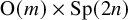 $\mathrm {O}(m) \times \mathrm {Sp}(2n)$
that has determinant
$\mathrm {O}(m) \times \mathrm {Sp}(2n)$
that has determinant
 $-1$
and hence is not in the identity component. This will be needed in order for the incarnation functor defined in Section 8 to be full.
$-1$
and hence is not in the identity component. This will be needed in order for the incarnation functor defined in Section 8 to be full.
Remark 5.5. When m and n are both nonzero, there exist various distinct super Satake diagrams corresponding to the supersymmetric pair
 $(\mathfrak {gl}(m|2n), \mathfrak {osp}(m|2n))$
; see [Reference Shen and WangSW25, Ex. 2.16] for a complete list of possible choices. Although we have made a specific choice in (5.23), we expect that all the results in this manuscript can be developed in a parallel fashion for other choices of Satake diagrams. The precise relationship between the iquantum enveloping algebras arising from different Satake diagrams remains unclear, though they are expected to be isomorphic as superalgebras. A uniform framework encompassing all choices could potentially be realized via a general theory of the universal K-matrix in the super case, following the approach of [Reference Bao and WangBW18, Reference Balagović and KolbBK19] in the nonsuper case; see also Remark 6.5. A step in this direction was taken in [Reference Shen and WangSW25, §6], where the quasi K-matrix was constructed for general quantum supersymmetric pairs. Motivated by this philosophy, we formulate many of our arguments in Section 6 and beyond in a way that avoids reliance on any particular choice of Satake diagram.
$(\mathfrak {gl}(m|2n), \mathfrak {osp}(m|2n))$
; see [Reference Shen and WangSW25, Ex. 2.16] for a complete list of possible choices. Although we have made a specific choice in (5.23), we expect that all the results in this manuscript can be developed in a parallel fashion for other choices of Satake diagrams. The precise relationship between the iquantum enveloping algebras arising from different Satake diagrams remains unclear, though they are expected to be isomorphic as superalgebras. A uniform framework encompassing all choices could potentially be realized via a general theory of the universal K-matrix in the super case, following the approach of [Reference Bao and WangBW18, Reference Balagović and KolbBK19] in the nonsuper case; see also Remark 6.5. A step in this direction was taken in [Reference Shen and WangSW25, §6], where the quasi K-matrix was constructed for general quantum supersymmetric pairs. Motivated by this philosophy, we formulate many of our arguments in Section 6 and beyond in a way that avoids reliance on any particular choice of Satake diagram.
5.4 Modules over the iquantum enveloping superalgebra
We have a restriction functor
 $$\begin{align*}\operatorname{\mathrm{Res}} \colon \mathrm{U}_\sigma\text{-tmod} \to \mathrm{U}^\imath_\sigma\text{-tmod}. \end{align*}$$
When there is no chance for confusion, we will sometimes continue to denote
 $\operatorname {\mathrm {Res}}(V^\pm )$
by
$\operatorname {\mathrm {Res}}(V^\pm )$
by
 $V^\pm $
. Direct computation using (5.15), (5.16), (5.27), and (5.28) shows that the actions of
$V^\pm $
. Direct computation using (5.15), (5.16), (5.27), and (5.28) shows that the actions of
 $B_i$
,
$B_i$
,
 $i\in I_\circ $
, on
$i\in I_\circ $
, on
 $V^+$
and
$V^+$
and
 $V^-$
are given by
$V^-$
are given by
 $$ \begin{align} B_i v^+_j = \begin{cases} v_{j+1}^+ & \text{if } j=i, \\ - q \varsigma_i v_{j-3}^+ & \text{if } i<0,\ j=i+2, \\ - q \varsigma_0 v_{-1}^+ & \text{if } i=0,\ j=1, \\ q \varsigma_i v_{j-1}^+ & \text{if } i>0,\ j=i+1, \\ 0 & \text{otherwise}, \end{cases} \quad B_i v^-_j = \begin{cases} (-1)^{\delta_{i,0}} v_{j-1}^- & \text{if } j=i+1, \\ - q \varsigma_i v_{j+3}^- & \text{if } i<0,\ j=i-1, \\ - q \varsigma_0 v_1^- & \text{if } i=0,\ j=-1, \\ q \varsigma_i v_{j+1}^- & \text{if } i>0,\ j=i, \\ 0 & \text{otherwise}. \end{cases} \end{align} $$
Define the involution
 $$ \begin{align} \phi \colon I_V \to I_V,\quad \phi(i) = i - \delta_{i \le 0} (-1)^i = \begin{cases} i, & i>0, \\ i-1, & i \in \{0,-2,-4,\dotsc,2-2n\}, \\ i+1, & i \in \{-1,-3,-5,\dotsc,1-2n\}. \end{cases} \end{align} $$
For
 $i \in I_V$
, define
$i \in I_V$
, define
 $$ \begin{align} \tilde{\varsigma}_i := \begin{cases} \prod_{k=1}^{i-1} (q \varsigma_k)^{-1}, & i> 0, \\ \prod_{k = \lfloor \frac{i+1}{2} \rfloor}^0 (-q \varsigma_{2k}), & i \le 0. \end{cases} \end{align} $$
Note that
 $\tilde {\varsigma }_{\phi (i)} = \tilde {\varsigma }_i$
for all
$\tilde {\varsigma }_{\phi (i)} = \tilde {\varsigma }_i$
for all
 $i \in I_V.$
Lemma 5.6. The linear map
 $\varphi \colon V^- \to V^+$
determined by
$\varphi \colon V^- \to V^+$
determined by
 $$ \begin{align} \varphi(v_i^-) = \tilde{\varsigma}_i v_{\phi(i)}^+ \end{align} $$
is a
 $\mathrm {U}^\imath _\sigma $
-module isomorphism. Its inverse is determined by
$\mathrm {U}^\imath _\sigma $
-module isomorphism. Its inverse is determined by
 $\varphi ^{-1}(v_i^+) = \tilde {\varsigma }_i^{-1} v_{\phi (i)}^-$
.
$\varphi ^{-1}(v_i^+) = \tilde {\varsigma }_i^{-1} v_{\phi (i)}^-$
.
Proof. This follows from a direct computation using (5.30).
Lemma 5.7. The
 $\mathrm {U}^\imath _\sigma $
-modules
$\mathrm {U}^\imath _\sigma $
-modules
 $V^+$
and
$V^+$
and
 $V^-$
are simple.
$V^-$
are simple.
Proof. By Lemma 5.6, it suffices to show that
 $V^+$
is simple. Suppose M is a nonzero submodule of
$V^+$
is simple. Suppose M is a nonzero submodule of
 $V^+$
. Since
$V^+$
. Since
 $V^+$
is generated by
$V^+$
is generated by
 $v_m^+$
, to show that
$v_m^+$
, to show that
 $M=V^+$
, it suffices to show that
$M=V^+$
, it suffices to show that
 $v_m^+ \in M$
. Let v be a nonzero element of M. If
$v_m^+ \in M$
. Let v be a nonzero element of M. If
 $v=v_m^+$
, we are done. Otherwise, multiplying by a nonzero scalar if necessary, we may assume
$v=v_m^+$
, we are done. Otherwise, multiplying by a nonzero scalar if necessary, we may assume
 $$\begin{align*}v = v_i^+ + \sum_{j>i} c_j v_j^+ \end{align*}$$
for some
 $i \in I_V$
,
$i \in I_V$
,
 $i<m$
, and
$i<m$
, and
 $c_j \in \Bbbk $
. If
$c_j \in \Bbbk $
. If
 $i<m-1$
, then, by (5.30), we have
$i<m-1$
, then, by (5.30), we have
 $$\begin{align*}B_{m-1} B_{m-2} \dotsm B_{i+1} B_i v = v_m^+, \end{align*}$$
where we interpret
 $B_{2k-1}$
as
$B_{2k-1}$
as
 $F_{2k-1}$
for
$F_{2k-1}$
for
 $k \le 0$
. On the other hand, if
$k \le 0$
. On the other hand, if
 $i=m-1$
, then
$i=m-1$
, then
 $v = v_{m-1}^+ + c_m v_m^+$
. First suppose
$v = v_{m-1}^+ + c_m v_m^+$
. First suppose
 $c_m \ne 0$
. If
$c_m \ne 0$
. If
 $m>0$
, we have
$m>0$
, we have
 $$\begin{align*}(1-\sigma)v = 2 v_m^+. \end{align*}$$
If
 $m=0$
, we have
$m=0$
, we have
 $$\begin{align*}B_{-1} v = v_0^+. \end{align*}$$
Finally, if
 $c_m = 0$
, then
$c_m = 0$
, then
 $B_{m-1} v = B_{m-1} v_{m-1}^+ = v_m^+$
. In all cases, we have shown that
$B_{m-1} v = B_{m-1} v_{m-1}^+ = v_m^+$
. In all cases, we have shown that
 $v_m^+ \in M$
.
$v_m^+ \in M$
.
6 Incarnation functors
In this section we relate the diagrammatic categories of Section 2 to the representation theory of
 $\mathrm {U}^\imath $
. Throughout this section, we work over the field
$\mathrm {U}^\imath $
. Throughout this section, we work over the field
 $\Bbbk = \mathbb {C}(q)$
.
$\Bbbk = \mathbb {C}(q)$
.
6.1 The oriented incarnation functor
The following proposition is known to experts. However, since we could not locate a proof in the literature, we have included one.
Proposition 6.1. There is a unique
 $\Bbbk $
-linear monoidal functor
$\Bbbk $
-linear monoidal functor ![]() given on objects by
given on objects by
 ${\mathord {\uparrow }} \mapsto V^+$
,
${\mathord {\uparrow }} \mapsto V^+$
,
 ${\mathord {\downarrow }} \mapsto V^-$
, and on morphisms by
${\mathord {\downarrow }} \mapsto V^-$
, and on morphisms by
Proof. We must show that ![]() respects the relations (2.1) to (2.4). The first three equalities in (2.1) follow immediately from the fact that
respects the relations (2.1) to (2.4). The first three equalities in (2.1) follow immediately from the fact that
 $T_{++}$
is the action of the braiding on
$T_{++}$
is the action of the braiding on
 $V^+ \otimes V^+$
. Furthermore, it follows from (2.5) that
$V^+ \otimes V^+$
. Furthermore, it follows from (2.5) that ![]() and
and ![]() are the components of the braiding on
are the components of the braiding on
 $V^+ \otimes V^-$
and
$V^+ \otimes V^-$
and
 $V^- \otimes V^+$
, respectively. Indeed, if X and Y are objects in a rigid braided monoidal category, and
$V^- \otimes V^+$
, respectively. Indeed, if X and Y are objects in a rigid braided monoidal category, and
 $X^*$
is the dual of X, then naturality of the braiding implies that
$X^*$
is the dual of X, then naturality of the braiding implies that

Tensoring on the left with
 $X^*$
, then composing on the bottom with
$X^*$
, then composing on the bottom with

and using the adjunction relation, gives

This shows that ![]() is the braiding on
is the braiding on
 $V^+ \otimes V^-$
. The argument for
$V^+ \otimes V^-$
. The argument for ![]() is analogous. Then the last two equalities in (2.1) follow from the properties of a braided monoidal category.
is analogous. Then the last two equalities in (2.1) follow from the properties of a braided monoidal category.
The fact that ![]() respects (2.2) follows easily from (5.21) and (5.22). For the first relation in (2.3), first note that, since
respects (2.2) follows easily from (5.21) and (5.22). For the first relation in (2.3), first note that, since
 $V^+$
is simple, we have
$V^+$
is simple, we have
 $\dim _\Bbbk \operatorname {\mathrm {End}}_{\mathrm {U}}(V^+) = 1$
. Thus, there exists
$\dim _\Bbbk \operatorname {\mathrm {End}}_{\mathrm {U}}(V^+) = 1$
. Thus, there exists
 $c \in \Bbbk $
such that
$c \in \Bbbk $
such that

Using (5.18) to (5.21), we compute that the action of the left-hand side of (6.1) on
 $v_{1-n}^+$
is given by
$v_{1-n}^+$
is given by

Thus,
 $c=q^{m-n}$
, as desired. The proof that
$c=q^{m-n}$
, as desired. The proof that ![]() respects the second equality in (2.3) is similar.
respects the second equality in (2.3) is similar.
To show that ![]() respects the last relation in (2.3), we compute that
respects the last relation in (2.3), we compute that

as desired.
The verification that ![]() respects (2.4) is a standard direct verification.
respects (2.4) is a standard direct verification.
The following result will be used in the proof of Theorem 6.4.
Lemma 6.2. We have


As explained in the first paragraph of the proof of Proposition 6.1, the
 $V^+ \otimes V^-$
and
$V^+ \otimes V^-$
and
 $V^- \otimes V^-$
components of the braiding on
$V^- \otimes V^-$
components of the braiding on
 $\mathrm {U}\text {-tmod}$
are
$\mathrm {U}\text {-tmod}$
are
6.2 The disoriented incarnation functor
The composition of functors
endows
 $\mathrm {U}^\imath _\sigma \text {-tmod}$
with the structure of a right
$\mathrm {U}^\imath _\sigma \text {-tmod}$
with the structure of a right ![]() -module category.
-module category.
The following lemma will allow us to simplify an argument in the proof of Theorem 6.4.
Lemma 6.3. As a
 $\mathrm {U}^\imath $
-module (hence, also as a
$\mathrm {U}^\imath $
-module (hence, also as a
 $\mathrm {U}^\imath _\sigma $
-module),
$\mathrm {U}^\imath _\sigma $
-module),
 $\operatorname {\mathrm {Res}}(V^- \otimes V^-)$
is generated by
$\operatorname {\mathrm {Res}}(V^- \otimes V^-)$
is generated by
 $$ \begin{align} \{v_i^-\otimes v_j^- : \phi(i)\neq j\} \cup \{v_i^-\otimes v_i^-: i>0\}. \end{align} $$
Proof. Let W be the
 $\mathrm {U}^\imath $
-submodule generated by the given vectors. By the definition (5.31) of
$\mathrm {U}^\imath $
-submodule generated by the given vectors. By the definition (5.31) of
 $\phi $
, it suffices to show that
$\phi $
, it suffices to show that
 $$ \begin{align} v_{-2k}^- \otimes v_{-2k-1}^- \in W \quad \text{and} \quad v_{-2k-1}^- \otimes v_{-2k}^- \in W \end{align} $$
for
 $0 \le k \le n-1$
. We prove this by induction on k.
$0 \le k \le n-1$
. We prove this by induction on k.
 $$\begin{align*}B_0 = F_0 + \varsigma_0 (E_{-1}E_0-qE_0E_{-1}) K_0^{-1}. \end{align*}$$
Thus
 $$\begin{align*}B_0(v_{-1}^-\otimes v_1^-) \overset{(5.9)}{\underset{(5.16)}{=}} - v_{-1}^-\otimes v_0^- - \varsigma_0 v_1^-\otimes v_1^-. \end{align*}$$
Since
 $v_{-1}^-\otimes v_1^-,v_1^-\otimes v_1^-\in W$
, we conclude that
$v_{-1}^-\otimes v_1^-,v_1^-\otimes v_1^-\in W$
, we conclude that
 $v_{-1}^-\otimes v_0^-\in W$
. On the other hand, we have
$v_{-1}^-\otimes v_0^-\in W$
. On the other hand, we have
 $$\begin{align*}E_{-1}(v_{-1}^-\otimes v_{-1}^-) \overset{(5.9)}{=} (E_{-1}\otimes 1+K_{-1}\otimes E_{-1})(v_{-1}^-\otimes v_{-1}^-)=v_0^-\otimes v_{-1}^-+qv_{-1}^-\otimes v_0^-. \end{align*}$$
Since
 $v_{-1}^-\otimes v_{-1}^-\in W$
, we see that
$v_{-1}^-\otimes v_{-1}^-\in W$
, we see that
 $v_0^-\otimes v_{-1}^-\in W$
. Thus, (6.4) holds for
$v_0^-\otimes v_{-1}^-\in W$
. Thus, (6.4) holds for
 $k=0$
.
$k=0$
.
Next suppose that
 $1 \le k \le n-1$
and that (6.4) holds for
$1 \le k \le n-1$
and that (6.4) holds for
 $k-1$
. Let
$k-1$
. Let
 $\mathrm {U} = \bigoplus _{\alpha \in X} \mathrm {U}_\alpha $
be the usual grading on
$\mathrm {U} = \bigoplus _{\alpha \in X} \mathrm {U}_\alpha $
be the usual grading on
 $\mathrm {U}$
by the root lattice and, for
$\mathrm {U}$
by the root lattice and, for
 $M \in \mathrm {U}\text {-tmod}$
and a weight
$M \in \mathrm {U}\text {-tmod}$
and a weight
 $\mu $
, let
$\mu $
, let
 $M_\mu $
denote the
$M_\mu $
denote the
 $\mu $
-weight space of M. Note that
$\mu $
-weight space of M. Note that
 $$\begin{align*}B_{-2k} \in F_{-2k} + \mathrm{U}_{\epsilon_{-2k-1}-\epsilon_{-2k+2}}. \end{align*}$$
Since
 $$\begin{align*}F_{-2k}(v_{-2k+1}^-\otimes v_{-2k-1}^-) \overset{(5.9)}{=} (F_{-2k}\otimes K_{-2k}^{-1} + 1 \otimes F_{-2k})(v_{-2k+1}^- \otimes v_{-2k-1}^-) \overset{(5.16)}{=} v_{-2k+1}^-\otimes v_{-2k}^-, \end{align*}$$
we have
 $$\begin{align*}B_{-2k} (v_{-2k+1}^-\otimes v_{-2k-1}^-) \in v_{-2k+1}^-\otimes v_{-2k}^- + (V^- \otimes V^-)_{-\epsilon_{-2k+1}-\epsilon_{-2k+2}}. \end{align*}$$
Because
 $(V^- \otimes V^-)_{-\epsilon _{-2k+1}-\epsilon _{-2k+2}}$
is spanned by
$(V^- \otimes V^-)_{-\epsilon _{-2k+1}-\epsilon _{-2k+2}}$
is spanned by
 $v_{-2k+1}^- \otimes v_{-2k+2}^-$
and
$v_{-2k+1}^- \otimes v_{-2k+2}^-$
and
 $v_{-2k+2}^- \otimes v_{-2k+1}^-$
, both of which lie in W by the inductive hypothesis, we conclude that
$v_{-2k+2}^- \otimes v_{-2k+1}^-$
, both of which lie in W by the inductive hypothesis, we conclude that
 $v_{-2k+1}^-\otimes v_{-2k-1}^-\in W$
.
$v_{-2k+1}^-\otimes v_{-2k-1}^-\in W$
.
Finally, we calculate that
 $$ \begin{align*} E_{-2k+1} (v_{-2k+1}^-\otimes v_{-2k+1}^-) &\overset{(5.9)}{=} (E_{-2k+1}\otimes 1 + K_{-2k+1} \otimes E_{-2k+1})(v_{-2k+1}^-\otimes v_{-2k+1}^-) \\& \overset{(5.16)}{=} v_{-2k}^-\otimes v_{-2k+1}^- + q v_{-2k+1}^- \otimes v_{-2k}^-. \end{align*} $$
Since
 $v_{-2k+1}^- \otimes v_{-2k+1}^- \in W$
and
$v_{-2k+1}^- \otimes v_{-2k+1}^- \in W$
and
 $v_{-2k+1}^- \otimes v_{-2k}^- \in W$
, we conclude that
$v_{-2k+1}^- \otimes v_{-2k}^- \in W$
, we conclude that
 $v_{-2k}^- \otimes v_{-2k+1}^- \in W$
as well. Thus, (6.4) holds, completing the proof of the induction step.
$v_{-2k}^- \otimes v_{-2k+1}^- \in W$
as well. Thus, (6.4) holds, completing the proof of the induction step.
Theorem 6.4. There is a unique strict morphism of ![]() -modules
-modules ![]() such that
such that
Proof. The property of being a strict morphism of ![]() -modules, together with the definition (6.2), means that the diagram
-modules, together with the definition (6.2), means that the diagram

commutes, where the horizontal arrows are the right actions. It follows that ![]() is uniquely determined by (6.5), since
is uniquely determined by (6.5), since
 $B_0$
,
$B_0$
, ![]() , and
, and ![]() generate
generate ![]() as an
as an ![]() -module. In particular,
-module. In particular, ![]() . It remains to show that
. It remains to show that ![]() respects the relations (2.17) and (2.18). The first two relations in (2.17) are immediate.
respects the relations (2.17) and (2.18). The first two relations in (2.17) are immediate.
Next we verify the first relation in (2.18). The image under ![]() of the left-hand side is the map
of the left-hand side is the map

and ![]() is the map
is the map
verifying the first relation in (2.18).
Now consider the second relation in (2.18). The image under ![]() of the left-hand side is the map
of the left-hand side is the map

and ![]() is the map
is the map

verifying the second relation in (2.18).
It remains to verify the last relation in (2.17). By Lemma 6.3, it suffices to show that the images under ![]() of the two sides of the relation agree on the set (6.3). Note that
of the two sides of the relation agree on the set (6.3). Note that
 $p(\phi (i)) = p(i)$
for all
$p(\phi (i)) = p(i)$
for all
 $i \in I_V$
. Using Lemma 6.2, we compute, for
$i \in I_V$
. Using Lemma 6.2, we compute, for
 $i>0$
,
$i>0$
,

and

which agree. If
 $\phi (i) \ne j$
, then
$\phi (i) \ne j$
, then

and

which also agree since the condition
 $\phi (i) \ne j$
implies that
$\phi (i) \ne j$
implies that
 $i>j \iff \phi (i)>\phi (j)$
.
$i>j \iff \phi (i)>\phi (j)$
.
Remark 6.5. If either
 $m = 0$
or
$m = 0$
or
 $n = 0$
, then the preservation of the last relation in (2.17) under
$n = 0$
, then the preservation of the last relation in (2.17) under ![]() follows from the reflection equation [Reference Balagović and KolbBK19, (9.16)] between the universal R-matrix of
follows from the reflection equation [Reference Balagović and KolbBK19, (9.16)] between the universal R-matrix of
 $\mathrm {U}$
and the universal K-matrix of
$\mathrm {U}$
and the universal K-matrix of
 $\mathrm {U}^\imath $
. Indeed, let
$\mathrm {U}^\imath $
. Indeed, let
 $\tau _0$
be the algebra automorphism of
$\tau _0$
be the algebra automorphism of
 $\mathrm {U}$
corresponding to the nontrivial involution of its Dynkin diagram. By [Reference Balagović and KolbBK19, Cor. 7.7], the universal K-matrix
$\mathrm {U}$
corresponding to the nontrivial involution of its Dynkin diagram. By [Reference Balagović and KolbBK19, Cor. 7.7], the universal K-matrix
 $\mathcal {K}$
defines an isomorphism of
$\mathcal {K}$
defines an isomorphism of
 $\mathrm {U}^\imath $
-modules
$\mathrm {U}^\imath $
-modules
 $$\begin{align*}\mathcal{K}_M \colon M \to M^{\tau_0} \end{align*}$$
for any finite-dimensional
 $\mathrm {U}$
-module M, where
$\mathrm {U}$
-module M, where
 $M^{\tau _0}$
has the same underlying vector space as M but with the action given by
$M^{\tau _0}$
has the same underlying vector space as M but with the action given by
 $(x, v) \mapsto \tau _0(x) v$
for
$(x, v) \mapsto \tau _0(x) v$
for
 $x \in \mathrm {U}$
and
$x \in \mathrm {U}$
and
 $v \in M^{\tau _0}$
. (Recall that the diagram automorphism
$v \in M^{\tau _0}$
. (Recall that the diagram automorphism
 $\tau $
, which is part of the data of the super Satake diagram (5.23), is the identity in our case.) It follows that the universal K-matrix
$\tau $
, which is part of the data of the super Satake diagram (5.23), is the identity in our case.) It follows that the universal K-matrix
 $\mathcal {K}$
defines a
$\mathcal {K}$
defines a
 $\mathrm {U}^\imath $
-isomorphism
$\mathrm {U}^\imath $
-isomorphism
 $$\begin{align*}\mathcal{K}_{V^-} \colon V^- \to (V^-)^{\tau_0}. \end{align*}$$
However, it is straightforward to check that
 $(V^-)^{\tau _0} \cong V^+$
as
$(V^-)^{\tau _0} \cong V^+$
as
 $\mathrm {U}$
-modules. Since
$\mathrm {U}$
-modules. Since
 $V^- \cong V^+$
as
$V^- \cong V^+$
as
 $\mathrm {U}^\imath $
-modules and both are irreducible, Schur’s Lemma implies that one can identify
$\mathrm {U}^\imath $
-modules and both are irreducible, Schur’s Lemma implies that one can identify
 $\mathcal {K}_{V^-}$
with the map
$\mathcal {K}_{V^-}$
with the map
 $\varphi $
, up to a scalar. Then the last relation in (2.17) follows from the reflection equation established in [Reference Balagović and KolbBK19, (9.16)]. The proof of Theorem 6.4 could be made significantly shorter if the machinery of the K-matrix existed in the super setting; unfortunately, this is not yet the case.
$\varphi $
, up to a scalar. Then the last relation in (2.17) follows from the reflection equation established in [Reference Balagović and KolbBK19, (9.16)]. The proof of Theorem 6.4 could be made significantly shorter if the machinery of the K-matrix existed in the super setting; unfortunately, this is not yet the case.
6.3 The iquantum incarnation functor
Define
 $$\begin{align*}V_r = \operatorname{\mathrm{Res}} \left( (V^+)^{\otimes r} \right), \qquad r \in \mathbb{N}. \end{align*}$$
Proposition 6.6. The composite morphism of ![]() -modules
-modules
is given on objects by
 $\mathsf {B}_r \mapsto V_r$
,
$\mathsf {B}_r \mapsto V_r$
,
 $r \in \mathbb {N}$
, and on morphisms by
$r \in \mathbb {N}$
, and on morphisms by

Proof. This follows immediately from the definitions of ![]() and
and
 $\mathbf {G}$
.
$\mathbf {G}$
.
Note that ![]() is not a strict morphism of
is not a strict morphism of ![]() -modules, since
-modules, since
 $\mathbf {G}$
is not; see Remark 4.4. The map
$\mathbf {G}$
is not; see Remark 4.4. The map
recovers the operator
 $\Xi $
defined in [Reference Shen and WangSW25, §7.3].
$\Xi $
defined in [Reference Shen and WangSW25, §7.3].
7 Basis theorems and endomorphism algebras
In this section, we describe bases for the morphism spaces of ![]() and
and ![]() . Throughout this section
. Throughout this section
 $\Bbbk $
is an arbitrary integral domain and
$\Bbbk $
is an arbitrary integral domain and
 $q,t$
are elements of
$q,t$
are elements of
 $\Bbbk ^\times $
such that
$\Bbbk ^\times $
such that
 $t-t^{-1}$
is divisible by
$t-t^{-1}$
is divisible by
 $q-q^{-1}$
.
$q-q^{-1}$
.
7.1 Basis theorem
For
 $\lambda ,\mu \in \langle {\mathord {\uparrow }},{\mathord {\downarrow }} \rangle $
, a
$\lambda ,\mu \in \langle {\mathord {\uparrow }},{\mathord {\downarrow }} \rangle $
, a
 $(\lambda ,\mu )$
-matching is a partition of the set
$(\lambda ,\mu )$
-matching is a partition of the set
 $$\begin{align*}E(\lambda,\mu) := \{-1,-2,\dotsc,-\ell(\lambda),1,2,\dotsc,\ell(\mu)\} \end{align*}$$
into subsets of size two. In a string diagram representing a morphism in ![]() , each nonclosed string has two endpoints. We view these endpoints as elements of
, each nonclosed string has two endpoints. We view these endpoints as elements of
 $E(\lambda ,\mu )$
by numbering the
$E(\lambda ,\mu )$
by numbering the
 ${\mathord {\uparrow }}$
,
${\mathord {\uparrow }}$
,
 ${\mathord {\downarrow }}$
in
${\mathord {\downarrow }}$
in
 $\lambda $
by
$\lambda $
by
 $-1,-2,\dotsc ,-\ell (\lambda )$
from left to right and the
$-1,-2,\dotsc ,-\ell (\lambda )$
from left to right and the
 ${\mathord {\uparrow }}$
,
${\mathord {\uparrow }}$
,
 ${\mathord {\downarrow }}$
in
${\mathord {\downarrow }}$
in
 $\mu $
by
$\mu $
by
 $1,2,\dotsc ,\ell (\mu )$
from left to right. A reduced
$1,2,\dotsc ,\ell (\mu )$
from left to right. A reduced
 $(\lambda ,\mu )$
-diagram for a given
$(\lambda ,\mu )$
-diagram for a given
 $(\lambda ,\mu )$
-matching is a string diagram representing a morphism in
$(\lambda ,\mu )$
-matching is a string diagram representing a morphism in ![]() such that:
such that:
-
• the endpoints of each string correspond under the given matching (i.e., they form one of the two-element subsets of the partition);
-
• there are no closed strings (i.e., strings with no endpoints);
-
• no string has more than one critical point (i.e., more than one point at which the tangent is horizontal);
-
• there are no self-intersections of strings and no two strings cross each other more than once;
-
• all toggles on strings connecting the top and bottom of the diagram are near their bottom endpoint;
-
• all toggles on strings with both endpoints at the top of the diagram or both endpoints at the bottom of the diagram are near the left endpoint of the string.
For example, for
 $\lambda = {\mathord {\downarrow }} {\mathord {\uparrow }} {\mathord {\downarrow }} {\mathord {\downarrow }} {\mathord {\downarrow }} {\mathord {\uparrow }} {\mathord {\uparrow }}$
and
$\lambda = {\mathord {\downarrow }} {\mathord {\uparrow }} {\mathord {\downarrow }} {\mathord {\downarrow }} {\mathord {\downarrow }} {\mathord {\uparrow }} {\mathord {\uparrow }}$
and
 $\mu = {\mathord {\uparrow }} {\mathord {\uparrow }} {\mathord {\uparrow }} {\mathord {\uparrow }} {\mathord {\downarrow }}$
,
$\mu = {\mathord {\uparrow }} {\mathord {\uparrow }} {\mathord {\uparrow }} {\mathord {\uparrow }} {\mathord {\downarrow }}$
,

is a reduced
 $(\lambda ,\mu )$
-diagram for the
$(\lambda ,\mu )$
-diagram for the
 $(\lambda ,\mu )$
-matching
$(\lambda ,\mu )$
-matching
 $$\begin{align*}\big\{ \{-1,-5\}, \{-2,1\}, \{-3,4\}, \{-4,-7\}, \{-6,5\}, \{2,3\} \big\}. \end{align*}$$
Fix a set ![]() consisting of a choice of reduced
consisting of a choice of reduced
 $(\lambda ,\mu )$
-diagram for each of the
$(\lambda ,\mu )$
-diagram for each of the
 $(\lambda ,\mu )$
-matchings.
$(\lambda ,\mu )$
-matchings.
Theorem 7.1. For objects ![]() , the morphism space
, the morphism space ![]() is a free
is a free
 $\Bbbk $
-module with basis
$\Bbbk $
-module with basis ![]() .
.
Proof. Set ![]() . It suffices to consider the ground ring
. It suffices to consider the ground ring
 $$\begin{align*}\Bbbk = \mathbb{Z}[q^{\pm 1}, t^{\pm 1}, (t-t^{-1})/(q-q^{-1})], \end{align*}$$
since the more general case then follows by base extension. The defining relations and the additional relations deduced in Sections 2.1 and 2.2 give Reidemeister-type relations modulo terms with fewer crossings, plus a skein relation. The relation (2.25), together with the skein relation (2.2), implies that we can slide toggles through crossings, modulo diagrams with fewer crossings. Furthermore, we can slide toggles over cups and caps, modulo diagrams with fewer crossings, by moving cups and caps to the left of the diagram, then using (2.25) and (2.26). These relations allow us to transform diagrams for morphisms in ![]() in way similar to the way oriented tangles are simplified in skein categories, modulo diagrams with fewer crossings. Therefore, there is a straightening algorithm to rewrite any diagram representing a morphism
in way similar to the way oriented tangles are simplified in skein categories, modulo diagrams with fewer crossings. Therefore, there is a straightening algorithm to rewrite any diagram representing a morphism
 $\lambda \to \mu $
as a linear combination of the ones in
$\lambda \to \mu $
as a linear combination of the ones in ![]() .
.
It remains to prove linear independence. For
 $\mu \in \langle {\mathord {\uparrow }},{\mathord {\downarrow }} \rangle $
, let
$\mu \in \langle {\mathord {\uparrow }},{\mathord {\downarrow }} \rangle $
, let
 $\mu '$
denote the word obtained from
$\mu '$
denote the word obtained from
 $\mu $
by rotating
$\mu $
by rotating
. For example,
 $({\mathord {\uparrow }} {\mathord {\uparrow }} {\mathord {\downarrow }} {\mathord {\uparrow }} {\mathord {\downarrow }})' = ({\mathord {\uparrow }} {\mathord {\downarrow }} {\mathord {\uparrow }} {\mathord {\downarrow }} {\mathord {\downarrow }})$
. For
$({\mathord {\uparrow }} {\mathord {\uparrow }} {\mathord {\downarrow }} {\mathord {\uparrow }} {\mathord {\downarrow }})' = ({\mathord {\uparrow }} {\mathord {\downarrow }} {\mathord {\uparrow }} {\mathord {\downarrow }} {\mathord {\downarrow }})$
. For
 $\lambda , \mu \in \langle {\mathord {\uparrow }},{\mathord {\downarrow }} \rangle $
, we have a
$\lambda , \mu \in \langle {\mathord {\uparrow }},{\mathord {\downarrow }} \rangle $
, we have a
 $\Bbbk $
-linear isomorphism
$\Bbbk $
-linear isomorphism

with inverse

Via the straightening algorithm mentioned above (e.g., using (2.4) to remove instances of multiple critical points and (2.2) to flip crossings if necessary), there is a bijection from ![]() to
to ![]() such that (7.1) acts by this bijection modulo diagrams with fewer crossings. Thus, it suffices to prove the linear independence of
such that (7.1) acts by this bijection modulo diagrams with fewer crossings. Thus, it suffices to prove the linear independence of ![]() . Since
. Since ![]() when
when
 $\ell (\lambda ) \notin 2\mathbb {N}$
, we assume that
$\ell (\lambda ) \notin 2\mathbb {N}$
, we assume that
 $\ell (\lambda ) \in 2\mathbb {N}$
.
$\ell (\lambda ) \in 2\mathbb {N}$
.
We will use the disoriented incarnation functor ![]() in the case that
in the case that
 $n=0$
, which we assume throughout this proof. We also make the choice (5.29) for the
$n=0$
, which we assume throughout this proof. We also make the choice (5.29) for the
 $\varsigma _i$
. This implies that
$\varsigma _i$
. This implies that
 $\tilde {\varsigma }_i = 1$
for all
$\tilde {\varsigma }_i = 1$
for all
 $i \in I_V$
; see (5.32).
$i \in I_V$
; see (5.32).
For
 $\mu \in \langle {\mathord {\uparrow }},{\mathord {\downarrow }} \rangle $
and
$\mu \in \langle {\mathord {\uparrow }},{\mathord {\downarrow }} \rangle $
and
 $1 \le a \le \ell (\mu )$
, let
$1 \le a \le \ell (\mu )$
, let
 $$ \begin{align} \pi_a(\mu) = \begin{cases} + &\text{if the } a\, \text{ th term in } \mu \text{ is } {\mathord{\uparrow}}, \\ - &\text{if the } a\, \text{ th term in } \mu \text{ is } {\mathord{\downarrow}}. \end{cases} \end{align} $$
Then, for
 $\mathbf {i} = (i_1,\dotsc ,i_{\ell (\mu )}) \in I_V^{\ell (\mu )}$
, let
$\mathbf {i} = (i_1,\dotsc ,i_{\ell (\mu )}) \in I_V^{\ell (\mu )}$
, let
We define

For a morphism
 $f \colon \mu \to \nu $
in
$f \colon \mu \to \nu $
in ![]() , define
, define
Let J be the ideal of
 $\mathbb {Z}[q^{\pm 1}]$
generated by
$\mathbb {Z}[q^{\pm 1}]$
generated by
 $q-1$
. It follows from (5.21) and (5.22) that, for
$q-1$
. It follows from (5.21) and (5.22) that, for
 $\mu ,\nu \in \langle {\mathord {\uparrow }},{\mathord {\downarrow }} \rangle $
,
$\mu ,\nu \in \langle {\mathord {\uparrow }},{\mathord {\downarrow }} \rangle $
,

and

where
 $\operatorname {\mathrm {flip}} \colon u \otimes w \to w \otimes u$
is the tensor flip. Similarly, the other crossings also induce the flip map. Thus, using also (5.17), (5.18), and (5.33), we see that, for
$\operatorname {\mathrm {flip}} \colon u \otimes w \to w \otimes u$
is the tensor flip. Similarly, the other crossings also induce the flip map. Thus, using also (5.17), (5.18), and (5.33), we see that, for ![]() and
and
 $\mathbf {i} = (i_1,\dotsc ,i_{\ell (\lambda )}) \in I_V^{\ell (\lambda )}$
,
$\mathbf {i} = (i_1,\dotsc ,i_{\ell (\lambda )}) \in I_V^{\ell (\lambda )}$
,

Now suppose that
 $m \ge \ell (\lambda )$
and that
$m \ge \ell (\lambda )$
and that

Then, for each ![]() , evaluating (7.3) at
, evaluating (7.3) at
 $v_{\mathbf {i},\lambda }$
for some
$v_{\mathbf {i},\lambda }$
for some
 $\mathbf {i}$
whose entries are equal if and only if they are matched under the matching corresponding to f shows that
$\mathbf {i}$
whose entries are equal if and only if they are matched under the matching corresponding to f shows that
 $\gamma _f = 0$
. Thus, the
$\gamma _f = 0$
. Thus, the ![]() ,
, ![]() , are linearly independent if
, are linearly independent if
 $m \ge \ell (\lambda )$
.
$m \ge \ell (\lambda )$
.
Now suppose that
 $\lambda \in \langle {\mathord {\uparrow }},{\mathord {\downarrow }} \rangle $
and that
$\lambda \in \langle {\mathord {\uparrow }},{\mathord {\downarrow }} \rangle $
and that

Multiplying by an appropriate power of
 $(q-q^{-1})$
, we may assume that
$(q-q^{-1})$
, we may assume that
 $c_f(q,t) \in \mathbb {Z}[q^{\pm 1}, t^{\pm 1}]$
for all
$c_f(q,t) \in \mathbb {Z}[q^{\pm 1}, t^{\pm 1}]$
for all ![]() . Applying
. Applying ![]() , we have
, we have

Since the ![]() ,
, ![]() , are linearly independent, we have
, are linearly independent, we have
 $c_f(q,q^m)=0$
for all
$c_f(q,q^m)=0$
for all ![]() and
and
 $m \ge \ell (\lambda )$
. As there are infinitely many choices of m, it follows that
$m \ge \ell (\lambda )$
. As there are infinitely many choices of m, it follows that
 $c_f(q,t)=0$
for all f. Thus, the set
$c_f(q,t)=0$
for all f. Thus, the set ![]() is linearly independent, as desired.
is linearly independent, as desired.
For
 $r,s \in \mathbb {N}$
, define
$r,s \in \mathbb {N}$
, define
Corollary 7.2. For
 $r,s \in \mathbb {N}$
, the morphism space
$r,s \in \mathbb {N}$
, the morphism space ![]() is a free
is a free
 $\Bbbk $
-module with basis
$\Bbbk $
-module with basis ![]() .
.
Proof. This follows immediately from Theorem 4.5.
Let
 $A \subseteq \mathbb {C}(q) = \Bbbk $
be the
$A \subseteq \mathbb {C}(q) = \Bbbk $
be the
 $\mathbb {C}$
-subalgebra of rational functions regular at
$\mathbb {C}$
-subalgebra of rational functions regular at
 $q=1$
. This is a local ring with maximal ideal
$q=1$
. This is a local ring with maximal ideal
 $\mathfrak {m} = A(q-1)$
. In what follows, we identify
$\mathfrak {m} = A(q-1)$
. In what follows, we identify
 $\mathbb {C}$
with
$\mathbb {C}$
with
 $A/\mathfrak {m}$
. For
$A/\mathfrak {m}$
. For
 $d \in \mathbb {C}$
, let
$d \in \mathbb {C}$
, let ![]() denote the Brauer category, as described in [Reference Lehrer and ZhangLZ15, Th. 2.6].
denote the Brauer category, as described in [Reference Lehrer and ZhangLZ15, Th. 2.6].
Corollary 7.3. There is an isomorphism of
 $\mathbb {C}$
-linear categories from
$\mathbb {C}$
-linear categories from ![]() to the Brauer category
to the Brauer category ![]() given by
given by
Proof. It is straightforward to verify that the given functor is well defined (that is, the relations in Definition 2.7 are satisfied). It follows from [Reference Lehrer and ZhangLZ15, Th. 2.6] that, for each
 $r,s \in \mathbb {N}$
the image of
$r,s \in \mathbb {N}$
the image of ![]() under the above functor is a basis of
under the above functor is a basis of ![]() . Here we use the fact that
. Here we use the fact that

and similarly for the other diagrams in ![]() appearing in (4.4) and (4.5). It follows that the functor in the statement of the lemma is an isomorphism.
appearing in (4.4) and (4.5). It follows that the functor in the statement of the lemma is an isomorphism.
7.2 Endomorphism algebras
For
 $r \in \mathbb {N}$
, the iquantum Brauer algebra
$r \in \mathbb {N}$
, the iquantum Brauer algebra
 $\mathrm {B}_r(q,t)$
is the associative
$\mathrm {B}_r(q,t)$
is the associative
 $\Bbbk $
-algebra with generators
$\Bbbk $
-algebra with generators
 $\sigma _1,\sigma _2,\dotsc ,\sigma _{r-1}$
and e, subject to the relations
$\sigma _1,\sigma _2,\dotsc ,\sigma _{r-1}$
and e, subject to the relations
 $$ \begin{align*} \begin{gathered}\sigma_i \sigma_{i+1} \sigma_i = \sigma_{i+1} \sigma_i \sigma_{i+1},\qquad 1 \le i \le r-2, \\ \sigma_i \sigma_j = \sigma_j \sigma_i,\qquad 1 \le i,j \le r-1,\ |i-j|>1, \\ \sigma_i^2 = (q-q^{-1}) \sigma_i + 1,\qquad 1 \le i \le r-1, \\ e^2 = \frac{t-t^{-1}}{q-q^{-1}} e, \\ e \sigma_1 = \sigma_1 e = q e,\quad e \sigma_2 e = t e,\quad e \sigma_i = \sigma_i e,\qquad i > 2, \\ \sigma_2 \sigma_3 \sigma_1^{-1} \sigma_2^{-1} e_{(2)} = e_{(2)} = e_{(2)} \sigma_2 \sigma_3 \sigma_1^{-1} \sigma_2^{-1}, \quad \text{where } e_{(2)} = e \sigma_2 \sigma_3 \sigma_1^{-1} \sigma_2^{-1} e. \end{gathered}\end{align*} $$
Remark 7.4. The algebra
 $\mathrm {B}_r(q,t)$
is isomorphic to the algebra
$\mathrm {B}_r(q,t)$
is isomorphic to the algebra
 $Br_r(t^2,q^2)$
of [Reference WenzlWen12, §3.1] via the map
$Br_r(t^2,q^2)$
of [Reference WenzlWen12, §3.1] via the map
 $$\begin{align*}\mathrm{B}_r(q,t) \to Br_r(t^2,q^2),\qquad e \mapsto qt^{-1} e,\quad \sigma_i \mapsto q^{-1} g_i,\quad 1 \le i \le r-1, \end{align*}$$
as can be checked by direct verification of the defining relations. Similar algebras appeared previously in [Reference MolevMol03, Def. 2.1]. The algebras
 $\mathrm {B}_r(q,t)$
have been called q-Brauer algebras in the literature, presumably because some authors view them as deformations of Brauer algebras and the notation used for the deformation parameter is often q. We prefer the term iquantum Brauer algebras to avoid possible confusion with Birman–Murakami–Wenzl (BMW) algebras, which are also deformations of Brauer algebras, and also to avoid terminology involving notation.
$\mathrm {B}_r(q,t)$
have been called q-Brauer algebras in the literature, presumably because some authors view them as deformations of Brauer algebras and the notation used for the deformation parameter is often q. We prefer the term iquantum Brauer algebras to avoid possible confusion with Birman–Murakami–Wenzl (BMW) algebras, which are also deformations of Brauer algebras, and also to avoid terminology involving notation.
Proposition 7.5. For all
 $r \in \mathbb {N}$
and
$r \in \mathbb {N}$
and
 $\lambda \in \langle {\mathord {\uparrow }},{\mathord {\downarrow }} \rangle $
with
$\lambda \in \langle {\mathord {\uparrow }},{\mathord {\downarrow }} \rangle $
with
 $\ell (\lambda )=r$
, we have isomorphisms of algebras
$\ell (\lambda )=r$
, we have isomorphisms of algebras
Proof. By Theorem 4.5, it suffices to prove the result for ![]() . It is straightforward to verify that the map
. It is straightforward to verify that the map ![]() given by
given by

satisfies the defining relations of
 $\mathrm {B}_r(q,t)$
. It then follows from the basis theorems [Reference WenzlWen12, Th. 3.8] and Corollary 7.2 that this map is in an isomorphism.
$\mathrm {B}_r(q,t)$
. It then follows from the basis theorems [Reference WenzlWen12, Th. 3.8] and Corollary 7.2 that this map is in an isomorphism.
8 Fullness of the incarnation functors
Our goal in this final section is to show that the functors ![]() and
and ![]() are full. In light of Remark 5.3, it suffices to prove this for one particular choice of the parameters
are full. In light of Remark 5.3, it suffices to prove this for one particular choice of the parameters
 $\varsigma _i$
,
$\varsigma _i$
,
 $i \in I_\circ $
. Thus, throughout this section we make the choice (5.29). This implies that
$i \in I_\circ $
. Thus, throughout this section we make the choice (5.29). This implies that
 $\tilde {\varsigma }_i = 1$
for all
$\tilde {\varsigma }_i = 1$
for all
 $i \in I_V$
; see (5.32).
$i \in I_V$
; see (5.32).
Recall that
 $A \subseteq \mathbb {C}(q)$
is the
$A \subseteq \mathbb {C}(q)$
is the
 $\mathbb {C}$
-subalgebra of rational functions regular at
$\mathbb {C}$
-subalgebra of rational functions regular at
 $q=1$
, that
$q=1$
, that
 $\mathfrak {m} = A(q-1)$
is its unique maximal ideal, and that we identify
$\mathfrak {m} = A(q-1)$
is its unique maximal ideal, and that we identify
 $\mathbb {C}$
with
$\mathbb {C}$
with
 $A/\mathfrak {m}$
. Let
$A/\mathfrak {m}$
. Let
 $\mathrm {U}^\imath _{A}$
be the A-subalgebra of
$\mathrm {U}^\imath _{A}$
be the A-subalgebra of
 $\mathrm {U}^\imath $
generated by the elements (5.24), let
$\mathrm {U}^\imath $
generated by the elements (5.24), let
 $\mathrm {U}_{\sigma ,A}^\imath $
be the A-subalgebra of
$\mathrm {U}_{\sigma ,A}^\imath $
be the A-subalgebra of
 $\mathrm {U}^\imath _\sigma $
generated by
$\mathrm {U}^\imath _\sigma $
generated by
 $\mathrm {U}^\imath _{A}$
and
$\mathrm {U}^\imath _{A}$
and
 $\sigma $
, and let
$\sigma $
, and let
 $V_A$
be the A-submodule of
$V_A$
be the A-submodule of
 $V^+$
generated by
$V^+$
generated by
 $v_i^+$
,
$v_i^+$
,
 $i \in I_V$
. Since all the coefficients appearing in (5.15) and (5.30) lie in A, we see that
$i \in I_V$
. Since all the coefficients appearing in (5.15) and (5.30) lie in A, we see that
 $V_A$
is a
$V_A$
is a
 $\mathrm {U}_{\sigma ,A}^\imath $
-module. We also have the A-bilinear map
$\mathrm {U}_{\sigma ,A}^\imath $
-module. We also have the A-bilinear map
 $$\begin{align*}\beta_A = \operatorname{\mathrm{ev}}^- \circ (\varphi^{-1} \times 1)|_{V_A \times V_A} \colon V_A \times V_A \to A. \end{align*}$$
The elements
 $v_i := v_i^+ \otimes 1$
,
$v_i := v_i^+ \otimes 1$
,
 $i \in I_V$
, form a
$i \in I_V$
, form a
 $\mathbb {C}$
-basis of
$\mathbb {C}$
-basis of
 $V_{\mathbb {C}} := V_A \otimes _A \mathbb {C}$
. We have the induced
$V_{\mathbb {C}} := V_A \otimes _A \mathbb {C}$
. We have the induced
 $\mathbb {C}$
-bilinear map
$\mathbb {C}$
-bilinear map
 $$\begin{align*}\beta_{\mathbb{C}} = \beta_A \otimes_A \mathbb{C} \colon V_{\mathbb{C}} \times V_{\mathbb{C}} \to \mathbb{C},\qquad \beta_{\mathbb{C}}(v_i, v_j) = \delta_{i,\phi(j)} (-1)^{i+p(i)}. \end{align*}$$
Instead of working with supergroups, we will work over the equivalent theory of Harish-Chandra pairs. We refer the reader to [Reference GavariniGav20] and the references cited therein for a proof of this equivalence. A brief summary, well suited to the current paper, can also be found in [Reference Samchuck-Schnarch and SavageSSS24, §3.6, §7.5]. Let
 $$ \begin{align*} G_{\text{red}}(\beta_{\mathbb{C}}) &= \{x \in \operatorname{\mathrm{Aut}}(V_{\mathbb{C}})_0 : \beta_{\mathbb{C}}(xv,xw) = \beta_{\mathbb{C}}(v,w) \text{ for all } v,w \in V\}, \\ \mathfrak{g}(\beta_{\mathbb{C}}) &= \{ x \in \operatorname{\mathrm{End}}(V_{\mathbb{C}}) : \beta_{\mathbb{C}}(xv,w) = -(-1)^{\bar{x} \bar{v}} \beta_{\mathbb{C}}(v,xw) \text{ for all } v,w \in V\}. \end{align*} $$
The pair
 $G(\beta _{\mathbb {C}}) := (G_{\text {red}}(\beta _{\mathbb {C}}), \mathfrak {g}(\beta _{\mathbb {C}}))$
is a Harish-Chandra pair. It follows from (5.31) that
$G(\beta _{\mathbb {C}}) := (G_{\text {red}}(\beta _{\mathbb {C}}), \mathfrak {g}(\beta _{\mathbb {C}}))$
is a Harish-Chandra pair. It follows from (5.31) that
 $\beta _{\mathbb {C}}$
is supersymmetric and nondegenerate. Thus, we may identify
$\beta _{\mathbb {C}}$
is supersymmetric and nondegenerate. Thus, we may identify
 $\mathfrak {g}(\beta _{\mathbb {C}})$
with
$\mathfrak {g}(\beta _{\mathbb {C}})$
with
 $\mathfrak {osp}(m|2n)$
and
$\mathfrak {osp}(m|2n)$
and
 $G(\beta _{\mathbb {C}})$
with the orthosymplectic supergroup
$G(\beta _{\mathbb {C}})$
with the orthosymplectic supergroup
 $\mathrm {OSp}(m|2n)$
.
$\mathrm {OSp}(m|2n)$
.
The action of
 $\sigma $
on
$\sigma $
on
 $V^+$
, defined in (5.15), induces an automorphism
$V^+$
, defined in (5.15), induces an automorphism
 $\sigma $
of
$\sigma $
of
 $V_{\mathbb {C}}$
. When
$V_{\mathbb {C}}$
. When
 $m>0$
, this automorphism has determinant
$m>0$
, this automorphism has determinant
 $-1$
, and so lies in the connected component of
$-1$
, and so lies in the connected component of
 $G_{\text {red}}$
not containing the identity. Thus, as explained in [Reference Samchuck-Schnarch and SavageSSS24, §3.6], for any
$G_{\text {red}}$
not containing the identity. Thus, as explained in [Reference Samchuck-Schnarch and SavageSSS24, §3.6], for any
 $r,s \in \mathbb {N}$
, we have
$r,s \in \mathbb {N}$
, we have
 $$ \begin{align} \operatorname{\mathrm{Hom}}_{\mathrm{OSp}(m|2n)}(V_{\mathbb{C}}^{\otimes r}, V_{\mathbb{C}}^{\otimes s})& = \operatorname{\mathrm{Hom}}_{\sigma,\mathfrak{osp}(m|2n)}(V_{\mathbb{C}}^{\otimes r}, V_{\mathbb{C}}^{\otimes s}) \nonumber\\& := \{f \in \operatorname{\mathrm{Hom}}_{\mathfrak{osp}(m|2n)}(V_{\mathbb{C}}^{\otimes r}, V_{\mathbb{C}}^{\otimes s}) : f(\sigma v)= \sigma f(v) \ \forall\ v \in V_{\mathbb{C}}^{\otimes r} \}. \end{align} $$
Theorem 8.1. The functors ![]() and
and ![]() are full.
are full.
Proof. To simplify notation, let ![]() and
and ![]() . By (6.6) and Corollary 4.6, it suffices to prove that
. By (6.6) and Corollary 4.6, it suffices to prove that ![]() is full. Since all the coefficients appearing in (5.18), (5.20) to (5.22), and (5.33) lie in A, we have an incarnation functor
is full. Since all the coefficients appearing in (5.18), (5.20) to (5.22), and (5.33) lie in A, we have an incarnation functor
Consider the
 $\mathbb {C}$
-algebra homomorphism
$\mathbb {C}$
-algebra homomorphism
 $$ \begin{align} \rho_{\mathbb{C}} \colon \mathrm{U}_{\sigma,A}^\imath \otimes_A \mathbb{C} \to \operatorname{\mathrm{End}}_A(V_A) \otimes_A \mathbb{C} \cong \operatorname{\mathrm{End}}_{\mathbb{C}}(V_{\mathbb{C}}) \end{align} $$
induced by the
 $\mathrm {U}_{\sigma ,A}^\imath $
-module structure on
$\mathrm {U}_{\sigma ,A}^\imath $
-module structure on
 $V_A$
. It follows from (5.15) and (5.30) that
$V_A$
. It follows from (5.15) and (5.30) that
 $$ \begin{align} \rho_{\mathbb{C}}(B_i \otimes 1) &= E_{i+1,i} + \delta_{i>0} E_{i,i+1} + \delta_{i<0} E_{i-1,i+2} + \delta_{i,0} E_{-1,1},& i \in I_\circ, \end{align} $$
 $$ \begin{align} \rho_{\mathbb{C}}(E_{2k-1} \otimes 1) &= E_{2k-1,2k},\quad \rho_{\mathbb{C}}(F_{2k-1} \otimes 1) = E_{2k,2k-1},& 1-n \le k \le 0, \end{align} $$
where
 $E_{i,j}$
is the linear map given by
$E_{i,j}$
is the linear map given by
 $E_{i,j} v_k^+ = \delta _{j,k} v_i^+$
. A direct computation shows that the elements (8.3) and (8.4) generate
$E_{i,j} v_k^+ = \delta _{j,k} v_i^+$
. A direct computation shows that the elements (8.3) and (8.4) generate
 $\mathfrak {g}(\beta _{\mathbb {C}})$
as a Lie superalgebra. Furthermore, for
$\mathfrak {g}(\beta _{\mathbb {C}})$
as a Lie superalgebra. Furthermore, for
 $r \in \mathbb {N}$
, it follows from (5.9) that the action of
$r \in \mathbb {N}$
, it follows from (5.9) that the action of
 $\mathrm {U}^\imath _{\mathbb {C}} := \mathrm {U}^\imath _{A} \otimes _A \mathbb {C}$
on
$\mathrm {U}^\imath _{\mathbb {C}} := \mathrm {U}^\imath _{A} \otimes _A \mathbb {C}$
on
 $V_{\mathbb {C}}^{\otimes r}$
is determined by the usual comultiplication for Lie superalgebras. Thus, we have an equivalence of categories
$V_{\mathbb {C}}^{\otimes r}$
is determined by the usual comultiplication for Lie superalgebras. Thus, we have an equivalence of categories
 $$\begin{align*}\mathrm{U}^\imath_{\mathbb{C}}\text{-tmod} \simeq \mathfrak{g}(\beta_{\mathbb{C}})\text{-tmod}. \end{align*}$$
Together with (8.1), this implies that we have an equivalence of categories
 $$\begin{align*}\mathrm{U}_{\sigma,\mathbb{C}}^\imath\text{-tmod} \simeq \mathrm{OSp}(m|2n)\text{-tmod}. \end{align*}$$
The above discussion shows that we have a commutative diagram of functors

where the left vertical map is the isomorphism of Corollary 7.3 and ![]() is the monoidal incarnation functor of [Reference Lehrer and ZhangLZ17, Th. 5.4] determined by
is the monoidal incarnation functor of [Reference Lehrer and ZhangLZ17, Th. 5.4] determined by
(Here we used the fact that
 $T_{++} \otimes _A 1 = \operatorname {\mathrm {flip}}$
, which follows easily from (5.21).) By [Reference Lehrer and ZhangLZ17, Thm. 5.6], the functor
$T_{++} \otimes _A 1 = \operatorname {\mathrm {flip}}$
, which follows easily from (5.21).) By [Reference Lehrer and ZhangLZ17, Thm. 5.6], the functor ![]() is full; see also [Reference Ehrig and StroppelES16]. Thus, for all
is full; see also [Reference Ehrig and StroppelES16]. Thus, for all
 $r,s \in \mathbb {N}$
, the map
$r,s \in \mathbb {N}$
, the map
is surjective.
Being a localization of a Noetherian ring, the ring A is also Noetherian. Thus, for all
 $r,s \in \mathbb {N}$
, the space
$r,s \in \mathbb {N}$
, the space
 $\operatorname {\mathrm {Hom}}_{\mathrm {U}_{\sigma ,A}^\imath }(V_A^{\otimes r},V_A^{\otimes s})$
is finitely generated as an A-module, since it is a submodule of the free, finitely generated A-module
$\operatorname {\mathrm {Hom}}_{\mathrm {U}_{\sigma ,A}^\imath }(V_A^{\otimes r},V_A^{\otimes s})$
is finitely generated as an A-module, since it is a submodule of the free, finitely generated A-module
 $\operatorname {\mathrm {Hom}}_A(V_A^{\otimes r},V_A^{\otimes s})$
. The space
$\operatorname {\mathrm {Hom}}_A(V_A^{\otimes r},V_A^{\otimes s})$
. The space ![]() is also finitely generated as an A-module by Theorem 7.1. Since (8.5) is surjective, it follows from Nakayama’s Lemma that
is also finitely generated as an A-module by Theorem 7.1. Since (8.5) is surjective, it follows from Nakayama’s Lemma that
is surjective. Then, extending the ground ring from A to
 $\mathbb {C}(q)$
, we conclude that
$\mathbb {C}(q)$
, we conclude that
is also surjective, as desired.
Acknowledgements
The research of A.S. and H.S. was supported by Discovery Grants RGPIN-2023-03842 and RGPIN-2024-04030 from the Natural Sciences and Engineering Research Council of Canada. Y.S. was supported by these grants and the Fields Institute for Research in Mathematical Sciences. The authors would like to thank Linliang Song for helpful conversations.
Competing interests
The author has no competing interests to declare.


 Open access