

1. Introduction
The relationship between family size and child outcomes has long been central to theories of demographic and economic development. Seminal contributions by Becker (Reference Becker and Becker1960) and Becker and Lewis (Reference Becker and Gregg Lewis1973) formalized the idea that parents face a tradeoff between the quantity and quality of children, with the allocation of resources across children shaping both micro-level outcomes and macro-level trajectories of growth. When fertility is high, investments in child quality might diminish; conversely, reductions in fertility free resources for more intensive investments in each child. This micro-level tradeoff has far-reaching macroeconomic consequences (Doepke, Reference Doepke2015; Baudin & de la Croix, Reference Baudin and De la Croix2025). In growth theory, the quantity–quality (hereafter QQ) tradeoff is central to the transition from Malthusian stagnation to modern economic growth (Galor & Weil, Reference Galor and Weil2000; Galor & Moav, Reference Galor and Moav2002; Galor, Reference Galor2011). In a Malthusian regime, high fertility and low human capital investment limit sustained income growth, whereas the emergence of a Beckerian regime, characterized by lower fertility and greater parental investment in child quality, facilitates the accumulation of human capital and long-run economic development. Fertility decline, by raising per-child human capital, catalyzed the demographic transition and sustained increases in income.
Despite extensive research, there is little consensus regarding the sign of the effects of additional siblings on child outcomes. Much of the earlier studies found an empirical tradeoff between child quantity and quality (Rosenzweig & Wolpin, Reference Rosenzweig and Wolpin1980); however, a wave of recent studies tends to negate any such tradeoff (Chan et al., Reference Chan, Henderson and Stuchbury2019; Angrist et al., Reference Angrist, Lavy and Schlosser2010; Black et al., Reference Black, Devereux and Salvanes2005). These results generated skepticism about the empirical relevance of the QQ mechanism. Most of the evidence come from the widely observed negative relationship between fertility and child outcomes. The underlying assumption is that larger families have on average lower per-capita resources to be invested on the children. This implies that an exogenous increase in family size should reduce parental investment per child. One of the primary implications is that larger family size may hinder economic growth by reducing average child quality. As a result, family planning has historically been part of the public policy in most developing countries.Footnote 1
One reason for the lack of consensus in empirical studies is that most research examines the QQ tradeoff only indirectly, through downstream outcomes such as completed schooling or labor-market attainment. These proxies confound parental allocation with external shocks, policy regimes, and individual heterogeneity. Most previous studies have often only been able to capture the effects of parental allocation of resources indirectly through the completed education and labor market success.Footnote 2 This is primarily due to the paucity of the parental expenditure data on individual children (Basu, Reference Basu2021).Footnote 3 The underlying assumption is that any within-household inequality in child outcomes (say educational attainment) reflects unequal parental resource allocation. Though investigating the consequences of the unequal resource allocation is informative in its own right, ideally one may wish to examine the allocation of resources itself to address the QQ tradeoff. Secondly, another important aspect that has not been fully explored yet is the unobserved heterogeneity in parental preference for family size. The lack of consensus in empirical findings in fact could be due to such unobserved heterogeneity. When the population is segregated in preference, the aggregate effects may conceal the underlying heterogeneity. It could be possible that in some families, quantity and quality are complements.
In this paper I step forward by examining the QQ tradeoff in direct parental monetary investment on children. To that end, I exploit detailed data on the parental expenditure on “shadow education” or private supplementary tutoring. In the study context, and in many others, expenditure on private tuition constitutes significant proportion of the household expenditures. For instance, private tuition expenditure constitutes around 5% of the annual household expenditure in our data. The phenomenon is so pervasive in some contexts that this is anecdotally termed as “shadow education” in the literature (Bray, Reference Bray2014), essentially meaning that it shadows formal schooling.Footnote 4 The emergence of shadow education gives us a fresh opportunity to shed light on the QQ tradeoff in direct parental monetary investment, and I do so in a developing country context. In fact, the major innovation of this study is the ability to examine the QQ tradeoff in direct parental monetary investment on children.Footnote 5
Using a nationally representative dataset from India, the India Human Development Survey II (IHDS), I begin by demonstrating a negative relationship between family size and shadow education expenditures. However, the above correlation should not be interpreted as causal, as family size can be endogenous. Due to the endogenous fertility choices, simply comparing parental resource allocation with fertility may confound family size effects with selection effects. I use instrumental variables to alleviate such concerns. The identification strategy is built on the widely documented elder son preference typically observed in the study context (Zaidi, Reference Zaidi2022; Jayachandran & Pande, Reference Jayachandran and Pande2017; Arnold et al., Reference Arnold, Choe and Roy1998). I exploit variation in family size due to such elder son preference. I use the occurrence of two consecutive daughters to instrument family size. I check robustness of the pattern using first girl and same-sex births at the higher parities as instruments. I test the predictive power of the instruments and find that all of these are strong predictors of the probability of having successive children.
To preview the results, parity-specific estimates suggest a QQ tradeoff. I find negative effect of second and higher parity births on firstborn children, and moreover, the estimates further suggest a negative effect of third and higher parity births on firstborns and first and second born children. I use all the three estimates separately. Children on average lose between 328–612 INR (0.13–0.23 SD) from each additional sibling. The effects are, though, heterogeneous and vary in magnitude depending on the observed socioeconomic status. The QQ tradeoff is greater in advantaged families. For instance, children suffer more from additional siblings in forward caste and urban families. A similar gap can be observed by residence (rural vs. urban) and schooling (public vs. private). These heterogeneous effects indicate that QQ tradeoff may not be universal.
We contribute to the literature in several ways. This study is primarily related to the extensive QQ tradeoff literature (Baudin & de la Croix, Reference Baudin and De la Croix2025; Chen et al., Reference Chan, Henderson and Stuchbury2019; Bonner & Sarkar, Reference Bonner and Sarkar2018; Guo et al., Reference Guo, Yi and Zhang2017; Mogstad & Wiswall, Reference Mogstad and Wiswall2016; Doepke, Reference Doepke2015; Angrist et al., Reference Angrist, Lavy and Schlosser2010; Black et al., Reference Black, Devereux and Salvanes2010; Rosenzweig & Zhang, Reference Rosenzweig and Zhang2009; Cáceres-Delpiano, Reference Cáceres-Delpiano2006; Black et al, Reference Black, Devereux and Salvanes2005; Downey, Reference Downey1995; Blake, Reference Blake1981; Rosenzweig & Wolpin, Reference Rosenzweig and Wolpin1980; Blackburn, Reference Blackburn1947). The empirical literature on the child quantity–quality (QQ) tradeoff has traditionally followed two distinct paths. One strand, rooted in applied microeconometrics, tests this tradeoff by exploiting quasi-experimental variation in fertility (e.g., twin births or sibling sex composition). These studies typically examine downstream outcomes such as educational attainment, labor-market success, or health (Rosenzweig & Wolpin, Reference Rosenzweig and Wolpin1980; Black et al., Reference Black, Devereux and Salvanes2005; Angrist et al., Reference Angrist, Lavy and Schlosser2010). Results from these contexts are often mixed, with many recent contributions finding little or no tradeoff. The other strand is more macro in orientation, situating the QQ tradeoff within broader theories of demographic transition and economic growth. In Unified Growth Theory, the decline of fertility and the rise of human capital are linked by the emergence of a Beckerian world, where parents substitute quality for quantity (Galor & Weil, Reference Galor and Weil2000; Galor & Moav, Reference Galor and Moav2002; Galor, Reference Galor2011). Recent historical contributions extend the debate further. Baudin and de la Croix (Reference Baudin and De la Croix2025), studying academics in pre-industrial Europe, show that the QQ tradeoff emerged endogenously among elites in the 18th century, supporting the Galor–Moav (Reference Galor and Moav2002) prediction that a Beckerian world gradually replaced Malthusian dynamics. Similarly, Doepke (Reference Doepke2015) highlights that the “shadow price” of child quality relative to quantity depends on contextual factors such as educational returns, fertility constraints, and technological change.
The empirical exercise to test the QQ tradeoff using exogenous variation by multiple births, e.g., twin births, dates back to Rosenzweig and Wolpin (Reference Rosenzweig and Wolpin1980). Recent evidences are rather mixed. For instance, Black et al. (Reference Black, Devereux and Salvanes2005) find no impact of family size on educational achievements in Norway. Likewise, Angrist et al. (Reference Angrist, Lavy and Schlosser2010) find no impact of family size on educational achievements and incomes in Israel. By contrast, results in this paper run counter to the recent literature. The evidences clearly indicate a QQ tradeoff. Few recent studies, though, report a QQ tradeoff. For instance, Cáceres-Delpiano (Reference Cáceres-Delpiano2006) finds negative impact of family size on the likelihood of their child/children attending private school in US. Rosenzweig and Zhang (Reference Rosenzweig and Zhang2009) also suggest a tradeoff in China. In contrast, Chen et al. (Reference Chan, Henderson and Stuchbury2019) finds evidence of a family size effect on educational attainment is rather uncertain in England and Wales. Unlike studies that infer parental preferences from ex-post outcomes, I focus on expenditures that directly reflect how parents allocate resources across children. Moreover, the heterogeneity I document resonates with the growth literature’s emphasis on the uneven emergence of the tradeoff. Just as Galor and Moav (Reference Galor and Moav2002) and Baudin and de la Croix (Reference Baudin and De la Croix2025) show that elites internalized the tradeoff earlier in Europe’s transition, my results suggest that advantaged families in contemporary India are closer to the Beckerian constraints. By linking shadow education to the QQ tradeoff, the paper thus provides micro-level evidence that is directly relevant for understanding the mechanisms driving human capital accumulation, fertility decline, and long-run development.
Most of the evidence in this strand of the literature come from developed country contexts. This paper adds to the limited evidence that exits in developing countries (Bougma et al., Reference Bougma, LeGrand and Kobiané2015; Dang & Rogers, Reference Dang and Rogers2016; Yount et al., Reference Yount, Zureick-Brown, Halim and LaVilla2014; Ponczek & Souza, Reference Ponczek and Portela Souza2012; Qian, Reference Qian2009; Maralani, Reference Maralani2008; Eloundou-Enyegue & Williams, Reference Eloundou-Enyegue and Williams2006; Li et al., Reference Li, Zhang and Zhu2008; Havanon et al., Reference Havanon, Knodel and Sittitrai1992). There is also no consensus on the direction of effect. Qian (Reference Qian2009) examines the effect of the second child in China that parents may have if the first child is a girl under the China’s one child policy regime on the educational attainments of the firstborns. She finds a positive effect of the second child on educational attainments of the firstborns. Ponczek and Souza (Reference Ponczek and Portela Souza2012) also find heterogeneity in the QQ tradeoff. Particularly, they observe negative effects of family size on educational attainments in Brazil, though labor force participation, by contrast, is positively related to the family size.
This paper is organized as follows: Section 2 discusses the data I am using and provides summary statistics. Section 3 outlines the empirical strategy. Section 4 reports IV estimates. In Section 5, I explore heterogeneity. Section 6 concludes the paper.
2. Data, context, and summary statistics
The primary data source used in this study is the Indian Human Development Survey II (IHDS) collected in 2011–12. To be included in the sample, children must be studying in schools or colleges. As shadow education is given on academic subjects, it makes no sense to spend money on shadow education if the child is not currently in school/college. I exclude any such outlier. I end up with records of more than 52,000 children.Footnote 6 I measure family size by the number of births to each woman. Shadow education expenditures and the likelihood of shadow education attendance are the primary variables of interest.
Literature on shadow education is still at its infancy. This can largely be attributed to the dearth of large-scale survey data. The phenomenon is also not widely observed in many western countries, though it is hitting new contexts where this was relatively unknown (Bray et al., Reference Bray, Mazawi and Sultana2013).Footnote 7 Yet, a considerable progress has been made, primarily in the education literature (Baker et al., Reference Baker, Akiba, LeTendre and Wiseman2001; Bray, Reference Bray1999, Reference Bray2009, Reference Bray2010; Buchmann et al., Reference Buchmann, Condron and Roscigno2010; Mori & Baker, Reference Mori and Baker2010). Scholars have rightly pointed out that the phenomenon of private supplementary tutoring “shadows” the formal schooling. Shadow education refers to the “supplementary” tutoring to the formal education not the replacement of formal education, though, in many contexts children and parents place more emphasis on shadow education than formal schooling. Shadow education is primarily given on academic subjects by private providers.Footnote 8
Existing evidence suggests that participation is strongly associated with parental income, educational aspirations, access to quality schools, and perceived returns to education (Dang & Rogers, Reference Dang and Rogers2016; Bray & Lykins, Reference Bray and Lykins2012). The scholarship on shadow education has identified a complex array of factors that drive household demand for supplementary tutoring (Sieverding et al., Reference Sieverding, Krafft and Elbadawy2019). Unlike formal education, which is often dictated by state mandates and standardized curricula, shadow education is often a market-driven response to household aspirations and systemic failures.
Parental income and educational attainment are consistently identified as the most significant determinants of educational investment (Jelani & Tan, Reference Jelani and Tan2012). Research in Egypt, Somalia, and Vietnam indicates that wealthier households are significantly more likely to enroll their children in private tutoring and spend more on it than their lower-income counterparts (Dang & Rogers, Reference Dang and Rogers2016). In many developing countries, shadow education is viewed as a “necessary good” in the consumption basket, with an income elasticity that remains positive but often far less than one, implying that demand is relatively inelastic among those who have already entered the market (Azam, Reference Azam2016). Parental education further compounds the effect of income. Educated parents are generally more aware of the long-term returns to human capital and are better equipped to navigate the complexities of competitive education systems (Osman et al., Reference Osman, Jirow, Hassan, Addow, Mohamed, Hassan, Warsame and Mohamud Hussein2026). In Egypt, fathers’ work status – specifically irregular versus formal employment – is a critical predictor, with children of more vulnerable workers being significantly less likely to receive private lessons (Sieverding et al., Reference Sieverding, Krafft and Elbadawy2019). In India, the educational level of the household head is a highly significant determinant of both the decision to participate in tutoring and the amount spent (Kaicker & Sharma, Reference Kaicker and Sharma2025). This suggests that shadow education may act as a mechanism for the social reproduction of advantage, as families with higher economic and cultural capital use the market to preserve or improve their children’s social standing (Southgate, Reference Southgate2009).
The demand for shadow education is frequently a direct response to the perceived inadequacies of the formal school system. When parents are dissatisfied with the quality of instruction, teacher absenteeism, or large class sizes in government schools, they rely on private tutoring to compensate for these deficiencies (Agrawal et al., Reference Agrawal, Gupta and Mondal2024). In Egypt and Jordan, the deteriorating quality of public education has driven a massive expansion of private tutoring meant to ensure students can pass high-stakes national examinations (Sieverding et al., Reference Sieverding, Krafft and Elbadawy2019). However, the relationship between school quality and tutoring demand is not strictly inverse (Azam, Reference Azam2016). Evidence from India shows that students in private schools are actually more likely to take private tutoring and spend more on it than those in government schools. Teacher incentives also play a crucial role. In some low-income countries where public school teachers are poorly paid and regulations are weak, teachers may deliberately reduce their effort during regular school hours to create demand for their own private tutoring services (Azam, Reference Azam2016). This effectively transforms a public good into a private one, exacerbating inequalities for those who cannot afford the additional fees.Footnote 9
In developing countries, shadow education often constitutes a substantial financial commitment for households. In the Indian context, private tutoring frequently compensates for limitations in formal schooling and is especially prevalent among households seeking upward educational mobility. The distribution of tutoring expenditures in the present data reflects these broader patterns. Nearly 23% of children in the sample participate in shadow education, and among participating households, annual tutoring expenditure averages approximately INR 3061 per child. Moreover, shadow education expenditures account for roughly 5% of annual household income among households with positive tutoring expenditure, indicating that such investments represent a meaningful allocation of household resources rather than marginal educational spending. Recent estimates suggest that approximately 29% of secondary school-going children in India attend private tutoring (Kaicker & Sharma, Reference Kaicker and Sharma2025). The distribution of these expenditures is highly skewed across income deciles. While the ratio of per capita private expenditure on education of the top 10% to the bottom 10% has been high, recent trends suggest that lower economic strata are spending an increasing proportion of their total household consumption on education (Motkuri & Revathi, Reference Motkuri and Revathi2023).
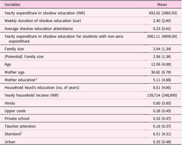
Table 1 summarizes the data. Children on an average spend INR 692 yearly on shadow education. Expenditure on shadow education constitutes significant part of the household expenditure, and often a typical middle-class household spends more money on shadow education than formal education. It can be quite normal then that there are enormous financial pressures on the parents in terms of investment in shadow education. For instance, shadow education constitutes around 5% of the annual household income in families where at least one child is attending shadow education. These families on average spend INR 3061 yearly on each child in shadow education. The average duration of shadow education is 2.40 hour per week.Footnote 10 In the data, nearly 23% of the students are taking shadow education. Compared to other related contexts, the figure looks conservative. For instance, 72% of 12th grade students take shadow education in Hong Kong (Zhan et al., Reference Zhan, Bray, Wang, Lykins and Kwo2013).Footnote 11
Summary statistics

Table 1. Long description
The table presents summary statistics on shadow education, including yearly expenditure, weekly duration, and average attendance. It highlights that children spend an average of INR 692 yearly on shadow education, with significant financial pressures on parents. Families with at least one child in shadow education spend around INR 3061 yearly per child, constituting about 5% of their annual household income. The average duration of shadow education is 2.40 hours per week, and approximately 23% of students participate in shadow education. The table includes data on family size, age, mother‘s age and education, household head’s education, yearly household income, religion, caste, school type, teacher attention, educational standard, and urban living status.
Notes: This Table reports means of the dependent variables and covariates. Standard errors are reported in parenthesis. Around 47% of the full sample constitute Girls. In calculating (potential) family size, I add observed family size with the number of additional children fathers want.
* Education: A bachelor’s degree is coded as 15, above bachelor’s as 16, and 1–12 grades are coded as 1–12 respectively.
† Grade of study: A bachelor’s degree is coded as 15, above bachelor’s as 16, and 1–12 grades are coded as 1–12 respectively.
The mean observed family size in our data is 2.94. If I add up the number of additional children their fathers further desire, the average (potential) family size increases to 2.96. The distribution of observed family size is as follows: 9.25% of children come from single-child families, 34.25% from two-child, 29.13% from three-child, and the rest from families with four or more children. The average age of a child is 12.06 years, and average current standard of study is 6.51 years. The sample is fairly representative. Around 80% of the children are Hindu, 28% of them belong to forward caste, and, 32% of the children are in the private schools. In the sample, the average maternal age is 36.62 years.
3. Empirical strategy
I want to estimate the (causal) effect of family size on shadow education expenditure. To do so, I consider the following specification: ${Y_{ij}} = \alpha + \beta {S_j} + \delta X + {\varepsilon _{ij}}$
where Y ij is the shadow education expenditure of child i in family j, Sj is the family size, and X is the vector of controls for cofounding characteristics, e.g., child age & its square, mother’s age and it’s square, and other background variables. Here, β is the coefficient of interest. Standard errors are adjusted for clustering at the primary sampling unit (PSU) level.Footnote 12
The primary challenge to estimate (1) is that quality and quantity are jointly determined by the parents. In other words, fertility is endogenous. Thus Sj may be related to the unobserved factors ϵij that affect shadow education expenditure: E (S j | ϵ ij ) ≠ 0. I use instrument variable to address this.
The empirical literature in fact tends to favor instrumental variables to alleviate such endogeneity concerns. For instance, Black et al. (Reference Black, Devereux and Salvanes2005) examine the QQ tradeoff in Norway using quasi-experimental variation due to twin birth; similarly, Angrist et al. (Reference Angrist, Lavy and Schlosser2010) use multiple instruments to test for QQ tradeoff in Israeli population. Specifically, the authors use twin and same-sex births in early birth orders as instrument for family size. Another paper by Rosenzweig and Zhang (Reference Rosenzweig and Zhang2009) tested the effect of twin instrument on twins themselves. In the Asian context, Lee (Reference Lee2008) instrument family size with first girl birth.
I use the occurrence of two back-to-back girl births as an instrumental variable for family size. For robustness, I also use two additional instruments: the first child being a girl and same-sex births in the first two parities.Footnote 13 My choice reflects strong gender-biased environment (Bose et al., Reference Bose, Arun and Arun2021), specifically elder son preference typically observed in the study context (Jayachandra & Pande, Reference Jayachandran and Pande2017). Thus, if the fertility goal is to have at least one son, a first-born daughter could induce parents to have one more child even if the desired family size is just one child, and similarly, if two subsequent children are girls, parents will try again for a son even if the fertility goal is just two. However, the birth of two consecutive daughters generates a substantially stronger and more predictable fertility response than the more generic same-sex composition. The two-girl instrument therefore maps directly into an economically meaningful and empirically validated stopping rule that affects subsequent parity progression and parental allocation decisions. In a handful of studies, gender-based instruments have been used (Lee, Reference Lee2008), and the instruments are argued to be well-suited in the Asian context (Lee, Reference Lee2008). On the other hand, same-sex is standard instrument in the QQ literature and has been used quite extensively.
I estimate the following 2SLS specification: ${Y_{ij}} = \beta {S_j} + \delta X + {\varepsilon _i}$ ${S_j} = \lambda Z + \alpha X + {\nu _j}$
where Z is the matrix of instruments and S is the family size. ϵ and ν are the error terms. X includes a constant. One caveat is that the linear IV model identifies linear relationship between family size and shadow education expenditures, and by doing so, it limits marginal effects of additional child to be the same across birth orders. To overcome this restriction, following previous literature I examine QQ tradeoff at the parities (Angrist et al., Reference Angrist, Lavy and Schlosser2010). Specifically, I begin by looking at the effects of second and higher parity births on first born children (I call 2+ sample). I further investigate the effects of third and higher parity births on firstborns, and, first and second born children (I call 3+ sample). This choice is motivated by the extensive literature documenting systematic differences in parental investments across birth orders. For example, Black et al. (Reference Black, Devereux and Salvanes2005) show that earlier-born children typically receive greater parental attention and educational investment relative to their later-born siblings. Subsequent work similarly finds that parents adjust investment strategies across siblings, often prioritizing earlier-born children. Focusing on first- and second-born children therefore allows the analysis to capture the effects of additional siblings on children who are most directly affected by resource reallocation when family size increases.
From an identification perspective, conditioning on early birth orders also provides a clearer interpretation of the quantity–quality (QQ) mechanism. When additional siblings arrive, parents must allocate household resources across a larger number of children, potentially reducing per-child investments such as tutoring expenditures. By focusing on first- and second-born children, the analysis isolates how parental behavior adjusts following exogenous fertility shocks while holding birth order relatively fixed. This approach is consistent with empirical strategies used in the QQ literature (e.g., Angrist et al., Reference Angrist, Lavy and Schlosser2010), where earlier-born children are often used as reference cases to study resource dilution.
4. IV estimates
I begin by providing descriptive evidence that family size and shadow education expenditures may be negatively related. Table A1 in the Appendix A shows the distribution of shadow education expenditures by family size. Shadow education expenditures monotonically decrease with family size. For instance, moving from single-child to two-child families, per-capita yearly shadow education expenditure reduces by INR 180 or by 16%. Furthermore, larger family size accompanies lower probability of shadow education attendance. Bigger families tend to have poorer socioeconomic backgrounds. I observe that both maternal education and household income monotonically drops with family size.
Next, I move on to the IV estimates. I begin by providing evidence on the relevance of the instruments. Fertility is the outcome of the interactions between desired family size and the desired sex ratio. Moreover, in our context, the sex-biased fertility-stopping behavior suggests that the probability of having subsequent children is not exogenous. The predictive power of the instruments lies on the strength of the elder son preference. Although the literature unambiguously indicates the existence of such elder son preference (Jayachandran & Pande, Reference Jayachandran and Pande2017; Arnold et al., Reference Arnold, Choe and Roy1998), I test a testable implication of elder son preference: families who have a daughter in early parity, would end up having a bigger family.
To assess the predictive strength of the instruments, linear probability models are estimated in which parity progression – the probability of having more than one child and more than two children – is the dependent variable. The principal explanatory variables are dummy indicators for two subsequent girls, first girl, and same-sex birth. The effect of having two subsequent girls is estimated in Table 2, which finds a larger effect: a 28.64 percentage points increase in the probability of having more than two children. As shown in Table A2, having a first girl increases the probability of having more than one child by 3.05 percentage points (column 1) and of having more than two children by 13.34 percentage points (column 2), both results statistically significant at the 1% level. Furthermore, column 2 also displays significant effects for the same-sex variable (13.94 percentage points), indicating robust associations with parity progression.
Parity progression

Table 2. Long description
The table presents data on the probability of having more than two children, with a specific focus on the effect of having two subsequent girls. It contains two rows and two columns. The first row is labeled ‘Dep variable’ and the second row is labeled ‘Two-girl’. The column headers are ‘Pr (n > 2)’ and the corresponding value is ‘0.2864*** (0.005)’. The table indicates that having two subsequent girls increases the probability of having more than two children by 28.64 percentage points.
Notes: Every column reports a separate linear regression. Standard errors reported in parenthesis are robust to within primary sampling unit (PSU) clustering. Estimations include controls for mother age and its square, maternal education, household income, household head’s education, and dummies for Hindu, forward caste and urban residence. Pr(n > 2) refer to the probabilities of having more than two children. ***p < 0.01; **p < 0.05; *p < 0.1.
Overall, evidence from Tables 2 and A2 supports that two subsequent girls, first girl, and same-sex birth are strong predictors of family size and spacing and are plausible instruments given their statistical significance and exogeneity.
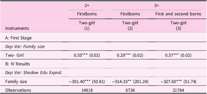
Table 3 displays parity-specific instrumental variable (IV) estimates using the two-girl instrument, with results divided into first-stage and second-stage estimates in Panels A and B, respectively. The first-stage results indicate strong positive effects, reflecting the prevalent elder son preference in the study context. As shown in Columns 1 and 2 for the sample of families with two or more children (2+ sample), having two subsequent girls increases average family size by 0.55 children, which is greater than the corresponding effects for first girl and same-sex birth (refer to Table A3). Notably, the impact of the two-girl instrument is largest in both the 2+ and 3+ samples. The second-stage estimates are consistently negative across both samples. For example, in families with 2 or more children, the 2SLS estimate for the effect of family size on yearly shadow education expenditure (using the two-girl instrument) is −391.40 INR (SE = 50.81). This indicates that an additional child, on average, reduces annual shadow education expenditures for firstborns by 391 INR. In comparison, instruments for first girl and same-sex birth yield estimates of −829.64 INR (SE = 167.83) and −134.77 INR (SE = 276.72), respectively (from Table A3, columns 1 and 2). The two-girl instrument offers somewhat greater precision. Similar patterns are observed in the sample with three or more children (3+ sample).
IV Estimates for shadow education expenditures

Table 3. Long description
The table presents instrumental variable estimates for shadow education expenditures, focusing on the impact of family size. It includes data for families with two or more children and three or more children, divided into firstborns and first and second borns. The table has four columns: the first column lists the instruments, the second and third columns show results for firstborns with two or more children, and the fourth column shows results for first and second borns with three or more children. The first stage results indicate a strong positive effect of having two girls on family size, with values of 0.55, 0.29, and 0.57 respectively. The second stage results show negative effects of family size on shadow education expenditures, with values of -391.40, -514.33, and -327.60 respectively. The table includes observations count for each scenario.
Notes: IV estimates. Standard errors reported in parenthesis are robust to within primary sampling unit (PSU) clustering. 2+ sample consists families with two or more children, and 3+ sample consists families with three and more children. I present estimates on the sub-sample with first born children in 2+ sample (column 1 and 2) and in 3+ sample (column 3 and 4). Additionally, column 4 and 5 present estimates on the sub-sample with first and second born children in 3+ sample. Panel A reports the first-stage estimates, and panel B reports IV estimates. All estimates include controls for child’s age and its square, current standard of study, mother age and its square, maternal education, household income, household head’s education, and dummies for private school and teacher attention at school, Hindu, forward caste and urban residence. ***p < 0.01; **p < 0.05; *p < 0.10.
Table A4 in the Appendix reports the estimates using standardized shadow education expenditures. I standardize the expenditure variable to have a mean of zero and a standard deviation of one. Based on the two-girl instrument, the estimated effects on standardized shadow education expenditures for first-born children are −0.15 SD and −0.19 SD in the 2+ and 3+ samples, respectively. For the sample including both first- and second-born children in the 3+ sample, the estimated effect is –0.13 SD. I observe similar negative effects when using the first-girl and same-sex instruments in the 2SLS estimates.
Table A5.1 in Appendix presents 2SLS estimates for the effect of family size on shadow education attendance. Consistent with the findings for shadow education expenditures, the estimated effects on attendance are uniformly negative and statistically significant when using the first girl and two-girl instruments. Specifically, an additional sibling reduces the probability of shadow education attendance for firstborns by 7 percentage points in families with two or more children and by 13 percentage points in families with three or more children (Table A5.1, columns 1 and 2). For both first- and second-born as girls in the 3+ sample, the likelihood of attending shadow education decreases by 7 percentage points (Table A5.1, column 3). Results for the first-girl instrument are similar: probability drops by 16-31 percentage points for firstborns and 8 percentage points for first and second born, respectively (Table A5.2). In contrast, the same-sex instrument does not yield statistically significant effects (Table A5.3).
Turning to the weekly duration of shadow education, Table A6 reports the IV estimates for weekly hours spent in private tutoring. The negative effects of family size persist across the 2SLS estimates. An additional child significantly reduces weekly shadow education hours for both first-born children and first- and second-born children. For example, using the two-girl instrument, the estimated effect for first-borns in the 2+ sample is −1.01 hours per week (Table A6, column 2) and −1.81 hours per week in the 3+ sample (Table A6, column 4), both statistically significant. The results remain qualitatively similar across alternative specifications and when using other instrumental variables.
4.1. Assessing the instruments
One must be careful in interpreting the IV estimates. It is important to consider what the effects mean. If there are heterogeneous effects, as it seems, each IV then generates its local effect. Essentially, the estimates tell us the effect of the specific group of additional children that we observe due to parental gender preference. Reassuringly however, I observe the QQ tradeoff across different set of instruments.
In this subsection I attempt to shed some lights on the instrument validity.Footnote 14 For causal interpretation, instruments should satisfy conditional independence assumption. This requires that the instrument is uncorrelated with background variables that affect shadow education expenditures. First-stage estimates provide some indication on the conditional independence of the instruments. Panels A and B of Table A7 in the Appendix A show that adding control for background variables have very little effects on the first-stage estimates, indicating the randomness of the instruments.
As a second test, to assess the “as good as random” assumption of the instruments, I estimate: $Z = \lambda X + \varphi$
where Z is the matrix of instruments as dependent variables and X denote the matrix of background variables that include a constant. I drop subscripts for notational simplicity. By estimating the above specification I find that apart from maternal characteristics most coefficients are statistically insignificant.Footnote 15 Better educated and older mothers are more likely to have a girl child and two subsequent girl children at the early parities, pointing at the importance of women’s intra-household status.Footnote 16 Nonetheless, even if maternal characteristics predict sex compositions, it is accounted for by the inclusion of a large set of maternal and family-specific socioeconomic controls in the estimation. However, if unobserved family characteristics predict sex compositions, it might be a problem. For instance, it is possible that women who have a first girl for instance, are positively selected on unobservable aspects related to women’s intra-household status. Then the IV estimates tend to have upward bias; essentially, in such case, IV estimates may generate upper bounds. In other words, the estimated effects could be an underestimate of the true QQ tradeoff.
To interpret the 2SLS estimands with multiple instruments as positively weighted average of local average treatment effects (LATE), the monotonicity condition must hold (Mogstad et al., Reference Mogstad, Torgovitsky and Walters2019).Footnote 17 The monotonicity condition requires monotonic effects of the instruments. To elucidate, in case of our binary instruments, family size induced by instruments (i.e., when Z = 1) should be at least as high as if the instruments take the value zero. While this is likely to hold, one testable implication that I test is that the first-stage estimates should be non-negative on any sub-population. When I estimate the first-stage estimates on few sub-populations, I find that the estimates are always positive and statistically significant (see Table A8 in the Appendix A).Footnote 18
Causal interpretation for heterogeneous IV models requires one further condition to hold – exclusion restriction. Together, under these conditions the estimates can be interpreted as average causal effects. Exclusion restriction requires that the instruments affect shadow education expenditures only through its impact on the family size. Strong son preference may induce parents to allocate resources away from girl child even from the first birth order. Put differently, instruments may affect shadow education expenditures for at least two reasons: an increase in the fertility and the sex composition of the children.
To make the issue more precise, it is informative to extend the baseline IV specification (2) into the following specification: $\quad\,\quad Y = \beta S + \delta X + \psi R + \varepsilon$ $S = \lambda Z + \alpha X + \nu$ $R = \phi Z + \pi X + \theta$
where R is the sex composition (proportion of girl child) in the household. The baseline IV estimates based on equation (2) are biased if Z correlates with R, and R affects Y holding S fixed conditional on X. The augmented IV model (3) may address this issue.Footnote 19
Table A9 in the Appendix A reports first-stage and IV estimates for (3). For the family size first stage, the coefficients have similar effects as before. For the sex composition first stage, first girl and two girls have positive effects. But, same-sex has negative effect. Looking at the IV estimates, family size effect on shadow education expenditures reduces but to me not appreciably compared to baseline IV estimates.Footnote 20 The Kleibergen-Paap Wald F statistics indicate that there is no evidence to suspect that the IV estimates are heavily affected by the problem of weak instruments.Footnote 21
The fact that instruments are related to some background variables, indicate that we should read results with caution. Considering these drawbacks, I further examine the QQ tradeoff by relaxing the validity assumption and estimate bounds on the IV estimates using imperfect IV procedure suggested by Nevo and Rosen (Reference Nevo and Rosen2012) and plausibly exogenous procedure suggested by Conley et al. (Reference Conley, Hansen and Rossi2012). In Appendix B, I show that Nevo and Rosen (Reference Nevo and Rosen2012) estimates produce negative bounds. In other words, the true IV estimates are inevitably negative, reassures the QQ tradeoff. In Appendix C, I estimate bounds suggested by Conley et al. (Reference Conley, Hansen and Rossi2012) on the premise that instruments are plausibly if not strictly exogenous. Reassuringly again, the Conley et al. (Reference Conley, Hansen and Rossi2012) approach produces negative bounds.
4.2. Potential selection bias
Because a large share of children does not participate in shadow education, the sample of tutoring expenditures may be subject to non-random selection. To address this concern, I implement an inverse probability weighting (IPW) approach to correct for potential selection bias. When the dependent variable is observed only for a selected subsample, IPW provides a standard method for mitigating selection issues by reweighting observations based on their probability of inclusion in the sample.
Specifically, I first estimate the probability that a child participates in shadow education using a probit model. The predicted probabilities from this model are then used to construct inverse probability weights, which adjust the sample so that observations with a lower likelihood of selection receive greater weight. This procedure helps correct for potential distortions arising from the non-random participation in shadow education.
I then apply these inverse probability weights as sample weights in the baseline fixed-effects regressions. The results from the IPW-weighted estimations are reported in Table A10 in the Appendix. The estimated coefficients remain both qualitatively and quantitatively similar to the baseline results, suggesting that the main findings are robust to potential selection bias arising from non-participation in shadow education.
5. Heterogeneity analysis by caste, residence, and schooling type
To better interpret the instrumental variable estimates, the heterogeneous impact of family size on shadow education expenditures is assessed by estimating the 2SLS model across key subgroups defined by caste, residence, and schooling type. The sample is split by forward and backward caste, rural and urban residence, and private versus public schooling. Although splitting by neighborhood and schooling may introduce some endogeneity, these group distinctions are highly relevant to the Indian context.
Backward caste families, historically economically and educationally disadvantaged, display a larger average family size (3.02 children) compared to forward caste families (2.73 children) and earn substantially less annual income. Rural populations are generally poorer and have higher family size than urban populations, with an average family size of 3.04 compared to 2.75, respectively. Moreover, children in public schools tend to spend less on shadow education than those in private schools. These underlying differences warrant subgroup-specific estimates.
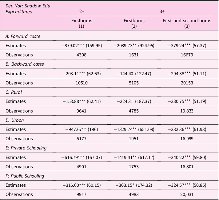
Table 4 presents IV estimates for each subgroup using the two-girl instrument. Across all panels, the estimates are negative, indicating that an increase in family size reduces shadow education expenditure. The effect is largest for forward caste families, urban residents, and private school students, groups that overlap in socioeconomic status and educational aspirations. For example, the effect for forward castes on firstborns in the 2+ sample is −879.02 INR (p < 0.01), while for backward caste it is −203.11 INR (p < 0.01). Urban families experience a reduction of −947.67 INR (p < 0.05), contrasted with −158.88 INR (p < 0.01) for rural families. Private schooling shows a drop of −616.79 INR (p < 0.01), whereas public schooling’s reduction is −316.60 INR (p < 0.01). These differences are even more pronounced for families with three or more children and for estimates on the first and second born.Footnote 22
Heterogeneity Analysis with two girls as an instrument

Table 4. Long description
The table presents IV estimates for shadow education expenditures across various subgroups using the two-girl instrument. It includes data for forward caste, backward caste, rural, urban, private schooling, and public schooling categories. The table has six rows for each subgroup and three columns for different family structures: firstborns with two or more children, firstborns with three or more children, and first and second borns with three or more children. Each cell contains estimates and observations. For forward caste families, the estimates range from negative 879.02 INR to negative 2089.73 INR, indicating a significant reduction in shadow education expenditure with an increase in family size. Backward caste families show estimates from negative 203.11 INR to negative 294.38 INR. Urban families experience a reduction of negative 947.67 INR to negative 1329.74 INR, while rural families see a decrease from negative 158.88 INR to negative 330.75 INR. Private schooling estimates range from negative 616.79 INR to negative 1419.41 INR, and public schooling estimates range from negative 316.60 INR to negative 324.57 INR. The data suggests that the effect is largest for forward caste families, urban residents, and private school students, groups that overlap in socioeconomic status and educational aspirations.
Notes: IV estimates with two girls as the instrument. Standard errors reported in parenthesis are robust to within primary sampling unit (PSU) clustering. All estimates include controls for child’s age and its square, current standard of study, mother age and its square, maternal education, household income, household head’s education, and dummies for private school and teacher attention at school, Hindu, forward caste and urban residence.
***p < 0.01; **p < 0.05; *p < 0.10.
These substantial caste, residence, and schooling divides are particularly interesting. In spite of being wealthier and better educated, larger QQ effects in forward caste and urban families are surprising. One possible explanation is that forward caste group and more so those in the urban areas have incorporated the contemporary norm of keeping the family size small and invest on children heavily. On the other hand, backward caste group may arguably have more liberal outlook to the family size. In addition, shadow education expenditure is found to be driven by the parental concern of children’s future status in society (Yum et al., unpublished). Related, in the Indian context, urban forward caste group are likely to have more concern over their children’s future status.
Importantly, this pattern echoes macro-historical evidence that the quantity–quality trade-off tends to emerge first among socioeconomically advantaged groups. Unified Growth Theory (Galor & Moav, Reference Galor and Moav2002; Galor, Reference Galor2011) posits that elites with high returns to human capital are the earliest to substitute child quality for quantity, initiating the transition away from Malthusian dynamics. Recent historical work by Baudin and de la Croix (Reference Baudin and De la Croix2025) similarly shows that in pre-industrial Europe, scholars and other high-status groups internalized the QQ trade-off long before the wider population. The stronger trade-offs observed among forward-caste and urban households in India today may therefore represent a contemporary analogue of this pattern: groups facing the highest returns to human capital investment are the first to exhibit Beckerian fertility–investment behavior, while others could remain closer to Malthusian norms.
6. Conclusion
This paper has revisited the child quantity–quality tradeoff by focusing on parental expenditures on shadow education in India. Using instruments derived from son preference, I identify a robust negative effect of additional siblings on per-child tutoring expenditures. Each additional child reduces shadow education spending by 0.13–0.19 standard deviations, with stronger effects in advantaged and urban households.
These findings make a contribution by shifting attention from downstream outcomes to direct monetary allocations within households. Previous studies have often been forced to infer parental resource allocation indirectly through educational attainment or labor-market success. By focusing on expenditures in shadow education, this study provides sharper evidence of how fertility directly shapes parental investments in child quality. In developing-country contexts where private tutoring constitutes a major component of household educational spending, shadow education expenditures provide a particularly informative lens through which to study parental investment behavior and the quantity–quality tradeoff.
Family planning is one of the fiercely debated issues in contemporary India. Most Indian states either have some policies to control fertility or planning for one such.Footnote 23 The underlying motivation is the QQ tradeoff. High fertility is often argued to be a major obstacle to human capital accumulation. In modern economies, the quality of human capital, rather than its quantity is the backbone of economic growth and development. The QQ tradeoff thesis conditions such child quality on child quantity. The conclusion of the most recent studies of no family size effect indicates that we should not be worried about the family size. By contrast, I contest recent literature by showing a QQ tradeoff. Thus, my results may strengthen the case of family planning policies. At the macro level, the results align with development theories and family planning perspectives that position the QQ trade-off at the core of growth dynamics. The evidence that lower fertility increases per-child educational investment provides a micro-foundation for the macro rationale underlying family planning initiatives, namely that fertility decline can accelerate human capital accumulation and, in turn, long-run economic development. However, there is need to be cautious. The study context also features strong son preference. An uninformed family planning policy without due considerations to the girl disadvantages can be disastrous. Specifically, in a strong family policy regime, any unintended girl child may suffer more with reduced parental resources. An exogenous incentive to reduce family size may strengthen son preference and results in more sex-biased population.Footnote 24 In sum, the evidence suggests an integrated policy framework which should aim to reduce family size together with incentivizing parents to have girl child, and invest on them equally.
Supplementary material
To view supplementary material for this article, please visit https://doi.org/10.1017/dem.2026.10024.
Acknowledgements
I thank Arjun Bedi, Mark Bray, and Matthias Rieger for their helpful comments and suggestions. I thank Editor David de la Croix and the anonymous referee for their helpful comments and suggestions. I thank Adityava Majumder and Anisha Shukla for research assistance. I declare that I have no relevant or material financial interests that relate to the research described in this paper.



 Open access

