


1 Introduction
The Gieseker moduli space ${\mathfrak M}_{1,3}$
of canonical models of surfaces of general type with
${\mathfrak M}_{1,3}$
of canonical models of surfaces of general type with $K_X^2 =1$
and
$K_X^2 =1$
and $\chi (X) = 3$
is a rational variety of dimension 28 and it was classically known that the surfaces it parametrises are hypersurfaces of degree 10 contained in the smooth locus of
$\chi (X) = 3$
is a rational variety of dimension 28 and it was classically known that the surfaces it parametrises are hypersurfaces of degree 10 contained in the smooth locus of ${\mathbb P}(1,1,2,5)$
. More geometrically speaking, the bicanonical map realises these surfaces as double covers of the quadric cone in
${\mathbb P}(1,1,2,5)$
. More geometrically speaking, the bicanonical map realises these surfaces as double covers of the quadric cone in ${\mathbb P}^3$
branched over the vertex and a sufficiently general quintic section.
${\mathbb P}^3$
branched over the vertex and a sufficiently general quintic section.
Nowadays, the Gieseker moduli space ${\mathfrak M}_{a,b}$
is known to admit a modular compactification
${\mathfrak M}_{a,b}$
is known to admit a modular compactification $\overline {{\mathfrak M}}_{a,b}$
, the moduli space of stable surfaces with
$\overline {{\mathfrak M}}_{a,b}$
, the moduli space of stable surfaces with $K_X^2 =a$
and
$K_X^2 =a$
and $\chi (X) = b$
, sometimes called KSBA-moduli space after Kollár, Shepherd-Barron and Alexeev (compare [Reference KollárKol23]). For brevity we call the surfaces parametrised by
$\chi (X) = b$
, sometimes called KSBA-moduli space after Kollár, Shepherd-Barron and Alexeev (compare [Reference KollárKol23]). For brevity we call the surfaces parametrised by $\overline {{\mathfrak M}}_{1,3}$
stable I-surfaces (see Definition 2.2 for a precise definition).
$\overline {{\mathfrak M}}_{1,3}$
stable I-surfaces (see Definition 2.2 for a precise definition).
Our detailed understanding of the Gieseker moduli space, or classical component, and the small values of the invariants make $\overline {{\mathfrak M}}_{1,3}$
into a fertile testing ground to explore stable surfaces and their moduli.
$\overline {{\mathfrak M}}_{1,3}$
into a fertile testing ground to explore stable surfaces and their moduli.
So far a full picture seems out of reach, and the current approaches aim for classification under some extra conditions on the singularities. The first result in this direction was the extension of the classical description to Gorenstein stable I-surfaces [Reference Franciosi, Pardini and RollenskeFPR17], which was refined and explored further in [Reference Coughlan, Franciosi, Pardini and RollenskeCFPR22] from a Hodge theoretic perspective. In [Reference Franciosi, Pardini, Rana and RollenskeFPRR22, Reference Coughlan, Franciosi, Pardini, Rana and RollenskeCFP+23] we explored surfaces with few T-singularities, finding several divisors and an additional component. Meanwhile in [Reference Gallardo, Pearlstein, Schaffler and ZhangGPSZ24] Gallardo, Pearlstein, Schaffler and Zhang found eight more divisors by considering the stable replacement of Gorenstein degenerations with an exceptional unimodal singularity; in [Reference Rollenske and TorresRT24] it was shown that there are not more divisors of this kind.
In the present paper we completely classify 2-Gorenstein stable I-surfaces, that is, those with $2K_X$
Cartier, dividing them into four types:
$2K_X$
Cartier, dividing them into four types:
Theorem 1.1. Let X be a 2-Gorenstein stable I-surface. Then X is one of the following:
-
type A Semi-log-canonical hypersurfaces in ${\mathbb P}(1,1,2,5)$
not passing through the point
$(0:0:0:1)$
. This includes all Gorenstein stable I-surfaces and the divisor whose general element is a surface with one singularity of type
$\frac 14(1,1)$
.
${\mathbb P}(1,1,2,5)$
not passing through the point
$(0:0:0:1)$
. This includes all Gorenstein stable I-surfaces and the divisor whose general element is a surface with one singularity of type
$\frac 14(1,1)$
. -
type B These are reducible surfaces
$X = X_1 \cup X_2$
, where
$X_1$
is a singular Enriques surface and
$X_2$
is a singular K3 surface. They form a family of dimension
$27$
in the closure of the Gieseker component, thus are smoothable, but no longer complete intersections. -
type DD These are reducible complete intersections of bidegree
$(2,10)$
in weighted projective space
${\mathbb P}(1,1,2,2,5)$
and the bicanonical map realises them as double covers of the union of two planes. Each component is a singular K3 surface and they form a subset of codimension two in the closure of the Gieseker component. -
type DE These are reducible surfaces
$X = X_1 \cup X_2$
, where both
$X_i$
are singular K3 surfaces of a special kind. They form a 30-dimensional family and none of them is smoothable, that is, they form a new irreducible component. Their canonical ring is quite complicated.


We give an overview of the known strata in $\overline {{\mathfrak M}}_{1,3}$
in Table 1, including dimension of the stratum, index of the general surface and a reference to precise information and proofs.
$\overline {{\mathfrak M}}_{1,3}$
in Table 1, including dimension of the stratum, index of the general surface and a reference to precise information and proofs.
Known irreducible strata in the moduli space $\overline {\mathfrak M}_{1,3}$
of stable I-surfaces.
$\overline {\mathfrak M}_{1,3}$
of stable I-surfaces.

Our current knowledge of the locus of 2-Gorenstein stable I-surfaces in relation to the rest of $\overline {{\mathfrak M}}_{1,3}$
is shown in Figure 1. We have not studied possible degenerations of the surfaces in the previously unknown component
$\overline {{\mathfrak M}}_{1,3}$
is shown in Figure 1. We have not studied possible degenerations of the surfaces in the previously unknown component ${\mathfrak M}^{DE}$
and we would not dare to speculate if it is a connected component without further evidence.
${\mathfrak M}^{DE}$
and we would not dare to speculate if it is a connected component without further evidence.
Known strata in $\overline {{\mathfrak M}}_{1,3}$
(compare Table 1 for notation).
$\overline {{\mathfrak M}}_{1,3}$
(compare Table 1 for notation).

Outline of the paper and proof of Theorem 1.1
Let X be a 2-Gorenstein stable I-surface as defined in Definition 2.2. Then we show in Proposition 3.3 that the general section of $\omega _X$
does not vanish on any component and thus defines a canonical curve C.
$\omega _X$
does not vanish on any component and thus defines a canonical curve C.
If C can be chosen reduced, then we use the hyperplane section principle [Reference ReidRei90] and our work on generalised Gorenstein spin structures on reduced curves of genus two [Reference Coughlan, Franciosi, Pardini and RollenskeCFPR23] (summarised in Theorem 3.8) to compute the canonical ring. This gives the surfaces of type A and type B, classified in Sections 4 and 5.
We were unable to argue along the same lines when the general canonical curve is nonreduced. However, in this case the surface is reducible and we succeed in giving a geometric description of the components and the possible glueings, resulting in two cases (Lemma 6.3).
Type DD is identified in Section 7 with a smoothable example already considered in [Reference Franciosi, Pardini and RollenskeFPR17]. Type DE is shown to give a new irreducible component in Section 8; its canonical ring is computed a posteriori from the geometric description.
2 Notation and preliminary results
2.1 Set-up
We work with schemes of finite type over the complex numbers.
Given a sheaf ${\mathcal F}$
on a scheme X, we denote by
${\mathcal F}$
on a scheme X, we denote by ![]() its dual and by
its dual and by ${\mathcal F}^{[m]}$
the m-th reflexive power, i.e., the double dual of
${\mathcal F}^{[m]}$
the m-th reflexive power, i.e., the double dual of ${\mathcal F}^{\operatorname {\mathrm {\otimes }} m}$
.
${\mathcal F}^{\operatorname {\mathrm {\otimes }} m}$
.
A curve C is a Cohen–Macaulay projective scheme of pure dimension 1 (possibly nonreduced or reducible). It has a dualising sheaf $\omega _C$
and we denote by
$\omega _C$
and we denote by $p_a(C)$
the arithmetic genus of C, that is,
$p_a(C)$
the arithmetic genus of C, that is, ![]() . The curve C is Gorenstein if
. The curve C is Gorenstein if $\omega _C$
is invertible; if this is the case
$\omega _C$
is invertible; if this is the case $K_C$
denotes a canonical divisor such that
$K_C$
denotes a canonical divisor such that ![]() .
.
Our standard reference for stable surfaces is [Reference KollárKol13]. A stable surface X has semi-log-canonical singularities and ample canonical divisor. In particular, it is by definition Cohen–Macaulay and Gorenstein in codimension one, so the canonical sheaf $\omega _X$
exists and is reflexive. We call
$\omega _X$
exists and is reflexive. We call $X m$
-Gorenstein if the m-th reflexive power of the canonical sheaf
$X m$
-Gorenstein if the m-th reflexive power of the canonical sheaf $\omega _X^{[m]}$
is invertible. A canonical divisor is a Weil divisor
$\omega _X^{[m]}$
is invertible. A canonical divisor is a Weil divisor $K_X$
such that
$K_X$
such that ![]() . We use the notations
. We use the notations ![]() ,
, $p_g(X) = h^0(X, \omega _X)$
and
$p_g(X) = h^0(X, \omega _X)$
and ![]() .
.
If X is a non-normal stable surface, then we denote by $\pi \colon \bar X \to X$
the normalisation of X and by
$\pi \colon \bar X \to X$
the normalisation of X and by $D\subset X $
and
$D\subset X $
and $ \bar D\subset \bar X$
the curves defined by the conductor ideal
$ \bar D\subset \bar X$
the curves defined by the conductor ideal ![]() . The invariants are related by
. The invariants are related by $K_X^2 = (K_{\bar X}+\bar D)^2$
and
$K_X^2 = (K_{\bar X}+\bar D)^2$
and $\chi (X) = \chi ({\bar X})+\chi (D)-\chi ({\bar D})$
(see also [Reference Franciosi, Pardini and RollenskeFPR15, Prop. 3.3]).
$\chi (X) = \chi ({\bar X})+\chi (D)-\chi ({\bar D})$
(see also [Reference Franciosi, Pardini and RollenskeFPR15, Prop. 3.3]).
The map $\pi \colon \bar D \to D$
on the conductor divisors is generically a double cover and thus induces a rational involution on
$\pi \colon \bar D \to D$
on the conductor divisors is generically a double cover and thus induces a rational involution on $\bar D$
. Normalising the conductor loci we get an honest involution
$\bar D$
. Normalising the conductor loci we get an honest involution $\tau \colon \bar D^\nu \to \bar D^\nu $
such that
$\tau \colon \bar D^\nu \to \bar D^\nu $
such that $D^\nu = \bar D^\nu /\tau $
and such that the different
$D^\nu = \bar D^\nu /\tau $
and such that the different ${\mathsf {Diff}}_{\bar D^\nu }(0)$
is
${\mathsf {Diff}}_{\bar D^\nu }(0)$
is $\tau $
-invariant, which fits in the following pushout diagram:
$\tau $
-invariant, which fits in the following pushout diagram:

By Kollár’s glueing construction [Reference KollárKol13, Thm. 5.13], the surface X can be reconstructed uniquely from the triple $(\bar X, \bar D, \tau )$
.
$(\bar X, \bar D, \tau )$
.
2.2 I-surfaces
Our main interest stems from the Gieseker moduli space ${\mathfrak M}_{1,3}$
and its closure in the moduli space of stable surfaces.
${\mathfrak M}_{1,3}$
and its closure in the moduli space of stable surfaces.
For canonical or just Gorenstein stable surfaces X with fixed $K_X^2$
and
$K_X^2$
and $\chi (X)$
the Riemann–Roch formula and Kodaira vanishing determine all higher plurigenera as
$\chi (X)$
the Riemann–Roch formula and Kodaira vanishing determine all higher plurigenera as $P_m(X) = \chi (X) + \frac 12 m(m-1)K_X^2$
for
$P_m(X) = \chi (X) + \frac 12 m(m-1)K_X^2$
for $m\geq 2$
. Together with the geometric genus
$m\geq 2$
. Together with the geometric genus $p_g$
or equivalently the irregularity q this determines the Hilbert function of the canonical ring
$p_g$
or equivalently the irregularity q this determines the Hilbert function of the canonical ring $R(X, K_X)$
.
$R(X, K_X)$
.
By Noether’s inequality or [Reference Franciosi, Pardini and RollenskeFPR17] a Gorenstein stable surface with $K_X^2=1$
and
$K_X^2=1$
and $\chi (X) = 3$
satisfies
$\chi (X) = 3$
satisfies $q(X) =0$
and thus has Hilbert seriesFootnote
1
$q(X) =0$
and thus has Hilbert seriesFootnote
1
 $$ \begin{align} \frac{1-t^{10}}{(1-t)^2(1-t^2)(1-t^5)}. \end{align} $$
We will show below in Proposition 3.3 that this continues to hold if X is only $2$
-Gorenstein.
$2$
-Gorenstein.
If the Cartier index of X is larger, this is no longer true:
Example 2.1. Let $X=X_9\subset {\mathbb P}(1,1,3,3)$
a general hypersurface of degree
$X=X_9\subset {\mathbb P}(1,1,3,3)$
a general hypersurface of degree $9$
. Then X has three singularities of type
$9$
. Then X has three singularities of type $\frac 13 (1,1)$
and
$\frac 13 (1,1)$
and ![]() . Thus
. Thus $3K_X$
is Cartier and ample, so X is stable. The invariants are
$3K_X$
is Cartier and ample, so X is stable. The invariants are $K_X^2 = 1$
,
$K_X^2 = 1$
, $\chi (X) = 3$
with
$\chi (X) = 3$
with $p_g(X) = 2$
. However,
$p_g(X) = 2$
. However, ![]() .
.
This example and more general instances of this phenomenon were considered in [Reference RollenskeRol23].
To exclude such pathological examples that are unrelated to the study of canonical surfaces, we specify the Hilbert series in our definition.
Definition 2.2. A stable I-surface is a stable surface with $K_X^2=1$
,
$K_X^2=1$
, $\chi (X) = 3$
and Hilbert series of the canonical ring as in (2.2), in particular
$\chi (X) = 3$
and Hilbert series of the canonical ring as in (2.2), in particular $p_g(X) = 2$
and
$p_g(X) = 2$
and $q(X)=0$
.
$q(X)=0$
.
We denote the moduli space of stable I-surfaces by $\overline {\mathfrak M}_{1,3}$
, the closure of the Gieseker component inside it by
$\overline {\mathfrak M}_{1,3}$
, the closure of the Gieseker component inside it by $\overline {\mathfrak M}_{1,3}^{\text {class}}$
.
$\overline {\mathfrak M}_{1,3}^{\text {class}}$
.
3 Existence of canonical curves and consequences
If X is a stable surface, we say that X contains a canonical curve if there is a section $x_0\in H^0(X, \omega _X)$
which is nonzero at each generic point. In the irreducible case this just means that
$x_0\in H^0(X, \omega _X)$
which is nonzero at each generic point. In the irreducible case this just means that $x_0\neq 0$
, in general it can happen that a section vanishes identically on some but not every component.
$x_0\neq 0$
, in general it can happen that a section vanishes identically on some but not every component.
Example 3.1. Let C be a smooth plane quartic, $X_1=S^2C$
and
$X_1=S^2C$
and $D_1$
a coordinate curve. We have
$D_1$
a coordinate curve. We have $p_g(X_1) = q(X_1) = 3$
and
$p_g(X_1) = q(X_1) = 3$
and $K_{X_1}^2 = 6$
(see [Reference Hacon and PardiniHP02, Example 1]). Since
$K_{X_1}^2 = 6$
(see [Reference Hacon and PardiniHP02, Example 1]). Since $D_1$
is ample, the Riemann–Roch formula gives
$D_1$
is ample, the Riemann–Roch formula gives $h^0(K+D_1)=3=h^0(K)$
, so that
$h^0(K+D_1)=3=h^0(K)$
, so that $D_1$
is in the fixed part of
$D_1$
is in the fixed part of $|K+D_1|$
.
$|K+D_1|$
.
Now take $(X_2, D_2)=({\mathbb P}^2, C)$
and glue
$(X_2, D_2)=({\mathbb P}^2, C)$
and glue $D_1\cong C \cong D_2$
to get a stable surface X, which consists of the two components intersecting with normal crossings in the curve C. One can check that
$D_1\cong C \cong D_2$
to get a stable surface X, which consists of the two components intersecting with normal crossings in the curve C. One can check that $K_X^2 = 13$
,
$K_X^2 = 13$
, $p_g(X) = 3$
and
$p_g(X) = 3$
and $q(X) = 0$
.
$q(X) = 0$
.
By the above, all canonical sections vanish on the intersection curve, because their pullback to the normalisation vanishes on $D_1$
, thus they vanish identically on the component
$D_1$
, thus they vanish identically on the component $X_2$
and there is no canonical curve.
$X_2$
and there is no canonical curve.
3.1 Existence of canonical curves
In this section we prove the existence of canonical curves on any $2$
-Gorenstein stable I-surface. We start with slightly weaker hypotheses, which we then prove to imply that we have a stable I-surface.
$2$
-Gorenstein stable I-surface. We start with slightly weaker hypotheses, which we then prove to imply that we have a stable I-surface.
Lemma 3.2. Let X be a reducible 2-Gorenstein stable surface with $K_X^2 = 1$
and
$K_X^2 = 1$
and $\chi (X) = 3$
. Then:
$\chi (X) = 3$
. Then:
-
1. the normalisation
$(\bar X,\bar D)$
of
$\bar X$
is equal to
$(\bar X_1, \bar D_1)\sqcup (\bar X_2, \bar D_2)$
, with
$\bar X_i$
irreducible and
$\bar D_i>0$
,
$i=1,2$
; -
2. for
$i=1,2$
the divisor
$K_{\bar X_i}+\bar D_i$
is 2-Cartier and ample with
$(K_{\bar X_i}+\bar D_i )^2=\frac 12$
.


Proof. Let $\pi \colon \bar X = \bigsqcup _{i=1}^r\bar X_i \to X$
be the normalisation. Since
$\pi \colon \bar X = \bigsqcup _{i=1}^r\bar X_i \to X$
be the normalisation. Since $2K_X$
is an ample Cartier divisor, its pullback
$2K_X$
is an ample Cartier divisor, its pullback $\pi ^* 2K_X|_{\bar X_i} = 2( K_{\bar X_i} + \bar D_i)$
is an ample Cartier divisor as well, and
$\pi ^* 2K_X|_{\bar X_i} = 2( K_{\bar X_i} + \bar D_i)$
is an ample Cartier divisor as well, and
 $$\begin{align*}2 = 2K_X^2 = \sum_{i=1}^r \left(2(K_{\bar X_i} + \bar D_i)\right)(K_{\bar X_i} + \bar D_i) .\end{align*}$$
Because the intersection of an ample Cartier divisor with a Weil divisor is a positive integer and because by assumption we have more than one component, we get $r = 2$
and
$r = 2$
and $(K_{\bar X_i} + \bar D_i)^2= \frac 12$
. The divisors
$(K_{\bar X_i} + \bar D_i)^2= \frac 12$
. The divisors $ \bar D_i$
cannot be zero, because they contain the preimage of the intersection of the two components, which is a curve because X is
$ \bar D_i$
cannot be zero, because they contain the preimage of the intersection of the two components, which is a curve because X is $S_2$
and connected.
$S_2$
and connected.
If X is a reducible 2-Gorenstein stable surface with $K_X^2 = 1$
and
$K_X^2 = 1$
and $\chi (X) = 3$
and normalisation
$\chi (X) = 3$
and normalisation $(\bar X_1, \bar D_1)\sqcup (\bar X_2, \bar D_2)$
, we write
$(\bar X_1, \bar D_1)\sqcup (\bar X_2, \bar D_2)$
, we write $\bar D_i= \bar Z_i+ \bar \Gamma _i$
, where
$\bar D_i= \bar Z_i+ \bar \Gamma _i$
, where $\bar \Gamma _1$
is glued to
$\bar \Gamma _1$
is glued to $ \bar \Gamma _2$
by
$ \bar \Gamma _2$
by $\pi $
, while
$\pi $
, while $ \bar Z_i$
is glued to itself for
$ \bar Z_i$
is glued to itself for $i=1,2$
. Note that
$i=1,2$
. Note that $ \bar \Gamma _i>0$
since X is connected and
$ \bar \Gamma _i>0$
since X is connected and $S_2$
, while
$S_2$
, while $\bar Z_i$
may be zero.
$\bar Z_i$
may be zero.
With this notation in place we can state the main result of this section:
Proposition 3.3. Let X be a 2-Gorenstein stable surface with $K_X^2 = 1$
and
$K_X^2 = 1$
and $\chi (X) = 3$
. Then:
$\chi (X) = 3$
. Then:
-
1. the zero locus of a general section of
$H^0(K_X)$
is one-dimensional; -
2.
$q(X)=0$
and X is a stable I-surface; -
3. all canonical curves are nonreduced if and only if
$X=X_1\cup X_2$
is reducible and
$K_{\bar X_i}+\bar Z_i=0$
for
$i=1,2$
. In this case, every canonical curve is supported on
$X_1\cap X_2$
.


Before proving Proposition 3.3 we give some auxiliary results.
Lemma 3.4. Let Y be a smooth projective surface and let M be a nef line bundle. If $M^2=2$
, then
$M^2=2$
, then $h^0(M)\le 4$
.
$h^0(M)\le 4$
.
Proof. We can of course assume that $r:=h^0(M)-1\ge 1$
, otherwise the statement is empty. Write
$r:=h^0(M)-1\ge 1$
, otherwise the statement is empty. Write $|M|=Z+|D|$
, where Z is the fixed part and D the moving part, denote by
$|M|=Z+|D|$
, where Z is the fixed part and D the moving part, denote by $h\colon X\to {\mathbb P}^r$
the map defined by
$h\colon X\to {\mathbb P}^r$
the map defined by $|D|$
and let d be the degree of the image
$|D|$
and let d be the degree of the image $\Sigma $
of h. Assume first that
$\Sigma $
of h. Assume first that $\Sigma $
is a surface: then since M and D are nef we have
$\Sigma $
is a surface: then since M and D are nef we have $2=M^2\ge MD\ge D^2\ge d\ge r-1$
, hence
$2=M^2\ge MD\ge D^2\ge d\ge r-1$
, hence $r\leq 3$
. If instead
$r\leq 3$
. If instead $\Sigma $
is a curve, then D is numerically equivalent to
$\Sigma $
is a curve, then D is numerically equivalent to $dG$
, where G is irreducible and
$dG$
, where G is irreducible and $2=M^2\ge MD=dMG\ge d\ge r$
, so
$2=M^2\ge MD=dMG\ge d\ge r$
, so $r\le 2$
in this case.
$r\le 2$
in this case.
If $X=X_1\cup X_2$
is a reducible stable 2-Gorenstein stable surface with
$X=X_1\cup X_2$
is a reducible stable 2-Gorenstein stable surface with $K_X^2 = 1$
and
$K_X^2 = 1$
and $\chi (X) = 3$
, then we denote by
$\chi (X) = 3$
, then we denote by
 $$\begin{align*}\rho=(\rho_1, \rho_2) \colon H^0(K_X)\to H^0(K_{\bar X_1}+\bar D_1)\oplus H^0(K_{\bar X_2}+\bar D_2) \end{align*}$$
the pullback map.
Lemma 3.5. In the above set-up and notation, assume that $\rho _1$
is not injective: then
$\rho _1$
is not injective: then $\dim \ker \rho _1=1$
and
$\dim \ker \rho _1=1$
and $K_{\bar X_2}+ \bar Z_2=0$
.
$K_{\bar X_2}+ \bar Z_2=0$
.
Proof. Set $L_i:=2(K_{\bar X_i}+\bar D_i)$
for
$L_i:=2(K_{\bar X_i}+\bar D_i)$
for $i=1,2$
. Recall that by assumption
$i=1,2$
. Recall that by assumption $L_i$
is an ample line bundle with
$L_i$
is an ample line bundle with $L_i ^2=2$
. Consider
$L_i ^2=2$
. Consider $0\ne \sigma \in \ker \rho _1$
: since
$0\ne \sigma \in \ker \rho _1$
: since $\rho $
is injective,
$\rho $
is injective, $\rho _2(\sigma )$
is a nonzero section of
$\rho _2(\sigma )$
is a nonzero section of $K_{\bar X_2}+\bar D_2$
that vanishes on
$K_{\bar X_2}+\bar D_2$
that vanishes on $\bar \Gamma _2$
, hence
$\bar \Gamma _2$
, hence $K_{\bar X_2}+ \bar Z_2\ge 0$
. Since
$K_{\bar X_2}+ \bar Z_2\ge 0$
. Since $L_2$
is ample,
$L_2$
is ample, $1=L_2(K_{\bar X_2}+\bar D_2)=L_2(K_{\bar X_2}+ \bar Z_2)+L _2 \bar \Gamma _2$
and
$1=L_2(K_{\bar X_2}+\bar D_2)=L_2(K_{\bar X_2}+ \bar Z_2)+L _2 \bar \Gamma _2$
and $\bar \Gamma _2>0$
give
$\bar \Gamma _2>0$
give $L_2 \bar \Gamma _2=1$
,
$L_2 \bar \Gamma _2=1$
, $L_2(K_{\bar X_2}+ \bar Z_2)=0$
, therefore
$L_2(K_{\bar X_2}+ \bar Z_2)=0$
, therefore $K_{\bar X_2}+ \bar Z_2=0$
and
$K_{\bar X_2}+ \bar Z_2=0$
and $ \bar \Gamma _2$
is irreducible. Note that
$ \bar \Gamma _2$
is irreducible. Note that $\bar \Gamma _2$
is the divisor of
$\bar \Gamma _2$
is the divisor of $\rho _2(\sigma )$
. If
$\rho _2(\sigma )$
. If $0\ne \tau $
is another element of
$0\ne \tau $
is another element of $\ker \rho _1$
, then the divisor of
$\ker \rho _1$
, then the divisor of $\rho _2(\tau )$
is also equal to
$\rho _2(\tau )$
is also equal to $\bar \Gamma _2$
and therefore,
$\bar \Gamma _2$
and therefore, $\rho _2(\tau )$
and
$\rho _2(\tau )$
and $\rho _2(\sigma )$
are linearly dependent. Since
$\rho _2(\sigma )$
are linearly dependent. Since $\rho $
is injective, it follows that
$\rho $
is injective, it follows that $\ker \rho _1$
has dimension 1.
$\ker \rho _1$
has dimension 1.
Proof of Proposition 3.3.
-
1. Assume for contradiction that all sections of
$K_X$
have a two-dimensional zero locus. Then
$X=X_1\cup X_2$
is reducible and we may assume that all sections of
$K_X$
vanish on
$X_1$
. By Lemma 3.5 we get
$p_g(X)\le 1$
, contradicting
$\chi (X)=3$
. -
2. Assume for contradiction
$q(X)>0$
, namely
$p_g(X)\ge 3$
. If X is irreducible, then
$4=K^2_X+\chi (X)=h^0(2K_X)$
by [Reference Liu and RollenskeLR14, Prop. 16], because
$2K_X$
is Cartier. On the other hand the Hopf lemma (see [Reference Arbarello, Cornalba, Griffiths and HarrisACGH85, p. 108]) gives
$h^0(2K_X)\ge 2p_g(X)-1\ge 5$
, a contradiction. So
$X=X_1\cup X_2$
is reducible.If
$\rho _i$
is injective, then
$h^0(K_{\bar X_i}+\bar D_i)\ge 3$
. Then the Hopf lemma gives
$h^0(2(K_{\bar X_i}+\bar D_i))\ge 2h^0(K_{\bar X_i}+\bar D_i)-1\ge 5$
. Pulling back
$2(K_{\bar X_i}+\bar D_i)$
to a line bundle M on a desingularisation Y of
$\bar X_i$
we obtain a contradiction to Lemma 3.4. So
$\rho _1$
and
$\rho _2$
are not injective. Identifying
$H^0(K_X)$
with its image via
$\rho $
, we can find three independent sections of the form:
$(\sigma _1,0)$
,
$(0,\tau _1)$
,
$(\sigma _2,\tau _2)$
. Note that
$\sigma _1$
and
$\sigma _2$
are independent because
$\ker \rho _2$
is one-dimensional by Lemma 3.5 and by the same argument
$\tau _1$
and
$\tau _2$
are also independent. Now the following correspond to linearly independent sections of
$2K_X$
: contradicting again
$$ \begin{align*}(\sigma_1^2,0), \ (\sigma_1\sigma_2,0),\ (0,\tau_1^2),\ (0,\tau_1\tau_2), \ (\sigma_2^2, \tau_2^2),\end{align*} $$
$h^0(2K_X)=4$
. We have proved that
$q(X) = 0$
.
It remains to control the plurigenera of X. Since even multiples of the canonical divisor are Cartier, the Riemann–Roch formula applies, so we only need to control the odd plurigenera.
Let C be a canonical curve defined by a section
$x_0$
. As explained in Proposition 3.6 below the reflexive restriction sequence (3.2) defines a torsion free sheaf of rank one
${\mathcal L} = \omega _X|_C^{[{1}]}$
on C with . By definition we have
$\deg {\mathcal L} = 1$
, see [Reference HartshorneHar86, Reference Catanese, Franciosi, Hulek and ReidCFHR99]. We now twist (3.2) with the line bundle
$\omega _X^{[{2m}]}$
with
$m\geq 1$
and compute using generalised Kodaira vanishing and the Riemann–Roch formula on singular curves This is the correct plurigenus for a stable I-surface.
$$ \begin{align*} P_{2m+1} (X)& = \chi(\omega_X^{[{2m+1}]} ) = \chi(\omega_X^{[{2m}]}) + \chi({\mathcal L}\operatorname{\mathrm{\otimes}} \omega_X^{[2m]} |_C) \\ & = \chi (X) + m(2m-1) + \chi(C) + 2m+1 = \chi (X) + m(2m+1). \end{align*} $$
-
3. If X is irreducible, then pulling back the canonical system to a desingularisation Y of X and considering its moving part we see that the general canonical curve C has at least a reduced component. Since
$2K_XC=2$
and
$2K_X$
is an ample line bundle, it follows that C is reduced. Therefore
$X=X_1\cup X_2$
. Consider the pullback map
$\rho =\rho _1\oplus \rho _2$
: if, say,
$\rho _1$
is injective, then a similar argument shows that the restriction to
$X_1$
of a general
$C\in |K_X|$
is reduced and not contained in
$\bar \Gamma _1$
, hence C is reduced. So it follows that
$\rho _1$
and
$\rho _2$
are not injective and, by Lemma 3.5
$K_{\bar X_i}+ \bar Z_i=0$
,
$i=1,2$
, and all canonical curves are supported on
$X_1\cap X_2$
.Conversely, assume that
$X= X_1\cup X_2$
is reducible and
$K_{\bar X_i}+ \bar Z_i=0$
. Then
$K_{\bar X_i}+\bar D_i= \bar \Gamma _i>0$
for
$i=1,2$
. Take
$\sigma _i\in H^0(K_{\bar X_i}+\bar D_i)$
a nonzero section that vanishes on
$\bar \Gamma _i$
: then
$(\sigma _1,0)$
and
$(0,\sigma _2)$
correspond to independent canonical sections. Since
$p_g(X)=2$
by 2., these sections generate
$H^0(K_X)$
and therefore every canonical curve is supported on
$X_1\cap X_2$
and is not reduced.


3.2 Restriction of the canonical ring to a canonical curve
In order to apply Reid’s hyperplane section principle, we need to describe the restriction of the canonical ring to a canonical curve carefully. In the end, this will be useful only if the general canonical curve is reduced.
Let X be a stable I-surface and fix C a canonical curve on X defined by $x_0 \in H^0(X, \omega _X)$
. Noting that
$x_0 \in H^0(X, \omega _X)$
. Noting that ![]() is the canonical bundle we get three exact sequences
is the canonical bundle we get three exact sequences
Indeed, (3.3) arises by applying ![]() to the restriction sequence (3.1) to get the exact sequence
to the restriction sequence (3.1) to get the exact sequence ![]() . The third sheaf in this sequence may be identified with
. The third sheaf in this sequence may be identified with $\omega _C$
by definition of the dualising sheaf (see [Reference ReidRei94, Theorem 2.12]).
$\omega _C$
by definition of the dualising sheaf (see [Reference ReidRei94, Theorem 2.12]).
Proposition 3.6. Let X be a 2-Gorenstein stable I-surface with canonical curve C defined by ${x_0 \in H^0(X, \omega _X)}$
. Let
${x_0 \in H^0(X, \omega _X)}$
. Let ${\mathcal L}$
be the sheaf on C defined by (3.2). Then
${\mathcal L}$
be the sheaf on C defined by (3.2). Then
-
1. The curve C is a Gorenstein curve of arithmetic genus
$2$
with ample canonical bundle
$\omega _C$
and . -
2. The sheaf
${\mathcal L}\cong \omega _X|_C^{[{1}]}$
is a torsion-free sheaf with
$\chi ({\mathcal L}) = 0$
,
$h^0({\mathcal L}) =1$
and the map
$\mu $
defined by the diagram is an isomorphism in codimension zero. -
3. The multiplication on global sections induced by
$\mu $
, namely makes the natural restriction map
$$\begin{align*}H^0( {\mathcal L}\operatorname{\mathrm{\otimes}} \omega_C^{\operatorname{\mathrm{\otimes}} m}) \times H^0( {\mathcal L}\operatorname{\mathrm{\otimes}} \omega_C^{\operatorname{\mathrm{\otimes}} n}) \to H^0( {\mathcal L}\operatorname{\mathrm{\otimes}} {\mathcal L} \operatorname{\mathrm{\otimes}} \omega_{C}^{\operatorname{\mathrm{\otimes}}(m+n)}) \to H^0( \omega_C^{\operatorname{\mathrm{\otimes}}(m+n+1)}), \end{align*}$$
into a surjective ring homomorphism with kernel generated by
$$\begin{align*}\phi\colon R(X, K_X) \twoheadrightarrow \bigoplus_{n \geq 0} \left(H^0(C, \omega_C^{\otimes n}) \oplus H^0(C, {\mathcal L}\otimes \omega_C^{\otimes n})\right)=: R(C, \{ {\mathcal L}, \omega_C\})\end{align*}$$
$x_0$
.


In the notation of [Reference Coughlan, Franciosi, Pardini and RollenskeCFPR23] the pair $({\mathcal L}, \mu )$
is a ggs (generalised Gorenstein spin) structure on C and
$({\mathcal L}, \mu )$
is a ggs (generalised Gorenstein spin) structure on C and $R(C, \{ {\mathcal L}, \omega _C\})$
is the associated half-canonical ring.
$R(C, \{ {\mathcal L}, \omega _C\})$
is the associated half-canonical ring.
Proof. Several times we make use of the long exact cohomology sequences of (3.1), (3.2), (3.3), possibly twisted with $\omega _X^{[{2k}]}$
, the fact that
$\omega _X^{[{2k}]}$
, the fact that $q(X) = 0 $
by Proposition 3.3 and generalised Kodaira vanishing [Reference Liu and RollenskeLR14, Prop. 21])
$q(X) = 0 $
by Proposition 3.3 and generalised Kodaira vanishing [Reference Liu and RollenskeLR14, Prop. 21])
To prove the first point, note that by assumption $\omega _X^{[{2}]}$
is a line bundle and from (3.3) we get
$\omega _X^{[{2}]}$
is a line bundle and from (3.3) we get
-
•
$\omega _C$
is the restriction of an ample line bundle, thus ample and C is Gorenstein, -
•
by the long exact cohomology sequence and Kodaira vanishing and duality on C, -
•
$\deg \omega _C = C\cdot 2K_X = 2$
and thus the arithmetic genus
$p_a(C) = 2$
.


We now prove the second point. By the depth-Lemma [Reference EisenbudEis95, Cor. 18.6] and the fact that $\omega _X^{[{m}]}$
is
$\omega _X^{[{m}]}$
is $S_2$
for every m, the sheaf
$S_2$
for every m, the sheaf ${\mathcal L}$
is the quotient of
${\mathcal L}$
is the quotient of ![]() by the torsion submodule,
by the torsion submodule, ${\mathcal L}$
is torsion-free on C and coincides with
${\mathcal L}$
is torsion-free on C and coincides with $\omega _X|_C^{[{1}]}$
(see [Reference HartshorneHar94, Proposition 1.6]). The values
$\omega _X|_C^{[{1}]}$
(see [Reference HartshorneHar94, Proposition 1.6]). The values $\chi ({\mathcal L}) = 0$
,
$\chi ({\mathcal L}) = 0$
, $h^0({\mathcal L}) =1$
follow from (3.2).
$h^0({\mathcal L}) =1$
follow from (3.2).
The map $\mu $
exists because every torsion sheaf maps to zero in the line bundle
$\mu $
exists because every torsion sheaf maps to zero in the line bundle $\omega _C$
. Outside the codimension two subset of X where
$\omega _C$
. Outside the codimension two subset of X where $\omega _X$
is not locally free, that is, outside a finite number of points, the map
$\omega _X$
is not locally free, that is, outside a finite number of points, the map $\mu $
is an isomorphism.
$\mu $
is an isomorphism.
For the last point, the existence of the ring structure on $R(C, \{{\mathcal L}, \omega _C\}) $
and the ring homomorphism
$R(C, \{{\mathcal L}, \omega _C\}) $
and the ring homomorphism $\phi $
is clear by construction. The surjectivity follows from twists of (3.2) in odd degrees and twists of (3.3) in even degrees.
$\phi $
is clear by construction. The surjectivity follows from twists of (3.2) in odd degrees and twists of (3.3) in even degrees.
Remark 3.7. It is only slightly more tedious to work out the nature of the restriction of a section ring of any ${\mathbb Q}$
-Cartier divisor to a curve in a similar fashion, but we don’t need this here.
${\mathbb Q}$
-Cartier divisor to a curve in a similar fashion, but we don’t need this here.
In the case where the canonical curve is reduced, we can use the results of [Reference Coughlan, Franciosi, Pardini and RollenskeCFPR23] to describe the restricted canonical ring $R(C, \{{\mathcal L}, \omega _C\})$
.
$R(C, \{{\mathcal L}, \omega _C\})$
.
Theorem 3.8. Let $(C, {\mathcal L}, \mu )$
be as in Proposition 3.6, that is, C is a Gorenstein curve of arithmetic genus two with ample canonical bundle and
$(C, {\mathcal L}, \mu )$
be as in Proposition 3.6, that is, C is a Gorenstein curve of arithmetic genus two with ample canonical bundle and $({\mathcal L}, \mu )$
is a ggs structure on C with
$({\mathcal L}, \mu )$
is a ggs structure on C with $h^0(C, {\mathcal L}) = 1$
. If C is reduced, then the following two cases are possible
$h^0(C, {\mathcal L}) = 1$
. If C is reduced, then the following two cases are possible
-
type A The curve C is a flat double cover of
${\mathbb P}^1$
, so in particular it is either irreducible or the union of two smooth rational curves. The half-canonical ring is where
$$\begin{align*}R(C, \{ {\mathcal L}, \omega_C\}) = {\mathbb C}[x,y,z]/( z^2 - f_{10}(x,y)),\end{align*}$$
$\deg (x,y,z) =(1,2,5)$
and
$f_{10}\neq 0$
is weighted homogeneous of degree
$10$
.
-
type B The curve C is the union of two irreducible curves
$C_i$
with
$p_a(C_i)=1$
,
$i=1,2$
, that meet transversely at a single point p that is smooth for both. The half-canonical ring is with
$$\begin{align*}R(C, \{ {\mathcal L}, \omega_C\}) = {\mathbb C}[x,y,w,v,z,u] / I, \end{align*}$$
$\deg (x,y,w,v,z,u) =(1,2,3,4,5,6)$
and the ideal I is generated by the following equations where
$$\begin{align*}\operatorname{\mathrm{rk}} \begin{pmatrix}0&y&w&z\\x&w&v&u\end{pmatrix}\leq 1, \begin{array}{rcl} z^2 & = & yg_8(y,v) \\ zu & = & wg_8(y,v) \\ u^2 & = & vg_8(y,v) + x^4h_8(x,v) \end{array} \end{align*}$$
$g_8$
and
$h_8$
are weighted homogeneous of degree 8 and
$v^2$
appears in
$g_8$
with nonzero coefficient.


Proof. The distinction and description of the cases comes from Proposition 3.3 and Corollary 3.9 in [Reference Coughlan, Franciosi, Pardini and RollenskeCFPR23], while the half-canonical rings are the cases $A(1)$
and
$A(1)$
and $B(1)$
of [Reference Coughlan, Franciosi, Pardini and RollenskeCFPR23, Theorem 5.2].
$B(1)$
of [Reference Coughlan, Franciosi, Pardini and RollenskeCFPR23, Theorem 5.2].
4 Surfaces with reduced canonical curve of type A
It turns out that these are well known to us.
Theorem 4.1. Let X be a $2$
-Gorenstein I-surface containing a reduced canonical curve C of type A and let
$2$
-Gorenstein I-surface containing a reduced canonical curve C of type A and let
 $$\begin{align*}{\mathfrak D}_A = \overline{ \left\{ [X]\in \overline{\mathfrak M}_{1,3} \left| \, \begin{array}[c]{l} X\ \textit{is 2-Gorenstein but not Gorenstein with reduced}\\ \hbox{canonical curve of type A} \end{array} \right.\right\} }\end{align*}$$
where the closure is taken in $\overline {\mathfrak M}_{1,3}$
.
$\overline {\mathfrak M}_{1,3}$
.
-
1. The surface X is canonically embedded as a hypersurface of degree
$10$
in
${\mathbb P}(1,1,2,5)$
not passing through
$(0:0:0:1)$
and X is
${\mathbb Q}$
-Gorenstein smoothable. It is Gorenstein if and only if X does not contain the point
$(0:0:1:0)$
.Conversely, any such hypersurface with slc singularities is a stable I-surface.
-
2. The set
${\mathfrak D}_A$
is an irreducible divisor in the closure of the Gieseker component. It coincides with the closure of the divisor of surfaces with one singularity of type
$\frac {1}{4}(1,1)$
considered in [Reference Franciosi, Pardini, Rana and RollenskeFPRR22, Reference Coughlan, Franciosi, Pardini, Rana and RollenskeCFP+23].


Proof.
-
1. The description as a hypersurface follows directly via the hyperplane section principle [Reference ReidRei90] from the description of the ring
$R(C, \{ {\mathcal L}, \omega _C\})$
given in Theorem 3.8, type A. The ‘converse’ statement follows by using adjunction for hypersurfaces in
${\mathbb P}(1,1,2,5)$
, while the criterion for X being Gorenstein was proved in [Reference Franciosi, Pardini and RollenskeFPR17, Theorem 3.3, Proposition 4.1] (see also [Reference Coughlan, Franciosi, Pardini, Rana and RollenskeCFP+23, Remark 3.2]). -
2. The set
${\mathfrak D}_A$
is the closure of the image of an open subset of the linear system of hypersurfaces of degree
$10$
containing the point
$(0:0:1:0)$
by 1. and as such it is an irreducible divisor. Its general element has a unique singular point of type
$\frac 14(1,1)$
by the discussion in [Reference Franciosi, Pardini, Rana and RollenskeFPRR22, Section 3.A].


Example 4.2. If we take X to be the hypersurface in ${\mathbb P}(1_{x_1},1_{x_2},2_y,5_z)$
defined by the equation
${\mathbb P}(1_{x_1},1_{x_2},2_y,5_z)$
defined by the equation ${z^2-x_1x_2f_4(x_1,x_2,y)^2=0}$
, with
${z^2-x_1x_2f_4(x_1,x_2,y)^2=0}$
, with $f_4$
a general polynomial of degree 4, then X is irreducible with normalisation
$f_4$
a general polynomial of degree 4, then X is irreducible with normalisation ${\mathbb P}(1,1,4)$
, and the canonical system has only one base point, occurring above the vertex of the quadric cone. Nevertheless, all the canonical curves are reducible.
${\mathbb P}(1,1,4)$
, and the canonical system has only one base point, occurring above the vertex of the quadric cone. Nevertheless, all the canonical curves are reducible.
5 Surfaces with reduced canonical curve of type B
In this section we describe 2-Gorenstein stable I-surface with reduced canonical curve of type B (in the notation of Theorem 3.8).
Theorem 5.1. Let X be a $2$
-Gorenstein stable I-surface with reduced canonical curve of type B. Then the canonical ring of X is as in Proposition 5.6 and if X is general, it is glued from an Enriques surface and a K3 surface as in Proposition 5.4.
$2$
-Gorenstein stable I-surface with reduced canonical curve of type B. Then the canonical ring of X is as in Proposition 5.6 and if X is general, it is glued from an Enriques surface and a K3 surface as in Proposition 5.4.
The closure of the set of such surfaces,

is an irreducible divisor in the closure of the Gieseker moduli space.
The intersection of divisors ${\mathfrak D}_A \cap {\mathfrak D}_B$
contains the irreducible codimension two subset
${\mathfrak D}_A \cap {\mathfrak D}_B$
contains the irreducible codimension two subset
 $$\begin{align*}{\mathfrak R}_{AB} = \{ [X] \in {\mathfrak D}_B \mid \tilde g_8 \text{ does not contain } y^4 \text{ in } (5.2)\}.\end{align*}$$
We will start with the geometric description, via which the surfaces were initially found, and then prove Theorem 5.1 in Proposition 5.6, Corollary 5.7 and Proposition 5.8.
5.1 A geometric construction
We will start with a geometric description of 2-Gorenstein stable surfaces with reduced canonical curve of type B. Let us fix some notation: we denote by ${\mathbb F}_n$
the Hirzebruch surface with negative section
${\mathbb F}_n$
the Hirzebruch surface with negative section $s_\infty $
of square
$s_\infty $
of square $s_\infty ^2 = -n$
. We call a section
$s_\infty ^2 = -n$
. We call a section $s_0$
disjoint from
$s_0$
disjoint from $s_\infty $
a positive section.
$s_\infty $
a positive section.
Construction 5.2. Let $Y_1$
be an Enriques surface containing a half-pencil
$Y_1$
be an Enriques surface containing a half-pencil $E_1$
, that is, an elliptic curve
$E_1$
, that is, an elliptic curve $E_1$
such that
$E_1$
such that $|2E_1|$
is an elliptic pencil. Assume further that
$|2E_1|$
is an elliptic pencil. Assume further that $Y_1$
contains a
$Y_1$
contains a $(-2)$
-curve which is a bisection
$(-2)$
-curve which is a bisection $\Lambda _1$
of
$\Lambda _1$
of $|2E_1|$
.
$|2E_1|$
.
Contracting $\Lambda _1$
to an
$\Lambda _1$
to an $A_1$
point p, we get a singular Enriques surface
$A_1$
point p, we get a singular Enriques surface $X_1$
containing an elliptic curve
$X_1$
containing an elliptic curve $E_1$
through the point p with
$E_1$
through the point p with $E_1^2 = \frac 12$
.
$E_1^2 = \frac 12$
.
The K3 cover $T_1 \to Y_1$
is an elliptic K3 surface and contains two disjoint
$T_1 \to Y_1$
is an elliptic K3 surface and contains two disjoint $(-2)$
-curves
$(-2)$
-curves $G_1, G_2$
, which realise
$G_1, G_2$
, which realise $T_1$
as a double cover of
$T_1$
as a double cover of ${\mathbb F}_2$
branched over a (symmetric) divisor
${\mathbb F}_2$
branched over a (symmetric) divisor $B_1\in |4s_0|$
and one can construct explicit examples in this way.
$B_1\in |4s_0|$
and one can construct explicit examples in this way.
Such Enriques surfaces have been studied in [Reference Cossec and DolgachevCD89, Ch.4, §7] where it is shown that the so-called superelliptic linear system $|4E_1+2\Lambda _1|$
on
$|4E_1+2\Lambda _1|$
on $Y_1$
realises
$Y_1$
realises $X_1$
as the double cover of a degenerate symmetric del Pezzo surface
$X_1$
as the double cover of a degenerate symmetric del Pezzo surface $W_1'$
of degree 4 in
$W_1'$
of degree 4 in ${\mathbb P}^4$
.
${\mathbb P}^4$
.
One can check that $W_1'\cong W_1 = \{ w^2-yv =0 \} \subset {\mathbb P}(1_{x_0},2_y, 3_w,4_v)$
fitting in the following commutative diagram:
$W_1'\cong W_1 = \{ w^2-yv =0 \} \subset {\mathbb P}(1_{x_0},2_y, 3_w,4_v)$
fitting in the following commutative diagram:

Finally, we count the number of moduli of this construction. The K3 cover $S_1$
of
$S_1$
of $X_1$
is a hypersurface of degree
$X_1$
is a hypersurface of degree $8$
in
$8$
in ${\mathbb P}(1_{a_0},1_{a_1},2_b,4_c)$
with equation
${\mathbb P}(1_{a_0},1_{a_1},2_b,4_c)$
with equation $c^2=g_8(a_0,a_1^2,a_1b,b^2)$
. In addition,
$c^2=g_8(a_0,a_1^2,a_1b,b^2)$
. In addition, $g_8$
is invariant under the involution
$g_8$
is invariant under the involution $\iota $
of
$\iota $
of ${\mathbb P}(1,1,2,4)$
defined by
${\mathbb P}(1,1,2,4)$
defined by $(a_0,a_1,b,c)\mapsto (a_0,-a_1,-b,-c)$
(cf. [Reference Barth, Hulek, Peters and de VenBHPV04, Thm. VIII.18.2]). An explicit computation shows that
$(a_0,a_1,b,c)\mapsto (a_0,-a_1,-b,-c)$
(cf. [Reference Barth, Hulek, Peters and de VenBHPV04, Thm. VIII.18.2]). An explicit computation shows that $g_8$
varies in a linear system of dimension 12. Since the subgroup of automorphisms of
$g_8$
varies in a linear system of dimension 12. Since the subgroup of automorphisms of ${\mathbb P}(1,1,2,4)$
that commute with
${\mathbb P}(1,1,2,4)$
that commute with $\iota $
has dimension 3, we get
$\iota $
has dimension 3, we get $9$
parameters for
$9$
parameters for $(X_1, E_1)$
.
$(X_1, E_1)$
.
Construction 5.3. Let $B_2 \subset {\mathbb F}_4$
be a general divisor in
$B_2 \subset {\mathbb F}_4$
be a general divisor in $|s_\infty + 3s_0| = s_\infty + |3s_0|$
and let
$|s_\infty + 3s_0| = s_\infty + |3s_0|$
and let $Y_2$
be the double cover branched over
$Y_2$
be the double cover branched over $B_2$
. By the Hurwitz formula
$B_2$
. By the Hurwitz formula $Y_2$
is a smooth K3 surface with an elliptic fibration induced by the fibration on
$Y_2$
is a smooth K3 surface with an elliptic fibration induced by the fibration on ${\mathbb F}_4$
.
${\mathbb F}_4$
.
The preimage of $s_\infty $
is a
$s_\infty $
is a $(-2)$
-curve
$(-2)$
-curve $\Lambda _2\subset Y_2$
and contracting it we get a singular K3 surface
$\Lambda _2\subset Y_2$
and contracting it we get a singular K3 surface $X_2$
with one
$X_2$
with one $A_1$
singularity at a point p. It can be viewed as a double cover of
$A_1$
singularity at a point p. It can be viewed as a double cover of ${\mathbb P}(1,1,4)$
or as a hypersurface of degree
${\mathbb P}(1,1,4)$
or as a hypersurface of degree $12$
in
$12$
in ${\mathbb P}(1,1,4,6)$
, resulting in a diagram
${\mathbb P}(1,1,4,6)$
, resulting in a diagram

The image of any fibre of the elliptic fibration is a curve $E_2$
of arithmetic genus one in
$E_2$
of arithmetic genus one in $X_2$
containing the point p and satisfying
$X_2$
containing the point p and satisfying $E_2^2 = \frac 12$
. Note that a general
$E_2^2 = \frac 12$
. Note that a general $Y_2$
is not isotrivial, so every isomorphism class of elliptic curves occurs a finite number of times as a fibre.
$Y_2$
is not isotrivial, so every isomorphism class of elliptic curves occurs a finite number of times as a fibre.
To count parameters for $Y_2$
, we observe that the linear system
$Y_2$
, we observe that the linear system $|\sigma _{\infty }+3\sigma _0|$
on
$|\sigma _{\infty }+3\sigma _0|$
on ${\mathbb F}_4$
has dimension 27, while the automorphism group of
${\mathbb F}_4$
has dimension 27, while the automorphism group of ${\mathbb F}_4$
has dimension
${\mathbb F}_4$
has dimension $9$
, so we get
$9$
, so we get $18$
parameters.
$18$
parameters.
Proposition 5.4. Let $(X_1, E_1)$
be as in Construction 5.2 and
$(X_1, E_1)$
be as in Construction 5.2 and $(X_2, E_2)$
be as in Construction 5.3 with
$(X_2, E_2)$
be as in Construction 5.3 with $E_1\cong E_2$
a smooth elliptic curve. Then the two pairs can be glued to a 2-Gorenstein stable I-surface
$E_1\cong E_2$
a smooth elliptic curve. Then the two pairs can be glued to a 2-Gorenstein stable I-surface $X = X_1\cup _{E_1\cong E_2}X_2$
such that the general canonical curve is of type B.
$X = X_1\cup _{E_1\cong E_2}X_2$
such that the general canonical curve is of type B.
The construction depends on $27$
parameters.
$27$
parameters.
Proof. Note that $(X_i, E_i)$
are stable pairs with volume
$(X_i, E_i)$
are stable pairs with volume $\frac 12$
. By Kollár’s glueing construction [Reference KollárKol13, Thm. 5.13], the two components can be glued to a stable surface if the glueing isomorphism
$\frac 12$
. By Kollár’s glueing construction [Reference KollárKol13, Thm. 5.13], the two components can be glued to a stable surface if the glueing isomorphism $E_1\cong E_2$
preserves the different, that is, if it preserves the point p.
$E_1\cong E_2$
preserves the different, that is, if it preserves the point p.
It is easy to check from the classification of slc singularities that X is $2$
-Gorenstein. The two components of a general canonical curve C are defined by sections in
$2$
-Gorenstein. The two components of a general canonical curve C are defined by sections in $H^0(X_i, K_{X_i}+E_i)$
and are thus two curves of arithmetic genus one, intersecting in the point p.
$H^0(X_i, K_{X_i}+E_i)$
and are thus two curves of arithmetic genus one, intersecting in the point p.
The pair $(X_1, E_1)$
depends on
$(X_1, E_1)$
depends on $9$
parameters (see Construction 5.2) and
$9$
parameters (see Construction 5.2) and $X_2$
depends on
$X_2$
depends on $18$
parameters (see Construction 5.3), which leaves us with finitely many choices of a fibre
$18$
parameters (see Construction 5.3), which leaves us with finitely many choices of a fibre $E_2$
of the elliptic fibration on
$E_2$
of the elliptic fibration on $Y_2$
which is isomorphic to
$Y_2$
which is isomorphic to $E_1$
.
$E_1$
.
Remark 5.5. The canonical system of a surface as in Proposition 5.4 has a fixed part: on the Enriques surface $X_1$
there is a unique section of
$X_1$
there is a unique section of $K_{X_1}+E_1$
, corresponding to the other half-pencil in the elliptic fibration on
$K_{X_1}+E_1$
, corresponding to the other half-pencil in the elliptic fibration on $Y_1$
.
$Y_1$
.
5.2 Classification via the canonical ring
To completely classify 2-Gorenstein stable I-surfaces with reduced canonical curve of type B, we again rely on a description of the canonical ring and show that this coincides with the geometric description given in Section 5.1.
Proposition 5.6. Let X be a $2$
-Gorenstein I-surface with reduced canonical curve of type B. Then the surface X is canonically embedded in
$2$
-Gorenstein I-surface with reduced canonical curve of type B. Then the surface X is canonically embedded in ${\mathbb P}(1_{x_0},1_x,2_y,3_w,4_v,5_z,6_u)$
with weighted homogeneous equations:
${\mathbb P}(1_{x_0},1_x,2_y,3_w,4_v,5_z,6_u)$
with weighted homogeneous equations:
 $$ \begin{align} \bigwedge^2\begin{pmatrix}0&y&w&z\\x&w&v&u\end{pmatrix}=0,\ \ \begin{array}{rcl} z^2&=&y\tilde g_8(x_0,y,w,v)\\ zu&=&w\tilde g_8(x_0,y,w,v)\\ u^2&=&v\tilde g_8(x_0,y,w,v)+x^2\tilde k_{10}(x_0,x,v) \end{array} \end{align} $$
where $v^2$
appears in
$v^2$
appears in $\tilde g_8$
with nonzero coefficient, which we fix to be
$\tilde g_8$
with nonzero coefficient, which we fix to be $1$
.
$1$
.
Conversely, if X is defined by general equations of this form, then ![]() and X is a 2-Gorenstein stable I-surface.
and X is a 2-Gorenstein stable I-surface.
Proof. The equations from Theorem 3.8 which define the canonical curve of type B, can be expressed in the following format:
 $$\begin{align*}\bigwedge^2\begin{pmatrix}0&y&w&z\\x&w&v&u\end{pmatrix}=0,\ \ \begin{array}{rcl} z^2&=&yg_8(y,v)\\zu&=&wg_8(y,v)\\u^2&=&vg_8(y,v)+x^4h_8(x,v) \end{array} \end{align*}$$
This format is useful for studying the equations of the surface X which contains C as canonical hyperplane section.
We reconstruct X from C by applying the hyperplane section principle [Reference ReidRei90]. The ideal of relations has 9 generators and 16 syzygies, so it is possible to work out the equations of X by hand après Reid [Reference ReidRei90]. We also used the computer package of Ilten [Reference IltenIlt12] which in turn follows an algorithm laid out by Stevens [Reference StevensSte01]. We highlight the two most important features of the result.
The $2\times 4$
matrix for C is weighted homogeneous with weights
$2\times 4$
matrix for C is weighted homogeneous with weights $\left (\begin {smallmatrix}0&2&3&5\\1&3&4&6\end {smallmatrix}\right )$
and generic entries, except that w appears twice. Thus (after relabelling the entries) the only possible change to the matrix for X would be to one of the w-entries. In fact, it is impossible to change one w-entry without violating some of the 16 syzygies yoking the relations together, hence the matrix for X is unchanged.
$\left (\begin {smallmatrix}0&2&3&5\\1&3&4&6\end {smallmatrix}\right )$
and generic entries, except that w appears twice. Thus (after relabelling the entries) the only possible change to the matrix for X would be to one of the w-entries. In fact, it is impossible to change one w-entry without violating some of the 16 syzygies yoking the relations together, hence the matrix for X is unchanged.
The last relation output by the algorithm has the unsatisfactory form
 $$\begin{align*}u^2=v\tilde g_8(x_0,y,w,v)+x^4\tilde h_{8}+x_0x^3a_8+x_0^2x^2b_8+x_0^3xc_8\end{align*}$$
where $\tilde h_8(x_0,x,v)|_{x_0=0}=h_8$
and
$\tilde h_8(x_0,x,v)|_{x_0=0}=h_8$
and $a_8,b_8,c_8$
are general forms of degree
$a_8,b_8,c_8$
are general forms of degree $8$
in
$8$
in $(x_0,x,v)$
. We write
$(x_0,x,v)$
. We write ${\tilde k_{10}=x^2\tilde h_8+x_0x a_8+x_0^2b_8}$
and absorb those terms of
${\tilde k_{10}=x^2\tilde h_8+x_0x a_8+x_0^2b_8}$
and absorb those terms of $c_8$
that are divisible by x or v into
$c_8$
that are divisible by x or v into $x^2\tilde k_{10}$
or
$x^2\tilde k_{10}$
or $v\tilde g_8$
respectively. This leaves
$v\tilde g_8$
respectively. This leaves
 $$\begin{align*}u^2=v\tilde g_8(x_0,y,w,v)+x^2\tilde k_{10}(x_0,x,v)+c x_0^{11}x,\end{align*}$$
where c is now a constant. Using the coordinate transformations $x\mapsto x+\alpha x_0$
and
$x\mapsto x+\alpha x_0$
and $v\mapsto v+\beta x_0^4$
for appropriate choices of parameters
$v\mapsto v+\beta x_0^4$
for appropriate choices of parameters $\alpha $
,
$\alpha $
, $\beta $
, we eliminate c to obtain the stated equation. Moreover, the new coordinates do not affect the original choice of curve section C. Note that
$\beta $
, we eliminate c to obtain the stated equation. Moreover, the new coordinates do not affect the original choice of curve section C. Note that $\tilde g_8(x_0,y,w,v)|_{x_0=0}=g_8(y,v)$
because after utilising the relation
$\tilde g_8(x_0,y,w,v)|_{x_0=0}=g_8(y,v)$
because after utilising the relation $w^2=yv$
, all monomials of
$w^2=yv$
, all monomials of $\tilde g_8$
involving w also involve
$\tilde g_8$
involving w also involve $x_0$
, for degree reasons.
$x_0$
, for degree reasons.
To find $\omega _X$
, we follow the same procedure as in the proof of [Reference Coughlan, Franciosi, Pardini, Rana and RollenskeCFP+23, Cor. 3.12]. That is, we use computer algebra to get the minimal free resolution of
$\omega _X$
, we follow the same procedure as in the proof of [Reference Coughlan, Franciosi, Pardini, Rana and RollenskeCFP+23, Cor. 3.12]. That is, we use computer algebra to get the minimal free resolution of ![]() as an
as an ![]() -module. This is a self-dual complex of length four because the homogeneous coordinate ring of X is Gorenstein, and the last term of the complex is
-module. This is a self-dual complex of length four because the homogeneous coordinate ring of X is Gorenstein, and the last term of the complex is ![]() . Since the complex is self-dual, and
. Since the complex is self-dual, and ![]() , when we apply
, when we apply $\mathcal {H}om(-,\omega _{\mathbb P})$
, we can read off
$\mathcal {H}om(-,\omega _{\mathbb P})$
, we can read off ![]() .
.
To show that $\omega _X^{[2]}$
is invertible, it suffices to show that X does not intersect the loci
$\omega _X^{[2]}$
is invertible, it suffices to show that X does not intersect the loci ${\mathbb P}(3_w,6_u)$
,
${\mathbb P}(3_w,6_u)$
, ${\mathbb P}(4_v)$
,
${\mathbb P}(4_v)$
, ${\mathbb P}(5_z)$
where
${\mathbb P}(5_z)$
where ![]() is not invertible. This can be deduced from the equations (5.2): the monomials
is not invertible. This can be deduced from the equations (5.2): the monomials $v^3$
and
$v^3$
and $z^2$
appear in some equation, so X is disjoint from
$z^2$
appear in some equation, so X is disjoint from ${\mathbb P}(4)$
and from
${\mathbb P}(4)$
and from ${\mathbb P}(5)$
, and since
${\mathbb P}(5)$
, and since $w^2$
and
$w^2$
and $u^2$
appear in separate equations, it follows that X is disjoint from
$u^2$
appear in separate equations, it follows that X is disjoint from ${\mathbb P}(3,6)$
as well. Hence
${\mathbb P}(3,6)$
as well. Hence ![]() is invertible and X is 2-Gorenstein.
is invertible and X is 2-Gorenstein.
Corollary 5.7. Let X be a $2$
-Gorenstein I-surface with reduced canonical curve of type B. Then
$2$
-Gorenstein I-surface with reduced canonical curve of type B. Then ${X = X_1\cup X_2}$
is reducible and fits in a diagram
${X = X_1\cup X_2}$
is reducible and fits in a diagram

where $W_1 = \{ w^2-yv =0 \} \subset {\mathbb P}(1_{x_0},2_y,3_w,4_v)$
and
$W_1 = \{ w^2-yv =0 \} \subset {\mathbb P}(1_{x_0},2_y,3_w,4_v)$
and $W_2 = {\mathbb P}(1_{x_0}, 1_x,4_v) $
.
$W_2 = {\mathbb P}(1_{x_0}, 1_x,4_v) $
.
-
1. The intersection
is a curve of arithmetic genus one embedded via the section ring of, where
$p = (0:1_v: 1_u)$
.

If the defining equations are sufficiently general, then:
-
2. The pair
$(X_1,E)$
is a singular Enriques surface as described in Construction 5.2. -
3. The pair
$(X_2, E)$
is a singular K3 surface as described in Construction 5.3.


In particular, X arises as in Proposition 5.4.
Proof. The defining ideal of X contains the three reducible equations $xy=xw=xz=0$
cutting out the two (weighted) linear subspaces such that X is contained in their union. Since X cannot be contained in one of them,
$xy=xw=xz=0$
cutting out the two (weighted) linear subspaces such that X is contained in their union. Since X cannot be contained in one of them, $X = X_1 \cup X_2$
has two irreducible components; it cannot have more by Lemma 3.2.
$X = X_1 \cup X_2$
has two irreducible components; it cannot have more by Lemma 3.2.
The linear projection corresponds to the subring generated by $x_0, x, y, w, v$
and the three equations on the right hand side of (5.2) show that the map is of degree two on both components of X.
$x_0, x, y, w, v$
and the three equations on the right hand side of (5.2) show that the map is of degree two on both components of X.
We translate the equations into the geometric descriptions.
-
1. The equation for E,
is obtained by substituting
$$\begin{align*}u^2 - v\tilde g_8(x_0, 0, 0, v) = u^2 - v^3 + \dots = 0,\end{align*}$$
$x = y = w = z = 0$
and is exactly the Weierstrass model we get from a divisor of degree one on a curve of arithmetic genus one.
-
2. The component
$X_1=X\cap (x=0)$
in
${\mathbb P}(1,2,3,4,5,6)$
has equations (5.3)For
$$ \begin{align} \bigwedge^2\begin{pmatrix}y&w&z\\w&v&u\\z&u&\tilde g_8\end{pmatrix}=0 \end{align} $$
$\tilde g_8$
general,
$X_1$
has one
$A_1$
singularity at
$(0:0:0:1_v:0:1_u)$
. We are going to show that
$X_1$
is a singular Enriques surface by describing explicitly the singular K3 cover
$S_1 \to X_1$
, compare (5.1).
Consider the weighted projective space
${\mathbb P}(1_{a_0},1_{a_1},2_b,4_c)$
and let
$S_1$
be defined by the equation (5.4)The surface
$$ \begin{align} c^2=g_8(a_0,a_1^2,a_1b,b^2). \end{align} $$
$S_1$
has
$A_1$
singularities at the two points
$(0:0:1:\pm 1)$
. By adjunction for weighted projective hypersurfaces
$S_1$
is a singular K3 surface.
Let
$\iota $
be the involution on
${\mathbb P}(1,1,2,4)$
given by
$(a_0:a_1:b:c)\mapsto (a_0:-a_1:-b:-c)$
. One can check that
$\iota $
induces a fixed point free involution on
$S_1$
exchanging the two
$A_1$
singularities.We compute the equations of the quotient surface
$S_1/\iota $
. The
$\iota $
-invariants are with respective degrees
$$\begin{align*}x_0=a_0,\ y=a_1^2,\ w=a_1b,\ v=b^2,\ z=a_1c,\ u=bc,\ c^2\end{align*}$$
$1,2,3,4,5,6,8$
. There are several monomial relations between these generators which are analogous to those for the affine cone on the Veronese embedding of
${\mathbb P}^2$
with coordinates
$a_1,b,c$
, hence they may be expressed as the
$2\times 2$
minors of a
$3\times 3$
matrix as in equation (5.3), thus
$ S_1/\iota $
is isomorphic to
$X_1 $
.
The projection
${\mathbb P}(1,1,2,4)\dashrightarrow {\mathbb P}(1,1)$
induces an elliptic pencil on
$S_1$
that descends to an elliptic pencil on
$X_1$
. The image of the
$\iota $
-invariant elliptic curve
$S_1\cap \{a_1=0\}$
on the quotient
$X_1$
is the double curve
$y=w=z=0$
.We have thus recovered the description given in Construction 5.2.
-
3. Notice that
$X_2=X\cap (y=w=z=0)$
is the hypersurface of weighted degree
$12$
defined by
$(u^2=v\tilde g_8+x^2\tilde k_{10})$
in
${\mathbb P}(1,1,4,6)$
. For general
$\tilde g$
,
$\tilde k$
this has one
$A_1$
singularity at
$(0:0:1_v:1_u)$
. The curve E is cut out by
$x=0$
and thus passes through the singular point. Thus
$X_2$
is a singular K3 surface as described in Construction 5.3.


5.3 Locating
${\mathfrak D}_B$
inside
$\overline {\mathfrak M}_{1,3}$


In this section we show that every 2-Gorenstein stable I-surface with reduced canonical curve of type B is ${\mathbb Q}$
-Gorenstein smoothable. Together with a parameter count and some further analysis we get the following.
${\mathbb Q}$
-Gorenstein smoothable. Together with a parameter count and some further analysis we get the following.
Proposition 5.8. Consider the closure of the set of 2-Gorenstein stable I-surfaces with reduced canonical curve of type B,

-
1. The set
${\mathfrak D}_B$
is an irreducible divisor in the closure of the Gieseker moduli space. -
2. The intersection of divisors
${\mathfrak D}_A \cap {\mathfrak D}_B$
contains the irreducible subset of codimension
$2$
$$\begin{align*}{\mathfrak R}_{AB} = \{ [X] \in {\mathfrak D}_B \mid \tilde g_8 \text{ in (5.2) does not contain } y^4\}.\end{align*}$$


Proof. Let us consider again the equations (5.2) defining X. For $\tilde g_8$
we have
$\tilde g_8$
we have $13$
free parameters while for
$13$
free parameters while for $\tilde k_{10}$
we have
$\tilde k_{10}$
we have $21$
free parameters. So
$21$
free parameters. So ${\mathfrak D}_B$
is dominated by a linear space of dimension
${\mathfrak D}_B$
is dominated by a linear space of dimension $34$
and it is thus irreducible.
$34$
and it is thus irreducible.
From the parameter count in Proposition 5.4 we see that $\dim {\mathfrak D}_B = 27$
.
$\dim {\mathfrak D}_B = 27$
.
To prove that ${\mathfrak D}_B$
is in the closure of the Gieseker component, it is enough to prove that the general surface X in
${\mathfrak D}_B$
is in the closure of the Gieseker component, it is enough to prove that the general surface X in ${\mathfrak D}_B$
is
${\mathfrak D}_B$
is ${\mathbb Q}$
-Gorenstein smoothable.
${\mathbb Q}$
-Gorenstein smoothable.
We are going to show that the following family $\mathcal {X} \to {\mathbb A}^1_{\lambda }$
in
$\mathcal {X} \to {\mathbb A}^1_{\lambda }$
in ${\mathbb P}(1,1,2,3,4,5,6)\times {\mathbb A}^1_{\lambda }$
gives a smoothing of X:
${\mathbb P}(1,1,2,3,4,5,6)\times {\mathbb A}^1_{\lambda }$
gives a smoothing of X:

Comparing the equations of $\mathcal {X}_0$
with (5.2) it is clear that the central fibre describes a surface in
$\mathcal {X}_0$
with (5.2) it is clear that the central fibre describes a surface in ${\mathfrak D}_B$
. Now assume that
${\mathfrak D}_B$
. Now assume that $\lambda $
is invertible. Then the equations allow us to eliminate
$\lambda $
is invertible. Then the equations allow us to eliminate $w,v,u$
:
$w,v,u$
:
 $$ \begin{align} w = \frac{xy}{\lambda}, \; v = \frac{xw}{\lambda}=\frac{x^2y}{\lambda^2}, \;u = \frac{xz}{\lambda}. \end{align} $$
Hence the minors of the $2\times 4$
matrix vanish identically. If we define
$2\times 4$
matrix vanish identically. If we define
 $$\begin{align*}f = z^2 - y\tilde g_8 - \lambda^2\tilde k_{10},\end{align*}$$
then after substituting using (5.5), the remaining three equations become
 $$\begin{align*}f, \; \frac{x}{\lambda}f, \; \frac{x^2}{\lambda^2}f.\end{align*}$$
In other words, for $\lambda \neq 0$
the fibre
$\lambda \neq 0$
the fibre
 $$\begin{align*}{\mathcal X}_{\lambda}\cong {\mathsf{Proj}}\left( {\mathbb C}[x_0,x,y,z]/f\right)\end{align*}$$
is a smooth I-surface if $\lambda $
is sufficiently general, because
$\lambda $
is sufficiently general, because $\tilde g_8$
and
$\tilde g_8$
and $\tilde k_{10}$
are general by hypothesis. The family is equidimensional over a curve and hence flat. The relative canonical bundle
$\tilde k_{10}$
are general by hypothesis. The family is equidimensional over a curve and hence flat. The relative canonical bundle ![]() is
is ${\mathbb Q}$
-Cartier, so this is a
${\mathbb Q}$
-Cartier, so this is a ${\mathbb Q}$
-Gorenstein smoothing by [Reference KollárKol23, Definition-Theorem 3.1]. This concludes the proof of 1.
${\mathbb Q}$
-Gorenstein smoothing by [Reference KollárKol23, Definition-Theorem 3.1]. This concludes the proof of 1.
To prove 2. we assume that $\tilde g$
does not contain the monomial
$\tilde g$
does not contain the monomial $y^4$
with nonzero coefficient, which is a codimension one condition on
$y^4$
with nonzero coefficient, which is a codimension one condition on ${\mathfrak D}_B$
by our parameter count. Since
${\mathfrak D}_B$
by our parameter count. Since $\tilde k_{10}$
does not contain powers of y, every general fibre is isomorphic to a hypersurface of degree 10 in
$\tilde k_{10}$
does not contain powers of y, every general fibre is isomorphic to a hypersurface of degree 10 in ${\mathbb P}(1,1,2, 5) $
passing through the point
${\mathbb P}(1,1,2, 5) $
passing through the point $(0:0:1:0)$
, which are the surfaces parametrised by
$(0:0:1:0)$
, which are the surfaces parametrised by ${\mathfrak D}_A$
by Theorem 4.1. So
${\mathfrak D}_A$
by Theorem 4.1. So ${\mathfrak R}_{AB} \subset {\mathfrak D}_A\cap {\mathfrak D}_B$
as claimed.
${\mathfrak R}_{AB} \subset {\mathfrak D}_A\cap {\mathfrak D}_B$
as claimed.
Remark 5.9. The fibrewise projection of the family constructed in the proof of Proposition 5.8 gives a family $\mathcal {W}/{\mathbb A}^1_{\lambda }$
in
$\mathcal {W}/{\mathbb A}^1_{\lambda }$
in ${\mathbb P}(1,1,2,3,4)\times {\mathbb A}^1_{\lambda }$
defined by
${\mathbb P}(1,1,2,3,4)\times {\mathbb A}^1_{\lambda }$
defined by
 $$\begin{align*}\bigwedge^2\begin{pmatrix}\lambda&y&w\\x&w&v\end{pmatrix}=0 \end{align*}$$
of which ${\mathcal X}$
is a double cover. Thus
${\mathcal X}$
is a double cover. Thus ${\mathcal W}$
is a degeneration of
${\mathcal W}$
is a degeneration of ${\mathbb P}(1,1,2)$
to the reducible rational surface
${\mathbb P}(1,1,2)$
to the reducible rational surface $W = W_1 \cup W_2$
from Corollary 5.7.
$W = W_1 \cup W_2$
from Corollary 5.7.
Remark 5.10. The total space of $\mathcal {X}/{\mathbb A}^1_{\lambda }$
constructed in the proof can be expressed as the
$\mathcal {X}/{\mathbb A}^1_{\lambda }$
constructed in the proof can be expressed as the $4\times 4$
Pfaffians of the following extrasymmetric skew
$4\times 4$
Pfaffians of the following extrasymmetric skew $6\times 6$
matrix, where we omit the diagonal zero-entries and thus only show the elements above the diagonal:
$6\times 6$
matrix, where we omit the diagonal zero-entries and thus only show the elements above the diagonal:
 $$\begin{align*}\begin{pmatrix}0&\lambda&y&w&z\\&x& w&v&u\\&&z&u&\tilde g\\&&&0&\lambda \tilde k\\&&&&x\tilde k\end{pmatrix}. \end{align*}$$
On the first component of the central fibre ${\mathcal X}_0\cap (x=0)$
, the Pfaffians are equal to the
${\mathcal X}_0\cap (x=0)$
, the Pfaffians are equal to the $2\times 2$
minors of the upper-right
$2\times 2$
minors of the upper-right $3\times 3$
symmetric block. These already appeared in (5.3).
$3\times 3$
symmetric block. These already appeared in (5.3).
Using [Reference IltenIlt12] one can check that every deformation of a general X fits this format, so the versal deformation is smooth of dimension $28$
, so also the moduli space should be smooth at the general point of
$28$
, so also the moduli space should be smooth at the general point of ${\mathfrak D}_B$
.
${\mathfrak D}_B$
.
Maybe this format can also be used to study the interaction with other known strata in the moduli space.
Remark 5.11. In [Reference Coughlan, Franciosi, Pardini and RollenskeCFPR22] we explained how to compute the Deligne mixed Hodge structure of a stable I-surface. If X has a nonreduced canonical curve of type B, then the components of the normalisation satisfy $p_g(X_1)+p_g(X_2) = 1$
and it follows that the mixed Hodge structure on
$p_g(X_1)+p_g(X_2) = 1$
and it follows that the mixed Hodge structure on $H^2(X, {\mathbb Z})$
is not pure. In the notation of Robles [Reference RoblesRob17], the general such surface has Hodge type
$H^2(X, {\mathbb Z})$
is not pure. In the notation of Robles [Reference RoblesRob17], the general such surface has Hodge type $\lozenge _{0,1}$
.
$\lozenge _{0,1}$
.
From her results one can also infer that no stable I-surface with Hodge type $\lozenge _{0,0}$
, that is, pure Hodge structure in the second cohomology, is in
$\lozenge _{0,0}$
, that is, pure Hodge structure in the second cohomology, is in ${\mathfrak D}_B$
. This applies in particular to the stratum
${\mathfrak D}_B$
. This applies in particular to the stratum ${\mathfrak R}_{DD}$
described in Theorem 7.1.
${\mathfrak R}_{DD}$
described in Theorem 7.1.
6 Components of stable I-surfaces with only nonreduced canonical curves
We now classify 2-Gorenstein stable I-surfaces with only nonreduced canonical curves. The method employed in Section 4 and 5, lifting the canonical ring from the canonical curve, did not lead us to success in this case because we were unable to classify the relevant curves and ggs structures. Therefore, we take a more geometric approach, classifying the component surfaces directly.
It will turn out that each component is a singular K3 surface of a particular type and we will remain with two cases, type DD and type DE. These will be treated in Section 7 and Section 8 respectively.
6.1 Numerical restrictions
Let X be a 2-Gorenstein stable I-surface and assume from now on that every canonical curve $C\in |K_X|$
is nonreduced. By Proposition 3.3, X is reducible with normalisation
$C\in |K_X|$
is nonreduced. By Proposition 3.3, X is reducible with normalisation $(\bar X,\bar D)=(\bar X_1, \bar D_1)\sqcup (\bar X_2, \bar D_2)$
,
$(\bar X,\bar D)=(\bar X_1, \bar D_1)\sqcup (\bar X_2, \bar D_2)$
, $\bar D_i= \bar \Gamma _i + \bar Z_i$
, where
$\bar D_i= \bar \Gamma _i + \bar Z_i$
, where $\bar \Gamma _1$
and
$\bar \Gamma _1$
and $\bar \Gamma _2$
are identified in X and
$\bar \Gamma _2$
are identified in X and $K_{\bar X_i}+ \bar Z_i=0$
. Moreover
$K_{\bar X_i}+ \bar Z_i=0$
. Moreover $\bar \Gamma _1$
and
$\bar \Gamma _1$
and $\bar \Gamma _2$
are irreducible curves since
$\bar \Gamma _2$
are irreducible curves since $1= 2(K_{\bar X_i}+\bar D_i)(K_{\bar X_i}+\bar D_i)=2(K_{\bar X_i}+\bar D_i) \bar \Gamma _i$
.
$1= 2(K_{\bar X_i}+\bar D_i)(K_{\bar X_i}+\bar D_i)=2(K_{\bar X_i}+\bar D_i) \bar \Gamma _i$
.
We write $X = X_1\cup _{\Gamma } X_2$
. For both components consider the refinement of the standard pushout glueing diagram arising from Kollár’s glueing theorem [Reference KollárKol13, Thm. 5.13]:
$X = X_1\cup _{\Gamma } X_2$
. For both components consider the refinement of the standard pushout glueing diagram arising from Kollár’s glueing theorem [Reference KollárKol13, Thm. 5.13]:

The idea is to consider the properties of the components individually, which is problematic because they are in general not $S_2$
, so not stable log surfaces. The purpose of the
$S_2$
, so not stable log surfaces. The purpose of the $S_2$
-fication is to remedy this, so
$S_2$
-fication is to remedy this, so $(\tilde X_i , \tilde \Gamma _i)$
is a stable log surface with non-normal locus
$(\tilde X_i , \tilde \Gamma _i)$
is a stable log surface with non-normal locus $\tilde Z_i$
(possibly empty). One could alternatively describe this by glueing only part of the boundary of
$\tilde Z_i$
(possibly empty). One could alternatively describe this by glueing only part of the boundary of $(\bar X_i, \bar D_i)$
.
$(\bar X_i, \bar D_i)$
.
Lemma 6.1. In the above situation we have $K_{\tilde X_i} =0$
, in particular
$K_{\tilde X_i} =0$
, in particular $\tilde X_i$
is Gorenstein with slc singularities. The holomorphic Euler characteristics satisfy
$\tilde X_i$
is Gorenstein with slc singularities. The holomorphic Euler characteristics satisfy
 $$ \begin{align} \chi(X) +\chi(\tilde \Gamma_1)+ \chi(\tilde \Gamma_2) = \chi(\tilde X_1) + \chi(\tilde X_2) + \chi(\Gamma).\end{align} $$
The curves $\tilde \Gamma _1$
and
$\tilde \Gamma _1$
and $\tilde \Gamma _2$
are irreducible, and their normalisations are isomorphic.
$\tilde \Gamma _2$
are irreducible, and their normalisations are isomorphic.
Proof. Outside a subset of codimension two we have that the pullback of $K_{\tilde X_i}$
is
$K_{\tilde X_i}$
is $K_{\bar X_i} + \bar Z_i$
, which is trivial by Proposition 3.3. Since
$K_{\bar X_i} + \bar Z_i$
, which is trivial by Proposition 3.3. Since $\tilde X_i$
is
$\tilde X_i$
is $S_2$
, hence Cohen–Macaulay, also the canonical sheaf is
$S_2$
, hence Cohen–Macaulay, also the canonical sheaf is $S_2$
, thus trivial.
$S_2$
, thus trivial.
To prove the second part consider the map $ \tilde {\pi } \colon (\tilde X, \tilde \Gamma ) = (\tilde X_1, \tilde \Gamma _1) \sqcup (\tilde X_2, \tilde \Gamma _2) \to X$
inducing the diagram
$ \tilde {\pi } \colon (\tilde X, \tilde \Gamma ) = (\tilde X_1, \tilde \Gamma _1) \sqcup (\tilde X_2, \tilde \Gamma _2) \to X$
inducing the diagram

The component $\Gamma $
of the non-normal locus of X which connects the two components is a reduced subscheme of pure codimension one, so
$\Gamma $
of the non-normal locus of X which connects the two components is a reduced subscheme of pure codimension one, so ![]() is
is $S_1$
. By the depth Lemma
$S_1$
. By the depth Lemma ${\mathcal I}_\Gamma $
is
${\mathcal I}_\Gamma $
is $S_2$
and coincides in codimension one with
$S_2$
and coincides in codimension one with ![]() (as in the usual case of the normalisation), so they are isomorphic. Hence from the additivity of the Euler characteristic we get
(as in the usual case of the normalisation), so they are isomorphic. Hence from the additivity of the Euler characteristic we get
which is equivalent to Formula (6.1).
The curve $\tilde \Gamma _i$
is irreducible because
$\tilde \Gamma _i$
is irreducible because $\bar \Gamma _i$
is. Since
$\bar \Gamma _i$
is. Since $\tilde \Gamma _1$
is glued to
$\tilde \Gamma _1$
is glued to $\tilde \Gamma _2$
, their normalisations are exchanged by the glueing involution and hence are isomorphic.
$\tilde \Gamma _2$
, their normalisations are exchanged by the glueing involution and hence are isomorphic.
We need the following general lemma.
Lemma 6.2. Let $ S$
be an irreducible projective slc surface such that
$ S$
be an irreducible projective slc surface such that $K_{ S}=0$
. If
$K_{ S}=0$
. If $\chi ( S)>0$
, then
$\chi ( S)>0$
, then $\chi ( S)=2$
.
$\chi ( S)=2$
.
Proof. Since $p_g( S)=1$
because
$p_g( S)=1$
because $K_{ S}=0$
, we have
$K_{ S}=0$
, we have $\chi ( S)\le 2$
and it is enough to show that
$\chi ( S)\le 2$
and it is enough to show that $\chi ( S)=1$
cannot occur. So assume by contradiction that
$\chi ( S)=1$
cannot occur. So assume by contradiction that $\chi ( S)=1$
, i.e.,
$\chi ( S)=1$
, i.e., $q( S)=1$
. Pick a very ample line bundle H on
$q( S)=1$
. Pick a very ample line bundle H on $ S$
and let
$ S$
and let $C\in |H|$
be a general curve. By the generalised Kodaira vanishing theorem ([Reference Liu and RollenskeLR14, Prop. 3.1]),
$C\in |H|$
be a general curve. By the generalised Kodaira vanishing theorem ([Reference Liu and RollenskeLR14, Prop. 3.1]), ![]() and therefore the restriction sequence for C induces an injection
and therefore the restriction sequence for C induces an injection ![]() . It follows that the restriction map
. It follows that the restriction map ${\mathsf {Pic}}^0( S)\to {\mathsf {Pic}}^0(C)$
has finite kernel. The curve C, being general, has nodal singularities, hence
${\mathsf {Pic}}^0( S)\to {\mathsf {Pic}}^0(C)$
has finite kernel. The curve C, being general, has nodal singularities, hence ${\mathsf {Pic}}^0(C)$
is a quasi-abelian variety, namely there is an exact sequence
${\mathsf {Pic}}^0(C)$
is a quasi-abelian variety, namely there is an exact sequence $0\to ({\mathbb C}^*)^m\to {\mathsf {Pic}}^0(C)\to A\to 0$
, where A is an abelian variety. So the image of
$0\to ({\mathbb C}^*)^m\to {\mathsf {Pic}}^0(C)\to A\to 0$
, where A is an abelian variety. So the image of ${\mathsf {Pic}}^0( S)$
in
${\mathsf {Pic}}^0( S)$
in ${\mathsf {Pic}}^0(C)$
is isomorphic either to
${\mathsf {Pic}}^0(C)$
is isomorphic either to ${\mathbb C}^*$
or to an elliptic curve, and therefore
${\mathbb C}^*$
or to an elliptic curve, and therefore ${\mathsf {Pic}}^0( S)$
contains a torsion element
${\mathsf {Pic}}^0( S)$
contains a torsion element $\zeta $
of order
$\zeta $
of order $m\ge 2$
. Let
$m\ge 2$
. Let $Y\to S$
be the connected étale cover given by
$Y\to S$
be the connected étale cover given by $\zeta $
. Then
$\zeta $
. Then $K_Y$
is trivial and
$K_Y$
is trivial and $p_g(Y)=\chi (Y)+q(Y)-1\ge m+1-1\ge 2$
, a contradiction.
$p_g(Y)=\chi (Y)+q(Y)-1\ge m+1-1\ge 2$
, a contradiction.
Lemma 6.3. In the set-up of Lemma 6.1 there are the following possibilities for the invariants, up to renumbering the components:

Proof. Recall that $\Gamma $
and the
$\Gamma $
and the $\tilde \Gamma _i$
are irreducible with
$\tilde \Gamma _i$
are irreducible with $\chi =0$
or
$\chi =0$
or $1$
. Since the maps
$1$
. Since the maps $\tilde \Gamma _i\to \Gamma $
are birational, we also have
$\tilde \Gamma _i\to \Gamma $
are birational, we also have $\chi (\Gamma )\le \chi (\tilde \Gamma _i)$
,
$\chi (\Gamma )\le \chi (\tilde \Gamma _i)$
, $i=1,2$
. So if
$i=1,2$
. So if $\chi (\Gamma )=1$
we get
$\chi (\Gamma )=1$
we get $\chi (X_1)+\chi (X_2)=4$
by (6.1) and therefore
$\chi (X_1)+\chi (X_2)=4$
by (6.1) and therefore $\chi (\tilde X_1)=\chi (\tilde X_2)=2$
by Lemma 6.2. If
$\chi (\tilde X_1)=\chi (\tilde X_2)=2$
by Lemma 6.2. If $\chi (\Gamma )=0$
then (6.1) gives
$\chi (\Gamma )=0$
then (6.1) gives $\chi (\tilde X_1)+\chi (\tilde X_2)\ge 3$
and so again
$\chi (\tilde X_1)+\chi (\tilde X_2)\ge 3$
and so again $\chi (\tilde X_1)=\chi (\tilde X_2)=2$
by Lemma 6.2.
$\chi (\tilde X_1)=\chi (\tilde X_2)=2$
by Lemma 6.2.
6.2 Identifying components
Next we classify the possible components. The first one is a double plane branched over a sextic.
Proposition 6.4 (type D).
Let $( S , { \Delta })$
be an irreducible stable log surface pair with the following properties:
$( S , { \Delta })$
be an irreducible stable log surface pair with the following properties:
 $$\begin{align*}K_{ S }= 0, \ { \Delta}^2 = \frac12, \ 2{ \Delta} \text{ Cartier}, \ p_a({ \Delta}) = 0, \chi({ S })=2.\end{align*}$$
Then $|2{ \Delta }|$
induces a double cover
$|2{ \Delta }|$
induces a double cover $f\colon { S } \to {\mathbb P}^2$
branched over a sextic
$f\colon { S } \to {\mathbb P}^2$
branched over a sextic $L+B_5$
, where L is a line such that
$L+B_5$
, where L is a line such that $f^*L = 2{ \Delta }$
and
$f^*L = 2{ \Delta }$
and $({\mathbb P}^2, \frac 12(L+B_5))$
is lc.
$({\mathbb P}^2, \frac 12(L+B_5))$
is lc.
For a general choice of $B_5$
, the surface
$B_5$
, the surface $ S$
is a singular K3 surface with five
$ S$
is a singular K3 surface with five $A_1$
singularities.
$A_1$
singularities.
Moreover, we have
 $$\begin{align*}R( S, \Delta ) \cong {\mathbb C}[x, y_1, y_2, z]/\left(z^2 - f_{10}(x, y_1, y_2)\right)\end{align*}$$
with $\deg (x, y_1, y_2, z) = (1,2,2,5)$
.
$\deg (x, y_1, y_2, z) = (1,2,2,5)$
.
Proof. Riemann–Roch and generalised Kodaira vanishing give $h^0(2{ \Delta })=\chi (2{ \Delta })=3$
. The restriction sequence together with Kodaira vanishing gives an exact sequence
$h^0(2{ \Delta })=\chi (2{ \Delta })=3$
. The restriction sequence together with Kodaira vanishing gives an exact sequence
Since ${ \Delta }\cong {\mathbb P}^1$
we see that
${ \Delta }\cong {\mathbb P}^1$
we see that $|2{ \Delta }|$
has no base points, because it has no base points on
$|2{ \Delta }|$
has no base points, because it has no base points on ${ \Delta }$
.
${ \Delta }$
.
Since ${ \Delta }$
is ample and
${ \Delta }$
is ample and $(2{ \Delta })^2 = 2$
, the system
$(2{ \Delta })^2 = 2$
, the system $|2{ \Delta } |$
induces a finite map of degree two
$|2{ \Delta } |$
induces a finite map of degree two $ {S} \to {\mathbb P}^2$
that maps
$ {S} \to {\mathbb P}^2$
that maps ${ \Delta }$
isomorphically to a line L, which is necessarily a component of the branch locus. The total degree of the branch locus and the fact that
${ \Delta }$
isomorphically to a line L, which is necessarily a component of the branch locus. The total degree of the branch locus and the fact that $({\mathbb P}^2, \frac 12(L+B_5))$
is lc follow from the Hurwitz formula (cf. [Reference Alexeev and PardiniAP12, Prop. 2.5]).
$({\mathbb P}^2, \frac 12(L+B_5))$
is lc follow from the Hurwitz formula (cf. [Reference Alexeev and PardiniAP12, Prop. 2.5]).
Concerning the ring $R(S, \Delta )$
, we can write
$R(S, \Delta )$
, we can write $H^0(S, \Delta )= \langle x \rangle $
and
$H^0(S, \Delta )= \langle x \rangle $
and $H^0(S, 2 \Delta )= \langle x^2, y_1,y_2 \rangle $
. We see that
$H^0(S, 2 \Delta )= \langle x^2, y_1,y_2 \rangle $
. We see that $h^0(S,m\Delta ) = 2 +\frac 14 m^2$
if m is even and restricting to
$h^0(S,m\Delta ) = 2 +\frac 14 m^2$
if m is even and restricting to $\Delta $
(which has genus 0), we get
$\Delta $
(which has genus 0), we get $h^0(S,m\Delta ) =1+\frac 14 (m^2 -1 ) $
if m is odd.
$h^0(S,m\Delta ) =1+\frac 14 (m^2 -1 ) $
if m is odd.
So we need a further generator z in degree 5, and we see that the first relations are in degree 10 and we can assume that it is of the form $z^2 =f _{10}(x, y_1, y_2)$
, then considering the map
$z^2 =f _{10}(x, y_1, y_2)$
, then considering the map ${\mathbb C}[x, y_1, y_2, z]/\left (z^2 - f_{10}(x, y_1, y_2)\right ) \to R(S,\Delta )$
and looking at the Hilbert series we can conclude that they are isomorphic.
${\mathbb C}[x, y_1, y_2, z]/\left (z^2 - f_{10}(x, y_1, y_2)\right ) \to R(S,\Delta )$
and looking at the Hilbert series we can conclude that they are isomorphic.
The double cover $S\to {\mathbb P}^2\cong {\mathbb P}(1,2,2)$
corresponds to the truncation in degree 2 and its branch locus consists of the curve
$S\to {\mathbb P}^2\cong {\mathbb P}(1,2,2)$
corresponds to the truncation in degree 2 and its branch locus consists of the curve $B_5$
defined by
$B_5$
defined by $\{f_{10}(x, y_1,y_2)=0\}$
together with the distinguished line L defined by
$\{f_{10}(x, y_1,y_2)=0\}$
together with the distinguished line L defined by $\{x=0\}$
.
$\{x=0\}$
.
Proposition 6.5 (type E).
Let $(S , \Delta )$
be an irreducible stable log surface with
$(S , \Delta )$
be an irreducible stable log surface with $\Delta $
irreducible and the following properties:
$\Delta $
irreducible and the following properties:
 $$\begin{align*}K_S =0, \ \Delta^2 = \frac12, \ 2\Delta \text{ Cartier}, \ p_a(\Delta) = 1, \ \chi(S ) = 2. \end{align*}$$
Then $|4\Delta |$
induces a double cover
$|4\Delta |$
induces a double cover $f\colon S \to {\mathcal C}_4 \subset {\mathbb P}^5$
, where
$f\colon S \to {\mathcal C}_4 \subset {\mathbb P}^5$
, where ${\mathcal C}_4$
is the cone over the rational normal curve of degree four. The morphism f is branched over the vertex and a cubic section B such that
${\mathcal C}_4$
is the cone over the rational normal curve of degree four. The morphism f is branched over the vertex and a cubic section B such that $({\mathcal C}_4, \frac 12 B)$
is lc.
$({\mathcal C}_4, \frac 12 B)$
is lc.
For general choice of B, we get a singular elliptic K3 surface with one $A_1$
singularity over the vertex of the cone, which is also a base point for the elliptic pencil
$A_1$
singularity over the vertex of the cone, which is also a base point for the elliptic pencil $|\Delta |$
(compare Construction 5.3).
$|\Delta |$
(compare Construction 5.3).
Moreover, we have
 $$\begin{align*}R(S, \Delta) \cong {\mathbb C}[u_0, u_1, v, w]/\left(w^2 - g_{12}(u_0,u_1,v)\right)\end{align*}$$
with $\deg (u_0, u_1, v, w) = (1,1,4,6)$
.
$\deg (u_0, u_1, v, w) = (1,1,4,6)$
.
Proof. Riemann–Roch and generalised Kodaira vanishing give $h^0(2\Delta )=\chi (2\Delta )=3$
. The restriction sequence together with Kodaira vanishing gives an exact sequence
$h^0(2\Delta )=\chi (2\Delta )=3$
. The restriction sequence together with Kodaira vanishing gives an exact sequence
Since ![]() , we get
, we get $h^0(\Delta )=2$
. All the curves of
$h^0(\Delta )=2$
. All the curves of $|\Delta |$
are irreducible and contain the point p defined by
$|\Delta |$
are irreducible and contain the point p defined by ![]() .
.
Similarly, one has $h^0(4\Delta )=6$
and an exact sequence
$h^0(4\Delta )=6$
and an exact sequence
Since $p_a(\Delta ) = 1$
and
$p_a(\Delta ) = 1$
and $4 \Delta ^2 = 2$
, we see that
$4 \Delta ^2 = 2$
, we see that $|4\Delta |$
has no base points, because it has no base points on
$|4\Delta |$
has no base points, because it has no base points on $\Delta $
. Its restriction to the curves of
$\Delta $
. Its restriction to the curves of $|\Delta |$
defines a double cover
$|\Delta |$
defines a double cover $\Delta \to {\mathbb P}^1$
, so the image
$\Delta \to {\mathbb P}^1$
, so the image $\Sigma $
of the morphism
$\Sigma $
of the morphism $\varphi $
given by
$\varphi $
given by $|4\Delta |$
is ruled by lines and
$|4\Delta |$
is ruled by lines and $\deg \varphi \ge 2$
. More precisely,
$\deg \varphi \ge 2$
. More precisely, $\Sigma $
is a cone, since the images of the curves of
$\Sigma $
is a cone, since the images of the curves of $\Delta $
all go through the point
$\Delta $
all go through the point $\varphi (p)$
. Since
$\varphi (p)$
. Since $8=(4 \Delta )^2 = \deg \varphi \deg \Sigma \ge 2\cdot 4$
, we have
$8=(4 \Delta )^2 = \deg \varphi \deg \Sigma \ge 2\cdot 4$
, we have $\deg \varphi =2$
and
$\deg \varphi =2$
and $\Sigma $
is the cone
$\Sigma $
is the cone ${\mathcal C}_4$
over the rational normal curve of degree 4. For every
${\mathcal C}_4$
over the rational normal curve of degree 4. For every $\Delta '\in |\Delta |$
we see that
$\Delta '\in |\Delta |$
we see that ![]() contains
contains $2p$
, so
$2p$
, so $\varphi $
is branched over p. Finally the Hurwitz formula shows that
$\varphi $
is branched over p. Finally the Hurwitz formula shows that $\varphi $
is branched on a divisor of
$\varphi $
is branched on a divisor of ![]() .
.
Concerning the ring $R(S, \Delta )$
, we can write
$R(S, \Delta )$
, we can write $H^0(S, \Delta )= \langle u_0,u_1 \rangle $
and restricting to
$H^0(S, \Delta )= \langle u_0,u_1 \rangle $
and restricting to $\Delta $
we see that we need further generators
$\Delta $
we see that we need further generators $v, w$
in degree 4, resp. 6. The double cover
$v, w$
in degree 4, resp. 6. The double cover $\ S\to {\mathcal C}_4\cong {\mathbb P}(1,1,4)$
corresponds to the truncation in degree 4 and its branch locus consists of the vertex of the cone and the curve
$\ S\to {\mathcal C}_4\cong {\mathbb P}(1,1,4)$
corresponds to the truncation in degree 4 and its branch locus consists of the vertex of the cone and the curve $B=\{g_{12}(u_0,u_1,v)=0\}$
. This corresponds to the only relation we need.
$B=\{g_{12}(u_0,u_1,v)=0\}$
. This corresponds to the only relation we need.
7 I-surfaces of type DD
The surfaces of type DD were already described in [Reference Franciosi, Pardini and RollenskeFPR17, Example 4.7], so we can be brief here. Let ${\mathfrak R}^{{DD}}$
be the closure of the locus of such surfaces in the moduli space.
${\mathfrak R}^{{DD}}$
be the closure of the locus of such surfaces in the moduli space.
Theorem 7.1. Let X be a 2-Gorenstein stable I-surface such that every canonical curve is nonreduced and the $S_2$
-fication of both components is of type D (compare Lemma 6.3).
$S_2$
-fication of both components is of type D (compare Lemma 6.3).
Then X is a complete intersection of degree $(2,10)$
in
$(2,10)$
in ${\mathbb P}(1,1,2,2,5)$
and is smoothable. More precisely
${\mathbb P}(1,1,2,2,5)$
and is smoothable. More precisely
 $$\begin{align*}R(X, K_X) \cong {\mathbb C}[x_1, x_2, y_1, y_2, z]/(x_1x_2, z^2 - f_{10}(x_1, x_2, y_1, y_2)).\end{align*}$$
The set ${\mathfrak R}_{{DD}}$
is irreducible of dimension 26 and satisfies
${\mathfrak R}_{{DD}}$
is irreducible of dimension 26 and satisfies
 $$\begin{align*}{\mathfrak R}_{{DD}} \subset {\mathfrak D}_A \subset \overline{\mathfrak M}_{1,3}^{\text{class}}.\end{align*}$$
Proof. It is easy to check that the linear system $|2K_X|$
defines a double cover of the union of two planes in
$|2K_X|$
defines a double cover of the union of two planes in ${\mathbb P}^3$
branched, as in the smooth case, over a quintic section.
${\mathbb P}^3$
branched, as in the smooth case, over a quintic section.
These surfaces give a $26$
-dimensional locus inside the moduli space: the linear system of quintics in the two planes that match on the intersection line is of dimension
$26$
-dimensional locus inside the moduli space: the linear system of quintics in the two planes that match on the intersection line is of dimension $35$
and the automorphism group of the union of two planes in
$35$
and the automorphism group of the union of two planes in ${\mathbb P}^3$
has dimension
${\mathbb P}^3$
has dimension $9$
. (cf. [Reference Franciosi, Pardini and RollenskeFPR17, Example 4.7]).
$9$
. (cf. [Reference Franciosi, Pardini and RollenskeFPR17, Example 4.7]).
To show that ${\mathfrak R}_{{DD}}\subset {\mathfrak D}_A$
, we write in the equation
${\mathfrak R}_{{DD}}\subset {\mathfrak D}_A$
, we write in the equation
 $$\begin{align*}f_{10} \equiv g(y_1, y_2) \quad\mod (x_1, x_2).\end{align*}$$
We may assume after a coordinate change that $y_1$
is a factor of g. Considering the family
$y_1$
is a factor of g. Considering the family ${\mathcal X}/{\mathbb A}^1_\lambda $
given by equations
${\mathcal X}/{\mathbb A}^1_\lambda $
given by equations
 $$\begin{align*}x_1x_2 - \lambda y_1= z^2 - f_{10}=0\end{align*}$$
we see that for $\lambda \neq 0$
we can eliminate
$\lambda \neq 0$
we can eliminate $y_1$
. The resulting equation
$y_1$
. The resulting equation $z^2 - f_{10}(x_1, x_2, x_1x_2/\lambda , y_2)=0$
in
$z^2 - f_{10}(x_1, x_2, x_1x_2/\lambda , y_2)=0$
in ${\mathbb P}(1,1,2,5)$
does not contain the monomial
${\mathbb P}(1,1,2,5)$
does not contain the monomial $y_2^5$
and thus the general fibre contains the point
$y_2^5$
and thus the general fibre contains the point $(0:0:1:0)$
. Hence the general fibre is in
$(0:0:1:0)$
. Hence the general fibre is in ${\mathfrak D}_A$
by Theorem 4.1.
${\mathfrak D}_A$
by Theorem 4.1.
8 I-surfaces of type DE
We now treat the case of 2-Gorenstein stable I-surfaces with only nonreduced canonical curves of type DE defined in Lemma 6.3. Let us consider the set of these surfaces
 $$\begin{align*}{\mathfrak U}^{{DE}} = \{[X] \in \overline{\mathfrak M}_{1,3} \mid X \text{ of type {DE}}\}.\end{align*}$$
in the moduli space of stable surfaces.
The results of this section are summed up in the following result, where we relegate the precise geometric and algebraic descriptions to the subsequent subsections.
Theorem 8.1. Every surface $X = X_1 \cup X_2$
of type DE is glued from two particular singular K3 surfaces along a nodal rational curve. It is canonically embedded in
$X = X_1 \cup X_2$
of type DE is glued from two particular singular K3 surfaces along a nodal rational curve. It is canonically embedded in ${\mathbb P}(1,1,2,2,3,4,5,6,7)$
and its ideal is as in (8.5).
${\mathbb P}(1,1,2,2,3,4,5,6,7)$
and its ideal is as in (8.5).
The subset ${\mathfrak U}^{{DE}}$
is irreducible of dimension
${\mathfrak U}^{{DE}}$
is irreducible of dimension $30$
and does not intersect the closure of the Gieseker component. Its closure
$30$
and does not intersect the closure of the Gieseker component. Its closure
 $$\begin{align*}\overline{\mathfrak M}^{{DE}} = \overline{{\mathfrak U}^{{DE}}}\subset \overline {\mathfrak M}_{1,3}\end{align*}$$
is an irreducible component of the moduli space.
The proof of Theorem 8.1 will occupy the rest of the section and follow from Propositions 8.2, 8.5 and 8.11.
8.1 Geometric description and moduli
Let X be a 2-Gorenstein stable I-surface with only nonreduced canonical curves of type DE. Then $X = X_1\cup _\Gamma X_2$
and Propositions 6.4 and 6.5 describe the
$X = X_1\cup _\Gamma X_2$
and Propositions 6.4 and 6.5 describe the $S_2$
-fication of the components as stable pairs
$S_2$
-fication of the components as stable pairs $(\tilde X_i, \tilde \Gamma _i)$
. Incorporating the information
$(\tilde X_i, \tilde \Gamma _i)$
. Incorporating the information $\chi (\tilde \Gamma _1) = 1>\chi (\Gamma ) =0 = \chi (\tilde \Gamma _2)$
we can sum up the information in the following diagram:
$\chi (\tilde \Gamma _1) = 1>\chi (\Gamma ) =0 = \chi (\tilde \Gamma _2)$
we can sum up the information in the following diagram:

Proposition 8.2. Let $(\tilde X_1, \tilde \Gamma _1)$
be of type D (Proposition 6.4) and
$(\tilde X_1, \tilde \Gamma _1)$
be of type D (Proposition 6.4) and $(\tilde X_2, \tilde \Gamma _2)$
of type E (Proposition 6.5). In particular, there is a double cover
$(\tilde X_2, \tilde \Gamma _2)$
of type E (Proposition 6.5). In particular, there is a double cover $f\colon \tilde X_1 \to {\mathbb P}^2$
ramified over
$f\colon \tilde X_1 \to {\mathbb P}^2$
ramified over $B_5+L$
and
$B_5+L$
and $2\tilde {\Gamma _1}= f^* L$
, for a line L.
$2\tilde {\Gamma _1}= f^* L$
, for a line L.
-
1. The pairs
$(\tilde X_1, \tilde \Gamma _1)$
and
$(\tilde X_2, \tilde \Gamma _2)$
occur as the
$S_2$
-fications of the components of a 2-Gorenstein stable I-surface X if and only if-
(a)
$\tilde \Gamma _2$
is a nodal rational curve (of arithmetic genus 1), -
(b) the line L is bitangent to
$B_5$
, that is,
$B_5|_L = r + 2(s_1+s_2)$
, where
$r,s_1$
and
$s_2$
are distinct points.
-
-
2. The general
$\tilde X_1$
as in 1. is a singular K3 surface with exactly one
$A_1$
singularity at r and
$A_3$
singularities at
$s_1$
and
$s_2$
. -
3. The general
$\tilde X_2$
as in 1. is a singular K3 surface with a unique
$A_1$
singularity at a point p mapping to the vertex in
${\mathcal C}_4 = {\mathbb P}(1,1,4)$
. -
4. The map
$\tilde \Gamma _1 \to \Gamma \cong \tilde \Gamma _2$
and therefore also the
$S_2$
-fication map
$\tilde X_1 \to X_1$
, identifies the two points
$s_1$
and
$s_2$
as shown in Figure 2.Figure 2
$S_2$
-fication of the (generic) component
$X_1$
.


Proof. We use Kollár’s glueing principle [Reference KollárKol13, Thm. 5.13]. In order to be able to glue the two surfaces, the normalisations of the boundaries have to be isomorphic, so $\tilde \Gamma _2^\nu \cong \tilde \Gamma _1^\nu = \tilde \Gamma _1 \cong {\mathbb P}^1$
. Since the pair is slc we have that
$\tilde \Gamma _2^\nu \cong \tilde \Gamma _1^\nu = \tilde \Gamma _1 \cong {\mathbb P}^1$
. Since the pair is slc we have that $\tilde \Gamma _2$
is a nodal curve of arithmetic genus 1, proving (a).
$\tilde \Gamma _2$
is a nodal curve of arithmetic genus 1, proving (a).
The glueing involution in Kollár’s glueing principle also has to preserve the different. On $\tilde \Gamma _2^\nu $
, we have
$\tilde \Gamma _2^\nu $
, we have ${\mathsf {Diff}}_{\tilde \Gamma _2^\nu }(0) =\frac 12 p + q_1 + q_2 $
, where p is the basepoint of
${\mathsf {Diff}}_{\tilde \Gamma _2^\nu }(0) =\frac 12 p + q_1 + q_2 $
, where p is the basepoint of $|\tilde \Gamma _2|$
, an
$|\tilde \Gamma _2|$
, an $A_1$
singularity in
$A_1$
singularity in $\tilde X_2$
, and the
$\tilde X_2$
, and the $q_i$
are the preimages of the node of
$q_i$
are the preimages of the node of $\tilde \Gamma _2$
.
$\tilde \Gamma _2$
.
Let us compute the different on $\tilde \Gamma _1$
. Let
$\tilde \Gamma _1$
. Let $\iota \colon \tilde \Gamma _1 \to \tilde X_1$
be the inclusion and recall that
$\iota \colon \tilde \Gamma _1 \to \tilde X_1$
be the inclusion and recall that $\tilde \Gamma _1$
is a smooth rational curve and that
$\tilde \Gamma _1$
is a smooth rational curve and that
is locally free. Let $U \subset \tilde X_1$
be the smooth locus and note that the generic point of
$U \subset \tilde X_1$
be the smooth locus and note that the generic point of $\tilde \Gamma _1$
lies in U.
$\tilde \Gamma _1$
lies in U.
Then by definition [Reference KollárKol13, (4.3.7), p.154] the divisor $2{\mathsf {Diff}}_{\tilde \Gamma _1}(0)$
is uniquely defined by the property that the square of the Poincaré residue morphism
$2{\mathsf {Diff}}_{\tilde \Gamma _1}(0)$
is uniquely defined by the property that the square of the Poincaré residue morphism $\omega _{U}(\tilde \Gamma _1\cap U) |_{\tilde \Gamma _1\cap U }\cong \omega _{\tilde \Gamma _1\cap U}$
extends to an isomorphism
$\omega _{U}(\tilde \Gamma _1\cap U) |_{\tilde \Gamma _1\cap U }\cong \omega _{\tilde \Gamma _1\cap U}$
extends to an isomorphism
In total, we get ${\mathsf {Diff}}_{\tilde \Gamma _1}(0) = \frac 12B_5|_L$
under the isomorphism
${\mathsf {Diff}}_{\tilde \Gamma _1}(0) = \frac 12B_5|_L$
under the isomorphism $\tilde \Gamma _1\cong L$
, so compatibility for glueing forces (b).
$\tilde \Gamma _1\cong L$
, so compatibility for glueing forces (b).
Conversely, ${\mathsf {Aut}}({\mathbb P}^1)$
acts 3-transitively, so any pair with the above properties can be glued, thus we have proved the first item.
${\mathsf {Aut}}({\mathbb P}^1)$
acts 3-transitively, so any pair with the above properties can be glued, thus we have proved the first item.
With this extra information about the branch locus, the second and the third item follow from Proposition 6.4 and Proposition 6.5. The last point follows from the definition of $X_1$
as a component of X and the description of the glueing.
$X_1$
as a component of X and the description of the glueing.
Remark 8.3. In order to glue surfaces of type D and E as in Proposition 8.2, we need to pick an isomorphism $\tilde \Gamma _1\to \tilde \Gamma _2^{\nu }$
that preserves the different. This boils down to mapping s to p and the points
$\tilde \Gamma _1\to \tilde \Gamma _2^{\nu }$
that preserves the different. This boils down to mapping s to p and the points $s_1,s_2$
to
$s_1,s_2$
to $q_1,q_2$
, so we have two choices. However, acting on
$q_1,q_2$
, so we have two choices. However, acting on $\tilde X_1$
with the covering involution and on
$\tilde X_1$
with the covering involution and on $\tilde X_2$
with the identity gives an isomorphism between the surfaces corresponding to the two choices.
$\tilde X_2$
with the identity gives an isomorphism between the surfaces corresponding to the two choices.
Lemma 8.4. Let $X=X_1\cup X_2$
be a 2-Gorenstein stable I-surface of type DE. If
$X=X_1\cup X_2$
be a 2-Gorenstein stable I-surface of type DE. If $\sigma $
is an involution of X that acts as the identity on
$\sigma $
is an involution of X that acts as the identity on $|mK_X|$
for
$|mK_X|$
for $m\le 4$
, then
$m\le 4$
, then $\chi (X/\sigma )\ge 2$
.
$\chi (X/\sigma )\ge 2$
.
Proof. Let $\sigma $
be an involution as in the statement and consider the induced involution of
$\sigma $
be an involution as in the statement and consider the induced involution of $\tilde X=\tilde X_1\sqcup \tilde X_2$
: since
$\tilde X=\tilde X_1\sqcup \tilde X_2$
: since $\tilde \Gamma _1$
and
$\tilde \Gamma _1$
and $\tilde \Gamma _2$
are not isomorphic by Proposition 8.2, they cannot be exchanged by the involution and so
$\tilde \Gamma _2$
are not isomorphic by Proposition 8.2, they cannot be exchanged by the involution and so $\sigma $
induces involutions
$\sigma $
induces involutions $\sigma _i$
of
$\sigma _i$
of $\tilde X_i$
that preserve
$\tilde X_i$
that preserve $\tilde \Gamma _i$
,
$\tilde \Gamma _i$
, $i=1,2$
.
$i=1,2$
.
Let $\alpha \in H^0(\tilde X_1, \tilde \Gamma _1)$
be a section vanishing on
$\alpha \in H^0(\tilde X_1, \tilde \Gamma _1)$
be a section vanishing on $\tilde \Gamma _1$
. There is an injective pull back map
$\tilde \Gamma _1$
. There is an injective pull back map ${r =(r_1,r_2)\colon H^0(4K_X)\to H^0(\tilde X_1, 4\tilde \Gamma _1)\oplus H^0(\tilde X_2, 4\tilde \Gamma _2)}$
, so we may identify
${r =(r_1,r_2)\colon H^0(4K_X)\to H^0(\tilde X_1, 4\tilde \Gamma _1)\oplus H^0(\tilde X_2, 4\tilde \Gamma _2)}$
, so we may identify $H^0(4K_X)$
with the image of r. So
$H^0(4K_X)$
with the image of r. So $H^0(4K_X)$
contains all the sections of the form
$H^0(4K_X)$
contains all the sections of the form $(\alpha ^2\gamma ,0)$
, where
$(\alpha ^2\gamma ,0)$
, where $\gamma $
varies in
$\gamma $
varies in ![]() , where
, where $\pi _1$
is the double cover given by
$\pi _1$
is the double cover given by $|2\tilde \Gamma _1|$
(cf. Proposition 6.4). So
$|2\tilde \Gamma _1|$
(cf. Proposition 6.4). So $\sigma _1$
is either the identity or the involution associated with
$\sigma _1$
is either the identity or the involution associated with $\pi _1$
and, in either case it restricts to the identity on
$\pi _1$
and, in either case it restricts to the identity on $\tilde \Gamma _1$
. As a consequence
$\tilde \Gamma _1$
. As a consequence $\sigma $
restricts to the identity on
$\sigma $
restricts to the identity on $\Gamma $
, and therefore also
$\Gamma $
, and therefore also $\sigma _2$
restricts to the identity on
$\sigma _2$
restricts to the identity on $\tilde \Gamma _2$
. An argument similar to the previous one shows that
$\tilde \Gamma _2$
. An argument similar to the previous one shows that $\sigma _2$
preserves the curves of
$\sigma _2$
preserves the curves of $|\tilde \Gamma _2|$
and acts on
$|\tilde \Gamma _2|$
and acts on ${\mathcal C}_4\subset {\mathbb P}^5$
, the image of the 2-to-1 map
${\mathcal C}_4\subset {\mathbb P}^5$
, the image of the 2-to-1 map $\pi _2$
defined by
$\pi _2$
defined by $|4\tilde \Gamma _2|$
(cf. 6.5), mapping each ruling to itself. Let
$|4\tilde \Gamma _2|$
(cf. 6.5), mapping each ruling to itself. Let $\tau $
be the automorphism on
$\tau $
be the automorphism on ${\mathcal C}_4\cong {\mathbb P}(1,1,4)$
induced by
${\mathcal C}_4\cong {\mathbb P}(1,1,4)$
induced by $\sigma $
. If
$\sigma $
. If $\tau $
is the identity then
$\tau $
is the identity then $\sigma _2$
is either the identity or the covering involution. Since
$\sigma _2$
is either the identity or the covering involution. Since $\tilde \Gamma _2$
is not in the branch locus of
$\tilde \Gamma _2$
is not in the branch locus of $\tilde X_2\to {\mathcal C}_4$
, the covering involution is not the identity on
$\tilde X_2\to {\mathcal C}_4$
, the covering involution is not the identity on $\tilde \Gamma _2$
, so in this case
$\tilde \Gamma _2$
, so in this case $\sigma _2$
must be the identity. Now assume that
$\sigma _2$
must be the identity. Now assume that $\tau $
is a nontrivial involution of
$\tau $
is a nontrivial involution of ${\mathcal C}_4$
: since
${\mathcal C}_4$
: since $\tau $
maps each ruling to itself, there are weighted homogeneous coordinates
$\tau $
maps each ruling to itself, there are weighted homogeneous coordinates $x_0,x_1, y$
on
$x_0,x_1, y$
on ${\mathbb P}(1,1,4)$
such that
${\mathbb P}(1,1,4)$
such that $\tau $
is given by
$\tau $
is given by $(x_0,x_1,y)\mapsto (x_0,x_1,-y)$
. So
$(x_0,x_1,y)\mapsto (x_0,x_1,-y)$
. So $\tau $
is nontrivial on every ruling of
$\tau $
is nontrivial on every ruling of ${\mathcal C}_4$
and, a fortiori,
${\mathcal C}_4$
and, a fortiori, $\sigma _2$
is not trivial on
$\sigma _2$
is not trivial on $\tilde \Gamma _2$
. So the only possibility is that
$\tilde \Gamma _2$
. So the only possibility is that $\sigma _2$
is the identity, and therefore if
$\sigma _2$
is the identity, and therefore if $\sigma $
is nontrivial then
$\sigma $
is nontrivial then $\sigma _1$
is the covering involution of
$\sigma _1$
is the covering involution of $\tilde X_1\to {\mathbb P}^2$
.
$\tilde X_1\to {\mathbb P}^2$
.
If $\sigma $
is the identity, then
$\sigma $
is the identity, then $\chi (X/\sigma )=\chi (X)=3$
. If
$\chi (X/\sigma )=\chi (X)=3$
. If $\sigma $
is not the identity, then it is easy to see that
$\sigma $
is not the identity, then it is easy to see that $Y:=X/\sigma $
is defined by the push-out diagram:
$Y:=X/\sigma $
is defined by the push-out diagram:

Now Lemma 6.1 gives $1=\chi (Y)=\chi (\Gamma )+\chi (\tilde X/\sigma )-\chi (\tilde \Gamma )=0+(1+2)-(1+0)=2$
.
$1=\chi (Y)=\chi (\Gamma )+\chi (\tilde X/\sigma )-\chi (\tilde \Gamma )=0+(1+2)-(1+0)=2$
.
Proposition 8.5. The subset ${\mathfrak U}^{DE}$
is irreducible of dimension
${\mathfrak U}^{DE}$
is irreducible of dimension $30$
and does not intersect the closure of the Gieseker component. Its closure
$30$
and does not intersect the closure of the Gieseker component. Its closure
 $$\begin{align*}\overline{\mathfrak M}^{DE} = \overline{{\mathfrak U}^{DE}}\subset \overline {\mathfrak M}_{1,3}\end{align*}$$
is an irreducible component of the moduli space.
Proof. First we count the moduli of the construction. Since the elliptic fibration of a surface of type E has finitely many singular fibres, which are all nodal if the surface is general, by Proposition 8.2 it is enough to count parameters for surfaces of type E and for surfaces of type D such that the double cover ${\tilde X_1 } \to {\mathbb P}^2$
is branched over a sextic
${\tilde X_1 } \to {\mathbb P}^2$
is branched over a sextic $L+B_5$
with the line L bitangent to the quintic
$L+B_5$
with the line L bitangent to the quintic $B_5$
. Fixing the line
$B_5$
. Fixing the line $L = \{x_0=0\}$
and points
$L = \{x_0=0\}$
and points $p,q_1,q_2\in L$
, we see that system of plane quintics tangent to L at
$p,q_1,q_2\in L$
, we see that system of plane quintics tangent to L at $q_1$
and
$q_1$
and $q_2$
and passing through p has dimension
$q_2$
and passing through p has dimension $15$
. Subtracting the dimension of the subgroup of
$15$
. Subtracting the dimension of the subgroup of ${\mathsf {Aut}}({\mathbb P}^2)$
that fixes L pointwise we obtain
${\mathsf {Aut}}({\mathbb P}^2)$
that fixes L pointwise we obtain $15-3=12$
moduli.
$15-3=12$
moduli.
Surfaces of type E are double covers of $ {\mathcal C}_4 \cong {\mathbb P}(1,1,4)$
, branched over a cubic section B and the vertex. The curve B moves in a system of dimension 27, so subtracting the dimension of
$ {\mathcal C}_4 \cong {\mathbb P}(1,1,4)$
, branched over a cubic section B and the vertex. The curve B moves in a system of dimension 27, so subtracting the dimension of ${\mathsf {Aut}}({\mathcal C}_4)$
we get
${\mathsf {Aut}}({\mathcal C}_4)$
we get $27-9=18$
moduli. Summing up, surfaces of type DE depend on
$27-9=18$
moduli. Summing up, surfaces of type DE depend on $12+18=30$
moduli. We can consider the surfaces of type E such that the branch locus of the map to
$12+18=30$
moduli. We can consider the surfaces of type E such that the branch locus of the map to ${\mathcal C}_4$
is simply tangent to a fixed ruling
${\mathcal C}_4$
is simply tangent to a fixed ruling $R_0$
and define
$R_0$
and define $\tilde \Gamma _2$
to be the preimage of
$\tilde \Gamma _2$
to be the preimage of $R_0$
; since
$R_0$
; since ${\mathsf {Aut}}({\mathcal C}_4)$
acts transitively on the set of rulings, in this way we obtain an irreducible family of pairs
${\mathsf {Aut}}({\mathcal C}_4)$
acts transitively on the set of rulings, in this way we obtain an irreducible family of pairs $(\tilde X_2, \tilde \Gamma _2)$
that contains every isomorphism class of such pairs. We can take the double cover of this family obtained by labelling the preimages of the node of
$(\tilde X_2, \tilde \Gamma _2)$
that contains every isomorphism class of such pairs. We can take the double cover of this family obtained by labelling the preimages of the node of $\tilde \Gamma _2$
in the normalisation map
$\tilde \Gamma _2$
in the normalisation map $\tilde \Gamma _2^{\nu }\to \tilde \Gamma _2$
. By Remark 8.3, an irreducible component of this double cover contains all the isomorphism classes of pairs of type E + labelling of the preimages of the node, and therefore surfaces of type DE give an irreducible locus
$\tilde \Gamma _2^{\nu }\to \tilde \Gamma _2$
. By Remark 8.3, an irreducible component of this double cover contains all the isomorphism classes of pairs of type E + labelling of the preimages of the node, and therefore surfaces of type DE give an irreducible locus ${\mathfrak U}^{DE} \subset \overline {{\mathfrak M}}_{1,3}$
of dimension 30.
${\mathfrak U}^{DE} \subset \overline {{\mathfrak M}}_{1,3}$
of dimension 30.
Now let X be a surface of type DE and assume that there is a one parameter deformation ${\mathcal X}\to C$
over a smooth curve such that the general fiber is not of type DE. Since the Cartier index is lower semicontinuous, because
${\mathcal X}\to C$
over a smooth curve such that the general fiber is not of type DE. Since the Cartier index is lower semicontinuous, because $\omega _{{\mathcal X}/C}^{[{m}]}$
being locally free is an open condition, up to shrinking C we may assume that all fibres of
$\omega _{{\mathcal X}/C}^{[{m}]}$
being locally free is an open condition, up to shrinking C we may assume that all fibres of ${\mathcal X}$
are 2-Gorenstein and not of type DE except the central fibres. Then by our classification results (Theorem 1.1) the fibres of X are smoothable, so by picking another family we may assume that every fibre except X is smooth.
${\mathcal X}$
are 2-Gorenstein and not of type DE except the central fibres. Then by our classification results (Theorem 1.1) the fibres of X are smoothable, so by picking another family we may assume that every fibre except X is smooth.
The general fibre $X_t$
thus carries an involution
$X_t$
thus carries an involution $\sigma _t$
, induced by the bi-canonical map, which acts trivially on m-canonical system for
$\sigma _t$
, induced by the bi-canonical map, which acts trivially on m-canonical system for $m\le 4$
and such that
$m\le 4$
and such that $\chi (X_t/\sigma _t) = 1$
. By [Reference Franciosi, Pardini, Rana and RollenskeFPRR22, Prop. 2.6], the involutions on the general fibres extend to give a global fibrewise involution on the family
$\chi (X_t/\sigma _t) = 1$
. By [Reference Franciosi, Pardini, Rana and RollenskeFPRR22, Prop. 2.6], the involutions on the general fibres extend to give a global fibrewise involution on the family ${\mathcal X}/C$
, so there is an involution
${\mathcal X}/C$
, so there is an involution $\sigma $
on X contradicting Lemma 8.4.
$\sigma $
on X contradicting Lemma 8.4.
Therefore any small deformation of a surface of type DE is again a surface of type DE, the locus ${\mathfrak U}^{DE}$
does not intersect the closure of the Gieseker component and its closure
${\mathfrak U}^{DE}$
does not intersect the closure of the Gieseker component and its closure $\overline {\mathfrak M}^{DE}$
is an irreducible component of the moduli space.
$\overline {\mathfrak M}^{DE}$
is an irreducible component of the moduli space.
8.2 Algebraic description
Here we reverse the approach we used in the nonreduced case, and deduce the equations of the surfaces of type DE from their geometric description via Kollár’s glueing. More precisely, by the glueing principle for pluricanonical sections [Reference KollárKol13, Prop. 5.8] the glueing diagram (8.1) lets us compute the canonical ring as a pullback ring in the diagram

where we use the superscript $(-)^\nu $
to denote normalisation and have incorporated the fact that
$(-)^\nu $
to denote normalisation and have incorporated the fact that $K_{\tilde X_i} = 0$
.
$K_{\tilde X_i} = 0$
.
Since the glueing involution $\tau $
identifies
$\tau $
identifies $\tau (\tilde \Gamma _1 )\cong \tilde \Gamma _2^\nu \cong \Gamma ^\nu $
we can rewrite the pullback diagram as
$\tau (\tilde \Gamma _1 )\cong \tilde \Gamma _2^\nu \cong \Gamma ^\nu $
we can rewrite the pullback diagram as

To make the above explicit, we fix algebraic descriptions of the $S_2$
-fication of the two components.
$S_2$
-fication of the two components.
Lemma 8.6. Let $(\tilde X_1,\tilde \Gamma _1)$
be a surface of type D with
$(\tilde X_1,\tilde \Gamma _1)$
be a surface of type D with $B_5$
bitangent to L as in Proposition 8.2. Then we can choose generators for the section ring
$B_5$
bitangent to L as in Proposition 8.2. Then we can choose generators for the section ring $R(\tilde X_1, \tilde \Gamma _1)$
such that
$R(\tilde X_1, \tilde \Gamma _1)$
such that
 $$ \begin{align} \begin{aligned} \tilde X_1\colon& \quad \left\{z^2=y_0(y_1+y_0)^2(y_1-y_0)^2+x^2f_8(x,y_0,y_1)\right\}\subset {\mathbb P}(1_x,2_{y_0},2_{y_1}, 5_z) \\ \tilde \Gamma_1 \colon & \quad \tilde X_1\cap\{x=0\}\\ & \quad r=(0:0:1:0),\, s_1=(0:1:1:0),\, s_2=(0:1:-1:0) \end{aligned} \end{align} $$
where $f_8(x,y_0,y_1)$
is homogeneous of weighted degree
$f_8(x,y_0,y_1)$
is homogeneous of weighted degree $8$
.
$8$
.
Conversely, every sufficiently general $f_8$
will define a pair
$f_8$
will define a pair $(\tilde X_1, \tilde \Gamma _1)$
as in Proposition 8.2.
$(\tilde X_1, \tilde \Gamma _1)$
as in Proposition 8.2.
Proof. As shown in Proposition 6.4, $\tilde X_1$
is a hypersurface
$\tilde X_1$
is a hypersurface $z^2=f_{10}(x,y_0,y_1)$
in
$z^2=f_{10}(x,y_0,y_1)$
in ${\mathbb P}(1,2,2,5)$
. The branch curve of the double cover
${\mathbb P}(1,2,2,5)$
. The branch curve of the double cover $\tilde X_1\to {\mathbb P}^2\cong {\mathbb P}(1,2,2)$
consists of the curve
$\tilde X_1\to {\mathbb P}^2\cong {\mathbb P}(1,2,2)$
consists of the curve $B_5$
defined by
$B_5$
defined by $\{f_{10}=0\}$
together with the distinguished line L defined by
$\{f_{10}=0\}$
together with the distinguished line L defined by $\{x=0\}$
. The bitangency condition means that the quintic
$\{x=0\}$
. The bitangency condition means that the quintic $f_{10}|_{x=0}$
has two double roots, and after a coordinates change we may write
$f_{10}|_{x=0}$
has two double roots, and after a coordinates change we may write $f_{10}|_{x=0}=y_0(y_1+y_0)^2(y_1-y_0)^2$
.
$f_{10}|_{x=0}=y_0(y_1+y_0)^2(y_1-y_0)^2$
.
Lemma 8.7. Let $(\tilde X_2,\tilde \Gamma _2)$
be a surface of elliptic type E with
$(\tilde X_2,\tilde \Gamma _2)$
be a surface of elliptic type E with $\tilde \Gamma _2$
a nodal rational curve as in Proposition 8.2. Then we can choose generators for the section ring
$\tilde \Gamma _2$
a nodal rational curve as in Proposition 8.2. Then we can choose generators for the section ring $R(\tilde X_2, \tilde \Gamma _2)$
such that
$R(\tilde X_2, \tilde \Gamma _2)$
such that
 $$ \begin{align} \begin{aligned} \tilde X_2\colon& \quad \left\{w^2=v(v-u_1^4)^2+u_0g_{11}(u_0,u_1,v)\right\} \subset {\mathbb P}(1_{u_0},1_{y_1},4_{v}, 6_w) \\ \tilde \Gamma_2 \colon & \quad \tilde X_1\cap\{u_0=0\} = \left\{w^2=v(v-u_1^4)^2\right\}\subset{\mathbb P}(1_{y_1},4_{v}, 6_w) \\ & \quad q=(0:1:1:0),\, p=(0:0:1:1), \end{aligned} \end{align} $$
where $g_{11}(u_0,u_1,v)$
is homogeneous of weighted degree
$g_{11}(u_0,u_1,v)$
is homogeneous of weighted degree $11$
, p is the base point of the elliptic pencil
$11$
, p is the base point of the elliptic pencil $|\tilde \Gamma _2|$
, and
$|\tilde \Gamma _2|$
, and $\tilde \Gamma _2$
has a node at q.
$\tilde \Gamma _2$
has a node at q.
Conversely, every sufficiently general $g_{11}$
will define a pair
$g_{11}$
will define a pair $(\tilde X_2, \tilde \Gamma _2)$
as in Proposition 8.2.
$(\tilde X_2, \tilde \Gamma _2)$
as in Proposition 8.2.
Proof. As shown in Proposition 6.5, $\tilde X_2$
is a hypersurface
$\tilde X_2$
is a hypersurface $w^2=g_{12}(u_0,u_1,v)$
in
$w^2=g_{12}(u_0,u_1,v)$
in ${\mathbb P}(1,1,4,6)$
. The elliptic pencil is spanned by
${\mathbb P}(1,1,4,6)$
. The elliptic pencil is spanned by $\langle u_0,u_1\rangle $
and we suppose that the nodal rational curve
$\langle u_0,u_1\rangle $
and we suppose that the nodal rational curve $\tilde \Gamma _2$
is defined by
$\tilde \Gamma _2$
is defined by $\{u_0=0\}$
. Since
$\{u_0=0\}$
. Since $\tilde \Gamma _2$
is nodal, it follows that
$\tilde \Gamma _2$
is nodal, it follows that $g_{12}|_{u_0=0}$
has a double root and we choose coordinates so that
$g_{12}|_{u_0=0}$
has a double root and we choose coordinates so that $g_{12}|_{u_0=0}=v(v-u_1^4)^2$
. The node q of
$g_{12}|_{u_0=0}=v(v-u_1^4)^2$
. The node q of $\tilde \Gamma _2$
corresponds to this double root.
$\tilde \Gamma _2$
corresponds to this double root.
Having identified the components, we now turn to the glueing.
Lemma 8.8. Identify $\Gamma ^\nu \cong {\mathbb P}^1\cong {\mathbb P}(1_t,2_s)$
. Then we can choose the glueing involution
$\Gamma ^\nu \cong {\mathbb P}^1\cong {\mathbb P}(1_t,2_s)$
. Then we can choose the glueing involution $\tau $
such that the maps
$\tau $
such that the maps $\alpha ^*$
and
$\alpha ^*$
and $\beta ^*$
in (8.2) are, with respect to the coordinates chosen above, induced by
$\beta ^*$
in (8.2) are, with respect to the coordinates chosen above, induced by

Proof. By definition, the image of $\alpha $
is
$\alpha $
is $\tilde \Gamma _1\subset \tilde X_1$
and the image of
$\tilde \Gamma _1\subset \tilde X_1$
and the image of $\beta $
is
$\beta $
is $\tilde \Gamma _2\subset \tilde X_2$
.
$\tilde \Gamma _2\subset \tilde X_2$
.
By Remark 8.3 the choice of involution does not matter as long as it identifies the preimages of the node $q\in \tilde \Gamma _2$
with
$q\in \tilde \Gamma _2$
with $s_1$
and
$s_1$
and $s_2$
and the point p with the point r. This is satisfied here, because
$s_2$
and the point p with the point r. This is satisfied here, because
 $$ \begin{align*} &\alpha(1:\pm1)=(0:1:\pm1:0)=s_i &\text{ and }&&\beta(1,\pm1)=(0:1:1:0)=q,\\ &\alpha(0:1)=(0:0:1:0)=r &\text{ and } &&\beta(0:1)=(0:0:1:1)=p. \end{align*} $$
Note that our choice of grading respects the gradings of the rings on the components, which concludes the proof.
These descriptions and (8.2) now allow us to compute the canonical ring,
 $$\begin{align*}R(X, K_X) = \{(\xi,\eta)\in R(\tilde X_1, \tilde \Gamma_1)\times R(\tilde X_2, \tilde \Gamma_2) \mid \alpha^*(\xi)=\beta^*(\eta)\}, \end{align*}$$
of X explicitly, but it turns out that it is convenient to treat the components $X_i \subset X$
first individually.
$X_i \subset X$
first individually.
It is elementary but tedious to check that a minimal set of generators for $R(X, K_X)$
is listed in Table 2. For example, suppose that
$R(X, K_X)$
is listed in Table 2. For example, suppose that $\xi $
is a generator of
$\xi $
is a generator of $R(\tilde X_1, \tilde \Gamma _1)$
. If there is a complementary
$R(\tilde X_1, \tilde \Gamma _1)$
. If there is a complementary $\eta $
in
$\eta $
in $R(\tilde X_2,\tilde \Gamma _2)$
whose preimage
$R(\tilde X_2,\tilde \Gamma _2)$
whose preimage $\beta ^*(\eta )$
is equal to
$\beta ^*(\eta )$
is equal to $\alpha ^*(\xi )$
, then
$\alpha ^*(\xi )$
, then $(\xi ,\eta )$
is necessarily a generator of the canonical ring. This approach yields
$(\xi ,\eta )$
is necessarily a generator of the canonical ring. This approach yields $a_0,b_0,e$
in Table 2. Vice versa, starting from a generator
$a_0,b_0,e$
in Table 2. Vice versa, starting from a generator $\eta $
of
$\eta $
of $R(\tilde X_2,\tilde \Gamma _2)$
, we get
$R(\tilde X_2,\tilde \Gamma _2)$
, we get $a_1,d,f$
. The remaining three generators were found by an ad hoc method. It follows from Proposition 8.11 that these are all the generators. Consequently, we have
$a_1,d,f$
. The remaining three generators were found by an ad hoc method. It follows from Proposition 8.11 that these are all the generators. Consequently, we have $X_1=X\cap \{a_1=b_1=0\}$
and
$X_1=X\cap \{a_1=b_1=0\}$
and $X_2=X\cap \{a_0=c=0\}$
.
$X_2=X\cap \{a_0=c=0\}$
.
Generators of the canonical ring of type DE and their restriction to the components.

Lemma 8.9. The generators in Table 2 induce an immersion
 $$\begin{align*}\tilde X_1 \to X_1 \subset {\mathbb P}(1_{a_0},2_{b_0},3_c,4_d,5_e,6_f,7_g)\end{align*}$$
which maps both points $s_i$
to
$s_i$
to $(0:1:0:0:0:0:0)$
and is an embedding elsewhere (compare Figure 2). The ideal of
$(0:1:0:0:0:0:0)$
and is an embedding elsewhere (compare Figure 2). The ideal of $X_1$
is generated by
$X_1$
is generated by
 $$\begin{align*}\operatorname{\mathrm{rk}}\begin{pmatrix} a_0 & d-b_0^2 & e & c & f & g \\ c & f & g & a_0d & (d-b_0^2)d & ed \end{pmatrix}\le1, \end{align*}$$
 $$ \begin{align*} e^2&=b_0(d-b_0^2)^2+a_0^2A_8+a_0cB_6,\\ eg&=b_0f(d-b_0^2)+a_0cA_8+a_0^2dB_6,\\ g^2&=b_0d(d-b_0^2)^2+a_0^2dA_8+a_0cdB_6\ \ (=de^2), \end{align*} $$
where $A_8$
,
$A_8$
, $B_6$
are certain polynomials in
$B_6$
are certain polynomials in $a_0,b_0,c,d,f$
.
$a_0,b_0,c,d,f$
.
Proof. This can be checked with the computer, but also by hand: the determinantal relations encode the image of
and the polynomials $A_8$
and
$A_8$
and $B_6$
are determined from (8.3) by
$B_6$
are determined from (8.3) by
 $$\begin{align*}e^2 = z^2 = y_0(y_1+y_0)^2(y_1-y_0)^2+x^2f_8(x,y_0,y_1) = b_0(d-b_0^2)^2+a_0^2A_8+a_0cB_6.\end{align*}$$
The remaining two equations are induced by $g^2 = de^2$
and
$g^2 = de^2$
and $eg = y_1 z^2$
using the determinantal relations.
$eg = y_1 z^2$
using the determinantal relations.
Lemma 8.10. The generators in Table 2 induce an embedding
 $$\begin{align*}\tilde X_2 \to {\mathbb P}(1,1,4,6) \to {\mathbb P}(1_{a_1},2_{b_0},2_{b_1},4_d,5_e,6_f,7_g)\end{align*}$$
identifying $X_2 \cong \tilde X_2$
. The ideal of
$X_2 \cong \tilde X_2$
. The ideal of $X_2$
is generated by
$X_2$
is generated by
 $$\begin{align*}\operatorname{\mathrm{rk}}\begin{pmatrix} a_1 & d-b_0^2 & f & b_1 & e & g \\ b_1 & e & g & a_1b_0 & (d-b_0^2)b_0 & fb_0 \end{pmatrix}\le1 \end{align*}$$
 $$ \begin{align*} f^2&=d(d-b_0^2)^2+a_1C_{11}+b_1D_{10}\\ fg&=de(d-b_0^2)+b_1C_{11}+a_1b_0D_{10}\\ g^2&=b_0d(d-b_0^2)^2+a_1b_0C_{11}+b_0b_1D_{10} \ \ (=b_0f^2) \end{align*} $$
where $C_{11}$
,
$C_{11}$
, $D_{10}$
are general polynomials in
$D_{10}$
are general polynomials in $a_1,b_0,b_1,d,e$
.
$a_1,b_0,b_1,d,e$
.
Proof. Note that $a_1^2, b_0, b_1, d, f$
generate the even subring of
$a_1^2, b_0, b_1, d, f$
generate the even subring of ${\mathbb C}[u_0, u_1, v, w]$
, so the map is an embedding.
${\mathbb C}[u_0, u_1, v, w]$
, so the map is an embedding.
As in the proof of Lemma 8.9, the determinantal equations cut out the image of ${\mathbb P}(1,1,4,6)$
and the remaining equations are induced from (8.4) by the equation defining
${\mathbb P}(1,1,4,6)$
and the remaining equations are induced from (8.4) by the equation defining $\tilde X_2$
.
$\tilde X_2$
.
The canonical model of the glued surface X in ${\mathbb P}(1,1,2,2,3,4,5,6,7)$
can be computed as the intersection of the two former ideals:
${\mathbb P}(1,1,2,2,3,4,5,6,7)$
can be computed as the intersection of the two former ideals:
Proposition 8.11. Let X be a $2$
-Gorenstein stable I-surface with every canonical curve nonreduced and such that the
$2$
-Gorenstein stable I-surface with every canonical curve nonreduced and such that the $S_2$
-fication of one component is of type D and the other component is of elliptic type E. Then the canonical model of X is defined by the following
$S_2$
-fication of one component is of type D and the other component is of elliptic type E. Then the canonical model of X is defined by the following $20$
equations in
$20$
equations in ${\mathbb P}(1_{a_0},1_{a_1},2_{b_0},2_{b_1},3_c,4_d,5_e,6_f,7_g)$
:
${\mathbb P}(1_{a_0},1_{a_1},2_{b_0},2_{b_1},3_c,4_d,5_e,6_f,7_g)$
:
 $$ \begin{align} \operatorname{\mathrm{rk}}\,\begin{pmatrix}0&0&a_0&c\\0&0&c&a_0d\\a_1&b_1&d-b_0^2&f\\b_1&a_1b_0&e&g\end {pmatrix}\le1, \qquad \begin{cases}e^2\!\!\!\!\!\!&=b_0(d-b_0^2)^2+a_0^2A_8+a_0cB_6\\ eg\!\!\!\!\!\!&=b_0f(d-b_0^2)+a_0cA_8+a_0^2dB_6\\ f^2\!\!\!\!\!\!&=d(d-b_0^2)^2+a_1C_{11}+b_1D_{10}\\ fg\!\!\!\!\!\!&=de(d-b_0^2)+b_1C_{11}+a_1b_0D_{10}\\ g^2\!\!\!\!\!\!&=de^2+a_1b_0C_{11}+b_1^2D_{10}\\ (g^2\!\!\!\!\!\!&=b_0f^2+a_0^2dA_8+a_0cdB_6) \end{cases}. \end{align} $$
If $A,B,C,D$
are general, then X is a stable I-surface, with
$A,B,C,D$
are general, then X is a stable I-surface, with ![]() and
and ![]() is invertible.
is invertible.
Proof. The intersection of ideals of the components described in Lemma 8.9 and Lemma 8.10 can be calculated by computer or by hand giving (8.5). The rank condition is expressed by the vanishing of the $36$
minors of size
$36$
minors of size $2\times 2$
of the matrix, but we claim that only
$2\times 2$
of the matrix, but we claim that only $15$
of these are ideal generators. The nine minors involving at least two entries from the upper left
$15$
of these are ideal generators. The nine minors involving at least two entries from the upper left $2\times 2$
block give the equation
$2\times 2$
block give the equation $0=0$
. Moreover, a further seven minors are repeated or redundant. For example, the equation
$0=0$
. Moreover, a further seven minors are repeated or redundant. For example, the equation $a_1c=0$
appears twice while
$a_1c=0$
appears twice while $b_1c=0$
appears four times as different minors. Then six minors are not needed to generate the ideal. For example,
$b_1c=0$
appears four times as different minors. Then six minors are not needed to generate the ideal. For example, $a_1b_0c=0$
appears twice but is not needed because we already know that
$a_1b_0c=0$
appears twice but is not needed because we already know that $a_1c=0$
. Finally, of the six equations listed on the right hand side, the last one follows from the other ones. In total, the ideal is generated by
$a_1c=0$
. Finally, of the six equations listed on the right hand side, the last one follows from the other ones. In total, the ideal is generated by $20$
equations.
$20$
equations.
The two components of X are $X_1=X\cap \{a_1=b_1=0\}$
and
$X_1=X\cap \{a_1=b_1=0\}$
and $X_2=X\cap \{a_0=c=0\}$
and one can confirm that this recovers the ideals of the components.
$X_2=X\cap \{a_0=c=0\}$
and one can confirm that this recovers the ideals of the components.
Now consider a surface X defined by these equations with $A, B, C, D$
general. The Hilbert series of X can be determined by computer or follows from Proposition 3.3 as soon as we have established that X is 2-Gorenstein stable.
$A, B, C, D$
general. The Hilbert series of X can be determined by computer or follows from Proposition 3.3 as soon as we have established that X is 2-Gorenstein stable.
The canonical sheaf ![]() can be computed as in the proof of Proposition 5.6.
can be computed as in the proof of Proposition 5.6.
The sheaf ![]() is invertible on
is invertible on ${\mathbb P}(1,1,2,2,3,4,5,6,7)$
away from the loci
${\mathbb P}(1,1,2,2,3,4,5,6,7)$
away from the loci ${\mathbb P}(3_c,6_f)$
,
${\mathbb P}(3_c,6_f)$
, ${\mathbb P}(4_d)$
,
${\mathbb P}(4_d)$
, ${\mathbb P}(5_e)$
and
${\mathbb P}(5_e)$
and ${\mathbb P}(7_g)$
. Clearly, X does not meet the last three of these loci, because monomials
${\mathbb P}(7_g)$
. Clearly, X does not meet the last three of these loci, because monomials $d^3$
,
$d^3$
, $e^2$
,
$e^2$
, $g^2$
appear with nonzero coefficient in some equations defining X. Moreover,
$g^2$
appear with nonzero coefficient in some equations defining X. Moreover, $X\cap {\mathbb P}(3,6)$
is also empty, because
$X\cap {\mathbb P}(3,6)$
is also empty, because $c^2$
and
$c^2$
and $f^2$
also appear in separate equations defining X. Hence the restriction
$f^2$
also appear in separate equations defining X. Hence the restriction ![]() is invertible.
is invertible.
Using the description of the components, one can see that for general equations the resulting surface has slc singularities.
Remark 8.12. The nonexistence of an involution as in Lemma 8.4 can also be checked in this algebraic model.
Acknowledgements
We thank the anonymous referee for their careful reading and insightful comments.
Author contributions
All the authors contributed equally to this article.
Competing interests
The authors have no conflicts of interest to declare.
Funding statement
S.R. is grateful for support by the DFG. M.F. and R.P. are partially supported by the project PRIN 2022BTA242 ‘Geometry of algebraic structures: Moduli, Invariants, Deformations’ of Italian MUR and members of GNSAGA of INDAM.
Ethical standards
The research meets all ethical guidelines, including adherence to the legal requirements of the study country.


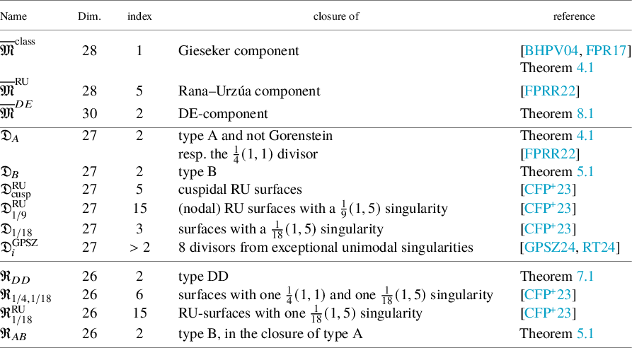

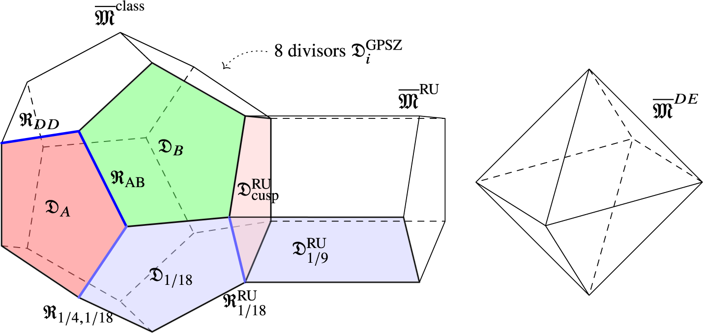

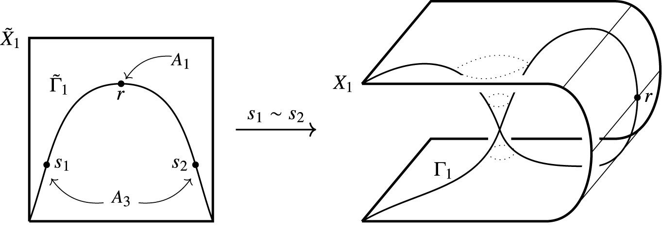


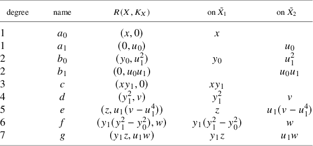

 Open access