Improvements for Twin Modeling

Since umx version 1.8.0, a dedicated summary method triggered by the user-facing umxSummary() function has been available. All SEM functions, including the twin analysis functions, now produce a publication-ready report if the model object is passed to umxSummary(). umxSummary() supports sorting parameters by type, reporting the fit indices, and provides interpretation guidelines for the fit indices’ values, and can output to LaTeX or html for pasting into a word processor. Another new reporting tool is umxSummarizeTwinData(), which produces publication-ready tables with means and group correlations (MZs, DZs, and so on) for each variable stratified by twin pair type (all male, all female, and discordant pairs).

Modeling capabilities have also improved. Core functions such as umxACE now support adding covariates (both ordinal and continuous), multigroup specifications, and standardized reporting across twin ACE model, common pathway twin-model (CP), and simplex models. Additional features include support for gene–environment interaction (umxGxE_biv()), discordant twin designs (umxDiscTwin()), and power analysis tools (umxPower(), power.ACE.test()).

Integration and Graphical Specification

Interoperability has improved, whereby umxRAM() now accepts lavaan syntax. This allows specifying a umxRAM model as a lavaan string. Alternatively, models can be exported as a lavaan string, thereby integrating umx into the space of lavaan users.

Ωnyx is a free graphical user interface (GUI) tool for specifying structural equation models (SEMs) by drawing path diagrams interactively (von Oertzen et al., Reference von Oertzen, Brandmaier and Tsang2015). In umx v4.5, the Ωnyx exported path syntax can be directly read by umxRAM() or umxTwinMaker(). For twin models, the umxTwinMaker() can be used to transform Ωnyx-specified paths into an biometrical genetic ACE ‘twin model’ specification, enabling a workflow from the graphical interface to advanced modeling of twin and family data.

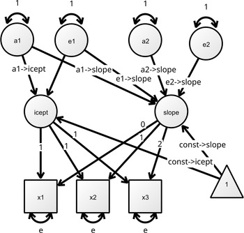
The listing below is the exported Ωnyx OpenMx path code from the diagram in Figure 1. The naming of the A, C, and E variances must follow the pattern (a1, a2, a3, etc.) so that umxTwinMaker() can appropriately set the MZ and DZ covariance paths and constraints to specify a version of the model adapted for twin data. Note: The data-related lines in the exported Ωnyx code (e.g., modelData <- read.table(…) and mxData(…)) must be commented out (or removed), because umxTwinMaker() automatically incorporates MZ and DZ data groups using the mzData and dzData arguments.

Figure 1. Ωnyx model diagram for a Cholesky AE specification. Notice the naming of the A and E variances should follow the pattern of a1, a2, a3, and so on, so that umxTwinMaker can set the remainder MZ/DZ paths and constraints for a twin model.

#

# This model specification was automatically generated by Onyx

#

# require(“OpenMx”);

# modelData <- read.table(DATAFILENAME, header = TRUE)

# manifests<-c(“x1”,“x2”,“x3”)

# latents<-c(“icept”,“slope”,“a1”,“e1”,

“a2”,“e2”)

# model <- mxModel(“umx2”,

# type=“RAM”,

# manifestVars = manifests,

# latentVars = latents,

lgc_paths <-c(

mxPath(from=“icept”,to=c(“x1”,“x2”,“x3”), free=c(FALSE,FALSE,FALSE), value=c(1.0,1.0,1.0), arrows=1,

label=c(“icept__x1”,

“icept__x2”,“icept__x3”)),

mxPath(from=“slope”,to=c(“x2”,“x3”), free=c(FALSE,FALSE), value=c(1.0,2.0), arrows=1, label=c(“slope__x2”,“slope__x3”)),

mxPath(from=“one”,to=c(“icept”,“slope”), free=c(TRUE,TRUE), value=c(1.0,1.0), arrows=1, label=c(“const__icept”,“const__slope”)),

mxPath(from=“a1”,to=c(“icept”,“slope”), free=c(TRUE,TRUE), value=c(1.0,1.0), arrows=1, label=c(“a1__icept”,“a1__slope”)),

mxPath(from=“e1”,to=c(“icept”,“slope”), free=c(FALSE,TRUE), value=c(1.0,1.0), arrows=1, label=c(“e1__icept”,“e1__slope”)),

mxPath(from=“a2”,to=c(“slope”), free=c(TRUE), value=c(1.0), arrows=1, label=c(“a2__slope”)),

mxPath(from=“e2”,to=c(“slope”), free=c(TRUE), value=c(1.0), arrows=1, label=c(“e2__slope”)),

mxPath(from=“x1”,to=c(“x1”), free=c(TRUE), value=c(1.0), arrows=2, label=c(“e”)),

mxPath(from=“x2”,to=c(“x2”), free=c(TRUE), value=c(1.0), arrows=2, label=c(“e”)),

mxPath(from=“x3”,to=c(“x3”), free=c(TRUE), value=c(1.0), arrows=2, label=c(“e”)),

mxPath(from=“a1”,to=c(“a1”), free=c(FALSE), value=c(1.0), arrows=2, label=c(“VAR_a1”)),

mxPath(from=“e1”,to=c(“e1”), free=c(FALSE), value=c(1.0), arrows=2, label=c(“VAR_e1”)),

mxPath(from=“a2”,to=c(“a2”), free=c(FALSE), value=c(1.0), arrows=2, label=c(“VAR_a2”)),

mxPath(from=“e2”,to=c(“e2”), free=c(FALSE), value=c(1.0), arrows=2, label=c(“VAR_e2”)),

mxPath(from=“one”,to=c(“x1”,“x2”,“x3”), free=F, value=0, arrows=1)#,

#mxData(modelData, type = “raw”)

);

lgc_model <- umxTwinMaker(

“lgc”,

paths = lgc_paths,

mzData = mzData,

dzData = dzData

)

The final OpenMx object lgc_model is a multiple groups model, with each submodel including the MZ and DZ specific data. This massively reduces scripting code for ACE models.

Joint Distribution Analyses: ICU Method

Censored data, where values fall below a limit of detection (LOD), are common in fields such as biomarker assays (bioassays), environmental monitoring, and other biological measurements. The Integrated Censored-Uncensored (ICU) method addresses this by treating below-threshold (censored) values as ordinal data and above-threshold values as continuous data, while assuming perfect correlation between the ordinal and continuous indicators within each individual. The expected covariance matrix is therefore singular. However, because any individual can only have one of the two scores (ordinal or continuous) this is readily handled using FIML estimation. The algorithm automatically trims the expected covariance matrix to contain only those rows and columns corresponding to the observed data vector. ICU modelling is a special case of censored data analysis for a pair of observed variables, where one variable is a binary with values falling below some threshold of detection, and a second observed variable receives entries for above-threshold values. If there is an entry in one of these pairs of columns, the corresponding column has an NA. In umx, ICU modeling is supported via xmu_make_bin_cont_pair_data(), which prepares paired ordinal-continuous data for SEM analyses of data from either twins or unrelated individuals splitting variables at a user-specified censoring point, e.g., a limit of detection

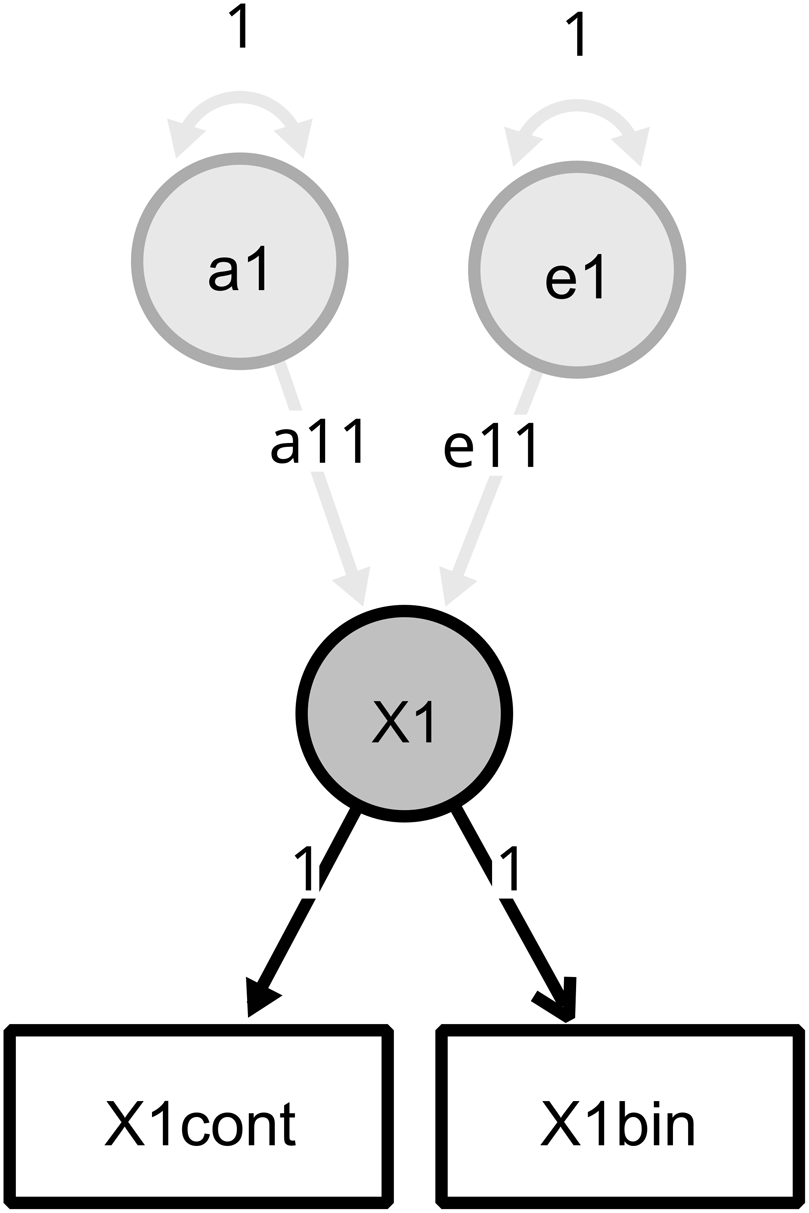
The example code below generates two new variables with the ‘bin’ and ‘cont’ suffixes (mpgbin, mpgcont): values below a chosen censoring point (0.001 in this example) are coded in mpgbin as an ordered factor level labeled <low> (creating a binary ordered variable that can take values <low> or <high>), with NA assigned for values above 0.001. Conversely, mpgcont receives NA for values below 0.001 and the actual mpg value for those above it. The matching diagram (RAM) specification for a twin example can be seen in Figure 2.

Figure 2. Ωnyx model diagram for a ICU specification. The X1 variable was split using xmu_make_bin_cont_pair() into X1cont and X1bin, the X1 latent variance now results from the joint-distribution analysis and is further split into A and E variances in a twin design.

df = xmu_make_bin_cont_pair_data

(uncensored_data,

vars = c(“X1”),

censp = 0.001, # the LOD

suffixes = c(“_T1”, “_T2”)) # if twin data

After preparing the paired binary and continuous data with xmu_make_bin_cont_pair_data(), in which the ‘censp’ argument splits variables at a user-specified value (without setting or fixing the model thresholds), the data are then incorporated into the model (e.g., via umxRAM() or a twin function). The threshold for each binary (censored) variable must be explicitly fixed with a user-specified value in the model’s threshold deviations matrix:

model$MZ$deviations_for_thresh$values[, c(“X1bin_T1”,“X1bin_T2”)]<- 0.001

model$MZ$deviations_for_thresh$free[, c(“X1bin_T1”,“X1bin_T2”)]<- FALSE

This approach reduces the need for data transformation, as it uses information available (threshold level) provided in the blood essay.

Covariate Placeholder for Definition Variables

Definition variables are additional variables that can be used directly in the specification of expected means or covariances. A common use case is ordinal data, where definition variables can be used to model the effects of covariates on outcomes of interest either at the latent trait level or directly on the item threshold(s). Both approaches are supported: regressing the latent mean shifts the underlying liability distribution, whereas regressing the thresholds adjusts boundaries conditional on the covariate (often expressed as threshold deviations). However, when using definition variables, rows with one or more missing definition variables are row-wise deleted. As it is well known in linear regression, row-wise deletion has adverse consequences for parameter estimates when data are either missing at random or not in the Little and Rubin (Reference Little and Rubin2014) sense. This problem is exacerbated in the case of data collected from pairs of relatives; for example, one twin has complete data on the dependent variables and definition variables, but the cotwin is missing the definition variable (even if phenotype data are available for that cotwin). The missing data on their cotwin’s definition variable forces the exclusion of the entire pair’s data from the analysis. This is undesirable for two reasons. First, there is waste of the data on the first relative. Second, including all valid data may help to correct estimates for volunteer bias (Neale & Eaves, Reference Neale and Eaves1993).

The function xmu_update_covar() prevents unnecessary row deletions in twin data by inserting a placeholder value into a twin’s covariate column only when that twin is missing the covariate (NA) but their cotwin has a nonmissing value for it. The placeholder chosen is the numeric value 99999, which will be automatically interpreted by the optimizer as an outlier and not affect the row’s likelihood calculation. In the event of a coding error (as might occur when processing such data manually), such as using 99999 for the covariate value when there are observed dependent variables for the cotwin, extreme parameter estimates and model-fitting issues are likely to be found, flagging the error to the user.

data(docData)

df = docData

# Add some missing data

df$varA1_T1[1:5] <- NA

df <- xmu_update_covar(df, covar = “varA1”, pheno = “varB1”)

head(df)

> zygosity varA1_T1 varA2_T1 varA3_T1 varB1_T1 varB2_T1 varB3_T1

> 1 MZMM 99999 0.409 -0.449 NA 2.580 1.467

> 2 MZMM 99999 -0.765 -1.583 NA -0.361 0.087

> 3 MZMM 99999 0.024 1.368 NA -0.859 -0.967

> 4 MZMM 99999 1.048 1.069 NA -0.433 0.307

> 5 MZMM 99999 1.393 2.719 NA 0.683 0.715

> 6 MZMM -0.672 0.918 1.467 -1.388 -0.555 0.494

Residualizing Covariates in Long and Wide Data: umx_residualize

umx_residualize() provides a concise, reliable way to residualize one or more dependent variables (DVs) on covariates, returning the original data frame with those variables replaced by their residuals. It supports (1) a familiar rbase formula interface and (2) fully supporting residualisation on wide-format twin data via suffixes automatically applying the same residualization to _T1, _T2, etc. columns. Internally, it wraps lm(…, na.action = na.exclude) and writes residuals back ‘in place’, saving boilerplate model setup and assignment code.

Residualization is appropriate for continuous outcomes when you want to partial out exogenous covariates before SEM/twin modeling (e.g., age, sex, scanner). For ordinal outcomes, definition variables are to be preferred, as residualization is not defined on the latent liability scale used by threshold models. OpenMx handles ordinals via thresholds and modeling the effect of definition variables on the latent trait, rather than regressing them out prior to analysis. Notice, however, that pre-residualizing covariates or using definition variables comes with the assumption that those covariates are exogenous and measured without error; if that assumption fails, bias will propagate to downstream parameters.

The interface to umx_residualize() is designed to be consistent with the formulae used in lm() and other R packages. The primary operators are ∼ for regressed on, + for main effects, and * for interactions; for example, y ∼ age * sex.

# (1) Residualize a single DV (mtcars example)

res1 <- umx_residualize(“mpg”, covs = c(“cyl”, “disp”), data = mtcars)

# (2) Formula interface, including non-linear terms and interactions

res2 <- umx_residualize(mpg ∼ cyl + I(cyl^2) + disp, data = mtcars)

# (3) Residualize multiple DVs at once

res3 <- umx_residualize(var = c(“mpg”, “hp”), covs = c(“cyl”, “disp”), data = mtcars)

# (4) Residualize *wide* twin data by suffixes

tmp <- mtcars

tmp$mpg_T1 <- tmp$mpg_T2 <- tmp$mpg

tmp$cyl_T1 <- tmp$cyl_T2 <- tmp$cyl

tmp$disp_T1 <- tmp$disp_T2 <- tmp$disp

tmp <- umx_residualize(var = “mpg”, covs = c(“cyl”, “disp”),

suffixes = c(“_T1”,“_T2”), data = tmp)

This example uses the common “mtcars” dataset for accessibility to the widest set of users, but twin modelers should see that the same flexibility applies to wide twin data by simply setting the twin suffix parameter.

Random Intercept Cross-Lagged Panel Model (RI-CLPM)

The RI-CLPM, introduced by Hamaker et al. (Reference Hamaker, Kuiper and Grasman2015), addresses a limitation of traditional CLPMs: the conflation of within-person dynamics with stable between-person differences. Standard CLPM (Castro-de-Araujo et al., Reference Castro-de-Araujo, de Araujo, Morais Xavier and Kanaan2023; Heise, Reference Heise1970) assumes that cross-lagged effects reflect causal processes, but these estimates are biased if individuals differ in trait-like levels of the variables. RI-CLPM introduces random intercepts for each variable, capturing stable between-person variance. This isolates within-person fluctuations across time, so cross-lagged paths estimate dynamic processes rather than trait-like (between-person) confounds.

There are only a few causal inferential models available. Among these, the CLPM family of models is distinctive in that it includes temporality. Auto-regressive paths adjust the state of a variable in a previous moment in time, and any remaining variance is either measurement error, innovation, or a causal effect in the subsequent occasion (the cross-lagged path).

umx() provides a high-level function that simplifies CLPM specifications with and without RI. It also provides options to incorporate elements from instrumental variable (IV) methodology into the CLPM. Singh et al. (Reference Singh, Verhulst, Vinh, Zhou, Castro-de-Araujo, Hottenga, Pool, de Geus, Vink, Boomsma, Maes, Dolan and Neale2024) reported that the inclusion of instrumental variables in the context of CLPM provides extra degrees of freedom for within-wave causal inference, along with the cross-lagged paths. More recently, the Hamaker et al. (Reference Hamaker, Kuiper and Grasman2015) model was extended with instrumental variables (IV-RI-CLPM; Castro-de-Araujo, Singh, Zhou, Vinh, Kramer et al., Reference Castro-de-Araujo, Singh, Zhou, Vinh, Maes, Verhulst, Dolan and Neale2025), allowing within-wave causal investigation in the multi-level context, that is, separating trait-like and state-like variation. The IV-RI-CLPM model (Castro-de-Araujo et al., Reference Castro-de-Araujo, Singh, Zhou, Vinh, Maes, Verhulst, Dolan and Neale2025), as well as standard CLPM (Castro-de-Araujo et al., Reference Castro-de-Araujo, de Araujo, Morais Xavier and Kanaan2023; Heise, Reference Heise1970), and RI-CLPM (Hamaker et al., Reference Hamaker, Kuiper and Grasman2015) specifications are available in umx v4.5.

data(docData) # example panel data

dt <- docData[2:9] # select 4 waves for X and Y

m_clpm <- umxCLPM(

waves= 4,

name = “Hamaker2015”,

model = “Hamaker2015”,

data = dt,

autoRun = TRUE

)

umxSummary(m_clpm)

Mendelian Randomization and MR-DoC

Mendelian Randomization (MR) uses genetic variants as instrumental variables to estimate causal effects between phenotypes in the presence of background confounding. umx not only includes a basic MR function umxMR, but also more sophisticated models capable of incorporating measured genetic data in twin designs. MR-DoC extends MR by combining instrumental variables and the direction-of-causation (DoC) model (Castro-de-Araujo, Singh, Zhou, Vinh, Maes et al., Reference Castro-de-Araujo, Singh, Zhou, Vinh, Maes, Verhulst, Dolan and Neale2025; Minică et al., Reference Minică, Dolan, Boomsma, de Geus and Neale2018). Because the cross-twin cross-trait correlations provide extra degrees of freedom, MR-DoC allows the estimation of direct pleiotropic paths or full background confounding. Umx provides two versions: MR-DoC (Minică et al., Reference Minică, Dolan, Boomsma, de Geus and Neale2018) estimates a direct pleiotropic path from the instrument to the outcome, but requires fixing unique environmental variance correlations between exposure and outcome for identification; and MR-DoC2 (Castro-de-Araujo et al., Reference Castro-de-Araujo, de Araujo, Morais Xavier and Kanaan2023), which can estimate causal paths in both directions (between exposure and outcome) while adjusting for all noncausal background confounding. MR-DoC2 does not permit direct pleiotropic path estimation. However, this exclusion restriction, whereby PRSs act solely through their intended phenotypes can be relaxed by imposing additional constraints. One approach is to fix the unique environmental correlation (re) to zero and set the unique environmental variances to 1. Alternatively, certain variance components can be fixed to zero, or other correlations depending on data structure. These constraints will allow the estimation of horizontal pleiotropy but at the cost of assuming no confounding from the fixed components. MR-DoC2 is also identified with non-twin siblings, with the necessary constraint of coalescing additive genetic (A) and shared environmental (C) variances into a single familial resemblance (F) component.

The package now provides variance components specifications of a simple DoC model, as well as the MR-DoC and MR-DoC2 extensions. The implementation permits easy model parsimony tests, and supports ordinal variables via a latent threshold liability scale.

# mzData/dzData should contain twin pairs + phenotypes & PRS columns

m_mrdoc <- umxMRDoC(

pheno = c(“BMI”, “SBP”), # exposure, outcome

prss = c(“PRS_BMI”), # single instrument, mrdoc

mzData = mz_df,

dzData = dz_df

)

umxSummary(m_mrdoc)

Definition Variables

A definition variable in OpenMx is a row-specific value that modifies the model for that observation. Unlike fixed parameters, definition variables allow per-subject moderation of means, variances, or paths. In umx v4.5, definition variables can be specified directly in umxRAM() using umxPath(defn = “defvar”). This avoids manual algebra specification and supports continuous moderators without grouping. All subsequent references to the definition variable should include the def_ prefix, as in umxPath(from=”def_defvar”, to = “X1”). This syntax corresponds to a specification where the definition variable affects the means of X1.

Definition variables are the only appropriate option when working with ordinal variables, since ordinal variables should not be residualized. In psychology and psychiatry research, ordinal variables often comprise the majority of available data. Therefore, the availability of this feature in the engine, OpenMx, is fundamental for research in these fields.

Currently, only OpenMx and MPLUS (Muthén & Muthén, Reference Muthén and Muthén2011) offer definition variables in SEM. Its use has been fundamental in gene-by-environment moderation, where the most used method leverages a definition variable to estimate the moderating effect (Purcell, Reference Purcell2002). Umx has provided tools for that specification since inception and includes plotting facilities (Bates et al., Reference Bates, Maes and Neale2019). With the defn syntax, such moderations can be concisely included in any RAM/path specification. For the twin models, umx v4.5 provides a utility for placeholder inclusion (discussed earlier) to avoid deleting rows for which only one of the twins has data in the definition variable cell.

Multigroup Sex-Limitation Twin Models: umxSexLim

umxSexLim() also implements multivariate sex-limitation twin models in a correlated-factors framework across five groups (MZ male, DZ male, MZ female, DZ female, DZ opposite-sex). This function enables the testing of (a) quantitative differences (sex-specific magnitudes of A, C, E) and (b) qualitative differences (distinct factors operating in one sex but not the other) while preserving identification for the DZ opposite-sex group via cross-sex correlations.

umxSexLim offers three nested specifications: nonscalar sex limitation, scalar sex limitation, and homogeneity. Nonscalar sex limitation allows for quantitative and qualitative sex differences on either A or C variances, with sex-specific intertrait correlations Ra, Rc, Re, and free male–female correlations in the DZ opposite-sex (DZOS) group. Scalar Sex Limitation allows only quantitative differences (distinct male/female paths), but a single set of Ra, Rc, and Re shared across sexes. Homogeneity corresponds to the baseline ACE assumption (equal A, C, E structures across sexes; means are free to differ).

Due to limits in degrees of freedom in the classical twin study, qualitative differences can be modeled for only one of A or C (A_or_C = “A” or “C”). The function defaults to A (dzAr) and C (dzCr) variance correlations of .5 and 1, respectively, which can be changed to test alternative models (e.g., dzCr = .25 for ADE). Assumptions typically include equating means/variances across birth order within zygosity groups. Finally, the umxSexLim() accepts ordinal phenotypes and configures the model object automatically. Local identification of models generated by the high-level functions can be assessed using the recent OpenMx function mxCheckIdentification() (Hunter et al., Reference Hunter, Kirkpatrick and Neale2025).

library(umx)

# Example data: anthropometry (included with umx)

data(“us_skinfold_data”)

# Base names of traits (suffixes define twins, e.g., _T1/_T2)

selDVs <- c(“tri”, “bic”, “caf”)

# Split data by zygosity/sex (columns already wide with _T1/_T2)

mzm <- subset(us_skinfold_data, zygosity == “MZMM”)

dzm <- subset(us_skinfold_data, zygosity == “DZMM”)

mzf <- subset(us_skinfold_data, zygosity == “MZFF”)

dzf <- subset(us_skinfold_data, zygosity == “DZFF”)

dzo <- subset(us_skinfold_data, zygosity == “DZOS”)

# Fit a Nonscalar model with qualitative differences on A

m_nsA <- umxSexLim(

name = “Skinfold_Nonscalar_A”,

selDVs = selDVs,

sep = “_T”, # base names + suffixes (_T1/_T2)

mzmData = mzm, dzmData = dzm, mzfData = mzf, dzfData = dzf, dzoData = dzo,

A_or_C = “A”, # qualitative differences modeled on A

sexlim = “Nonscalar”,

autoRun = TRUE

)

# Journal-ready summary (CIs, optional genetic/environmental correlations)

umxSummarySexLim(m_nsA, showRg = TRUE, report = “html”)