

1. INTRODUCTION
Jakobshavn Isbræ, Greenland's largest marine-terminating glacier, has doubled in speed as its ice front has retreated tens of km in the last several decades (Joughin and others, Reference Joughin, Abdalati and Fahnestock2004, Reference Joughin2008; Rignot and Kanagaratnam, Reference Rignot and Kanagaratnam2006; Howat and others, Reference Howat2011). Increases in subsurface melting and calving triggered by warmer ocean water are believed to be important contributors to this process (Holland and others, Reference Holland, Thomas, De Young, Ribergaard and Lyberth2008; Motyka and others, Reference Motyka2011; Enderlin and Howat, Reference Enderlin and Howat2013; Myers and Ribergaard, Reference Myers and Ribergaard2013; Truffer and Motyka, Reference Truffer and Motyka2016).
Modeling the calving process is challenging, and has produced conflicting results. A finite-element model of stress evolution near the front of marine-terminating glaciers suggests that undercutting of the ice front due to frontal melting near the base is a strong driver of calving (O'Leary and Christoffersen, Reference O'Leary and Christoffersen2013). However, a vertical 2-D ice flow model found that crevasse water depth and basal water pressure could have significant effects, while submarine melt undercutting and backstress from ice mélange are less important (Cook and others, Reference Cook2014). The models of Cook and others (Reference Cook2014) and many others (e.g., Nick and others (model CDw), Reference Nick, Van der Veen, Vieli and Benn2010; Otero and others, Reference Otero, Navarro, Martin, Cuadrado and Corcuera2010), use the calving criterion of Benn and others (Reference Benn, Hulton and Mottram2007), which assumes that calving happens when the depth of surface crevasses reaches the waterline, and does not require a basal crevassing condition. Recent work by Murray and others (Reference Murray2015a, Reference Murrayb) cast doubt on this calving criterion. Their data show that the front of Helheim Glacier tipped backwards during a major calving event, which implies that basal crevassing must be considered in calving criteria at least under certain conditions. Detailed observations of ice geometry and kinematics near the calving front can provide constraints on calving models. Amundson and others (Reference Amundson2010) used time-lapse imagery, GPS, ocean pressure and seismic observations at Jakobshavn Isbræ to demonstrate that sea ice coverage and the strength of mélange affect the seasonal variations in calving rate and terminus stability: the glacier terminus advances in winter when the dense and strong ice mélange prevents calving, and retreats in summer when the ice mélange becomes weak. A simple force-balance analysis suggested that when there is a resistive ice mélange, bottom-out rotation of the calving block is strongly preferred over top-out rotation. By using photogrammetric time-lapse imagery, Rosenau and others (Reference Rosenau, Schwalbe, Maas, Baessler and Dietrich2013) documented a major calving event at Jakobshavn Isbræ, finding large vertical displacements of the glacier front of order 15 m and lowering of order 8 m at a position 500 m from the calving front 2 d before the calving event, similar to the observations at Helheim Glacier by Murray and others (Reference Murray2015a, Reference Murrayb).
Terrestrial radar interferometry (TRI) allows detailed observations of the calving front, generating high-resolution elevation and velocity data with short (several minutes or less) repeat intervals (Dixon and others, Reference Dixon2012; Peters and others, Reference Peters2015; Voytenko and others, Reference Voytenko2015a, Reference Voytenkob, Reference Voytenkoc). With this instrument, we can measure glacier motion and map ice velocity and elevation over a wide area, overcoming the limitations of GPS (low spatial resolution, difficult to deploy near the calving front), photogrammetry (low reliability in bad weather and at night), and satellite observations (low temporal resolution). Using continuous TRI observations near the terminus of Jakobshavn Isbræ acquired for 4 d in June 2015, we discuss the possible role of crevasses and basal melting before and during a calving event.
2. DATA ACQUISITION
We observed the terminus of Jakobshavn Isbræ with a TRI from June 6–10 2015. The instrument is a real-aperture radar operating at Ku-band (1.74 cm wavelength) and is sensitive to line-of-sight (LOS) displacements of ~1 mm (Werner and others, Reference Werner, Strozzi, Wiesmann and Wegmüller2008). The instrument was mounted on a metal pedestal on solid rock ~3 km away from the calving front, and protected by a radome to eliminate disturbance from wind and rain (Fig. 1). Figure 2 shows the area measured during 4 d of continuous observation. The TRI scanned a 150° arc at a sampling rate of 90 s, generating images with both phase and intensity information. The resolution of the range measurements is ~1 m. The azimuth resolution varies linearly with distance: for example, 7 m at 2 km distance, 14 m at 4 km.
TRI set-up at Jakobshavn Isbræ, Greenland. The instrument is inside the radome, the height of the radome is ~3 m. The calving front is ~3 km away.

TRI intensity image of the study area overlain on a Landsat-8 image (4 June 2015). The radar scanned a 150° arc. Blue line indicates the ice cliff, green triangle shows the location of the radar, dashed red rectangle outlines the area shown in Figures 3, 4a, 5a. The coordinates are in UTM zone 22 N.

TRI images before (a) and after (b) calving on 10 June 2015, for the area outlined by a red box in Figure 2. Green line indicates the ice cliff before calving, red line after calving. Image b was obtained 26 min after image a. Black areas are in radar shadow.

Daily ice velocity estimated by tracking motion of distinct features. Blue boxes in (a) outline areas shown in more detail in (b), (c). Length of arrows is on the same scale as the background TRI intensity images (they are in the same reference coordinate system, 1 pixel length = 10 m). Black areas are in radar shadow.

(a), Averaged elevation map overlain on a Landsat-8 image, red rectangles indicate areas with more detailed elevation data (b = mélange in (b); c = ice front in (c)). (b) Stacked elevation time series for mélange, grey dots represent elevation values for all pixels (10 m × 10 m size) within box b; red line shows mean elevation. Note that the mean is close to zero; RMS variation represents combined effects of tides, atmosphere delay and phase unwrapping errors. (c) Time-varying elevation for different points along a flow line in box c, arranged in order of increasing distance from front. Black arrow indicates time of large calving event on 10 June 2015.

The TRI has one transmitting antenna and two receiving antennas, which allow for repeat topographic mapping of fast moving glaciers (Strozzi and others, Reference Strozzi, Werner, Wiesmann and Wegmüller2012; Voytenko and others, Reference Voytenko2015a). The baseline length (vertical offset between the two receiving antennas) in this campaign was 60 cm.
3. DATA ANALYSIS AND RESULTS
We first converted unwrapped phases into elevation maps using a geodetic reference height on the stationary rock, then adjusted the elevation into a local height coordinate system relative to the mean water level in the fjord. The results were resampled into 10 m pixel spacing maps and georeferenced into UTM coordinates for further analysis.
The TRI captured several small calving events during its 4-d observation period, and one large calving event near the end. Here we focus on the large calving event. Figure 3 shows the intensity images before (a) and after (b) this event. Surface dimensions of the calved block are ~1370 m × 290 m.
For fast moving glaciers like Jakobshavn Isbræ, ice near the terminus can move over 30 m d−1, so the location of the calving front can change more than 120 m during 4 d of observation. This motion must be considered when analyzing elevation variations of the glacier front. Our radar data are acquired in a fixed Cartesian system, so a given ice particle at the surface of the glacier travels through this Cartesian coordinate system (Eulerian reference frame). For this study, it is also useful to consider a Lagrangian reference frame, where we track a given particle of ice through time. We converted our elevation time series, originally defined in an Eulerian frame, into a Lagrangian frame, as follows:
 $$H_{{\rm Lag}}(x_{{\rm Lag}},y_{{\rm Lag}})_{\rm t} = H_{{\rm Eul}}(x_0 + {\rm d}x,y_0 + {\rm d}y)_{\rm t}$$
where H Lag and H Eul are elevations in the Lagrangian and Eulerian frame, respectively; (x Lag, y Lag) are the coordinates in the Lagrangian system, set equal to the initial coordinates (x 0, y 0) at t 0 in the Eulerian frame; and dx and dy are the horizontal displacements (relative to t 0) of ice at time t in the Eulerian frame.
To obtain dx and dy in Eqn (1), we estimated ice motion by using the feature tracking method in OpenCV (http://opencv.org/). Figure 4 is an example of ice motion derived by tracking distinct features such as the edges of surface crevasses on TRI intensity images. The velocity of the ice mélange is quite variable since even small calving events can cause large mélange motion. The glacier motion is variable over hourly timescales, but is relatively consistent over longer (1 d) periods. The estimated speed near the calving front was ~34 m d−1 during our observations.
Topographic mapping with the TRI is based on the interferometric imaging geometries of the two receiving antennas and the various targets in the imaged swath (Strozzi and others, Reference Strozzi, Werner, Wiesmann and Wegmüller2012). Two steps are necessary to convert unwrapped phases into elevation maps. First, we need to estimate the ‘expected’ phase at the radar position based on the elevation difference between the instrument and the reference point. Second, an elevation map is derived from the phase difference between the ‘expected’ radar phase and the unwrapped phase map. Ideally, for the first step, if we choose a stationary point (e.g., rock) as the reference elevation point, the ‘expected’ phases of the radar at different times should be the same. In reality, however, the phase of the radar position estimated at different times can be slightly different because of measurement noise. Since we hope to exploit the time-varying DEM capability of our TRI instrument, we cannot rely on long time (hour-scale) averages of multiple DEMs to reduce random noise in the elevation estimates. This noise is mainly due to atmospheric propagation effects (especially from variable water vapour) and possible small variations in antenna orientation associated with the scanning motion of the radar (the radome eliminates antenna motion due to wind).
We corrected the elevation estimates in two stages. As described above, a first order correction is applied by subtracting the ‘expected’ phase differences from a stationary point on rock ~600 m away from the instrument. This corrects the majority of effects due to antenna wobble, but may not improve the elevation estimates in the areas of interest on the glacier, as these are farther from the radar, and the radar signal propagates through atmosphere that is spatially and temporally variable. In a second step, we use elevation estimates in the mélange immediately in front of the glacier (box b in Fig. 5a) to correct the DEM on the glacier near the calving front, since we expect noise sources in the two areas to be similar. Tidal signals in the mélange are of order 1 m in amplitude, below the noise level of the elevation estimates, and we assume that over the 4 d of observation, the mean elevation change in this area is close to zero (no large icebergs entered the area during this period until the studied calving event). The resulting RMS scatter in the mélange (box b) is 1.8 m (Fig. 5b), about the level expected given instrument noise, atmospheric effects and tides. The elevations on the nearby glacier change by amounts that are much larger, but have several ‘tears’ in the time series associated with phase breaks. The deviations from the mean height in the mélange are used to correct these phase breaks. The corrected elevations still exhibit changes across the glacier front that are up to an order of magnitude higher than the changes in mélange (Fig. 5c).
Figure 5a is an averaged elevation map overlain on a Landsat-8 image. Figure 5c shows the corrected elevation profiles of points separated by 10 m along an approximate flow line beginning near the cliff that calved during the main calving event. The black arrow indicates the time of calving on 10 June 2015. In the 4 d before the large calving event the elevation of the glacier front increased by up to 20 m, in a way that is consistent with a simple block rotation model, as described below. These results are similar to the findings of Murray and others (Reference Murray2015a) who studied Helheim Glacier with GPS and photogrammetry. They suggested that glaciers can calve by a process of buoyancy-induced crevassing, with ice down-glacier in zones of flexure rotating upward (bottom-out rotation) because of disequilibrium.
The pattern of elevation increases along a flow line close to the ice cliff can be explained as follows. Assuming block behaviour, as the frontal ice block begins to flex at the beginning of a calving event, elevations near the cliff initially increase and the basal crevasse evolves and widens. Once the ice block is significantly out of equilibrium, ice failure can happen rapidly. The ice flexure and crevasse growth are separate physical processes that can be mutually reinforcing. We simplified these processes with a model of a single rigid block undergoing rotation with no internal deformation. Figure 6 is a cartoon showing the process. The new TRI data allow us to describe the timing and geometry of this process in some detail.
Cartoon of simplified rigid block rotation model, showing how elevation temporarily increases at the glacier front and defining the three variables. (a) Initial state, showing block width W. Dashed line marks the breaking surface during calving. (b) Dashed red shape shows how the calving block rotates by angle θ. (c) Solid red shape shows that the calving block also slides downward by distance D, while rotating about a horizontal axis.

The surface width of the ice block, W, can be determined directly from the TRI intensity images before and after the calving event. On a cross section plane, for a point on the upper surface with initial distance of d 0 to the ice cliff, and initial elevation of h 0, the horizontal distance from this point to the cliff is:
 $$d = W - [(W - d_0)\cos \theta - (h_0 - H_0)\sin \theta ]$$
where H 0 is the initial height of the intersection axis (the top of the calving surface of Fig. 6a) and θ is the rotation angle. The expression for elevation is:
 $$h = (W - d_0)\sin \theta + (h_0 - H_0)\cos \theta + H_0 - D$$
where D is the downward motion of the ice block (Fig. 6). Equations (2) and (3) assume the ice block rotates about the intersection axis in a rigid way.
To test this model, we selected a profile along a line that is perpendicular to the calving surface (the angle between the profile and the flow line direction is ~ 33°), and estimated elevations along the profile at different times (Fig. 7). Our time-varying DEMs effectively represent 15 min time averages, and are generated as follows: For each time increment, we derive elevations from five scans on each side (total of ten scans, spanning 15 min) and take the median value. If there are no usable measurements within a given 15 min increment, then there are no elevation estimates for that time. For comparison, different colour-coded curves in Figure 7 show the best-fit estimates for a rigidly rotating ice block, allowing the block edge on the upstream side to shift downward on the new ice cliff as calving proceeds. Figure 8 plots the rotation angle as a function of time (Supplementary Fig. S1 plots the downward motion as a function of time). Note the sudden drop at ~28.5 h before the calving event, which coincides with the time that a small piece of ice on the edge of the calving block fell from the cliff (Fig. 9).
Elevation profiles on the calving ice block at different times (hours before the calving event). Profiles are taken along the cyan line on the inserted TRI image, which is perpendicular to the calving front (green line on the TRI image). Distance is from the point to the ice cliff before the calving event, vertical dashed grey line (right hand side) marks the distance of the cliff after the calving event (red line on the TRI images). Markers show observed elevations on different times. Red curve is the best fit of a logarithmic function to the elevation profile at −80 h. Other colour-coded curves are the best-fit profiles at different times obtained by rotating the red curve about the intersection point on the dashed grey line and shifting it up or down to fit the observed elevations. Up-glacier side was shadowed by the higher down-glacier side so it is not possible to measure the surface subsidence here with this LOS radar.

Ice block rotation angle versus time. Blue dots are rotation angle estimates; red dots are rotation angles corrected by adding a Heaviside (H) step function after an ice failure event ~28.5 h before the main calving event (equation, upper left). Green and black curves are the best fits to the rotation time series before and after correction, assuming simple parabolic behaviour. Supplementary Fig. S1 shows downward motion versus time.

A small piece of ice on the cliff fell down ~28.5 h before the major calving event. (a) and (b) are TRI intensity images before and after this minor event. Red arrows indicate the location of ice fall. Note new ice blocks in the mélange and new cliff. Cyan lines show the profile of the ice block analyzed in this study. Time is in UTC.

Rosenau and others (Reference Rosenau, Schwalbe, Maas, Baessler and Dietrich2013) used time-lapse photography to suggest that vertical displacements of the glacier front at Jakobshavn Isbræ began ~2 d before a calving event. From Figure 7 and 8, we conclude that the calving process for our studied event actually started at least 65 h prior to the visually observed calving event.
4. DISCUSSION
Our simple block rotation model describes glacier front motion several days prior to a major calving event. The model has just three parameters: block width (W), rotation angle (θ) and downward motion of the up-glacier edge of the block (D). W is determined directly from the intensity images, while θ and D are determined by fitting the elevation time series data with model predictions. Figures 7, 8 show that the ice block started rotating at least 65 h before the calving event, a clear strain precursor to subsequent ice failure. The cross-over points in Figure 7 define an approximate lower bound for the width of the future calved block. Figure 7 also suggests that the elevation of ice close to the rotation axis decreases during the later stages of the calving process. The TRI intensity images support this: the observable ice surface becomes narrower as the up-glacier ice subsides and is shadowed by the higher down-glacier ice (Supplementary Fig. S2).
4.1. The role of subsurface melting
By studying tidal responses with photogrammetric time-lapse images, Rosenau and others (Reference Rosenau, Schwalbe, Maas, Baessler and Dietrich2013) found a narrow floating zone near the frontal cliff of Jakobshavn Isbræ. Our TRI-derived ice velocity estimates and phase lags relative to ocean tides suggest a ~1 km wide floating zone near the terminus during the observation period (Supplementary Information). The studied calving event happened at the front of this zone. Ice in the floating zone experiences tidal flexing, which can initiate Mode 1 (opening) cracks. These can form as both surface and basal crevasses. While surface crevasses can grow rapidly during a summer, basal crevasses can probably grow more rapidly if warm water is circulating in the fjord, reflecting the higher heat capacity of water relative to air.
Luckman and others (Reference Luckman2015) suggest that glacier undercutting driven by warm ocean temperature is an important process that contributes to calving in marine-terminating glaciers. We hypothesize that at the floating zone, where subsurface melting is likely faster than surface melting, the ice block moves out of gravitational equilibrium, which flexes the ice in a narrow zone (within which the new calving front will eventually form). As ice in this narrow zone flexes and the block rotates, crevasses enlarge, deforming zones narrow and strain increases exponentially. Eventually a failure threshold is reached and the block collapses. Figure 10 sketches the process. This model also explains the step change in elevation and rotation angle ~28.5 h before the calving event (Fig. 8): the preliminary ice fall removed mass above the water line, allowing the block to temporarily rebound. Continued subsurface melting eventually allowed the process to continue.
Sequential sketches of the physical process for calving. (a) Ice near calving front is neutrally buoyant. (b) Submarine melting exceeds surface melting, hence the ice block is no longer gravitationally stable. (c) Ice block sinks and rotates, basal crevasse enlarges, and the block eventually calves.

We can test this hypothesis by considering the differential stress generated by plausible amounts of subsurface melting, and comparing with laboratory-measured strength of ice. This analysis (see Supplementary Information) suggests that losses of order 30% are required to generate buoyancy-related differential stresses sufficient to initiate failure. This seems high, although ice in the terminal zone may be significantly weaker than laboratory-derived values, depending on the depth of pre-event crevassing. Perhaps a combination of surface and basal crevassing is necessary.
4.2. Ice failure model
Voight (Reference Voight1988) described a method for predicting material failure in rocks, soil and other solids under stress:
 $$\dot \Omega ^{-\alpha} \ddot \Omega = A$$
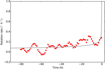
where A and α are empirical constants, Ω is an observable quantity related to deformation, and one and two dots refer to the first and second derivatives with respect to time. We suggest this model can also be applied to calving ice. We applied the model to the rotation of the ice block at Jakobshavn Isbræ, with Ω taken as the rotation angle θ, and the rotation rate $\dot \theta $
assumed to be infinite at the time of calving. By using a grid search approach, A and α were estimated to be 23.4 and 4.5. Following Voight (Reference Voight1988), the expression for rotation rate when α >1 is:
$\dot \theta $
assumed to be infinite at the time of calving. By using a grid search approach, A and α were estimated to be 23.4 and 4.5. Following Voight (Reference Voight1988), the expression for rotation rate when α >1 is:
 $$\dot \theta = [A(\alpha - 1)(t_{\rm f} - t) + \dot \theta _{\rm f}^{1 - \alpha} ]^{1/(1 - \alpha )}$$
where subscript f indicates the time of failure. Figure 11 shows the block rotation rate versus time. The weighted root mean square (WRMS, where weights of rates are based on misfits to the rotation model) of the residuals between observations and model predictions, is 0.07° h−1. With the estimates of A and α, the observed quantity (rotation angle or downward motion) can be expressed as (Voight, Reference Voight1988):
 $$\eqalign{\theta &= \displaystyle{1 \over {A(\alpha - 2)}} \Bigg\{[A(\alpha - 1)(t_{\rm f} - t_0) + \dot \theta _{\rm f}^{1 - \alpha} ]^{2 - \alpha /1 - \alpha} \cr & \quad \quad \quad \quad \quad \quad - {[A(\alpha - 1)(t_{\rm f} - t) + \dot \theta _{\rm f}^{1 - \alpha} ]}^{2 - \alpha /1 - \alpha}\Bigg\}}$$
We add a Heaviside step function to account for the small ice failure event ~28.5 h before the main calving event. For downward motion, the values of A and α are estimated to be 1.1 and 4.3. Based on these estimates and the model, we can derive the elevations of selected points at time t before the calving event. Figure 12 is a plot of TRI-derived elevations and predictions based on the ice failure and block rotation models. The rotation angles and downward motions are computed by Eqn (6), assuming t 0 = −80 h. The profile locations and elevations are computed from Eqns (2) and (3).
Ice block rotation rate (red dots) versus time. At time 0 the iceberg collapses and we assume the rotation rate is infinite. Grey curve is the best fit of ice failure model with A and α equal to 23.4 and 4.5, respectively. WRMS residual of model fit is 0.07° h−1; weights of rates are based on misfits of the rotation model shown in Figure 7. Rotation rate estimates are based on rotation angles shown in Figure 8, using a least-squares smoothing filter (Gorry, Reference Gorry1990), with smoothing window =5 and local polynomial approximation of order =2. Note that the model fits both the rotation rate data as well as the calving time data.
Elevations from model predictions and TRI observations at different times (hours before the calving event). Distance is from the point to the ice cliff before the calving event, vertical dashed grey line (right hand side) marks the distance to the new ice cliff. Red curve is the best fit of a logarithmic function to the elevation profile at −80 h; other curves are elevation estimates based on the model. Markers show observed elevations at different times. The rotation angles θ (in degrees) and downward displacements D (in meters) from the model at different times are shown on the lower right.

The ice failure model parameters are sensitive to observations immediately before the calving event. Due to limited data quality, the uncertainties of the model predictions are relatively high. Note that the model ignores tidal forcing and assumes no internal deformation in the calving block. Analysis of tidal variations in the fjord shows no evidence that block rotation or ice failure are sensitive to tide or tide rate, but tidal flexing of the ice in the floating zone could extend the depth of crevasses and fracture and weaken the ice (see Supplementary Information). Improved precision in the time-varying elevation estimates, better estimates of local tides, and detailed block shape variations should allow for a better understanding of ice flexure during calving.
5. CONCLUSIONS
We used TRI-derived digital elevation models to investigate the behaviour of the calving front at Jakobshavn Isbræ. Ice elevation near the cliff began to increase several days before a major calving event on 10 June 2015. A simple rigid block rotation model matches the elevation profiles and suggests that block capsizing started ~65 h prior to calving. Subsurface melting in excess of surface melting may over-weight the above-water mass of ice and enhance crevasses, leading to ice deformation, block rotation and eventual ice failure. A simple failure model fits the rotation data quite well.
SUPPLEMENTARY MATERIAL
The supplementary material for this article can be found at http://dx.doi.org/10.1017/jog.2016.104.
ACKNOWLEDGEMENTS
This research was partially supported by NASA grant NNX12AK29G to THD. DMH acknowledges support from NYU Abu Dhabi grant G1204 and NSF grant ARC-130413.7. We thank Martin Truffer and an anonymous reviewer for their valuable comments.


 Open access