


1. Introduction
Radio frequency interference (RFI) has become an increasingly severe challenge for radio astronomy, driven by the growing sensitivity of modern telescopes and the proliferation of human-made radio sources. Time-domain sciences like pulsar and fast radio burst (FRB) searches often rely on high time-resolution observations, which can be significantly impacted by both impulsive and persistent RFI. Moreover, identifying and masking RFI in such observations can demand substantial computational resources. Consequently, the development of effective and efficient RFI mitigation algorithms is crucial for maximizing the scientific outputs of astronomical data.
Over the years, numerous RFI mitigation strategies have been proposed, including frequency-domain approaches such as the use of notch filters, time-domain techniques such as data flagging, and telescope-level measures such as the establishment of radio-quiet zones (Fridman & Baan Reference Fridman and Baan2001; Briggs & Kocz Reference Briggs and Kocz2005; Gary, Liu, & Nita Reference Gary, Liu and Nita2010; Baan Reference Baan2019). Among these, threshold-based methods are the most widely adopted due to their simplicity and efficiency (e.g. Ransom, Eikenberry, & Middleditch Reference Ransom, Eikenberry and Middleditch2002; Offringa et al. Reference Offringa2010; Zeng et al. Reference Zeng2021). More advanced techniques, such as median filtering and SumThreshold algorithms, have also been developed to enhance RFI detection (Bhat et al. Reference Bhat, Cordes, Chatterjee and Lazio2005; Offringa et al. Reference Offringa2010; Zeng et al. Reference Zeng2021). However, these methods often struggle with weak and persistent RFI and are limited by fixed time-frequency resolution settings (Baan, Fridman, & Millenaar Reference Baan, Fridman and Millenaar2004).
Machine learning approaches represent a promising new direction in RFI mitigation. Techniques such as convolutional neural networks (CNNs) and U-Net architectures have been employed to automatically learn and classify RFI features (Akeret et al. Reference Akeret, Chang, Lucchi and Refregier2017; Burd et al. Reference Burd2018; Kerrigan et al. Reference Kerrigan2019; Vafaei Sadr et al. Reference Vafaei Sadr, Bassett, Oozeer, Fantaye and Finlay2020; Dao et al. Reference Dao2024). While these methods show great potential, they require large, labelled datasets for training, making them time-consuming and challenging to implement for large-scale observatories.
Radio observations conducted with multi-beam receivers or phased array feeds (PAF) offer a significant advantage for mitigating RFI, as most RFI signals are typically detected by multiple beams or pixels. In high time-resolution observations using multi-beam systems, spatial filtering techniques were explored by Kocz et al. (Reference Kocz, Briggs and Reynolds2010) for the 13-beam receiver on Murriyang, the Parkes 64-m radio telescope. Similar approaches have since been implemented for the 19-beam receiver system on the Five-hundred-meter Aperture Spherical radio Telescope (FAST) (Wang et al. Reference Wang2022). While spatial filtering has proven to be effective (Kocz et al. Reference Kocz, Briggs and Reynolds2010), it relies on the covariance matrix of multi-beam voltage data, which is generally unavailable for large-scale pulsar and FRB surveys.Footnote a As an alternative, the cross-correlation matrix (CCM) of multi-beam power data can be utilised to identify and mitigate RFI. For instance, Kocz et al. (Reference Kocz, Bailes, Barnes, Burke-Spolaor and Levin2012) applied singular value decomposition (SVD) to the CCM of frequency-averaged (at zero dispersion measure) time series from Murriyang’s multi-beam pulsar surveys, significantly reducing the number of false candidates. More recently, Chen et al. (Reference Chen2023) developed an RFI mitigation pipeline for FAST’s 19-beam surveys, employing the SumThreshold algorithm on the CCM to effectively manage RFI.
In this study, we expand upon the method developed by Kocz et al. (Reference Kocz, Bailes, Barnes, Burke-Spolaor and Levin2012), extending it to both the time and frequency domains to enhance the efficiency of RFI identification for multi-beam receivers and future PAF systems. The CCM is computed for each frequency channel and a specified integration time, and eigenvalue decomposition is applied to identify RFI across different beams. Additionally, we incorporate the Asymmetric Reweighted Penalised Least Squares (ArPLS) algorithm (Baek et al. Reference Baek, Park, Ahn and Choo2015) to fit and normalise bandpass, improving sensitivity to weak RFI. A publicly available package, called mRAID (multi-beam RAdio frequency Interference Detector), is provided alongside this paper. Section 2 outlines the dataset used in this study. In Section 3, we describe the key stages of our RFI identification methods, including bandpass normalisation, the construction of the CCM, and the application of the eigenvalue decomposition method. Section 4 details the implementation of the proposed approach on FAST data and discusses the results. Section 5 gives some conclusions.
2. Experimental data
To demonstrate the performance of mRAID, we used one observation from the FASTFootnote
b
19-beam receiver in the pulsar search mode, where PSR J1832+0204_P was discovered in beam 11 (Han et al. Reference Han2025). The observation has a time resolution of 49.152 $\unicode{x03BC}$
s and a frequency resolution of 122.07 kHz, spanning the range of 1 000–1 500 MHz (Jiang et al. Reference Jiang2020). The total integration time is 412.00 s, and there are a total of 8 192 sub-integrations in the file. Each sub-integration consists of
$\unicode{x03BC}$
s and a frequency resolution of 122.07 kHz, spanning the range of 1 000–1 500 MHz (Jiang et al. Reference Jiang2020). The total integration time is 412.00 s, and there are a total of 8 192 sub-integrations in the file. Each sub-integration consists of $1\,024\times4\,096$
data points, where 1 024 represents the number of sampling points per sub-integration, and 4 096 corresponds to the number of frequency channels. The data were 8-bit sampled and two polarisations were recorded.
$1\,024\times4\,096$
data points, where 1 024 represents the number of sampling points per sub-integration, and 4 096 corresponds to the number of frequency channels. The data were 8-bit sampled and two polarisations were recorded.
For the FAST 19-beam receiver, satellite and aircraft signals are the two primary sources of RFI. Satellite RFI typically occupies multiple frequency bands, with each band often shared by several satellites. These interferences are broadband and persist throughout the observation. In contrast, aircraft RFI contaminates only a few pixels in the time–frequency plane and lasts for a few seconds. Besides these known RFI sources, the data often include other narrowband, continuous, or intermittent interference signals.
3. RFI identification strategy
Our RFI identification scheme is designed based on three key components: the bandpass normalisation, the construction of the CCM, and the identification of RFI using eigenvalue decomposition. We describe each of these components in the following sections.
3.1. Bandpass normalisation using ArPLS
The signal level can vary considerably across different beams and frequencies, which can affect the performance of CCM-based RFI identification. To improve the robustness of the method, especially for identifying low-level RFI, bandpass normalisation is therefore highly beneficial. The ArPLS algorithm is a robust method tailored for this purpose, offering significant advantages over traditional approaches such as polynomial fitting or Gaussian filtering. By iteratively minimising a regularised least-squares function, ArPLS balances the need for accurately fitting the underlying signal and suppressing noise or RFI contamination. As demonstrated by previous studies (e.g. Zeng et al. Reference Zeng2021; Wang et al. Reference Wang2022), ArPLS outperforms conventional methods in both speed and accuracy, making it an ideal choice for large-scale surveys that require efficient bandpass normalisation as part of the RFI mitigation process.
To perform bandpass normalisation, we first aggregate the time-domain samples within a given time interval (e.g. 1.00 s) for each frequency channel. The bandpass shape is then fit using the ArPLS method. During normalisation, the fitted bandpass is subtracted from the time-domain data for each frequency channel. The correction is applied uniformly across all time samples, ensuring that the bandpass variations are consistently removed without altering the original resolution of the data.
3.2. The construction of CCM
After bandpass normalisation, we calculate the CCM for a given frequency channel (j) and subinterval (k), which is defined as
 \begin{align}C_\textrm{j,k} =\begin{pmatrix}\langle B_{j,k,1} B_{j,k,1} \rangle & \quad \langle B_{j,k,1} B_{j,k,2} \rangle & \quad \cdots & \quad \langle B_{j,k,1} B_{j,k,i} \rangle \\ \langle B_{j,k,2} B_{j,k,1} \rangle & \quad \langle B_{j,k,2} B_{j,k,2} \rangle & \quad \cdots & \quad \langle B_{j,k,2} B_{j,k,i} \rangle \\ \vdots & \quad \vdots & \quad \ddots & \quad \vdots \\ \langle B_{j,k,i} B_{j,k,1} \rangle & \quad \langle B_{j,k,i} B_{j,k,2} \rangle & \quad \cdots & \quad \langle B_{j,k,i} B_{j,k,i} \rangle\end{pmatrix}\end{align}
Here, $B_{j,k,i}$
represents the total power recorded from the i-th beam in channel j and subinterval k, which is a function of time. The number of time sample in
$B_{j,k,i}$
represents the total power recorded from the i-th beam in channel j and subinterval k, which is a function of time. The number of time sample in $B_{j,k,i}$
is
$B_{j,k,i}$
is $N_{ s}=T_{k}/t_\textrm{s}$
, where
$N_{ s}=T_{k}/t_\textrm{s}$
, where $T_{k}$
is the length of subinterval and
$T_{k}$
is the length of subinterval and $t_{s}$
is the sampling time. Each element in the matrix, denoted as
$t_{s}$
is the sampling time. Each element in the matrix, denoted as $\langle \cdots \rangle$
, represents the cross-correlation between two beams for a given subinterval k and channel j. The correlation matrix
$\langle \cdots \rangle$
, represents the cross-correlation between two beams for a given subinterval k and channel j. The correlation matrix $C_{j,k}$
is a square
$C_{j,k}$
is a square $N_\textrm{beam} \times N_\textrm{beam}$
matrix.
$N_\textrm{beam} \times N_\textrm{beam}$
matrix.
In multi-beam receiver systems, significant RFI often creates strong correlations between signals from different beams. Calculating the CCM provides an efficient way for identifying RFI while also improving sensitivity to low-level interference compared to algorithms that analyse each beam independently. By performing eigenvalue decomposition on the cross-correlation matrix of the multi-beam data, we can isolate these common structures, which are likely dominated by RFI.
3.3. The identification of RFI using eigenvalue decomposition
Eigenvalue decomposition is a matrix factorisation technique that decomposes a square $n\times n$
matrix into:
$n\times n$
matrix into:
 \begin{equation} C = Q \unicode{x1D6EC} Q^{-1},\end{equation}
where Q is a square $n\times n$
matrix whose ith column is the eigenvector
$n\times n$
matrix whose ith column is the eigenvector $q_{i}$
of C, and
$q_{i}$
of C, and $\unicode{x1D6EC}$
is a diagonal matrix whose diagonal elements are the corresponding eigenvalues,
$\unicode{x1D6EC}$
is a diagonal matrix whose diagonal elements are the corresponding eigenvalues, $\unicode{x1D6EC}_{ i,i}=\lambda_{i}$
. These eigenvalues are normalised by squaring them and dividing by the sum of all squared eigenvalues, ensuring that the eigenvalues reflect the proportion of variance explained by each eigenvector. The eigenvalues in
$\unicode{x1D6EC}_{ i,i}=\lambda_{i}$
. These eigenvalues are normalised by squaring them and dividing by the sum of all squared eigenvalues, ensuring that the eigenvalues reflect the proportion of variance explained by each eigenvector. The eigenvalues in $\unicode{x1D6EC}$
are ordered by magnitude, from the largest to the smallest (
$\unicode{x1D6EC}$
are ordered by magnitude, from the largest to the smallest ( $\lambda _1 \gt \lambda _2 \gt \ldots \gt \lambda _i$
). Large eigenvalues correspond to the dominant features in the CCM, which are often attributed to RFI affecting multiple beams. The eigenvectors associated with these large eigenvalues allow us to identify beams most affected by these RFI.
$\lambda _1 \gt \lambda _2 \gt \ldots \gt \lambda _i$
). Large eigenvalues correspond to the dominant features in the CCM, which are often attributed to RFI affecting multiple beams. The eigenvectors associated with these large eigenvalues allow us to identify beams most affected by these RFI.
For a given subinterval and channel of an observation, mRAID calculates its CCM ( $C_{j,k}$
) and performs eigenvalue decomposition. The largest eigenvalue and its associated eigenvectors are stored in a HDF5Footnote
c
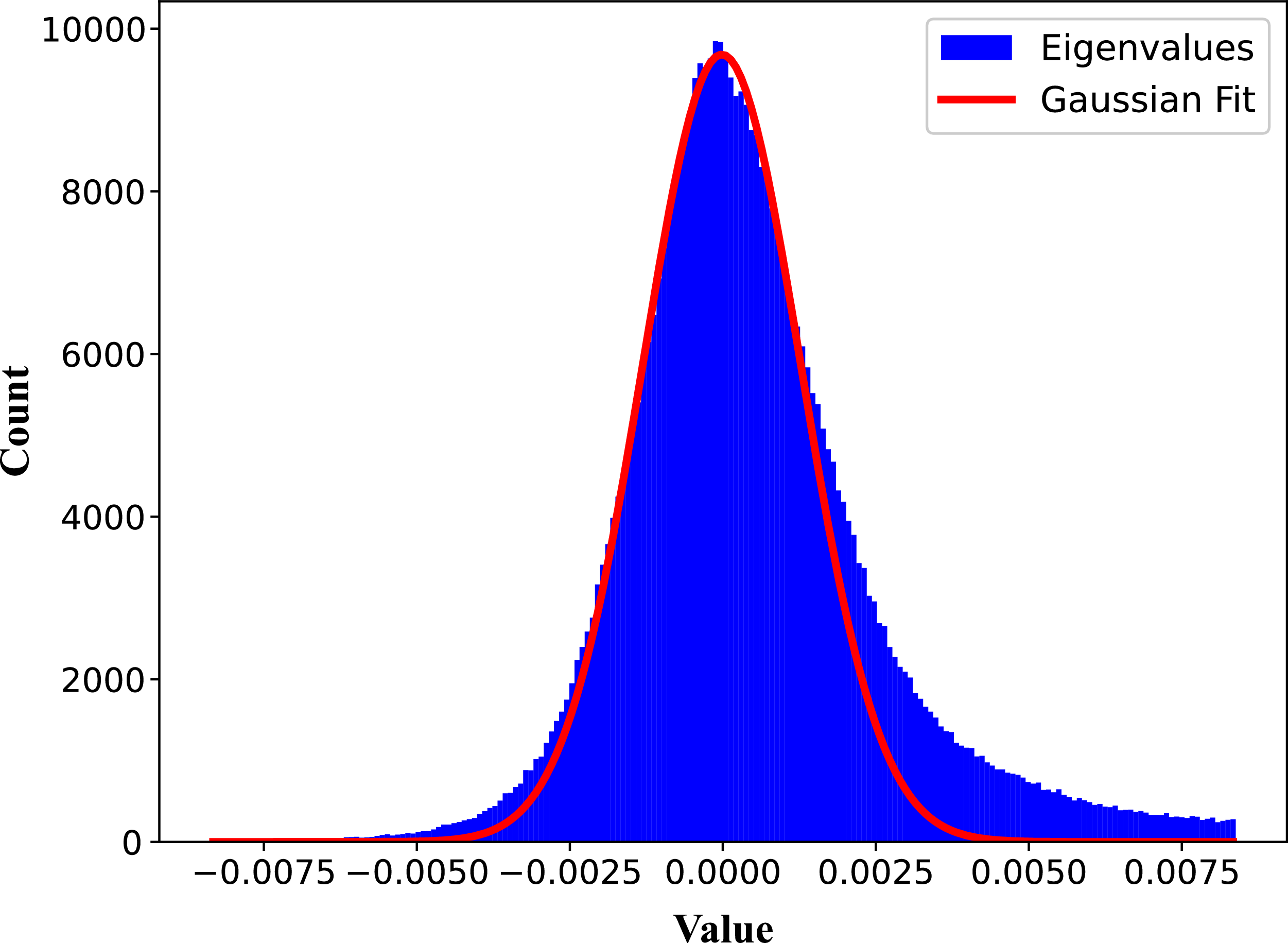
format file, to be further processed after the whole observation is completed. Such a process is completely independent for different subintervals and channels and can be carried out in parallel. Once the eigenvalue decomposition is finished for all subintervals, RFI-contaminated channels are identified through an iterative process that masks outliers in eigenvalues as a function of frequency and time (i.e. subinterval). The mean and standard deviation of eigenvalues are measured by performing a Gaussian fit to the distribution (see Figure 1), and iteratively masks channels with values exceeding a dynamic threshold. Once convergence is reached, a combined RFI mask is generated, capturing all identified RFI-contaminated channels and subintervals (see Figure 2).
$C_{j,k}$
) and performs eigenvalue decomposition. The largest eigenvalue and its associated eigenvectors are stored in a HDF5Footnote
c
format file, to be further processed after the whole observation is completed. Such a process is completely independent for different subintervals and channels and can be carried out in parallel. Once the eigenvalue decomposition is finished for all subintervals, RFI-contaminated channels are identified through an iterative process that masks outliers in eigenvalues as a function of frequency and time (i.e. subinterval). The mean and standard deviation of eigenvalues are measured by performing a Gaussian fit to the distribution (see Figure 1), and iteratively masks channels with values exceeding a dynamic threshold. Once convergence is reached, a combined RFI mask is generated, capturing all identified RFI-contaminated channels and subintervals (see Figure 2).
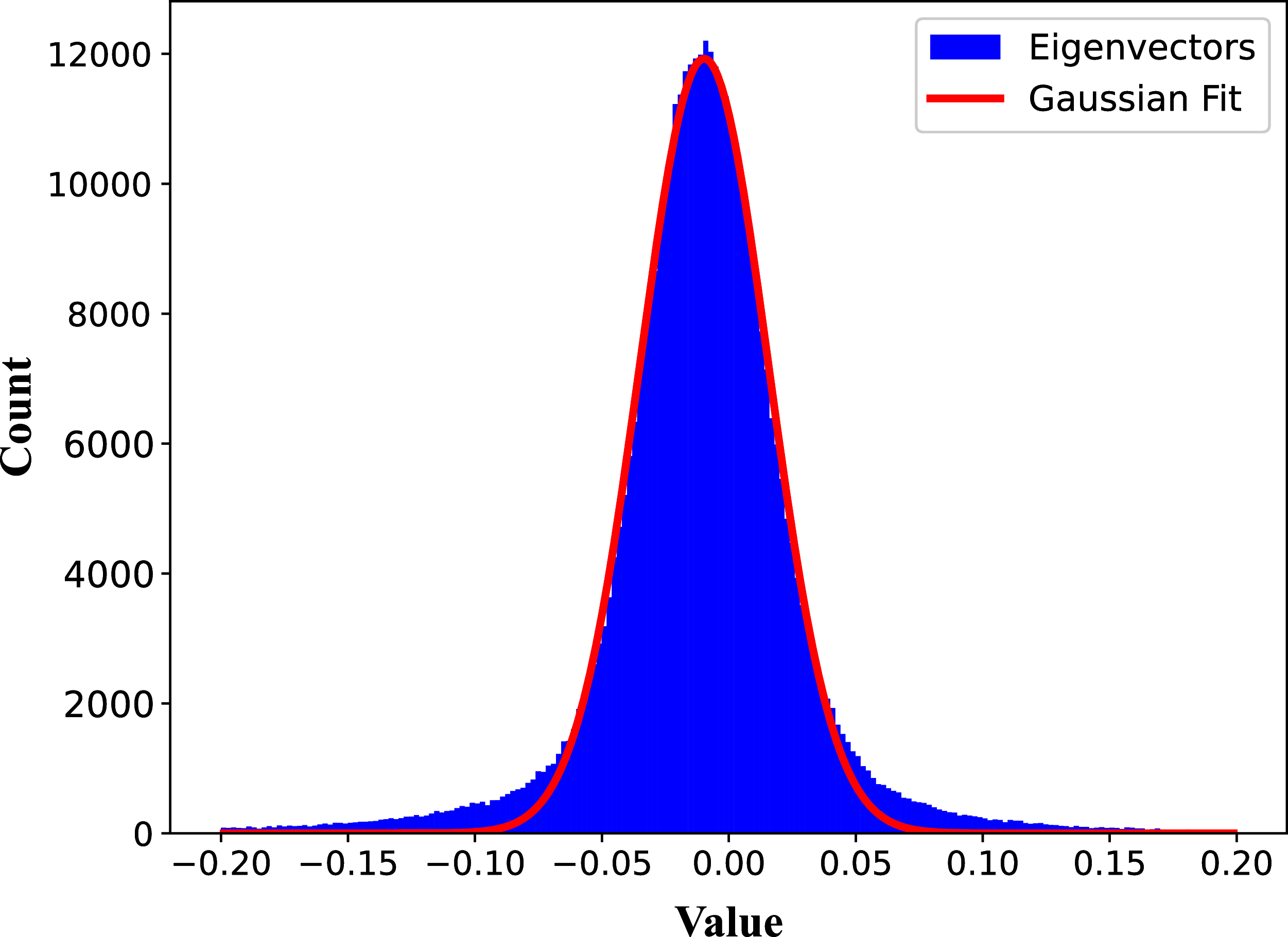
After masking eigenvalues, the next step involves using their associated eigenvectors to further confirm whether identified RFI channels are present across all beams. By applying a threshold to the elements of these vectors, the RFI detection process can be refined. If the magnitude of an element exceeds the threshold, the corresponding beam is considered to be strongly affected by RFI. Conversely, elements below the threshold indicate that the beams are unaffected and are classified as non-RFI channels. The threshold for the eigenvectors is determined individually for each beam by fitting a Gaussian distribution to the eigenvector elements of non-RFI channels specific to that beam as shown in Figure 3. This beam-specific approach ensures a more accurate classification of RFI channels tailored to the unique characteristics of each beam.
4. Experimental results and discussion
To evaluate the effectiveness of mRAID in identifying RFI, we performed a comparative analysis using observational data from the FAST 19-beam receiver. For comparison, we used rfifind, the RFI masking tool included in the widely used pulsar search software package PRESTO. Although several new tools have been developed specifically for FAST (e.g. Zeng et al. Reference Zeng2021; Wang et al. Reference Wang2022; Chen et al. Reference Chen2023), threshold-based methods, such as rfifind, remain the standard RFI mitigation tool for major FAST pulsar surveys (e.g. Li et al. Reference Li2018; Qian et al. Reference Qian2019; Han et al. Reference Han2021). As such, rfifind serves as an appropriate benchmark for assessing mRAID’s performance.
Histogram of dominant eigenvalues derived for all subintervals and channels of the FAST 19-beam test observation. A Gaussian fit to the distribution is shown as the red line.

4.1. Frequency domain RFI
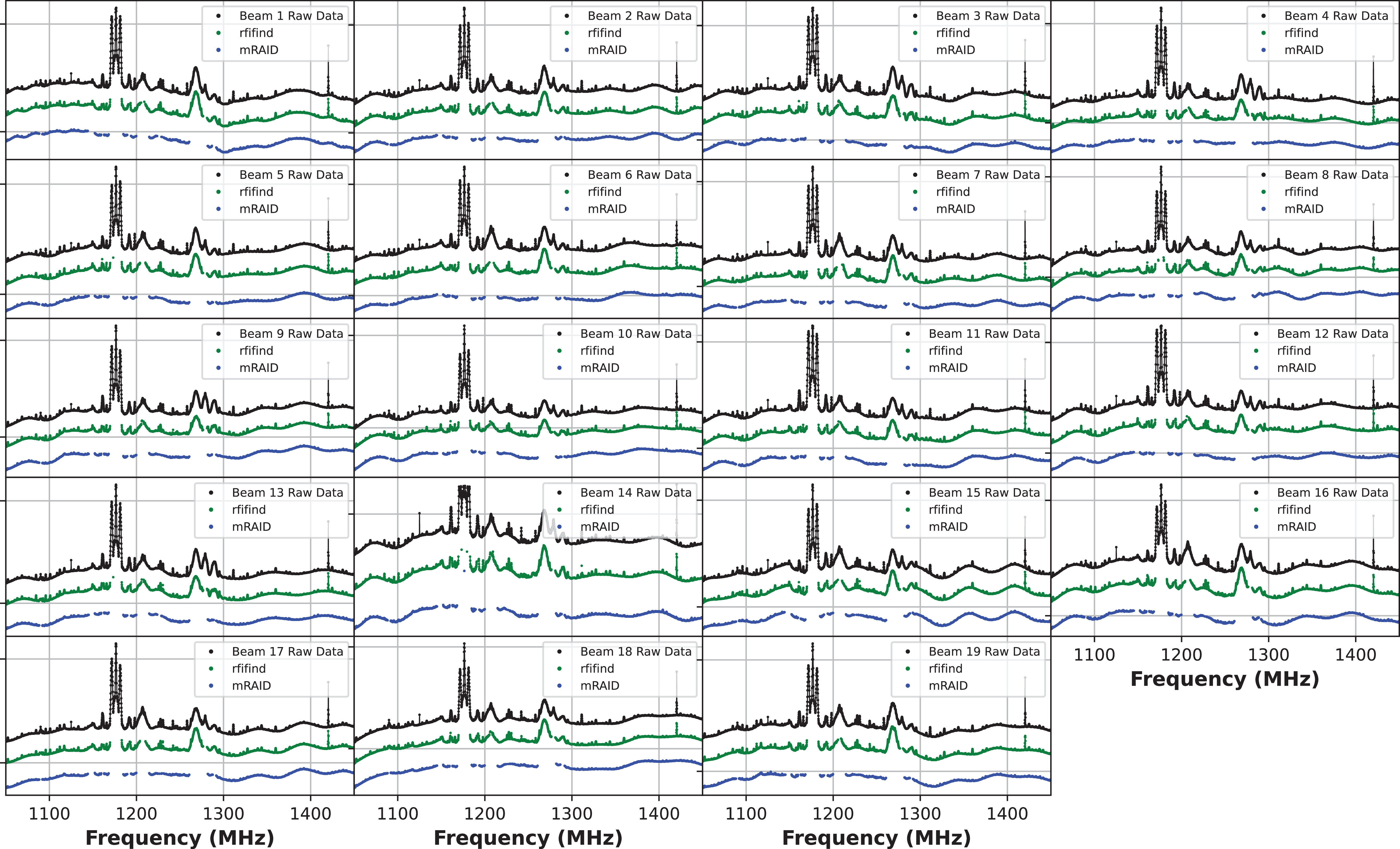
In Figure 4, we compare the bandpass of FAST observations before and after RFI masking. Each subplot corresponds to a single beam, displaying the time averaged bandpass of raw data (black points), RFI-masked data using rfifind (green points), and RFI-masked data using mRAID (blue points). The horizontal axis represents frequency channels, while the vertical axis indicates signal intensity on a log scale. Strong RFI contamination is evident in the raw data, characterised by sharp peaks at specific channels. For both rfifind and mRAID, the length of subintervals is 2.00 s. While rfifind identified strong RFI, residual contamination remains, particularly in highly affected regions. In contrast, mRAID achieved more effective RFI suppression, yielding cleaner bandpass.
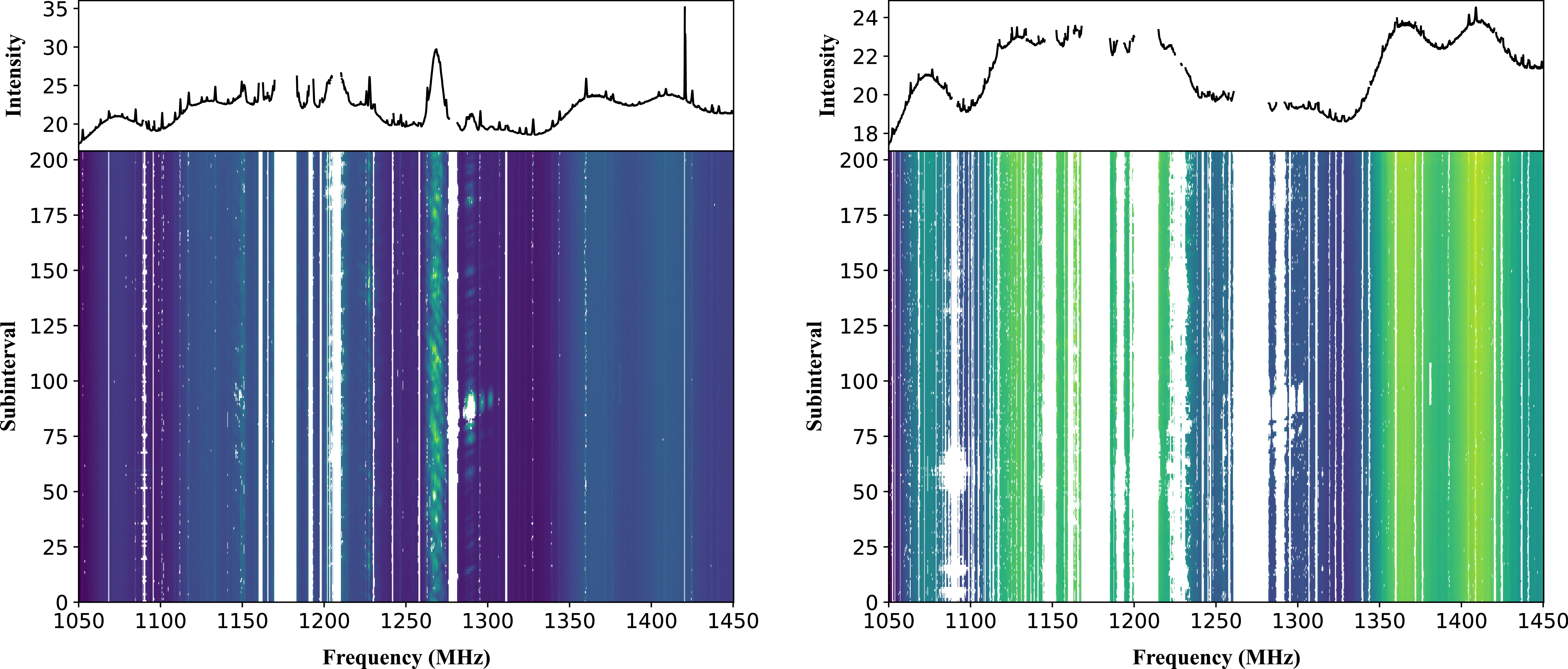
Figure 5 compares RFI masked data using rfifind (left panel) with that using mRAID (right panel) for beam 11, where PSR J1832+0204_P was discovered. The horizontal axis represents frequency channels, while the vertical axis denotes subinterval indices. Colour regions correspond to non-RFI data, whereas white regions indicate flagged RFI. The top panel in each subplot shows the average spectrum of the masked data. rfifind generated a less effective RFI mask, leaving some contaminated regions insufficiently flagged, for both narrowband (for example at $\sim1\,360$
MHz) and broadband (at
$\sim1\,360$
MHz) and broadband (at $\sim1\,270$
MHz) RFI. In contrast, mRAID exhibited a more effective RFI suppression in both narrowband and broadband cases, identifying and excising most interference.
$\sim1\,270$
MHz) RFI. In contrast, mRAID exhibited a more effective RFI suppression in both narrowband and broadband cases, identifying and excising most interference.
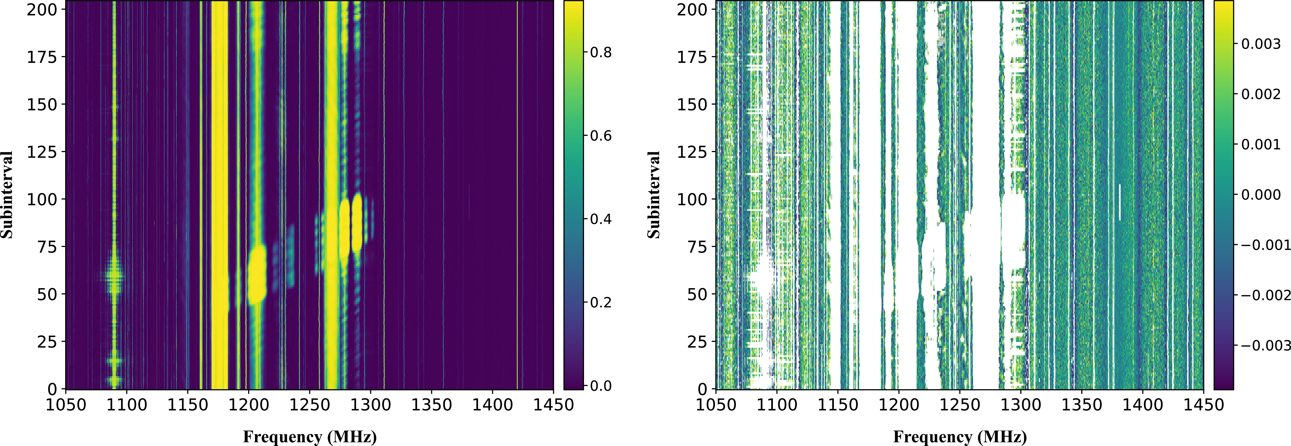
The left panel shows dominant eigenvalues derived for the FAST 19-beam test observation. The right panel shows the result after masking out RFI affected subintervals and channels, where the eigenvalue distribution becomes noise-like, indicating the effectiveness of the iterative RFI identification process.

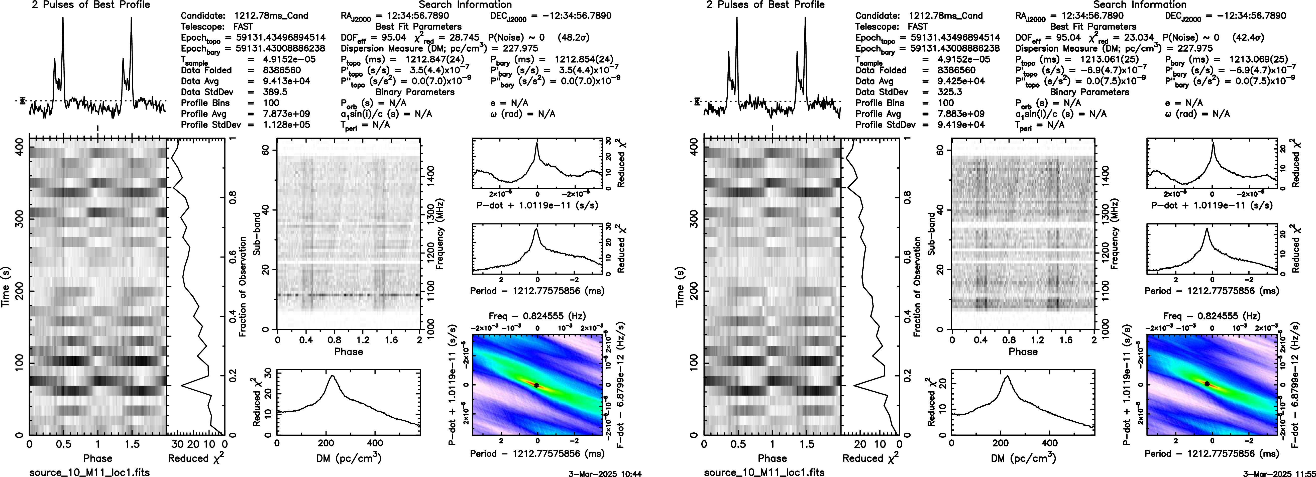
To validate the algorithm’s reliability, we applied the RFI mask generated by mRAID and folded the data with parameters of PSR J1832+0204_P. Figure 6 presents a comparison of folded pulsar data after RFI masking using rfifind (left panel) and mRAID (right panel). Each panel includes key diagnostic plots from the pulsar folding process: the pulse profile (top), time-phase diagram (left lower), frequency-phase diagram (center), dispersion measure (DM) curve, and reduced $\chi^2$
plot. While the pulsar can be clearly detected in both cases, mRAID outperformed rfifind, resulting in a cleaner frequency-phase diagram.
$\chi^2$
plot. While the pulsar can be clearly detected in both cases, mRAID outperformed rfifind, resulting in a cleaner frequency-phase diagram.
4.2. Time domain RFI
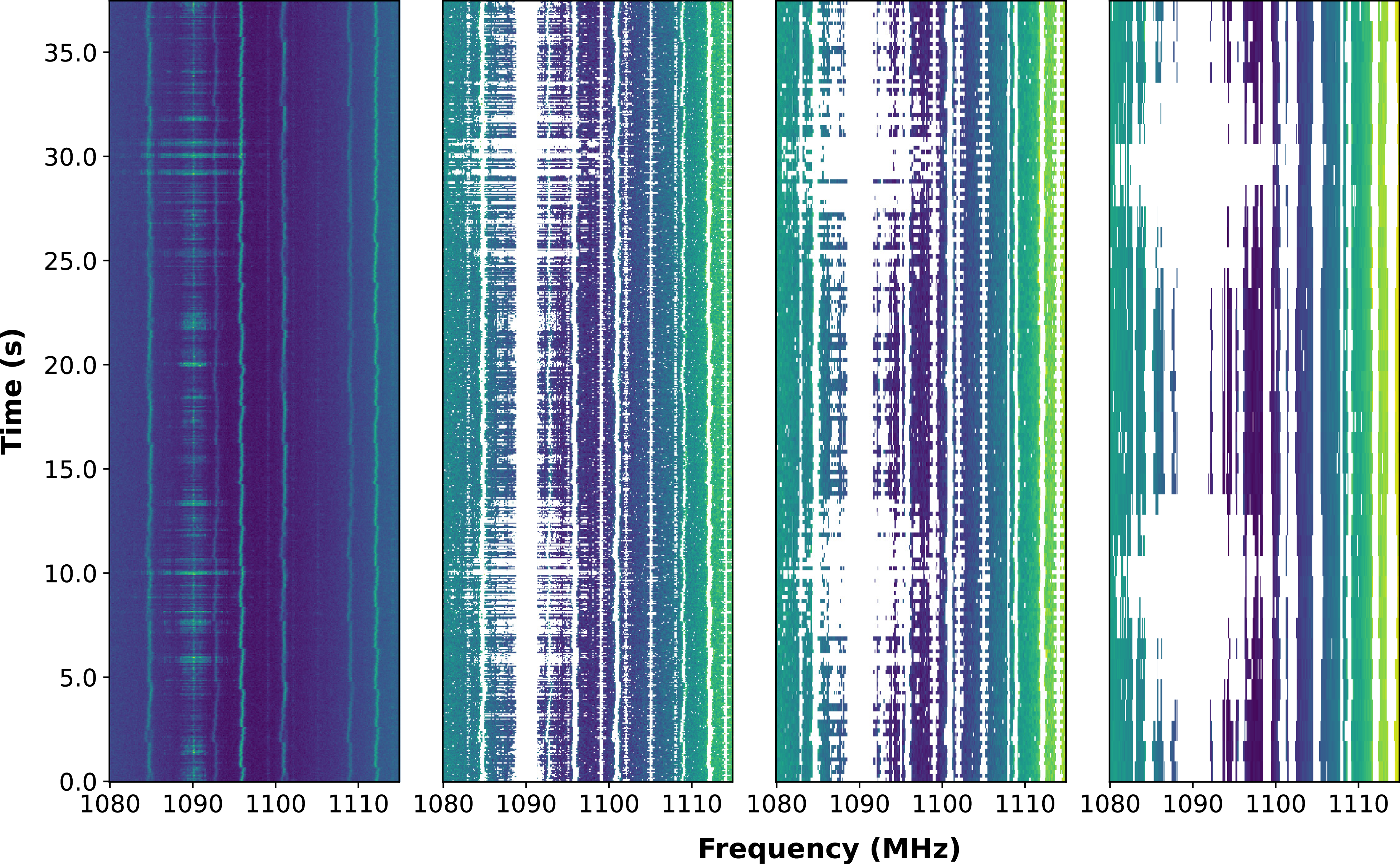
The CCM of multi-beam data offers an efficient approach for identifying RFI on much shorter timescales compared to methods that analyse each beam independently. Figure 7 demonstrates the performance of mRAID in identifying and masking RFI at different time resolutions. The leftmost panel shows the original unmasked dynamic spectrum, while the second to fourth panels display the results after applying mRAID with subinterval lengths of 0.05, 0.20, and 1.00 s, respectively. All panels correspond to the same frequency subband (1 080–1 115 MHz), with time increasing along the vertical axis and frequency along the horizontal axis. At the finest time resolution (0.05 s), transient and narrowband RFI structures are clearly resolved, and mRAID effectively masks these features. As the subinterval time increases, RFI signals are increasingly smeared in time and become more dominant in the averaged spectra. Nonetheless, mRAID maintains robust suppression performance across time scales, successfully identifying both weak and strong RFI features without introducing excessive masking. These results highlight the algorithm’s adaptability to varying temporal resolutions and its advantage over static, threshold-based methods in dynamic RFI environments.
Histogram of dominant eigenvectors of non-RFI channels (those not flagged as RFI in Figure 1) derived for the FAST 19-beam test observations. A Gaussian fit to the distribution is shown as the red line.

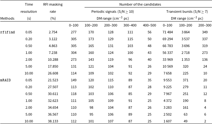
We compare mRAID to rfifind at different time resolutions by applying both to the same data set. Table 1 summarises the RFI masking rates and the number of periodic and transient candidates detected after search. For rfifind, the RFI masking rate gradually increases from 2.754% at 0.05 s to 26.608% at 10.00 s, and the number of periodic and transient candidates across all DM ranges decreases. This outcome is expected, as threshold-based methods are more effective at detecting weak RFI when the integration time is longer. However, for short-duration, transient RFI, these methods tend to be less effective. In contrast, mRAID exhibits a significantly more effective RFI masking rate at all timescales. At 0.05 s, mRAID masks 21.523% of the data, nearly eight times that of rfifind at the same resolution. As the integration time increases to 2.00 s, the masking rate of mRAID reaches 34.654%, compared to 10.288% for rfifind at the same time resolution. This more effective RFI mitigation strategy leads to a smaller number of surviving candidates. For example, at 2.00 s and in the 100–200 cm $^{-3}$
pc DM range, mRAID yields 98 candidates, while rfifind yields 143. Similarly, the number of transient candidates detected, with signal-to-noise ratios (S/N)
$^{-3}$
pc DM range, mRAID yields 98 candidates, while rfifind yields 143. Similarly, the number of transient candidates detected, with signal-to-noise ratios (S/N) $\geq 7$
, is consistently lower for mRAID compared to rfifind across all DM ranges and time resolutions. For instance, at 2.00 s, rfifind detects 33 969 candidates at DM 0–100 cm
$\geq 7$
, is consistently lower for mRAID compared to rfifind across all DM ranges and time resolutions. For instance, at 2.00 s, rfifind detects 33 969 candidates at DM 0–100 cm $^{-3}$
pc, whereas mRAID detects only 3 283. This significant reduction suggests that mRAID suppresses false transient detection more effectively, further improving our sensitivity to weak bursts. Our results indicate that mRAID provides more efficient and effective RFI masking than rfifind, particularly in environments with short-duration (
$^{-3}$
pc, whereas mRAID detects only 3 283. This significant reduction suggests that mRAID suppresses false transient detection more effectively, further improving our sensitivity to weak bursts. Our results indicate that mRAID provides more efficient and effective RFI masking than rfifind, particularly in environments with short-duration ( $ \lt 1.00$
s) interference. With significantly reduced number of candidates, mRAID improves the likelihood of detecting radio bursts by minimising false positives induced by RFI.
$ \lt 1.00$
s) interference. With significantly reduced number of candidates, mRAID improves the likelihood of detecting radio bursts by minimising false positives induced by RFI.
The average percentage of RFI masks for FAST 19 beams data using the rfifind and mRAID methods, as well as the number of the periodic and transient candidates generated using the mask files within different DM ranges.

Time averaged spectrum of each beam of the FAST observation. Raw spectra are shown as black points; results of rfifind are shown as green; results of mRAID are shown as blue. Compared with the raw spectra, while both methods effectively identify strongly RFI-affected channels, mRAID shows superior performance in identifying weak RFI.

4.3. Impacts on astronomical signals
To assess the potential risk of over-flagging genuine astronomical signals, we applied mRAID to data of eleven pulsars observed as part of the FAST pilot pulsar survey at intermediate Galactic latitudes (Zhi et al. Reference Zhi2024). In all cases, mRAID effectively identified and masked RFI-contaminated frequency channels and time intervals while retaining the pulsar signals. Compared with the conventional rfifind method, the integrated S/N of the pulse profiles obtained after RFI masking are comparable (see Table 2). For example, for the bright pulsar J1832+0204_P (Han et al. Reference Han2025), the integrated pulse profile has an S/N of 42 with rfifind and 44 with mRAID, indicating that mRAID does not over-flag the data. For the nulling pulsar J1824 $-$
0127 (Yan et al. Reference Yan2024), with a flux density of
$-$
0127 (Yan et al. Reference Yan2024), with a flux density of $S_{1\,400} = 0.59$
mJy at 1.4 GHz (Lorimer et al. Reference Lorimer2006), we detected 84 single pulses during a 412.00 s observation spanning 165 rotation periods using both mRAID and rfifind. The brightest single pulse reached an S/N of 104, confirming that neither method removed genuine broadband transient signals.
$S_{1\,400} = 0.59$
mJy at 1.4 GHz (Lorimer et al. Reference Lorimer2006), we detected 84 single pulses during a 412.00 s observation spanning 165 rotation periods using both mRAID and rfifind. The brightest single pulse reached an S/N of 104, confirming that neither method removed genuine broadband transient signals.
Comparison of integrated S/N values for pulse profiles generated by the rfifind and mRAID RFI-mitigation techniques.

While mRAID is primarily developed for time domain surveys with high time resolution, it can also be used for continuum or spectral line observations with multi-beam receiver systems. However, our experiments with FAST 19-beam data showed that the neutral hydrogen (HI) line at 1 420 MHz was flagged as RFI by mRAID. This suggests that narrow-band spectral lines detectable across multiple beams, such as HI or maser emissions, can be misidentified as RFI. To address this, we implemented an option in mRAID that allows users to specify frequency ranges to be preserved during the masking process, ensuring that known astronomical spectral lines are retained.
RFI masked data of beam 11 of the FAST observation. Left: results of rfifind; right: results of mRAID. Compared with rfifind, mRAID produces much cleaner data in time and frequency after masking, effectively preserving uncontaminated regions while removing both narrow-band and broadband RFI.

Comparison of the folded pulsar results after RFI masking using the rfifind (left) and mRAID (right). These plots were generated using the prepfold command as part of PRESTO. mRAID performs a more thorough removal of weak narrow-band RFI than rfifind.

RFI masking results of mRAID at different time resolutions. The leftmost panel shows the original dynamic spectrum (unmasked), while the second to fourth panels present the results after applying mRAID with increasing subinterval lengths of 0.05, 0.20 and 1.00 s, respectively. The data correspond to the same frequency subband (1 080–1 115 MHz). These plots demonstrate that mRAID excels at identifying time-domain RFI with sub-second durations and/or periodic patterns.

4.4. Computational performance
We benchmarked the computational performance of mRAID and compared it with that of rfifind using a 20-core CPU cluster running on a Linux operating system. For this evaluation, we used the same FAST data set described in previous sections. Each observation had an integration time of 412.00 s, consisting of 8 388 608 time samples with a sampling interval of 49.152 $\unicode{x03BC}$
s. For a subinterval duration of 1.00 s, we computed a total of 412 CCMs as outlined in Section 3.2, and performed eigenvalue decomposition for each. mRAID completed RFI masking for all 19 beams on a single CPU thread in 12.74 h, while rfifind processed the same data with a 1.00 s integration time in approximately 10.67 h on the same CPU. Thus, even without parallelisation, the computational performance of mRAID is comparable to that of rfifind. Furthermore, because the computation of CCMs and their eigenvalue decompositions are entirely independent across subintervals, the analysis of the FAST data set can, in principle, be parallelised across up to 412 CPUs for this given data set. This approach would greatly accelerate processing and achieve much more efficient RFI masking than rfifind.
$\unicode{x03BC}$
s. For a subinterval duration of 1.00 s, we computed a total of 412 CCMs as outlined in Section 3.2, and performed eigenvalue decomposition for each. mRAID completed RFI masking for all 19 beams on a single CPU thread in 12.74 h, while rfifind processed the same data with a 1.00 s integration time in approximately 10.67 h on the same CPU. Thus, even without parallelisation, the computational performance of mRAID is comparable to that of rfifind. Furthermore, because the computation of CCMs and their eigenvalue decompositions are entirely independent across subintervals, the analysis of the FAST data set can, in principle, be parallelised across up to 412 CPUs for this given data set. This approach would greatly accelerate processing and achieve much more efficient RFI masking than rfifind.
4.5. Key parameters for mRAID
There are a few parameters that are important for RFI masking with mRAID. Here we describe each of them:
-
• Bandpass normalisation parameters: as described in Section 3.1, mRAID employs the ArPLS algorithm for bandpass normalisation. The implementation details and performance of ArPLS have been extensively discussed in previous studies (Zeng et al. Reference Zeng2021; Wang et al. Reference Wang2022). Briefly, the ArPLS algorithm includes three tunable parameters: (1) lam, which controls the smoothness of the estimated baseline – larger values yield smoother backgrounds by imposing stronger penalties on curvature; (2) ratio, which sets the sensitivity of the reweighting scheme to negative deviations – smaller values make the algorithm less tolerant to downward fluctuations; and (3) itermax, which defines the maximum number of iterations for the asymmetric reweighted fitting process – higher values can improve convergence and baseline accuracy at the cost of increased computation time (Baek et al. Reference Baek, Park, Ahn and Choo2015). Depending on the bandpass shape, frequency resolution, and bandwidth of a given observing system, these parameters can be fine-tuned to optimise the bandpass normalisation performance.
-
• Eigenvalue threshold parameter: This parameter sets the threshold for identifying RFI-affected channels. It is defined as an integer multiple of the standard deviation of the eigenvalue distribution, where the standard deviation is automatically estimated by fitting the non-RFI portion of the distribution with a Gaussian model. A smaller value results in more aggressive RFI masking. For the FAST data set used in this work, a threshold of three provided satisfactory performance, while increasing it to five resulted in only about 2% less data being flagged as non-RFI (from about 34.6% to 32.6% averaged across 19 beams).
-
• Eigenvector threshold parameter: This parameter defines the threshold for identifying RFI-affected beams within a given frequency channel. It is expressed as an integer multiple of the standard deviation of the eigenvector distribution. For each beam, the standard deviation is estimated individually by fitting a Gaussian model to the eigenvector elements of non-RFI channels specific to that beam. In our experiments with the FAST dataset, a threshold of one was adopted. This choice is motivated by the high sensitivity of FAST, which causes most RFI sources to be detected across multiple beams, and by the significant overlap between the eigenvector distributions of RFI-affected and clean channels. Varying the eigenvector threshold from one to three resulted in only a minor change in the fraction of masked data – from approximately 34.6% to 31.4% when averaged across the 19 beams, and reduced the number of beams flagged as affected by RFI by one. This indicates that, for the FAST 19-beam dataset, the algorithm’s performance is only weakly sensitive to the specific choice of threshold.
4.6. Limitations
In our current implementation, bandpass normalisation is performed before computing the CCMs and carrying out the eigenvalue decomposition. For the FAST dataset, our results show that mRAID effectively identifies both narrow-band, spiky RFI and broadband RFI. However, broadband and weak RFI may present challenges, as they can mimic bandpass variations and thus be missed by mRAID.
It is also worth noting that, although the current implementation of mRAID supports parallelisation in time, this approach becomes inefficient for short integrations due to the small number of subintervals. A potential improvement would be to enable parallelisation of CCM computation and eigenvalue decomposition across frequency channels, which are fully independent and would allow for more efficient processing.
5. Conclusions
This paper introduces a new RFI identification and masking software package, mRAID, based on the cross-correlation matrix of multi-beam data and eigenvalue decomposition. By constructing the cross-correlation matrix and decomposing it into eigenvalues and eigenvectors, the method identifies and masks RFI in different beams effectively. Compared to traditional threshold-based methods, this approach leverages the inter-beam correlation to tackle RFI under complex conditions.
Experimental results confirm the effectiveness of the proposed approach, particularly in detecting weak RFI signals and operating at short timescales. By leveraging eigenvalue decomposition, the method captures RFI characteristics through the distribution of eigenvalues and eigenvectors, enabling accurate interference identification in different beams. The use of the cross-correlation matrix further enhances robustness against both narrow-band and short-duration RFI. Compared to traditional single-beam thresholding techniques, the proposed method achieves higher detection rates while preserving unaffected data, demonstrating its superior performance in challenging observational environments.
Additionally, the computation of the cross-correlation matrix and eigenvalue decomposition is performed independently for each subinterval and frequency channel. This structure allows for efficient optimisation through parallel processing using CPU multithreading, substantially improving computational efficiency compared to RFI mitigation methods that process each beam individually. The mRAID framework is fully general and can be extended to other multibeam systems, including the PAF installed on Murriyang, the Parkes telescope. Its dependence solely on inter-beam covariance makes it adaptable to different beam layouts and instrumental responses.
Acknowledgement
We would like to thank Simon Johnston, Lister Staveley-Smith and Ron Ekers for useful discussions. This work is supported by the National Natural Science Foundation of China (Nos. 12288102, 12041304, 12273008, 12041303, 12041304, 12403046), the Major Science and Technology Program of Xinjiang Uygur Autonomous Region (No. 2022A03013-3), the National SKA Program of China (Nos. 2022SKA0130100, 2022 SKA0130104, 2020SKA0120200), The research is partly supported by the Operation, Maintenance and Upgrading Fund for Astronomical Telescopes and Facility Instruments, budgeted from the Ministry of Finance of China (MOF) and administrated by the Chinese Academy of Sciences (CAS), the Natural Science and Technology Foundation of Guizhou Province (No. [2023]024), the Guizhou Provincial Basic Research Program (Natural Science) (QiankehejichuMS[2025]266). This work made use of the data from FAST (Five-hundred-meter Aperture Spherical radio Telescope) (https://cstr.cn/31116.02.FAST). FAST is a Chinese national mega-science facility, operated by National Astronomical Observatories, Chinese Academy of Sciences.
Data availability statement
A Python software package of this work is available at https://github.com/juntaobai/mRAID.git.


 Open access