


1. Introduction
Additive manufacturing (AM) enables highly complex geometries and design opportunities that were previously constrained by traditional manufacturing technologies. Metal AM has reached a level of maturity where it is used in production, including relatively high-volume manufacturing, and attracts sustained investment from the automotive and aerospace industries (Reference Delic, Eyers and MikulicDelic et al., 2019; Reference Najmon, Raeisi and TovarNajmon et al., 2019). In contrast, polymer AM is not yet widely adopted in industry because the technology has not demonstrated sufficient reliability. Nevertheless, polymer AM offers several major advantages over metal AM. First, equipment for metal AM is costly, whereas polymers can be processed using low-cost systems. Second, polymer AM is considerably faster; Reference Laban, Mahdi, Samim and CabibihanLaban et al. (2021) reported an 80%-time difference between the two methods, mainly due to the extensive process planning and post-processing required for metal AM. Third, materials for polymer AM are relatively inexpensive, supporting rapid prototyping where functional performance can be explored without a large budget. However, several critical challenges must be addressed before widespread industrial implementation of polymer AM. The fundamental issue is that the process profoundly affects the mechanical properties of manufactured components (Reference Fang, Xiong, Zhou, Tamir, Yan, Wu, Shen and WangFang et al., 2024; Reference Goh, Yap, Tan, Sing, Goh and YeongGoh et al., 2020; Reference Letcher and WaytashekLetcher & Waytashek, 2015), leaving load-bearing capabilities uncertain. Consequently, recent literature argues that process documentation and control are the main barrier that must be overcome to enable polymer AM (Reference Fang, Xiong, Zhou, Tamir, Yan, Wu, Shen and WangFang et al., 2024; Reference Isiani, Crittenden, Weiss, Odirachukwu, Jha, Johnson and AbikaIsiani et al., 2025).
In polymer AM, the most used technologies include Powder Bed Fusion (PBF), VAT photopolymerization, and Material Extrusion (MEX). PBF has already been introduced for end-use manufacturing because it produces parts with near-isotropic properties. In the research literature, polymers are classified as consumer-grade polymers and high-performance polymers (Reference Das, Chatham, Fallon, Zawaski, Gilmer, Williams and BortnerDas et al., 2020). However, PBF is relatively slow, similar to metal PBF, and the material options are limited to materials such as Polyamide, having the highest strength available, with a reported UTS of 53 MPa (Reference Olejarczyk, Gruber, Gazińska, Krokos, Ziółkowski, Szymczyk-Ziółkowska, Grochowska and KurzynowskiOlejarczyk et al., 2024). VAT photopolymerization differs in printing speed; it has become one of the fastest AM methods, reaching 1000 mm/h (Reference Paral, Lin, Cheng, Lin and JengParal et al., 2023). Because the process relies on UV light to solidify liquid resin, it is restricted to UV-curable materials. Available VAT polymers include NH-09, poly (ethylene glycol) diacrylate (PEGDA), and 1,6-hexanediol diacrylate (HDDA), with a maximum reported strength of 39.9 MPa (Reference Liu, Yang, Sun, Yang and LiLiu et al., 2019), although continuous-fibre VAT has reached a UTS of 286.6 MPa (Reference Lu, Han, Gleadall, Chen, Zhu and ZhaoLu et al., 2022). In MEX, many of the material limitations observed in PBF and VAT are addressed. Higher processing temperatures and heated chambers allow the use of a wide range of polymers, enabling low-cost prototyping and subsequent fabrication in high-performance materials once designs are finalized. MEX also offers substantial scaling potential, exemplified by Big Area Additive Manufacturing (BAAM) (Reference Chesser, Post, Roschli, Carnal, Lind, Borish and LoveChesser et al., 2019; Reference Duty, Kunc, Compton, Post, Erdman, Smith, Lind, Lloyd and LoveDuty et al., 2017). Furthermore, MEX can deliver mechanical properties not attainable with other polymer AM technologies. Current literature describes MEX materials in a pyramid classification, where processability decreases toward the apex. At the top of this pyramid, Poly Ether Ether Ketone (PEEK) currently dominates the high-performance market.
The PEEK polymer with the highest reported performance is TECAFIL PEEK VX CF30, with XZ ≈ 199 MPa and ZX ≈ 62 MPa according to the manufacturer’s datasheet (Germany, Nufringen, Ensinger). With improved temperature control, new printer manufacturers such as Orion AM have reported strengths up to 100 MPa by trial-and-error calibration and visual evaluation during manufacturing (Reference OrionOrion AM, 2025). However, their hardware still lacks integrated process monitoring and control. Given the scalability of MEX, its short manufacturing times, relatively low hardware and material costs, and its potential for high mechanical performance, developing robust process monitoring and control for this technology is the most logical path forward.
Literature has shown that processing temperature has a major effect on mechanical properties (Reference Amlie, Fylling, Eikevåg, Nesheim, Steinert and ElverumAmlie et al., 2023; Reference Bjørken, Andresen, Eikevåg, Steinert and ElverumBjørken et al., 2022). The critical temperature to monitor is the temperature of the preceding layer immediately before deposition, denoted Lp-1 in (Reference Seppala and MiglerSeppala & Migler, 2016). In this article we have chosen to refer to this temperature as Pre-Deposition layer Temperature (PDT) to specify that the temperature of the layer (Lp-1) is measured immediately before deposition. PDT can be measured using infrared pyrometers (Reference Amlie, Fylling, Eikevåg, Nesheim, Steinert and ElverumAmlie et al., 2023) or infrared thermography (IRT) (Reference Dupas, Elverum, Sasson and EikevågDupas et al., 2026). While pyrometers measure a single point, an IR camera captures temperature pixel by pixel, limited only by the camera’s resolution. Using IRT, several studies have successfully captured both thermal history and processing temperatures during MEX (Reference Nesheim, Eikevåg, Steinert and ElverumNesheim et al., 2025; Reference SadafSadaf, 2024; Reference Seppala and MiglerSeppala & Migler, 2016).
In-situ temperature monitoring can support process control because the PDT can be used in a closed-loop system (Reference Dupas, Elverum, Sasson and EikevågDupas et al., 2026). This approach can improve part performance and provides an initial means of documenting the thermal history for certification. Other studies have attempted to link thermal to spatial measurements to obtain a deeper understanding of the printed component (Reference Amlie, Fylling, Eikevåg, Nesheim, Steinert and ElverumAmlie et al., 2023). However, this proved challenging because the G-code required extensive manual editing, greatly increasing data volume, and because the study used a pyrometer capable of measuring temperature in only one print direction. An alternative to extracting coordinates from G-code—which provides positions only at direction changes and leaves large gaps—is to use electronics common in CNC equipment since the 1980s. Encoders have been shown to accurately capture the movement of the toolhead (Reference Herrojo, Paredes and MartínHerrojo et al., 2020).
This paper explores the concept of thermal clouds, in which temperatures captured by IRT are synchronized with coordinates provided by encoders. The approach was developed on a low-cost machine using Polylactic Acid (PLA) to accelerate prototyping while remaining applicable to any MEX system. The objective is to monitor the complete thermal history and ensure that thermal values are traceable to the printed geometry. Each thermal node in the resulting mesh can be linked to mechanical properties (Reference Bjørken, Andresen, Eikevåg, Steinert and ElverumBjørken et al., 2022; Reference Ørnes, Elverum, Sasson and EikevågØrnes et al., 2026). To evaluate the concept, the encoders were validated experimentally. Vectors computed from the encoders were used to identify the correct IR pixel for each measurement. Limitations were then identified, and filtering was introduced to address fraudulent data observed in three geometries—complex, advanced, and simple. All components were filtered, excluding temperatures that were either too high or too low and where the extruder was traveling, not extruding. This approach represents a first step toward process certification by capturing sufficient data to support simulations of MEX-printed components.
2. Method
A thermal cloud of a 3D-printed part is a temperature mesh in which each node has its corresponding spatial value that can potentially be linked to mechanical properties. Creating such a thermal cloud requires several prerequisites, ranging from part design and slicing to data gathering and synchronization. The ultimate goal of part certification is supported by a broader understanding of the spatio–thermal properties of the printed part and, more specifically, by relating local temperature measurements to material strength (Reference Bjørken, Andresen, Eikevåg, Steinert and ElverumBjørken et al., 2022). Figure 1 presents our framework for part certification by MEX, where yellow denotes the traditional process, light beige the added sensors used to capture spatial and thermal data and purple the data-processing steps leading toward certification.
Thermal certification workflow

2.1. Hardware
The Prusa XL (Czech Republic, Prague, Prusa Research) with two extruder heads was chosen because of its easy access to the stepper motors, low cost, and CoreXY architecture which allows for rapid prototyping. The CoreXY system uses two XY stepper motors (Figure 2.1Bx, 2.1By) and two Z-axis stepper motors (Figure 2.1Bz). Only one Z-axis motor needed to be monitored because the two motors operate symmetrically. During in-plane diagonal movement, only one XY stepper motor rotates, whereas both motors rotate during all other in-plane movements. To capture the toolhead movement and the part height, encoders were added (Figure 2.1c).
For 3D printing, the thermal camera must offer high accuracy and precision to resolve small temperature differences. The TC001 Plus (USA, Rockaway, TOPDON) (Figure 2.1D) is a 256×192-pixel IR camera with a 25 Hz refresh rate. It measures temperatures from −20 °C to 550 °C with an accuracy of 2 °C and a resolution of 0.1 °C. The camera was installed in a 3D-printed holder mounted to the side of the printer with three screws so that it follows the printhead movement (Figure 2.2). This mounting design provides a clear line of sight to the nozzle and reduces vibration through a reinforced support structure for the camera arm.
1: Hardware setup and informational flow; 2: Camera setup

The camera was mounted 113.8 mm from the nozzle at a 21.3° angle (Figure 2.2), providing a horizontal field of view (FOV) of approximately 124 mm and a vertical FOV of 73 mm. This results in an instantaneous FOV horizontally and vertically of 0.646 mm/pixel and 0.285 mm/pixel respectively. The camera transfers raw data through a USB-C connector.
The experiment used an AMS AS5600 OSRAM encoder chip with a 12-bit resolution (Austria, Premstätten, ams-OSRAM AG), giving a theoretical accuracy of 0.087°. The manufacturer specifies an accuracy of 0.4°, whereas practical raw angle data can vary by up to 2° (Lingib, 2025). The difference between theoretical and practical performance is attributed to off-centre magnet alignment, chip–magnet spacing outside the 0.5–3 mm range, and magnetic-field distortion. Calibration is therefore required to accurately capture toolhead movement. The encoders were mounted on the X and Y motors and on one of the Z motors. The X and Y encoder chips were positioned 2.65 mm from the magnet, and the Z encoder chip at 2.72 mm. The diametric magnet was mounted on the stepper-motor axle using a laser-cut centring piece to ensure accurate placement. The encoders share the same I2C address, so a multiplexer was required to assign each encoder a distinct address. An Adafruit TCA9546A I²C multiplexer (USA, New York, Adafruit Industries) was used for this purpose. The multiplexer and encoders were connected through a breakout board to an Arduino Uno (Italy, Monza, Arduino AG), which logged the data to the PC (Figure 2.1). The sampling interval was set to 13.3 ms, corresponding to a sampling rate of approximately 75 Hz to avoid aliasing.
2.2. Printing and manufacturing
To gather data from both the encoders and the IR camera, a dedicated printing procedure was developed. First, the IR camera was powered on at ambient temperature. The G-code file was then started with a custom startup and end G-code. To ensure correct encoder initialization, the startup routine homed the extruder head and waited in this position for 40 s. After initialization, both the camera and encoders were set to record. When the print was completed, recording from both systems was stopped, and each dataset was saved to an individual CSV file. All components were printed using Prusament PLA Jet Black (Czech Republic, Prague, Prusa Research). The printer settings were: 50% infill, fan off to not disturb heat distribution and increase thermal differences based on geometry, 0.25-mm layer height, 225 °C extruder temperature, 60 °C bed temperature, and a 0.4-mm nozzle. PLA has an emissivity of approximately 0.95 (Reference Gholami, Lawan, Luengrojanakul, Ebrahimi, Ahn and RimdusitGholami et al., 2024).
2.3. Design of experiment (exploring the thermal clouds reliability and accuracy)
The first step toward part certification is the implementation of sensors for additional process monitoring, and the added sensors must be validated for accuracy to ensure proper product documentation. The encoders measure the rotation of the stepper-motor axle, which does not directly provide the extruder position. To obtain accurate positions, the encoder outputs must be multiplied by constants Rc and P, derived from measurements of the belt connector for X and Y or the lead screw for Z, respectively. An accuracy test was performed to verify these constants. Because the Prusa XL uses a CoreXY system—where both X and Y stepper motors rotate during in-plane movement—the same constant Rc was used for both axes. The constant P for the Z stepper motors were assumed to be identical. Reference Amlie, Fylling, Eikevåg, Nesheim, Steinert and ElverumAmlie et al. (2023) reported Rc = 12.73 and P = 8.0 for a CoreXY system, but differences in encoder implementation and motor characteristics required system-specific calibration. Therefore, an accuracy test was designed to compare encoder-derived spatial measurements with the positions logged by the Prusa XL. The test also compared different candidate constants to identify optimal values, Ro and Po. For this purpose, the printer was moved 50 mm in X and 30 mm in Z, and the resulting encoder data were divided by the printer-reported movements and multiplied by the initial Rc and P values. These updated constants were used in Test C (Figure 2). Test A values were chosen lower than those in Test B for comparison.
Rc and P for encoder calibration experiment

The calibration test for XY was conducted with constructing a mesh of points in the plane. First, measuring X between 0 mm and 350 mm with increments of 50 mm. The Y value was increased from 0 mm to 300 mm in 100 mm increments. Each node in the generated mesh was first measured for the X values, thereafter, repeating the whole process, only now switching the variables, measuring Y. In the Z direction the encoder and printer values were measured every 30 mm. The goal of the test is to observe which encoder errors are closest to 0. Reference Turek, Bielarski, Czapla, Futoma, Hajder, Misiura, Turek, Bielarski, Czapla, Futoma, Hajder and MisiuraTurek et al. (2025) recommends a tolerance of ±0.2 mm for MEX additive manufacturing errors. Consequently, an error of ±0.2 mm is an acceptable result for the encoder calibration.
2.4. Data-loss in thermal monitoring
Material bonding strength is a critical characteristic for load bearing application of a MEX-manufactured parts (Reference Liaw, Tolbert, Chow and GuvendirenLiaw et al., 2021). Calculating bonding strength requires the PDT (Reference Seppala and MiglerSeppala & Migler, 2016). Accordingly, the temperature was measured from the blue pixels in the half circle surrounding the nozzle (Figure 3). The radius of this half circle is referred to as R. Using encoder data, the positional change between time steps was determined and translated into a travel angle. The pixel on the half circle with the corresponding travel angle was selected, and its temperature was recorded, correlating to PDT. Each data row therefore contains the nozzle position and the associated PDT. A key challenge is selecting a radius small enough to capture PDT accurately during small extruder movements while avoiding thermal noise from the nozzle. A smaller R increases sensitivity to vibration, causing the half-circle pixels to shift toward the nozzle—raising the measured temperature—or away from the intended point, capturing background values. In this study, three components were investigated: a Cubesat (complex geometry), a Benchy (advanced geometry), and a dogbone (simple geometry). All components were printed using radii of 5 pixels (R5) and 10 pixels (R10), as shown in Figures 3a and 3b. The Benchys and dogbones were oriented with their longest uniaxial dimension perpendicular to the camera (Figure 3) to maximize the number of usable pixels.
IR camera view; half circle (blue for illustration purposes) with centre in the red point fixated on the nozzle; Figure 3a has a radius of 5 pixels(R5) whilst 3b has a radius of 10 pixels(R10)

The goal is to retain as many nodes as possible while maintaining accuracy, therefore, different geometries were manufactured. The Cubesat (Figure 4.2) contains small struts that generate frequent travel moves and are expected to cause significant data loss. In contrast, the dogbone (Figure 4.1) has a continuous geometry and is expected to exhibit comparatively low loss. For the Benchy (Figure 4.3), data loss is anticipated due to the frequent geometric transitions throughout the build. We analyse the node loss produced by each filter to determine the conditions that yield accurate thermal-cloud measurements.
Test geometries: (4.1) dogbone is divided into three parts and temperatures are observed at points t; rectangle (4.1a) t1 and t2, line (4.1b) t3 and circle (4.1c) t4 and t5; (4.2) Cubesat and (4.3) Benchy

2.5. Data synchronization and filtering
Data from the IR camera were gathered using the Python library OpenCV together with the time and csv modules. To log encoder data from the Arduino IDE via Python, the PySerial and pandas libraries were used, along with the serial and threading modules. This enabled the use of the time.time() function, which provides Unix timestamps, unlike the relative timekeeping in the Arduino IDE. Because the thermal camera records absolute timestamps, both datasets could be aligned through their shared Unix time factor. Using this common reference, the datasets were merged with pandas’ merge_asof function using the nearest parameter, matching each encoder entry to the closest camera timestamp Before merging, the encoder dataset was filtered by removing positional data outside the manually defined build volume. The two datasets were then trimmed to the length of the smaller one, and encoder timestamps without a corresponding thermal-camera match were dropped. Datapoints with PDT values above 130 °C or below 40 °C were excluded because such temperatures are not representative of PLA. The maximum extruder velocity occurs during travel moves at 400 mm/s, followed by solid infill at 140 mm/s. Given the encoder sampling interval, these correspond to 5.332 mm/interval and 1.866 mm/interval, respectively. By computing the norm of the change in X and Y and filtering out values above 1.9 mm/interval, datapoints associated with travel moves were removed. After filtering, the remaining datapoints were plotted using the pydeck library.
2.6. Thermal effect of geometry
To know the effects of geometrical variation a custom made dogbone was designed to test thermal geometry-based deviations. The circular section (Figure 4.1c) is expected to have a high centre temperature whilst the edge temperature will be lower. For the long and thin middle section (Figure 4.1b), the thermal density is lower and correspondingly lower temperatures are anticipated compared to the other geometries. In Figure 4.1a the temperatures are expected to resemble the ones in the circular part, however the corners should be cooler due to more surface area exposed to the surroundings.
3. Results
3.1. Encoders
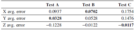
Judging by the requirements presented by Reference Turek, Bielarski, Czapla, Futoma, Hajder, Misiura, Turek, Bielarski, Czapla, Futoma, Hajder and MisiuraTurek et al. (2025) all avg. errors for each test comply with the given tolerance of ±0.2 mm as can be observed in Table 1. However, some individual errors for test A and test C surpass the allowed tolerance for Z axis and XY axis respectively (Figure 5).
Average encoder data results

For the XY axes test A and B are superior, nearing the red error equals zero line drawn into the plots in Figure 5. Test A preforms remarkably worse than the other tests for the Z axis. This shows that test B, with original values of Rc = 12.73 and P = 8.0 has the best fit of the three. However, for the XY axes test A is as practically as good as test B. This simple experiment verifies that an optimal Ro is found in the range 12.729 < Ro < 12.7369, whilst an optimal value, Po, will be found in the range Po ≥ 8.0.
Plot of Encoder test results sorted per axis; X-axis(a), Y-axis(b) and Z-axis(c)

3.2. Thermal effect of geometry
Evaluating the thermal effect on the dogbone’s geometry, t1, t3 and t4 are observed lower than t2 and t5 that are located on the edge of the printed part (Table 2). Moreover, t3 is lower than both t1 and t4, although t3 is not lower than t1 for R10.
PDT (in °C) extracted from dogbone, R5 and R10

Figure 6 shows a higher concentration of red nodes in the rectangular and circular regions than in the middle section. The effect of radius is also evident: the temperatures in the upper part of the circle are lower in Figure 6b than in Figure 6a, demonstrating the influence of the chosen radius on the measured PDT.
Dogbone sliced in the middle; R5(a) and R10(b)

3.3. Part certification
The effect of the filtering process can be seen in Table 3:
Filtering data loss and resulting average temperatures for R5 and R10

Figure 7 presents the thermal clouds of the different geometries after filtering. By comparing the post-merged and post-filtered datasets, the variations between objects and radii become apparent. For the dogbones, the minimum- and maximum temperature, and travel filters removed 9.01% of nodes for R5 and 5.63% for R10. Owing to the simplicity and density of the geometry, neither dogbone had nodes excluded by the minimum filter, and the maximum filter removed more nodes for R5 than for R10 (7.96% vs. 4.56%). The Cubesat consists of many thin struts and walls, causing the camera to capture background values and nodes from neighbouring layers. Filtering excluded 10.08% (R5) and 20.68% (R10), with the minimum filter responsible for 6.07% and 17.84%, respectively. This difference is evident in Figure 7e, where several struts show missing nodes, whereas Figure 7b shows fewer losses. Moreover, the Benchy also shows a substantial difference between R5 and R10, particularly seen on the hull of Figure 7c and Figure 7f. The Benchy R5 was filtered 12.01% whilst R10 was filtered 10.02%. For all objects the average temperature was higher for R5 than R10.
Overview over 3D printed parts and corresponding thermal clouds; (a) Dogbone R5, (b) Cubesat R5, (c) Benchy R5. (d) Dogbone R10, (e) Cubesat R10 and (f) Benchy R10

Thermal and geometric effects of capturing data is showcased in Figure 8. The frontside of the Benchy (Figure 8b, e) is the side closest to the camera whilst the backside (Figure 8a, d) is the side furthest away from the camera.
Comparison of Benchy frontside, backside and backend; backside: R5(a) and R10(d); frontside: R5(b) and R10(e); backend: R5(c) and R10(f)

Figure 8 Long description
Panel A: A heat map showing the temperature distribution in a 3D-printed object with a temperature range from 40 to 130 degrees Celsius. The object is depicted from the front side with a resolution of R5. Panel B: A heat map showing the temperature distribution in a 3D-printed object with a temperature range from 40 to 130 degrees Celsius. The object is depicted from the back side with a resolution of R5. Panel C: A zoomed-in view of the heat map from Panel B, highlighting specific areas of temperature distribution. Panel D: A heat map showing the temperature distribution in a 3D-printed object with a temperature range from 40 to 130 degrees Celsius. The object is depicted from the front side with a resolution of R10. Panel E: A heat map showing the temperature distribution in a 3D-printed object with a temperature range from 40 to 130 degrees Celsius. The object is depicted from the back side with a resolution of R10. Panel F: A zoomed-in view of the heat map from Panel E, highlighting specific areas of temperature distribution.
As previously mentioned, the PDTs for R10 (Figure 8, row 2) are lower than R5 (Figure 8, row 1), this is very clearly seen in Figure 8. The box on the backend (Figure 8c, f) was poorly captured due to the camera not capturing nodes while going directly away from the camera.
4. Discussion
In this study, encoders and an IR camera were used to obtain spatio-thermal data. The spatial data from the encoders were evaluated through a calibration test, but further testing is needed to improve accuracy and quantify precision. Future calibration should include more measurements within the optimal range and repeated trials. After trimming, merging, and filtering, the spatial and thermal datasets provided a more realistic representation of the printed parts Two radii, R5 and R10, were tested for PDT extraction. All three components exhibited higher temperatures for R5 than for R10, with the largest difference observed in the Cubesat (6.53 °C). This is likely because R10 more frequently measured background values, while R5 may have captured thermal noise from the nozzle or a recently deposited layer. As noted by Reference Dupas, Elverum, Sasson and EikevågDupas et al. (2026), identifying an optimal radius is an important area for future work. In the Cubesat, R10 did not capture thin struts sufficiently: the minimum-temperature filter removed 17.84% of nodes for R10, compared with 6.07% for R5. In the dogbone the minimum filter was not activated, due to the higher temperature encountered printing a solid component, as expected. The dogbone also demonstrated clear temperature differences across its geometry, driven by variation in thermal conduction within the PLA relative to the surrounding air at the edges.
Future research should have at least two, preferably four, cameras to capture all in-plane directions. The frontside of the Benchy is notably colder than the backside, because of limited camera coverage. This limitation reduces the number of usable datapoints by approximately 50%, the filtering approach also requires improvement. Ideally, expected temperature ranges should be estimated for each cross-sectional area and layer so that a variable temperature filter can be applied, allowing unrealistic values to be removed more effectively than with the current fixed thresholds. Additionally, an edge-detection filter, as described by Kuriachen et al. (2025), should be implemented to further improve measurement accuracy.
An important question for future work is how reliable 25 Hz thermal cameras are when printers operate at top speeds of 400 mm/s with accelerations of 5,000 mm/s², especially as new systems already reach 600 mm/s and 30,000 mm/s² (Creality K2 Plus, China, Shenzhen, Creality). Determining the sampling frequency required for IR cameras relative to printer motion profiles is therefore essential. In addition, a full calibration of emissivity, offset, and scaling should be performed for the IR camera.
Once these issues are addressed, strength prediction based on thermal analysis becomes feasible. With accurate and reliable data, the correlation between UTS and temperature presented by Reference Bjørken, Andresen, Eikevåg, Steinert and ElverumBjørken et al. (2022) can be used to estimate component strength, predict local variations, or even assess individual nodes. Such predictive capability will be crucial for manufacturing high-performance polymers (HPP) for strength-critical applications. Monitoring HPP manufacturing will require placing stepper motors and thermal cameras outside the heated zone due to the high processing temperatures. To support future IRT applications for HPP, a reliable and accurate data-generation system for thermal-cloud analysis is needed. This article provides the initial steps in thermal cloud analysis for strength prediction and discusses what areas need to be studied to achieve a satisfactory result.
5. Conclusion
In this study a system for capturing in-situ thermal data in MEX was developed, where IRT was integrated with encoder-based spatial tracking to create thermal clouds. The proposed system enables synchronisation of temperature and positional data, providing a foundation for strength prediction and part certification in MEX. Experimental results show that positional accuracy of ±0.2 mm is achievable with encoder calibration. Analysis of thermal clouds for different geometries found that thermal distribution is influenced by measurement radius and part shape. Smaller radius (R5) measure higher average temperatures but also introduce potential thermal noise. Unrealistic data points were removed with filtering strategies, though future work should implement adaptive filters and edge detection to improve reliability and precision. Furthermore, a single-camera coverage and limited sample rates highlight the need for multi-camera setups together with high-frequency sensors to accommodate high-speed printing.
Acknowledgement
Thank you to Vegar Stubberud and Erik Amlie for help with encoders and getting started. Thank you to Martin Steinert for letting me occupy TrollLabs with my printer for 2 months.











 Open access

